Deep-Learning-Based Hydrostatic Curve Modeling for Stability Calculation of Chine-Type Small Ships

Capsizing accidents are regarded as marine accidents with a high rate of casualties per accident. Approximately 89% of all such accidents occur in small ships (vessels with gross tonnage less than 10 tons). Stability calculations are critical for assessing the risk of capsizing incidents and evaluating a ship's seaworthiness. Despite the high frequency of capsizing accidents involving small ships, they are generally exempt from adhering to stability regulations, thus remaining systemically exposed to the risk of capsizing. Moreover, the absence of essential design documents complicates direct ship stability calculations. This study utilizes hull form feature data—obtained from the general arrangement of small ships—as input for a deep learning model. The model is structured as a multilayer neural network and aims to infer hydrostatic curves, which is required data for stability calculations.

Keywords:

Subject: Engineering - Marine Engineering

1. Introduction

1.1. Background of Research

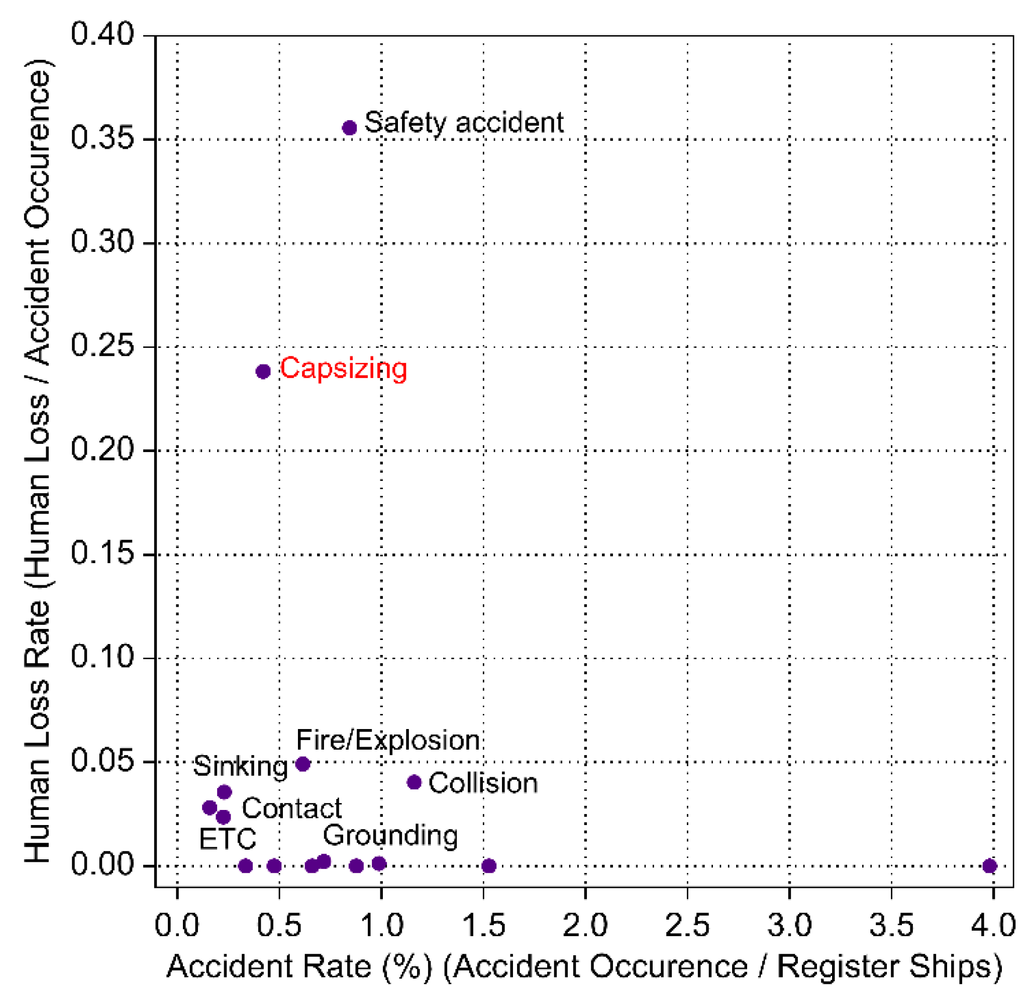
Capsizing accidents occur when external forces cause a stable ship to lose its stability, leading to overturning. Since 2018, an average of 92 such incidents have occurred annually. As show in Figure 1, the rate of human casualties (number of deaths and missing persons per incident) per capsizing incident is 0.238 (casualties/incident), making it the second-highest type of marine accident in terms of human casualties, following safety incidents (0.355 casualties/incident). Over the past five years since 2018, there have been 109 deaths and missing persons. During the same period, 480 ships were involved in capsizing incidents, of which small ships accounted for 89% (428 ships). These statistics confirm that capsizing is a high-risk maritime accident, particularly dangerous to human life on small ships, as found in the survey.

Despite their relatively high frequency of capsizing accidents, small ships are exempt from regulations closely related to their seaworthiness evaluation, specifically in terms of stability standards. Small ships that are not subject to stability regulations lack even minimal assessments of seaworthiness. Essential design documents required for stability calculations—such as general arrangement, lines, midship section, and construction profile and deck plan—are often missing. This makes direct calculations of stability practically difficult. Therefore, there is a pressing need to assess whether appropriate seaworthiness can be ensured through stability calculations, as small ships are systematically exposed to the risk of capsizing. As the majority of domestic coastal ships are chine-type fiberglass reinforced plastic (FRP) vessels, we use key hull form feature data available from limited design documents, such as the general arrangement, as input. As show in Figure 2, we apply a multilayer neural network-based deep learning model to infer hydrostatic curves. This is to evaluate the possibility of direct stability calculations for small ships.

1.2. Status of Related Research

Research on the hull form features of small ships primarily focuses on improving resistance and stability [1,2,3]. In particular, most studies on stability performance have focused on small fishing vessels, considering that the majority of small ships are fishing boats. These studies often involve the development of simplified formulas for estimating GM (metacentric height) due to the exemption of stability tests for fishing vessels under 24 meters in length, or they perform estimates based on stability standards for ships with a length of 24 meters or more [4,5]. Some countries have partially adopted these stability standards for small ships; however, such adoption has often been found to be impractical due to differences in basic hull shapes and the distribution of key dimensions [6]. Studies on the chine shape of small ships primarily aim to improve resistance performance in high-speed hulls [7]. Although some research has been conducted on stability estimation for small ships and the application of stability standards for larger vessels (24 meters in length or larger) [8], systematic studies on the change in stability performance due to chine distribution have been relatively neglected.

Research on artificial intelligence (AI) in shipbuilding and the maritime industry has mostly focused on improving production efficiency through image processing, hull development, and the estimation of preliminary design data. Some studies on large ships include the estimation of optimal stern shapes using a convolutional neural network (CNN) [9], the development of learning systems for the classification and bending information of shell plates [10], and studies on preliminary light weight estimates using deep neural networks (DNN) [11]. Previous studies using AI techniques related to small ships include the use of DNN for estimating key dimensions of small ships [12] and the development of real-time distress recognition systems using real-time video from small ships [13]. However, no studies have investigated the hull form features and stability related to small ships.

2. Ship Stability and Hydrostatic Curve

2.1. Ship Stability Calculation

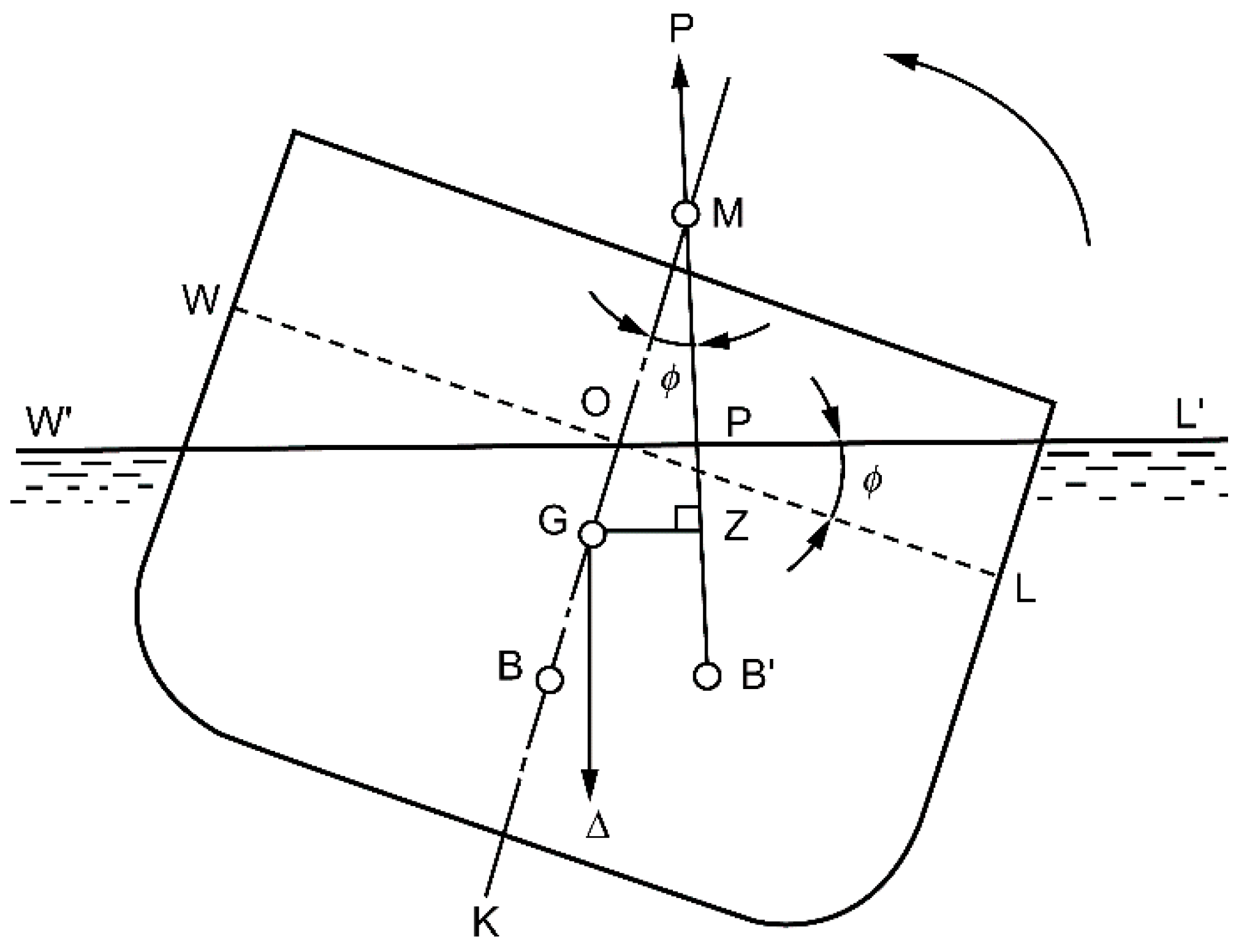
The stability of a ship refers to the force that enables the ship to return to its original equilibrium state when inclined by an external force. Stability depends on factors such as the ship’s center of gravity, displacement, and area moment of inertia with respect to the water plane shape, serving as a minimum criterion for assessing the ship’s seaworthiness.

Initial stability corresponds to the restoring moment at a small transverse inclination angle (

φ

), as depicted in Figure 3.

Stability (restoring moment) = W × \bar{G Z} = W × \bar{G M} × s i n φ,

where \bar{G M} = \bar{K M} - \bar{K G} = \bar{K B} - \bar{B M} - \bar{K G} = \bar{K B} + \frac{I_{t}}{\nabla} - \bar{K G}

Here, W is the displacement, ▽ is the displaced volume, M is the position of transverse metacenter, B is the center of buoyancy, G is the center of gravity, and I_t is the transverse moment of inertia.

Stability is calculated using the ship’s center of gravity (G) obtained through incline tests and the hydrostatic curve. For chine-type vessels, the ship’s water plane shape and the transverse moment of inertia (It) are determined by the arrangement of the chines. This affects the position of the metacenter in initial stability calculations. Because these values can significantly change depending on the chine shape, it can be assumed that the stability characteristics of small ships are determined by the shape and arrangement of the chines.

2.2. Hydrostatic Curve

The hydrostatic curve calculates changes in displacement with respect to changes in the draft of the ship. It represents the distribution of corresponding hydrostatic characteristics of the ship, either graphically or in tabular form. These characteristics include various coefficients such as draft-specific displacement, center of buoyancy (LCB, KB), water plane area (A_w), and wetted surface area, as well as the block coefficient (C_B). These data are essential for calculating ship stability. Lines indicating the accurate hull shape schematics below the waterline are crucial for creating the hydrostatic curve. Many small ships are often exempt from having these design documents (Lines), making direct stability calculations challenging.

3. Deep Learning Data Configuration

The training data consist of 430 ships for which hydrostatic data could be calculated, limited to ships propelled by conventional propulsion systems such as internal combustion engines and propellers. The hydrostatic data calculations include only the main hull and the box keel, excluding additional structures such as the side appendage and stern wedge.

3.1. Dimensionless Learning Data

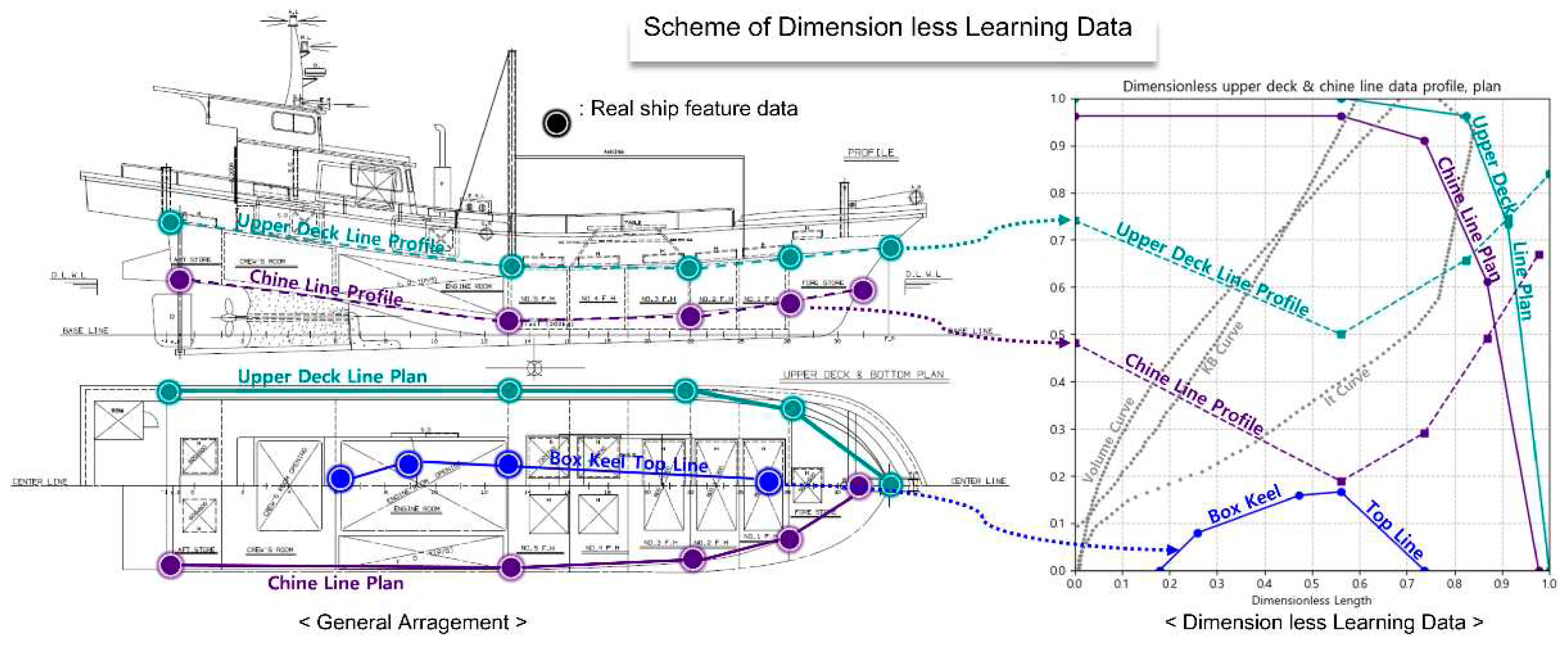
The input data for deep learning, referred to as feature data, consists of key hull form features. These include principal dimension ratios, upper deck data, and details on the chine and box keel, all of which can be obtained from a general arrangement drawing.

To enhance the effectiveness of deep learning training and facilitate intuitive comparisons and parameter utilization, we have converted the training data to be dimensionless. The offset coordinates in length, width, and depth dimensions are normalized to dimensionless values between 0 and 1, based on the aft end, centerline, and baseline of the ship, respectively. Individual elements of hydrostatic data, such as area, volume, and moment of inertia, were made dimensionless by converting them into ratios corresponding to specific ship features (refer to Table 1).

As shown in Figure 4, various linear characteristics of the training data can be plotted on the same [0, 1] plane. This allows for easy comparison between different datasets and an intuitive understanding of the correlations among them by overlaying other dimensionless data (hydrostatic curve).

3.2. Deep Learning Range

To investigate the operational conditions of small ships, we examined draft and displacement across various loading conditions, including light ship and full load conditions (refer to Table 2).

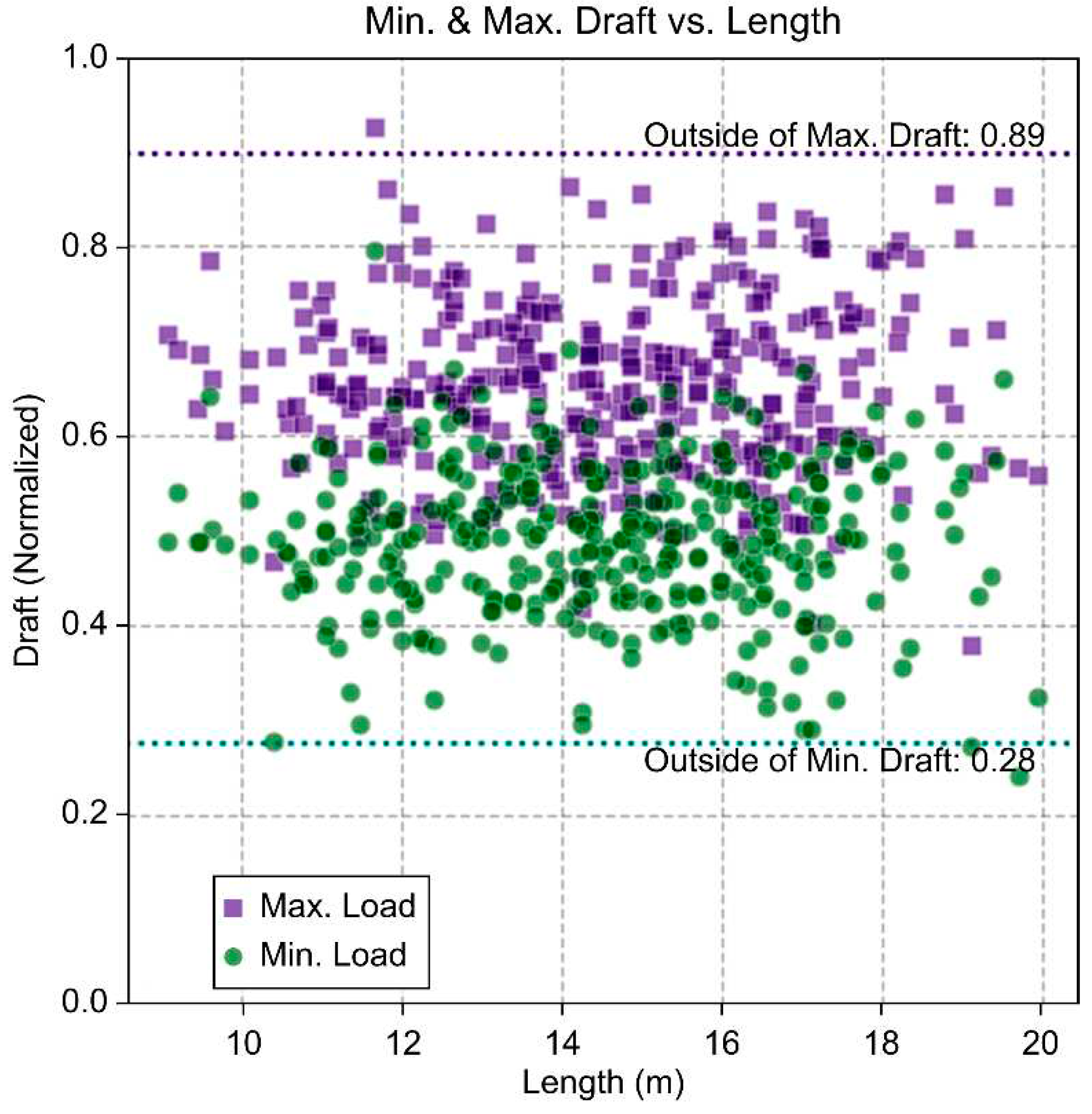
The actual operational draft range for small ships can be assumed to span from light ship to full load conditions. As shown in Figure 5, by applying a method that identifies statistical outliers through the quartiles of the distribution of minimum and maximum drafts, we calculated the draft range to be 0.28–0.89D_m. Within this range, we confirmed that the average minimum and maximum loaded displacement volumes operate within the range of 0.29–0.43 cubic number. To reflect the actual operating conditions of small ships and enhance the accuracy of deep learning training, we set the scope of the study to the 0.28–0.89D_m range.

3.3. Deep Learning Feature Data

The input data used for training consists of 12 key hull form features and offsets, which can be verified from three major dimensions and general arrangements, as well as key hull form items such as sheer (refer to Table 3).

The sheer at the bow and stern was measured to be 35% and 28% of the ship’s depth (D_m), respectively. We observed that the sheer at the stern is set higher than at the bow to ensure adequate propeller clearance.

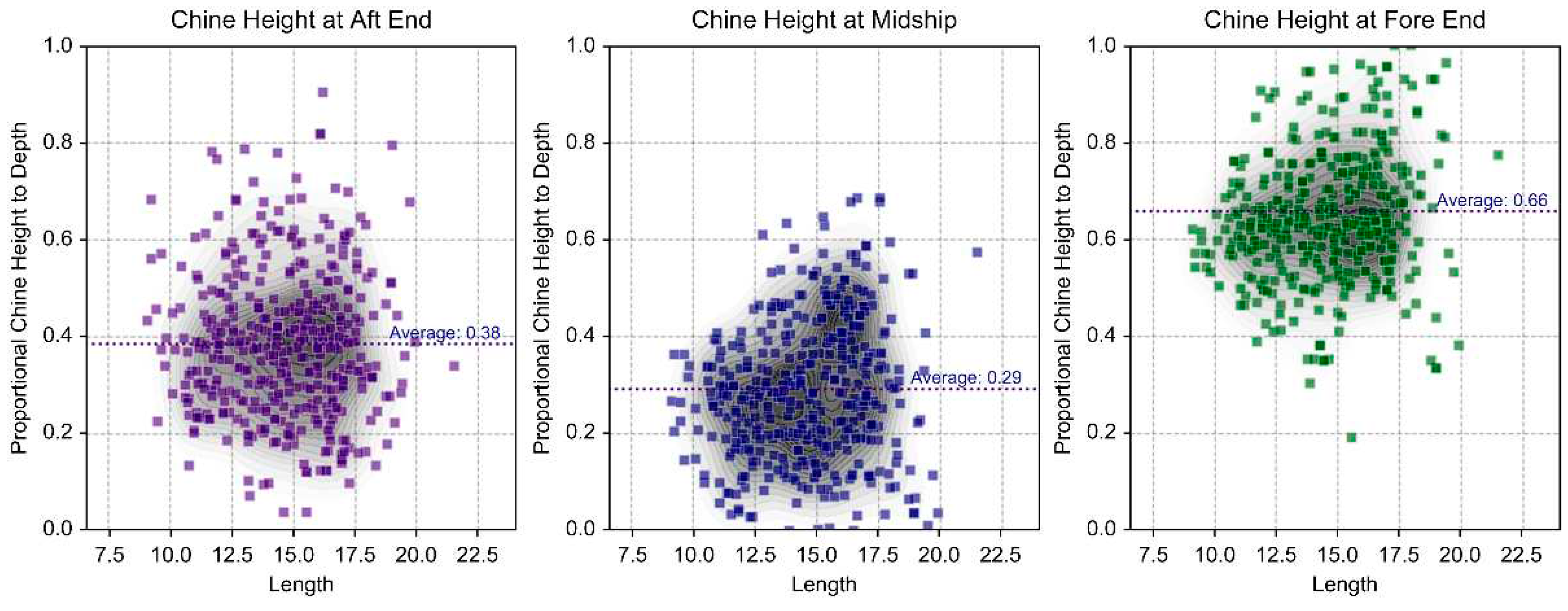
As shown in Figure 6, the distribution of chine height averages 39%, 21%, and 66% of the ship’s depth at the stern, center, and bow, respectively. The average maximum width of the chine is approximately 98% of the ship’s breadth (B_m), and it was found to extend from the stern up to 72% of the ship’s length. Small ships tend to have a relatively low chine height and maximize displacement by having a chine width close to the ship’s breadth.

Most small ships are equipped with a box keel, and we observed that the shape of the hydrostatic data near the baseline changes depending on the placement of the box keel. The average length of the box keel installation is approximately 68% of the ship’s total length (L_t), and its average volume is 3.57% of the cubic number. It was found to be installed within a range of 25% to 92% of the ship’s length from the stern.

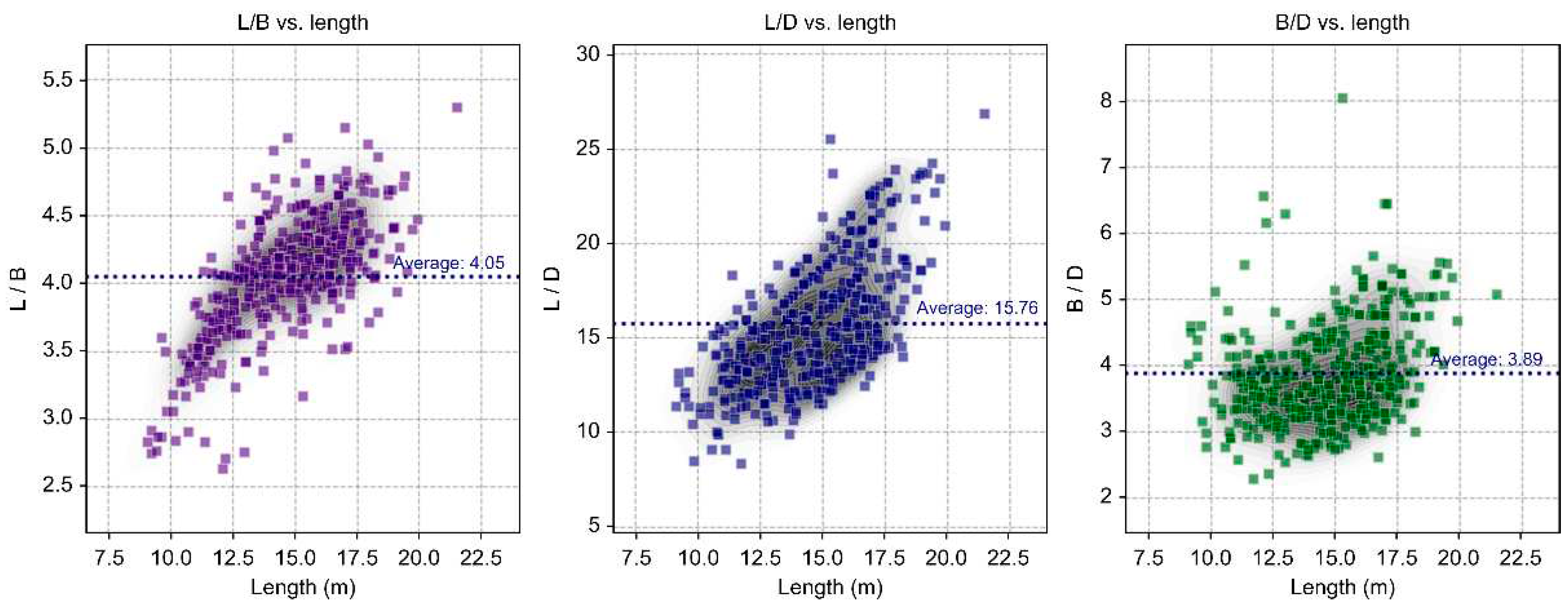
As shown in Figure 7, the distribution of key dimension ratios for small ships varies widely. In particular, the L/D ratio related to depth ranges from 8.36 to 26.88, while the B/D ratio, which is closely related to initial stability, has an average of 3.89 and a range of 2.30 to 8.05.

3.4. Deep Learning Target Data

The shape and distribution of hydrostatic data exhibit specific patterns depending on the shape and placement of the chine. By converting the form parameters that define the geometric characteristics of hydrostatic data into a mathematical model, the correlation between chine shape and form parameters can be inferred. Therefore, in this study, we converted hydrostatic data composed of continuous numerical data into a mathematical model using form parameters and set it as the target output for deep learning.

3.4.1. Mathematical Modeling Using Form Parameters

The form parameter method involves converting various types of shape data into a mathematical model by appropriately combining geometric dimensions, known as form parameters, representing the characteristics of the shape. Form parameters defining geometric characteristics consist of points (location), derivatives (slope, curvature), and integrals (area, centroid) [14].

Hydrostatic data for the 430 vessels used in the training data were calculated using a stability calculation program (K-SHIP) and are output as continuous numerical distribution-type data corresponding to draft changes.

We mathematically modeled the changes in hydrostatic data related to the underwater hull volume, location of the center of buoyancy (KB), and transverse moment of inertia according to the draft required for initial stability calculations.

In this study, we calculated form parameters by setting the hydrostatic data as a combination of second- and third-degree polynomial functions or linear functions. We then compared the errors between these mathematical models and the actual values to verify the model’s suitability.

3.4.2. Volume & KB Data Mathematical Modeling

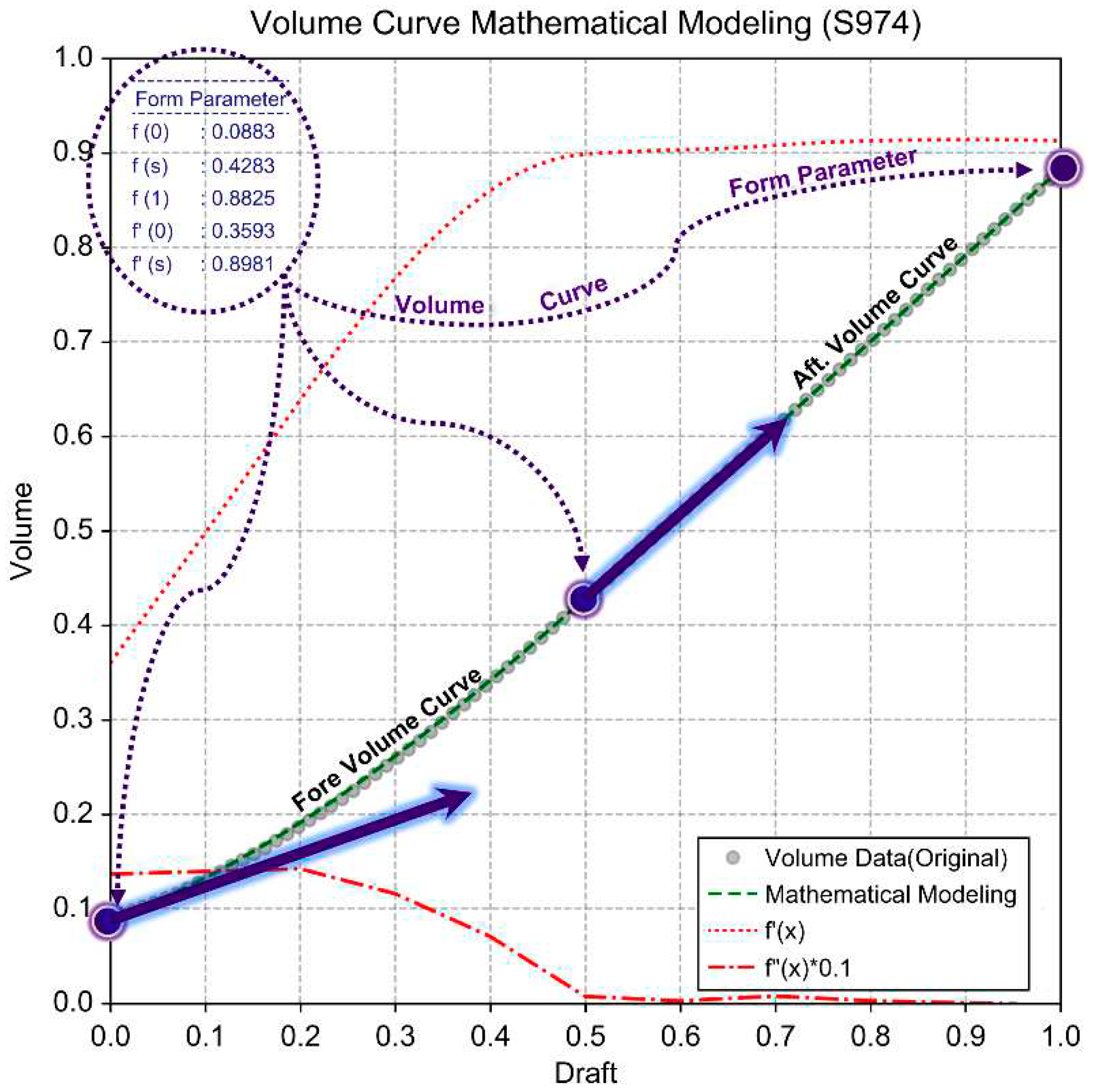
The distribution of volume data can be approximated as a curve using a polynomial function of at least a second degree with respect to draft

(x)

, as shown in Figure 8. We performed B-spline curve fitting (order=3) on the volume data, and observed that a section where the slope of fitting curve becomes constant tend to begin around 0.5D_m.

This characteristic is presumed to occur based on the location of the previously discussed chine height distribution. Generally, characteristics of the volume curve change based on this factor. Therefore, to improve the accuracy of the mathematical model transformation and learning efficiency, we set

x = 0.5

as the segment split point for mathematical modeling. We modeled the volume data as a combination of two polynomial curves based on form parameters.

V o l u m e D a t a \approx f (x) \{\begin{matrix} f_{f} (x) 0.0 \leq x \leq 0.5 \\ f_{a} (x) 0.5 < x \leq 1.0 \end{matrix}

From the B-spline fitting curve, we calculated the position and derivative form parameters (

f (x)

f^{'} (x)

) at both endpoints and the split point. We mathematically modeled the volume data as split curves of third- and second-degree polynomial functions in the fore and aft sections, applying C¹ continuity (differentiability) conditions at the split point.

Fore curve : f_{f} (x) ⇔ [f (0.0), f^{'} (0.0), f (0.5)] & polynomial degree = 3

Aft curve : f_{a} (x) ⇔ [f (0.5), f^{'} (0.5), f (1.0)] & polynomial degree = 2

We reconstructed KB data in a similar manner using a mathematical polynomial function based on form parameters and evaluated the accuracy by calculating mean absolute error (MAE), mean absolute percentage error (MAPE), and R² (R-squared score).

3.4.3. It Data Mathematical Modeling

It data represents the transverse moment of inertia (m⁴) with respect to the ship lengthwise central axis of the water plane and significantly impacts the height of the transverse metacenter, which determines the initial stability of the vessel.

As a result, the shape of the water plane varies according to the arrangement of the chine line, and It is determined according to the shape of water plane, which in turn affects the computation of the initial stability.

Small ships predominantly feature a relatively low chine height and wide chine width close to the breadth of the vessel. These ships demonstrate rapid changes in the water plane shape depending on draft changes from the baseline to the chine height. Changes in It data according to variations in chine height of the datasets used for learning were categorized into four major stages of change.

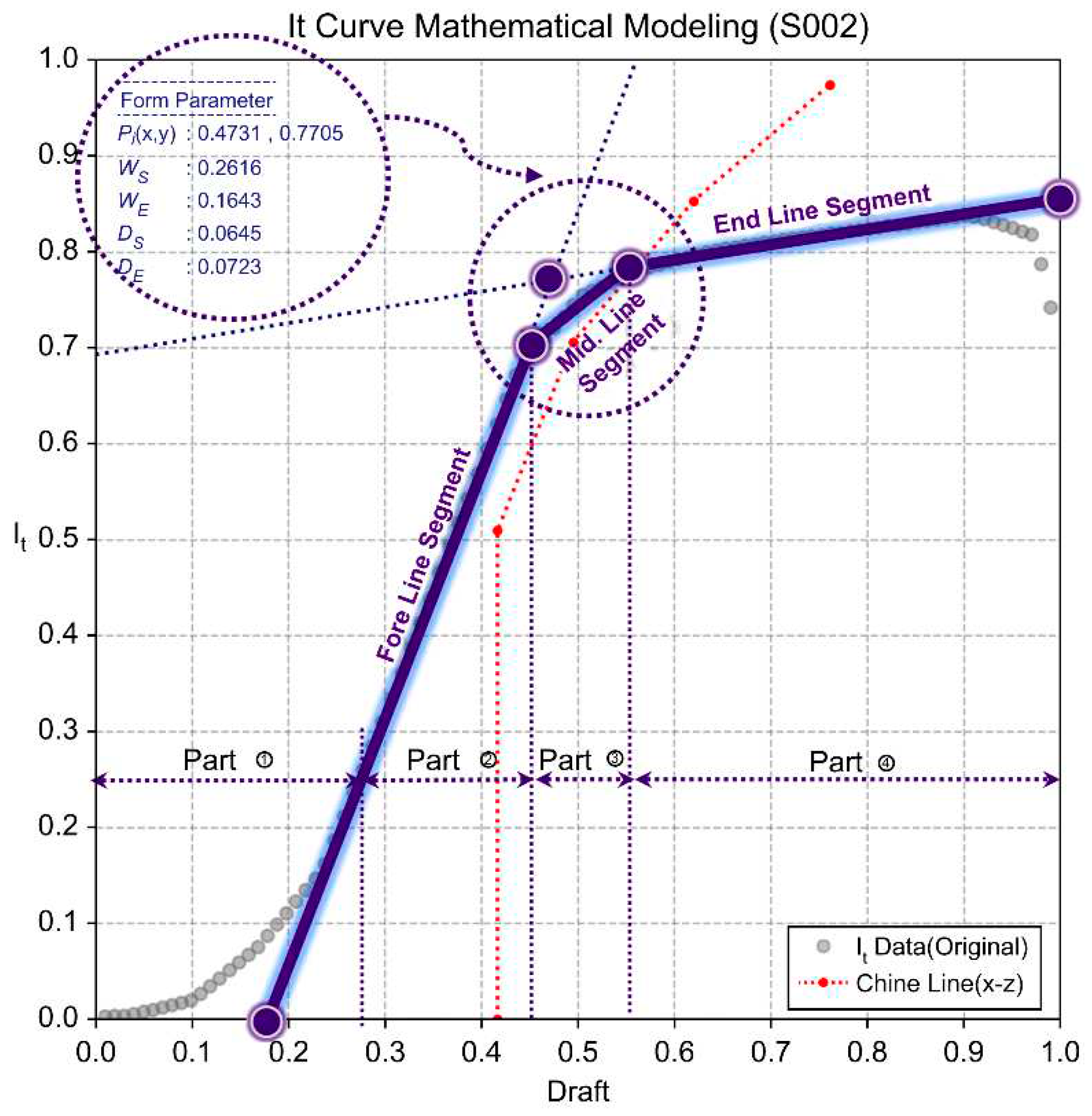
As shown in Figure 9, the stages of change in It data include a nonlinear section (Part ①), which occurs due to drastic changes in water plane shape from the baseline to the height around the central chine height caused by hull curvature. This is followed by a linear section (Part ②) extending to the maximum chine breadth height, a nonlinear section (Part ③) up to the stern chine height, and a linear section (Part ④) influenced by the final bow chine height.

In this study, considering the operational draft range of small ships, the initial nonlinear section (Part ①) was excluded. We simplified the mathematical modeling of the remaining sections of It data using a combination of three straight-line segments (fore, mid, and end line segments) with linear approximation techniques. We found that the slope and position of these line segments vary depending on the chine distribution. To simplify the mathematical model’s structure while considering the geometric distribution features of these line segments, we used their intersection points (P_ix, P_iy), weight (W_S, W_E), and intersection distance with the central segment (D_S, D_E) as form parameters in our learning data.

3.4.4. Mathematical Model Test Results

To verify the effectiveness of the mathematical model, error calculations were performed using MAPE and MAE, which are commonly used as performance metrics in regression models.

MAPE, MAE, and R² are representative performance metrics for evaluating the accuracy of the predicted model. For n data points, when comparing the model’s predicted values (

y_{i}

) to the actual values (

f (x_{i})

), MAE represents the average of all absolute errors, while MAPE shows the average percentage of absolute errors relative to the actual values. R² indicates how well the independent variable in the model can represent the dependent variable and is defined as follows.

M A E = \frac{1}{n} \sum_{i = 1}^{n} | y_{i} - f (x_{i}) |

M A P E = \frac{100}{n} \sum_{i = 1}^{n} | \frac{y_{i} - f (x_{i})}{y_{i}} | (y_{i} \neq 0)

R^{2} = \sum_{i = 1}^{n} (\frac{f (x_{i}) - \bar{y}}{y_{i} - \bar{y}})^{2} = 1 - \sum_{i = 1}^{n} (\frac{y_{i} - f (x_{i})}{y_{i} - \bar{y}})^{2}

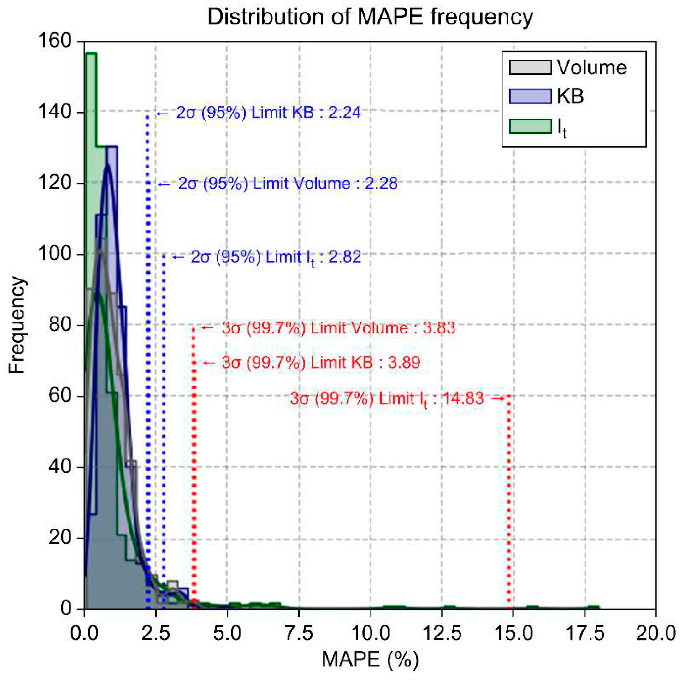
The MAPE (%) of the mathematical model ranges as 1.00–1.12%. Although some datasets showed a maximum MAPE error ranging from 3.94% to 17.96%, this likely occurs due to the nature of MAPE calculations, where the MAPE value tends to diverge toward infinity as the actual value (

y_{i}

) approaches zero.

MAE was calculated for both the real hydrostatic data (MAE^R) and the dimensionless hydrostatic data (MAE^N). The overall average MAE^R for the actual volume data was calculated to be 0.116 m³. The error ranged from a minimum of 0.009 m³ to a maximum of 0.427 m³. The overall average MAE^N for dimensionless data was calculated to be 0.22% of the cubic number. For the actual KB data values, the MAE^R ranged from a minimum of 0.001 m to a maximum of 0.007 m, with an overall average calculated to be 0.002 m. The overall average of MAE^N for dimensionless data was calculated to be 0.24% of the ship’s depth (D_m). For the actual It data values, the overall average MAE^R was calculated to be 0.324 m⁴. The error ranged from a minimum of 0.023 m⁴ to a maximum of 4.837 m⁴ (refer to Table 4).

The frequency distribution of MAPE (%) for the mathematical transformation model is illustrated in Figure 10. Some datasets had MAPE values classified as statistical outliers, and these were reviewed considering statistical heuristics. The upper limits for 2σ (95%) are a maximum error rate of 2.28%, 2.24%, and 2.82% for volume, KB, and It data, respectively. For 3σ (99.7%), the upper limits are calculated to be a maximum of 3.83%, 3.89%, and 14.83%. Within the 2σ and 3σ ranges, the overall average error rates are a maximum of 2.45% and 7.52%, respectively. The model aligns with at least 97.55% and 92.48% of the total training data within the ranges of 95% and 99.7%, respectively. The overall average MAPE of the mathematical model is 1.04%, and it was calculated that the model shows an average alignment of about 99% with the raw data.

The overall average R² for the actual values in the mathematical model is 0.9934. The average R² for It data was the lowest, calculated to be 0.9875, while for volume and KB, it was calculated to be 0.9961 and 0.9967, respectively. The coefficient of determination R², which quantifies the degree of causal relationship between variables in the regression model, is a measure that evaluates how well the independent variable represents the dependent variables and falls within the range [0, 1]. The closer R² is to 1, the higher the correlation of the independent variable with the dependent variables in the regression model. The mathematical model using the form parameter was found to have a significant correlation.

Therefore, we comprehensively examined the error rate of the mathematical transformation model using various evaluation metrics. We found that the accuracy of the model using the form parameter is satisfactory and used it as training data for deep learning.

3.5. Data Normalization

Data scaling was performed to minimize the distortion effects caused by varying numerical ranges in the training data and to enhance the efficiency and effectiveness of the learning process. Normalization¹ was carried out as described below to ensure that the learning model was not dependent on specific data and to maintain a consistent range for the weights and biases in the activation functions. Positive learning outcomes were confirmed in the deep learning model constructed for this study.

4. Composition of Deep Learning Model & Test Results

4.1 Composition of Deep Learning Model

To create and train the deep learning model, we used the Keras Model, a high-level API from the open-source library TensorFlow. For data preprocessing, numerical operations, and evaluation of learning, we utilized Python-based modules such as Pandas, NumPy, and Scikit-learn.

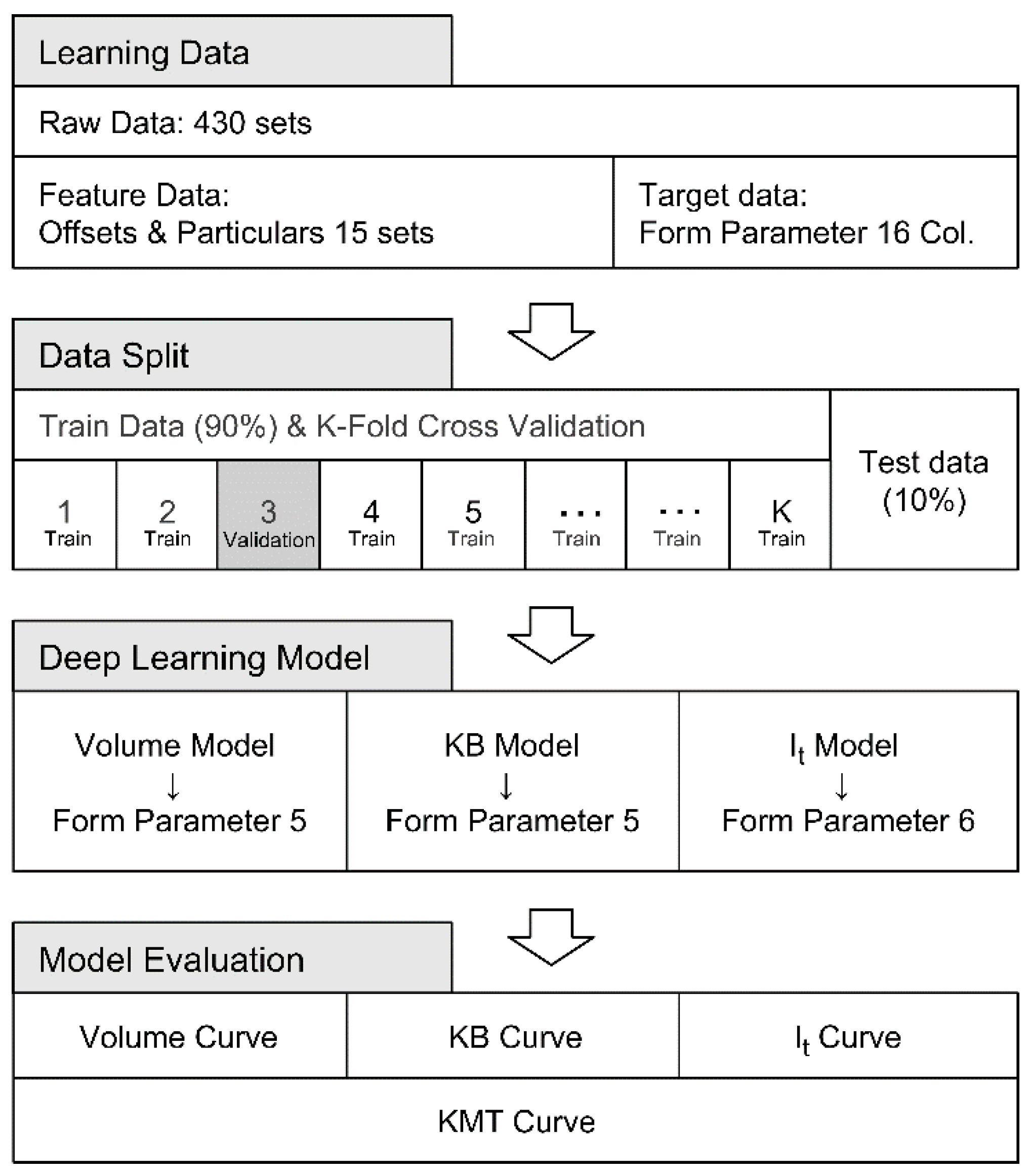
As shown in Figure 11, we designated 12 hull form feature offset data and key dimension ratios, discernible from the general arrangement of 430 vessels in the training data, as the input features for deep learning. The form parameter, calculated during the mathematical modeling process, was set as the target data for the deep learning model.

The split ratio between training and test data was set at 10%, and the data were randomly selected. To prevent overfitting and improve the model’s accuracy, K-fold cross-validation was performed on the training data. The learning rate, number of epochs, and configuration and connectivity of the hidden layers and nodes were determined through hyperparameter tuning to achieve optimal values. The activation functions used in the model include sigmoid, ELU (exponential linear unit), and ReLU (rectified linear unit), which are suitable for regression models.

Separate deep learning models were constructed for volume, KB, and It data. These models were validated by calculating the error between the mathematical model, which applied the predicted form parameter from the test data, and the actual values.

4.2. Deep Learning Test Results

Given the challenging nature of quantitatively comparing form parameter data characteristics, we evaluated the deep learning training outcomes based on MAE and the ratio (%) of MAE to the average of the actual values of form parameters in the test data (refer to Table 5). Additionally, we indirectly assessed the similarity in data distribution by comparing the item-specific ratios (%) of the descriptive statistics (mean, standard deviation, quartiles, and maximum and minimum values) between the test and predicted data.

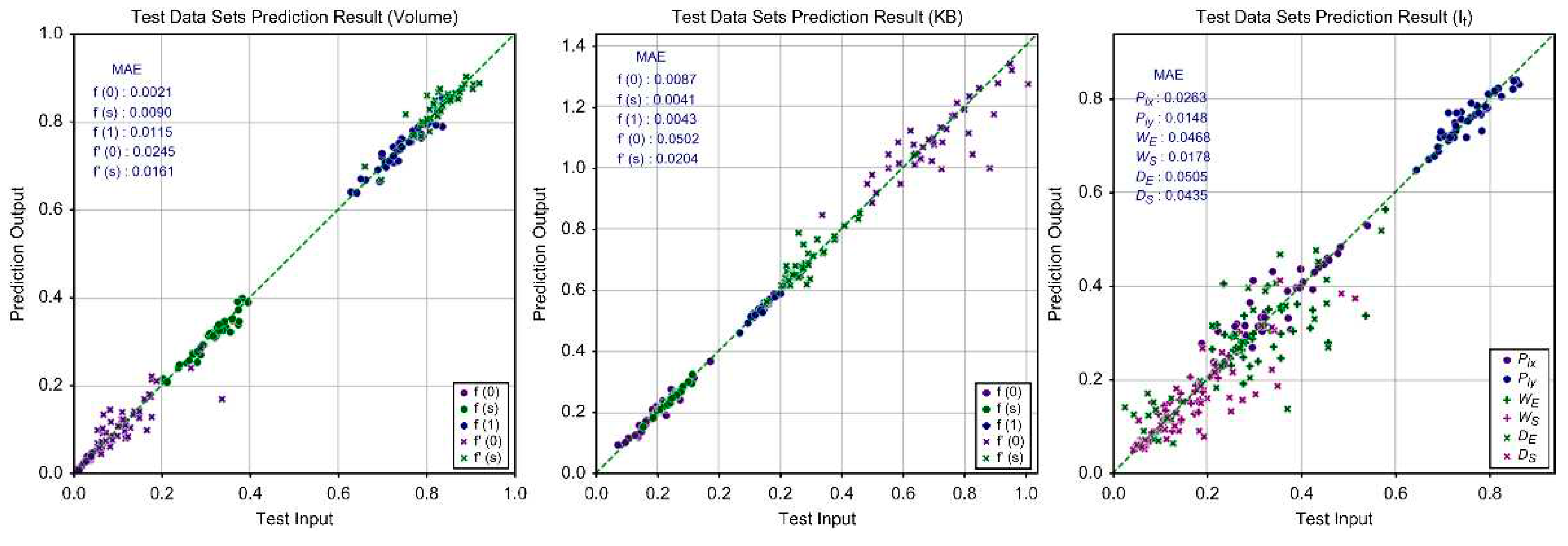
As shown in Figure 12, form parameters of volume and KB data, which show relatively consistent patterns in response to chine changes, tend to cluster closely around the equal line (

y = x

). These also demonstrated relatively low MAE percentages. However, It data, which is highly sensitive to changes in chine shape, exhibited less clustering density around the equal line and higher MAE percentages.

The overall average MAE of the predicted data is 0.0280. Compared to the average standard deviation (0.0818) of the test data, this represents approximately 34%, and the overall MAE percentage was calculated to be 7.61%.

The volume and KB curves, which exhibit consistent patterns according to draft and are mathematically modeled using a combination of polynomial functions, showed relatively satisfactory training results. In contrast, It data, modeled as a mathematical combination of multiple line segments for linear approximation, displayed inferior training results.

To examine the statistical distribution similarity between the test and predicted data, we performed mutual comparison calculations on the descriptive statistics of each dataset, as shown in Table 6, Table 7 and Table 8.

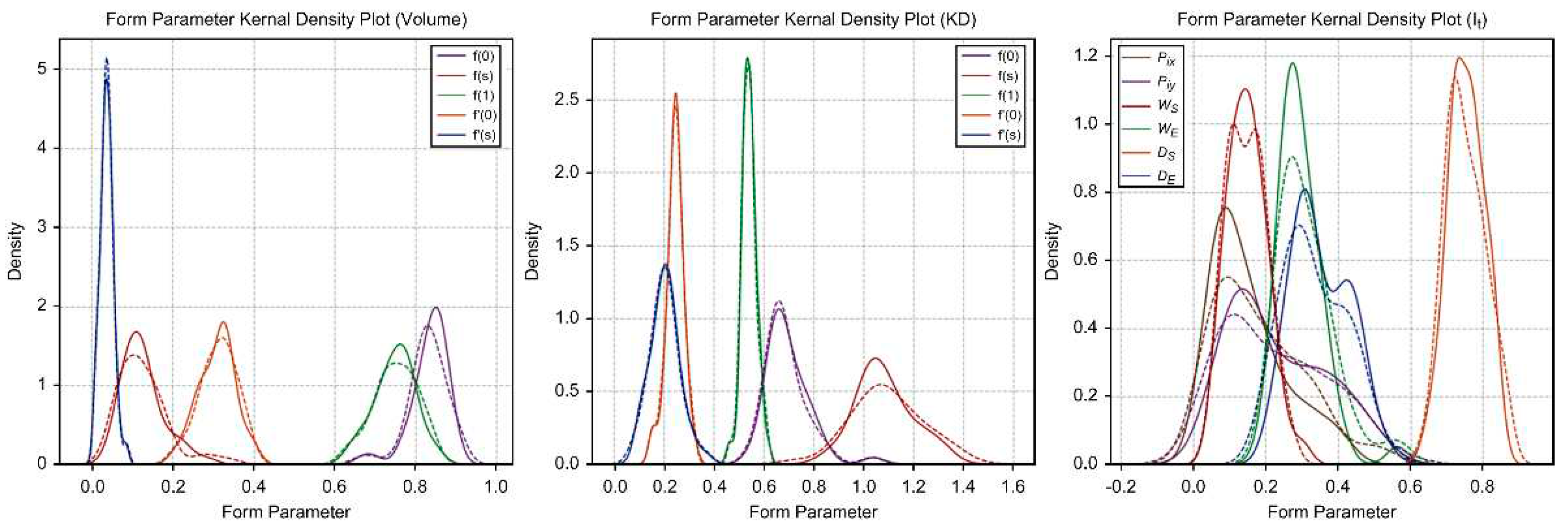
The average percentages of item-specific statistics for form parameters in the test and predicted data are as follows: volume, 101.73%; KB, 99.53%; and It, 100.88%. The overall average was calculated to be 100.74%. Kernel density estimation was conducted on the form parameters, as shown in Figure 13, to intuitively examine the similarity in data distribution trends. Based on these findings, we concluded that the test and predicted data have a significant degree of statistical distribution similarity.

Therefore, the deep learning model’s training results are considered to be relatively satisfactory. This conclusion was reached after cross-validating statistical similarities between the test and predicted data, considering data distribution forms through kernel density estimation, and calculating evaluation metrics such as MAE and MAE percentages.

4.3. Hydrostatic Data Mathematical Modeling Results

To verify the hydrostatic data mathematically modeled through deep learning, commonly used regression model evaluation metrics such as MAPE, MAE, and R² were utilized. The average MAPE for each item in the predicted data ranged from 2.54% to 2.91%, with an overall average of approximately 2.80% (refer to Table 9).

In evaluating the correlation between input and output variables in the regression model, the R² values were calculated as follows: 0.9919 for volume data and 0.9955 for KB data. These were modeled as combinations of polynomial functions. For It data, which was modeled as a mathematical combination of multiple line segments for linear approximation, a relatively low R² value of 0.8903 was observed. This also impacted the R² value for KMT ²data (0.9419). Nonetheless, the overall average R² was calculated to be 0.9549, confirming a significant correlation between input and output data.

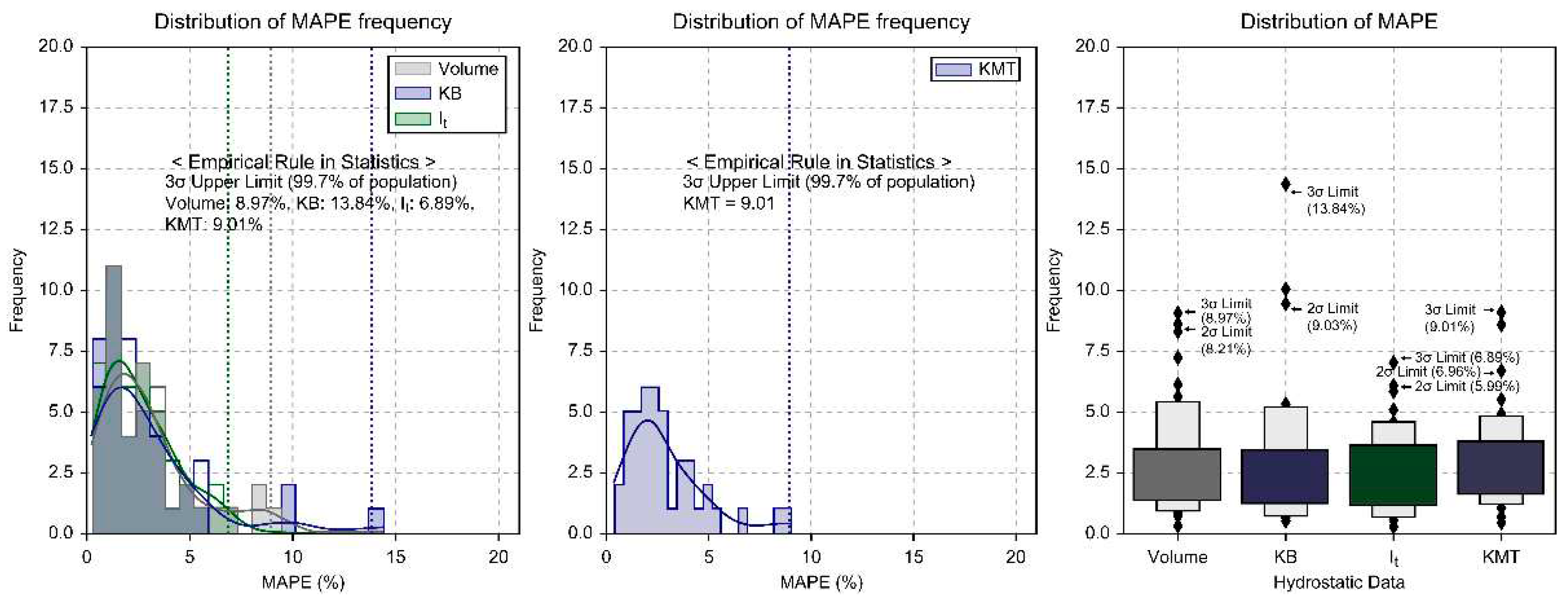
As shown in Figure 14, examining the error distribution (MAPE) of the hydrostatic data inferred through deep learning reveals that the KMT MAPE showed less than a 5% error in 91% (39 vessels) of the test data. According to the statistical empirical rule, a review of the 3σ range showed that a maximum error rate of 13.84% (KB) was observed in 99.7% of the population. The remaining items exhibited a maximum error rate calculated between 6.89% and 9.01%.

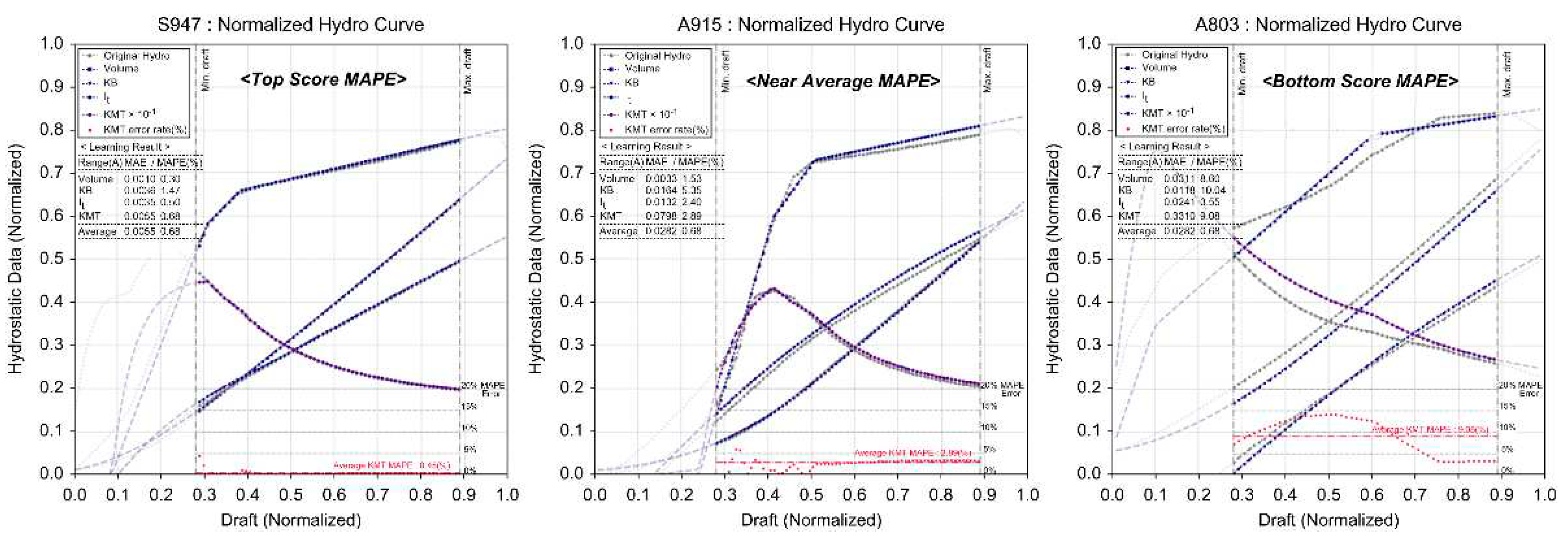
As shown in Figure 15, using the hydrostatic data inferred through deep learning for initial stability calculations on KMT data, the error rate (based on MAPE) ranged from a minimum of 0.45% to a maximum of 9.08%. The average error rate was calculated to be 2.91%, showing an alignment of over 97%. Therefore, the inference results of the hydrostatic data through deep learning proposed in this study were found to be a relatively satisfactory and reliable model. 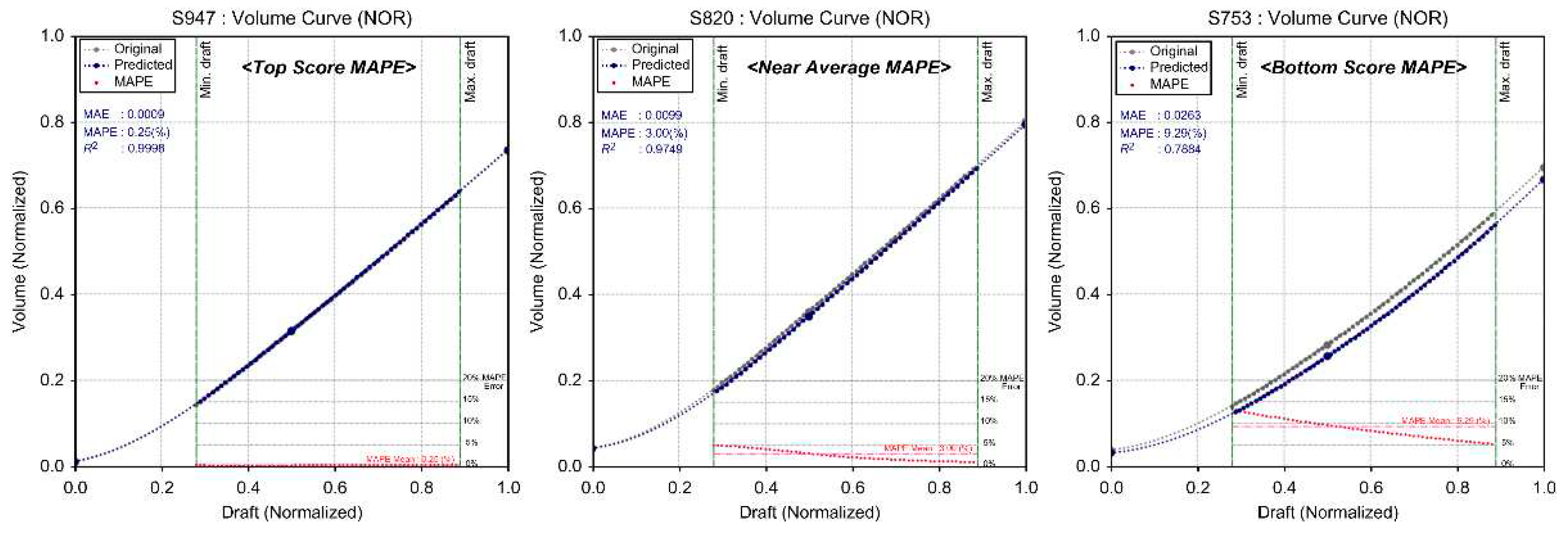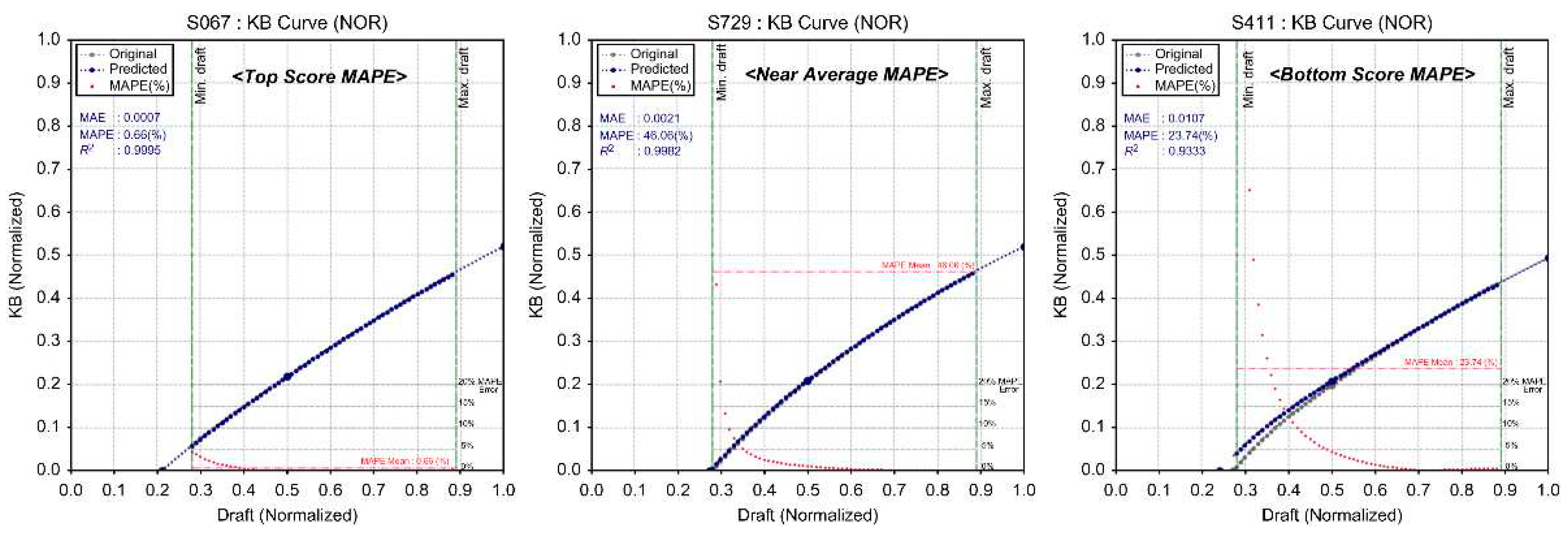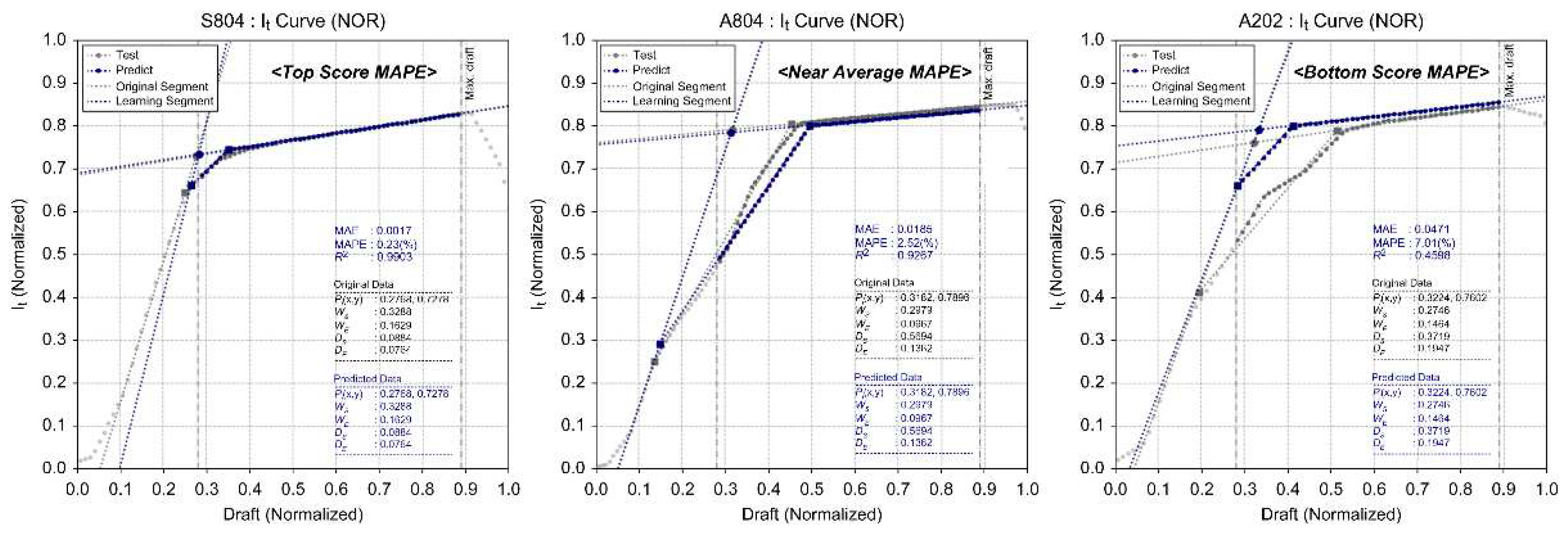Figure 16, Figure 17, Figure 18 and Figure 19 show samples of learning results.

5. Conclusion and Future Work

In this study, we set hull form feature data, which can be extracted from the general arrangements of small chine-type ships, as input variables. We then inferred the hydrostatic data needed for initial stability calculations using a multilayer neural network-based deep learning model. The following results were observed:

Hydrostatic data based on form parameters can be converted into a mathematical model.
Hydrostatic data required for initial stability calculations can be inferred by training a deep learning model using hull form feature data identifiable from general arrangements.
The deep learning model implemented in this study yielded an MAPE of 2.91% for KMT (transverse metacentric height), confirming satisfactory results.

Thus, this study confirmed the feasibility of inferring hydrostatic data needed for initial stability calculations via deep learning using limited design data (general arrangements) from small ships. By securing more real-world ship data, enabling type-specific supervised learning focused on chine shape and location, and conducting further research on hydrostatic data items, we expect the applicability of this foundational data for stability calculations in domestic coastal areas to increase further.

Author Contributions

Conceptualization: D.L., S.S.; Data curation: D.L., C.L., S.O., M.K.; Investigation: D.L., S.S.; Methodology: D.L.; Software: D.L., Validation” C.L., S.O., M.K., J.P.; Writing - review & editing: J.P.; Funding acquisition: S.S.; Project administration: S.S.; Supervision: S.S.

Funding

This work was supported by the Korea Institute of Energy Technology Evaluation and Planning (KETEP) and the Ministry of Trade, Industry & Energy (MOTIE) of the Republic of Korea (No. 20224000000090), and the Korea Institute of Marine Science & Technology Promotion (KIMST) funded by the Ministry of Oceans and Fisheries, Korea (20220210).

1	Min-Max Scaling: All feature data are transformed to be positioned between [0, 1].
2	KMT : Transverse Metacenter Height ( $\bar{K B}$ + $\bar{B M}$ ).

Institutional Review Board Statement

No applicable.

Informed Consent Statement

Not applicable.

Data Availability Statement

Not applicable.

Conflicts of Interest

The authors declare no conflict of interest.

References

Kim, T. Integrated CAD/CAE system for planning hull form design. Thesis, Pukyong National University, 2002.
Kim, I.; Go, D.; Park, D. A study on hull form design for small fishing vessels. J. Kor. Soc. Mar. Eng. 2017, 41, 316–322. [Google Scholar]
Jung, U.; Park, J.; Koo, J. Hull form development of small-size coastal leisure boat-resistance performance at high speed ranges. In Proceedings of the Korea Committee for Ocean Resources and Engineering Conference, 2003, 2003.10a, 60–63.
KOMSA, Final report on the study of expanding practical stability checks for the enhancement of fishing vessel safety. MOMAF Report, 2020.
Oh, K,; Im, N. Analysis of Domestic Fishing vessel stability regulations and research on their criteria amendment for improvement. J. Kor. Soc. Mar. Environ. Safety 2022, 28, 290–296. [Google Scholar] [CrossRef]
Kim, J.; Choi, J.; Oh, J. A study on the resistance characteristics of leisure boat according to chine shape. J. Kor. Soc. Mar. Environ. Safety 2017, 23, 566–573. [Google Scholar] [CrossRef]
Lee, G. A study on the estimation method of EHP of Small fishing boats having chine line and optimization technique of hull form parameters having low resistance. J. Kor. Soc. Fish. Ocean Technol. 1994, 30, 341–349. [Google Scholar]
Kim, J. A study for stability criteria of small fishing vessel. Thesis, Chosun University, 1999.
Oh, S.; Kang, J.; Lim, C.; Park, B.; Park, K.; Kim, H.; Shin, S. Inverse design of stern shape using a convolutional neural network. In Proceedings of the Annual Autumn Conference, The Society of Naval Architects of Korea, Gyeongju, 24-25 October, 2019, 347-351.
Kim, B. Development of a prediction system for shell plate forming information based on machine learning. Thesis, Seoul National University, 2020.
Kim, G.; Ban, I.; Park, B.; Oh, S.; Lim, C.; Shin, S. Estimation of lightweight in the initial design of ships using deep neural networks. J. Kor. Inst. Intell. Syst. 2019, 29, 416–423. [Google Scholar]
Jang, M.; Kim, D.; Zhao, Y. A study on estimating the main dimensions of a small fishing boat using deep learning. J. Kor. Soc. Fish. Ocean Technol. 2022, 58, 272–280. [Google Scholar] [CrossRef]
Chon, H.; Noh, J. Deep learning based distress awareness system for small boat. IEMEK J. Embed. Sys. Appl. 2022, 17, 281–288. [Google Scholar]
Park, W.; Shin, S.; Kim, S.; Jang, H. Preliminary hull form design using form parameter method and neural networks. J. Ocean Eng. Technol. 1999, 13, 174–181. [Google Scholar]

Figure 1. Rates of Casualty and Incident Occurrence by Marine Accident.

Figure 2. Conceptual Diagram of the Research.

Figure 3. Initial Ship Stability Calculation.

Figure 4. Concept of Dimensionless Training Data.

Figure 5. Draft Distribution in Loading.

Figure 6. Distribution of Chine Height by Ship Length.

Figure 7. Distribution of Key Dimension Ratios by Ship Length.

Figure 8. Mathematical Modeling of Volume Data.

Figure 9. Mathematical Modeling of It Data.

Figure 10. Distribution of MAPE in Mathematical Modeling.

Figure 11. Composition of Deep Learning Model.

Figure 12. Distribution of Deep Learning Training Results.

Figure 13. Kernel Density Estimation of Input and Output Form Parameters.

Figure 14. Statistical Distribution of Error (MAPE) for Hydrostatic Curve Deep Learning Results.

Figure 15. MAPE-based Hydrostatic Curve Deep Learning Results.

Figure 16. Volume Curve Deep Learning Results.

Figure 17. KB Curve Deep Learning Results.

Figure 18. It Curve Deep Learning Results.

Figure 19. KMT Curve Deep Learning Results.

Table 1. Range of Dimensionless Data.

Feature Data (Unit)		Dimensionless Scaled by	Remarks
Offset Data (m)	Length (x)	L_T (Upper Deck Length)	At aft end, value is 0
	Breadth (y)	B_m (Molded Breadth)	At centerline, value is 0
	Depth (z)	D_m (Molded Depth)	At baseline, value is 0
Volume (m³)		L_T × B_m × D_m (Cubic Number)	-
KB (m)		D_m (Molded Depth)	At baseline, value is 0
It (m⁴)		L_T × B_m³/12 (Rectangle I)	-

Table 2. Draft and Displaced Volume Statistics.

Items Statistics	Draft		Volume
Items Statistics	Min.	Max.	Min.	Max.
Mean	0.4896	0.6538	0.2899	0.4294
Standard Deviation	0.0804	0.0898	0.0577	0.0872
Min. Value	0.2405	0.3778	0.1517	0.2418
25th Percentile	0.4369	0.5898	0.2515	0.3692
50th Percentile	0.4915	0.6521	0.2870	0.4207
75th Percentile	0.5442	0.7116	0.3273	0.4796
Max. Value	0.7950	0.9250	0.4588	0.7835

Table 3. Composition of Input Data.

Items Particulars & Offsets	Description	No.
Principal Dimension Ratio	L/B, B/D, L/D	3
Principal Particulars	Aft & Fore Sheer Height	2
Upper Deck Offsets	Aft End, Midship, Max. Breadth End Offsets	3
Chine Offsets	Aft End, Midship, Max. Breadth End, Fore End Offsets	4
Box Keel Offsets	Max. Height & Offsets, Aft & Fore End Offsets	3

Table 4. Distribution of Errors in Mathematical Modeling.

Hydro. Data Error Statistics	Volume Curve				KB Curve				It Curve
Hydro. Data Error Statistics	MAPE (%)	MAE^N (-)	MAE^R (m³)	R² (-)	MAPE (%)	MAE^N (-)	MAE^R (m)	R² (-)	MAPE (%)	MAE^N (-)	MAE^R (m⁴)	R² (-)
Mean	1.00	0.0022	0.1164	0.9961	1.12	0.0024	0.0023	0.9967	1.01	0.0048	0.3235	0.9875
Standard Deviation	0.69	0.0011	0.0771	0.0040	0.63	0.0011	0.0011	0.0034	1.71	0.0044	0.4281	0.0268
Min. Value	0.08	0.0002	0.0091	0.9774	0.19	0.0006	0.0006	0.9765	0.07	0.0005	0.0230	0.5754
25th Percentile	0.51	0.0013	0.0600	0.9946	0.72	0.0016	0.0015	0.9960	0.33	0.0022	0.1036	0.9871
50th Percentile	0.88	0.0022	0.1043	0.9974	1.00	0.0022	0.0021	0.9978	0.54	0.0035	0.1949	0.9943
75th Percentile	1.37	0.0030	0.1503	0.9989	1.36	0.0030	0.0028	0.9988	0.93	0.0054	0.3677	0.9978
Max. Value	3.94	0.0058	0.4269	1.0000	4.97	0.0069	0.0066	0.9998	17.96	0.0450	4.8369	0.9999
Remark : Verification range: 0.28d to 0.89d, frequency: 430 vessels

Table 5. Error Distribution of Deep Learning Training Results.

Items	Error Target Data	MAE	Test Data Average	Error Rate (%)
Volume	$f (0)$	0.0021	0.0383	5.53
	$f (s)$	0.0090	0.3132	2.88
	$f (1)$	0.0115	0.7509	1.53
	$f^{'} (0)$	0.0245	0.1280	19.16
	$f^{'} (s)$	0.0161	0.8291	1.94
	Average	0.0127	0.4119	6.21
KB	$f (0)$	0.0087	0.2038	4.28
	$f (s)$	0.0041	0.2445	1.69
	$f (1)$	0.0043	0.5412	0.80
	$f^{'} (0)$	0.0502	1.0953	4.58
	$f^{'} (s)$	0.0204	0.6898	2.95
	Average	0.0175	0.5549	2.86
It	$P_{i x}$	0.0263	0.3369	7.80
	$P_{i y}$	0.0148	0.7526	1.97
	$W_{S}$	0.0468	0.3153	14.84
	$W_{E}$	0.0178	0.1480	12.04
	$D_{S}$	0.0505	0.2279	22.18
	$D_{E}$	0.0435	0.1825	23.82
	Average	0.0333	0.3272	13.77

Table 6. Comparison of Input and Output Statistical Measures for Volume Curve Form Parameter.

Target Data Statistics	$f (0)$		$f (s)$		$f (1)$		$f^{'} (0)$		$f^{'} (s)$
Target Data Statistics	Test	Predict	Test	Predict	Test	Predict	Test	Predict	Test	Predict
Mean	0.0383	0.0385	0.3132	0.3101	0.7509	0.7489	0.1280	0.1269	0.8291	0.8341
Standard Deviation	0.0156	0.0158	0.0453	0.0443	0.0535	0.0504	0.0614	0.0517	0.0499	0.0464
Min. Value	0.0094	0.0096	0.2040	0.2093	0.6296	0.6396	0.0565	0.0456	0.6608	0.6689
25th Percentile	0.0304	0.0302	0.2837	0.2766	0.7202	0.7162	0.0837	0.0937	0.8068	0.8131
50th Percentile	0.0378	0.0371	0.3168	0.3156	0.7427	0.7545	0.1174	0.1190	0.8317	0.8428
75th Percentile	0.0458	0.0475	0.3411	0.3374	0.7882	0.7812	0.1555	0.1429	0.8570	0.8625
Max. Value	0.0873	0.0850	0.3962	0.3991	0.8372	0.8552	0.3375	0.2858	0.9185	0.9025

Table 7. Comparison of Input and Output Statistical Measures for KB Curve Form Parameter.

Target Data Statistics	$f (0)$		$f (s)$		$f (1)$		$f^{'} (0)$		$f^{'} (s)$
Target Data Statistics	Test	Predict	Test	Predict	Test	Predict	Test	Predict	Test	Predict
Mean	0.2038	0.2055	0.2445	0.2449	0.5412	0.5423	1.0953	1.0834	0.6898	0.6972
Standard Deviation	0.0602	0.0582	0.0348	0.0343	0.0285	0.0281	0.1415	0.1130	0.0868	0.0861
Min. Value	0.0724	0.0965	0.1547	0.1545	0.4668	0.4620	0.7347	0.8453	0.5544	0.5597
25th Percentile	0.1645	0.1726	0.2313	0.2294	0.5208	0.5252	1.0075	1.0115	0.6380	0.6428
50th Percentile	0.1996	0.2047	0.2469	0.2482	0.5434	0.5394	1.0920	1.0762	0.6710	0.6800
75th Percentile	0.2359	0.2392	0.2650	0.2661	0.5536	0.5575	1.1860	1.1503	0.7126	0.7372
Max. Value	0.3722	0.3688	0.3128	0.3244	0.6119	0.6163	1.4043	1.3396	1.0325	1.0412

Table 8. Comparison of Input and Output Statistical Measures for It Curve Form Parameter.

Target Data Statistics	$P_{i x}$		$P_{i y}$		$W_{S}$		$W_{E}$		$D_{S}$		$D_{E}$
Target Data Statistics	Test	Predict	Test	Predict	Test	Predict	Test	Predict	Test	Predict	Test	Predict
Mean	0.3369	0.3531	0.7526	0.7546	0.3153	0.2978	0.1480	0.1501	0.2279	0.2337	0.1825	0.1545
Standard Deviation	0.0868	0.0775	0.0538	0.0473	0.0806	0.0636	0.0530	0.0536	0.1422	0.1309	0.1219	0.1001
Min. Value	0.1891	0.2328	0.6441	0.6471	0.2123	0.1929	0.0512	0.0595	0.0259	0.0654	0.0439	0.0518
25th Percentile	0.2779	0.2997	0.7140	0.7198	0.2623	0.2642	0.1079	0.1126	0.1049	0.1259	0.0698	0.0725
50th Percentile	0.3182	0.3318	0.7392	0.7562	0.2917	0.2819	0.1444	0.1530	0.2114	0.1898	0.1407	0.1205
75th Percentile	0.4011	0.4218	0.7907	0.7843	0.3567	0.3285	0.1823	0.1857	0.3357	0.3399	0.2531	0.2024
Max. Value	0.5402	0.5287	0.8623	0.8392	0.5793	0.5646	0.2694	0.3022	0.5694	0.5180	0.5144	0.4131

Table 9. Error and Evaluation Metrics for Hydrostatic Curve Deep Learning Results.

Items Error Ship No	Volume Curve			KB Curve			It Curve			KMT Curve
Items Error Ship No	MAPE (%)	MAE	R²	MAPE (%)	MAE	R²	MAPE (%)	MAE	R²	MAPE (%)	MAE	R²
S947	0.30	0.0010	0.9999	1.47	0.0036	0.9979	0.50	0.0035	0.9944	0.45	0.0140	0.9984
A714	0.69	0.0023	0.9997	0.85	0.0015	0.9997	0.52	0.0041	0.9893	0.66	0.0201	0.9975
A913	1.00	0.0027	0.9995	3.21	0.0053	0.9977	1.32	0.0088	0.9846	1.01	0.0293	0.9909
S513	3.49	0.0119	0.9930	4.03	0.0086	0.9917	3.81	0.0257	0.7961	1.05	0.0278	0.9917
S720	1.22	0.0055	0.9985	2.01	0.0017	0.9997	0.27	0.0020	0.9942	1.08	0.0263	0.9975
S067	0.71	0.0027	0.9996	0.52	0.0009	0.9999	1.23	0.0092	0.9895	1.21	0.0443	0.9885
S624	1.54	0.0067	0.9979	1.92	0.0056	0.9969	0.71	0.0056	0.9692	1.29	0.0317	0.9972
S818	2.13	0.0072	0.9969	0.55	0.0017	0.9997	1.44	0.0100	0.9926	1.34	0.0333	0.9878
S763	1.44	0.0040	0.9992	1.44	0.0048	0.9977	0.57	0.0038	0.9990	1.35	0.0393	0.9867
S959	0.95	0.0034	0.9995	0.66	0.0019	0.9996	1.66	0.0113	0.9721	1.56	0.0509	0.9760
S804	1.43	0.0050	0.9989	0.72	0.0026	0.9989	0.23	0.0017	0.9903	1.56	0.0397	0.9923
S729	0.71	0.0022	0.9997	2.96	0.0050	0.9980	1.12	0.0073	0.9887	1.64	0.0441	0.9873
A923	1.56	0.0031	0.9992	2.57	0.0051	0.9981	0.68	0.0031	0.9988	1.92	0.0514	0.9661
S999	3.00	0.0091	0.9954	1.80	0.0060	0.9967	3.73	0.0265	0.9630	1.93	0.0540	0.9866
S984	4.73	0.0162	0.9865	1.27	0.0031	0.9992	2.71	0.0178	0.9710	1.99	0.0547	0.9861
S032	1.76	0.0036	0.9993	0.57	0.0013	0.9997	3.68	0.0207	0.9806	2.01	0.0517	0.9668
S023	1.31	0.0032	0.9993	1.87	0.0036	0.9986	1.11	0.0067	0.9946	2.05	0.0634	0.9612
A710	2.86	0.0101	0.9956	1.83	0.0052	0.9975	1.67	0.0114	0.9491	2.11	0.0474	0.9847
S979	2.03	0.0069	0.9976	1.44	0.0039	0.9984	1.38	0.0098	0.9781	2.25	0.0568	0.9854
A804	0.93	0.0030	0.9995	1.11	0.0029	0.9992	2.52	0.0185	0.9267	2.27	0.0833	0.9560
S648	3.16	0.0126	0.9930	1.75	0.0045	0.9981	2.11	0.0157	0.9504	2.32	0.0636	0.9722
S709	1.50	0.0045	0.9990	4.90	0.0127	0.9788	1.59	0.0102	0.9834	2.33	0.0706	0.9789
S956	3.07	0.0113	0.9933	0.52	0.0014	0.9998	2.19	0.0160	0.7036	2.34	0.0973	0.9521
S820	2.89	0.0105	0.9951	2.69	0.0077	0.9942	1.16	0.0086	0.9113	2.49	0.0588	0.9872
A914	3.07	0.0126	0.9925	5.22	0.0078	0.9959	4.38	0.0339	0.9416	2.62	0.1233	0.9427
S667	3.50	0.0107	0.9945	0.79	0.0020	0.9995	6.01	0.0418	0.7213	2.75	0.0516	0.9840
S066	2.78	0.0106	0.9947	3.04	0.0073	0.9960	2.46	0.0198	0.9126	2.82	0.1016	0.9851
A909	1.26	0.0031	0.9993	3.74	0.0088	0.9931	2.45	0.0083	0.9954	2.85	0.0774	0.9506
A915	1.53	0.0033	0.9994	5.35	0.0164	0.9812	2.40	0.0132	0.9928	2.89	0.0798	0.9834
S706	2.42	0.0074	0.9962	1.00	0.0035	0.9987	3.90	0.0205	0.9646	3.06	0.0865	0.8897
S784	0.62	0.0017	0.9998	3.14	0.0069	0.9963	3.54	0.0247	0.8437	3.56	0.0983	0.8942
S980	8.32	0.0353	0.9486	1.47	0.0041	0.9981	4.62	0.0379	0.2933	3.69	0.1111	0.9770
S411	3.72	0.0160	0.9890	14.39	0.0099	0.9867	1.14	0.0090	0.6384	3.88	0.3108	0.9622
S778	3.83	0.0137	0.9915	5.28	0.0091	0.9916	5.83	0.0409	0.5320	4.18	0.1721	0.9053
A202	2.52	0.0086	0.9968	1.18	0.0036	0.9985	7.01	0.0471	0.4598	4.20	0.1008	0.8376
S816	6.10	0.0219	0.9758	1.88	0.0054	0.9969	2.35	0.0169	0.9610	4.22	0.1208	0.9483
S702	2.62	0.0085	0.9967	3.05	0.0067	0.9954	2.12	0.0149	0.9445	4.61	0.1464	0.8863
S064	7.19	0.0294	0.9636	4.99	0.0092	0.9898	3.03	0.0219	0.5322	4.90	0.1364	0.9591
S009	1.83	0.0070	0.9958	3.57	0.0117	0.9871	6.08	0.0433	0.8645	4.94	0.1347	0.9356
S909	4.62	0.0170	0.9884	9.44	0.0124	0.9814	3.47	0.0280	0.8381	5.47	0.2559	0.9326
A606	5.57	0.0099	0.9942	1.24	0.0031	0.9992	5.07	0.0109	0.9928	6.68	0.1227	0.7573
S753	9.03	0.0290	0.9508	1.69	0.0054	0.9969	1.70	0.0106	0.9880	8.55	0.1557	0.5112
A803	8.60	0.0311	0.9507	10.04	0.0118	0.9870	3.55	0.0241	0.8971	9.08	0.3310	0.6866
Average	2.87	0.0099	0.9919	2.86	0.0057	0.9955	2.54	0.0169	0.8903	2.91	0.0900	0.9419

Disclaimer/Publisher’s Note: The statements, opinions and data contained in all publications are solely those of the individual author(s) and contributor(s) and not of MDPI and/or the editor(s). MDPI and/or the editor(s) disclaim responsibility for any injury to people or property resulting from any ideas, methods, instructions or products referred to in the content.

© 2023 by the authors. Licensee MDPI, Basel, Switzerland. This article is an open access article distributed under the terms and conditions of the Creative Commons Attribution (CC BY) license (http://creativecommons.org/licenses/by/4.0/).

Copyright: This open access article is published under a Creative Commons CC BY 4.0 license, which permit the free download, distribution, and reuse, provided that the author and preprint are cited in any reuse.

MDPI Initiatives

Important Links

Choose an area of interest and we will send you notifications of new preprints at your preferred frequency.

Disclaimer