FPGA Implementation of Complex-Valued Neural Network for Polar-Represented Image Classification

Preprint

Article

FPGA Implementation of Complex-Valued Neural Network for Polar-Represented Image Classification

Altmetrics

Downloads

Views

Comments

A peer-reviewed article of this preprint also exists.

Supplementary Material

supplementary.pdf (18.22MB )

MARUF AHMAD^*,

Lei Zhang^*

Muhammad E. H. Chowdhury

MARUF AHMAD^*,

Lei Zhang^*

Muhammad E. H. Chowdhury

This version is not peer-reviewed

Submitted:

16 November 2023

Posted:

22 November 2023

You are already at the latest version

Alerts

Abstract

This proposed research explores a novel approach to image classification by deploying a complex-valued neural network (CVNN) on a field-programmable gate array (FPGA), specifically for classifying 2D images transformed into polar form. The aim of this research is to address the limitations of existing neural network models in terms of energy and resource efficiency, by exploring the potential of FPGA-based hardware acceleration in conjunction with advanced neural network architectures like CVNNs. The methodological innovation of this research lies in the Cartesian to polar transformation of 2D images, effectively reducing the input data volume required for neural network processing. Subsequent efforts focused on constructing a CVNN model optimized for FPGA implementation, emphasizing the enhancement of computational efficiency and overall performance. The experimental findings provide empirical evidence supporting the efficacy of the image classification system developed in this study. One of the developed models, CVNN_128, achieves an accuracy of 88.3% with an inference time of just 1.6ms and a power consumption of 4.66mW for the classification of the MNIST test dataset consists of 10,000 frames. While there is a slight concession in accuracy compared to recent FPGA implementations that achieve 94.43%, our model significantly excels in classification speed and power efficiency—surpassing existing models by more than a factor of 100. In conclusion, the paper demonstrates the substantial advantages of FPGA-implementation of CVNNs for image classification tasks, particularly in scenarios where speed, resource, and power consumption are critical. The study’s reproducible results and corresponding code are available on GitHub at the following link: https://github.com/mahmad2005/CVNNonFPGA

Keywords:

Subject: Engineering - Electrical and Electronic Engineering

1. Introduction

Recently, Generative Artificial Intelligence (GAI) [1] technologies have surged to the forefront, with tools like ChatGPT [2] and AI-powered image and video generators [3] like MidJourney [4] dominating the conversation. At the core of these visual generators lies in the image processing and classification, serving as the backbone of this AI-driven revolution. These breakthroughs have been made possible by the remarkable progress in artificial neural networks applied to image and video processing [5]. However, this progress has come at the cost of increased computational complexity. The amount of layers and neurons in each layer required for state-of-the-art deep models has grown significantly, often involving millions of parameters and billions of operations to achieve human-level accuracy.

Simultaneously, the growth of Internet of Things (IoT) and embedded systems has led to an escalating demand for neural network models to perform various tasks. However, the computational demands of deep neural networks present challenges when deploying them on low-power embedded platforms with limited computational and power resources [6,7].

To address these challenges and enhance the efficiency of neural network algorithms, particularly in terms of reducing computational costs, energy consumption, and resource usage, multiple strategies have emerged. One approach focuses on reducing the theoretical number of basic operations required in neural network computations through algorithmic innovations. Simultaneously, another direction aims to improve neural network algorithms using hardware accelerators, such as ASIC and FPGA designs [6,7].

In our work, we explore both of these approaches. We present innovative image preprocessing methods tailored for neural network models and introduce a hardware accelerator model designed to reduce computational costs in neural networks and optimize energy and resource utilization in hardware systems. This research endeavors to contribute to the ongoing efforts aimed at making neural network applications more efficient and sustainable, addressing the challenges posed by increasing computational demands.

The efficacy of image classification models hinges not only on the sophistication of neural network architectures but also on the quality of the input data and the performance of the processing pipeline. Traditionally, image classification processes have operated in Cartesian coordinates (x, y), where 2D images are serialized for neural network input. However, this conventional approach poses challenges. Applying frequency analysis methods like the Fourier Transform to serialize two-dimensional (2D) images can inadvertently lead to the omission of significant spatial data. This pertains to the positional information of the pixels and the contextual interactions between neighboring pixels, which can be diminished in the serialization transition.

Recent research [8] has addressed this limitation by introducing a novel preprocessing pipeline that transforms standard image datasets into a polar coordinate representation. This transformation is inspired by the recognition that polar coordinates, defined by radial distance

(r)

and angular displacement

(θ)

from a reference point, provide a more natural representation for circular and radial patterns. This transformation effectively retains the spatial information inherent in the pixel arrangement of the original image. By encoding images in polar coordinates, it aims to exploit these advantages and enhance the classification accuracy of image datasets. However, the research has not yet ventured into the practical application of this method in real-world image classification, despite its initial focus on constructing a SNN model. To overcome the existing gap in research, our study focuses on replicating the process of converting 2D images from Cartesian to polar coordinates. Subsequently, we apply this transformation technique to the challenge of classifying the MNIST [9] handwritten digit dataset using artificial neural networks.

An essential aspect of the preprocessing pipeline involves the application of the DFT to the polar-transformed images. The DFT is a powerful mathematical tool for decomposing signals into their constituent frequency components, and it has found extensive use in image analysis. In our approach, we leverage the DFT to extract both magnitude and phase information from the polar-represented images. The utilization of complex exponentials within the DFT allows us to capture nuanced variations in pixel values and relationships, thus preserving essential spatial data.

What sets our research apart is the integration of CVNNs into the image classification framework. Unlike traditional RVNNs, CVNNs are tailored to handle complex-valued data, such as the output of the DFT. By treating the DFT outputs as complex numbers, we effectively harness the rich information embedded in both the real and imaginary parts. This nuanced approach promises to provide a more holistic understanding of the input data, potentially leading to improved classification accuracy.

While the theoretical advantages of CVNNs in image classification have been explored in the literature, there is a notable gap in the practical implementation of such networks, particularly on resource-constrained platforms. Therefore, our research extends beyond theoretical exploration to encompass practical deployment. We aim to implement the trained CVNN model on FPGA, capitalizing on the parallel processing capabilities intrinsic to FPGA architecture. The FPGA implementation offers the potential for real-time classification with significantly reduced computational resources and power requirement compared to traditional CPU-based sequential computing and GPU-based parallel computing.

1.1. Related Workd

Within the domain of image classification, conventional neural network models like Feed-Forward Neural Networks [10], CVNNs , RNNs[11], and Deep Neural Networks [12] have primarily been designed to handle real-valued data. However, the growing prevalence of complex-valued data sources [13,14,15] such as Complex-Valued MRI Images, SAR (Synthetic Aperture Radar) Images, Sonar Images, Optical Coherence Tomography (OCT) Images, as well as sound and wave signals, has spurred the need for specialized neural network models capable of directly processing complex-valued inputs. Consequently, researchers have responded by developing a range of models tailored to meet this specific demand.

As the capabilities of neural network models continue to grow in complexity, and the data they process becomes increasingly vast, the computational demands and time required for tasks have surged [6]. Consequently, there is a pressing need to discover solutions that can enhance the speed and throughput of neural networks while minimizing energy consumption. This has led to the emergence of hardware accelerators as a pivotal area of research focus [7]. Accelerators utilizing GPUs, FPGAs, and ASICs have garnered attention for their potential to meet the performance requirements of deep learning tasks. While GPU-based models have shown considerable performance, their applicability in power-sensitive embedded devices remains a challenge, primarily due to their higher energy consumption. In contrast, FPGAs have gained prominence for their remarkable energy efficiency [16,17], flexibility, and shorter development periods compared to ASICs. With robust parallel computing capabilities and reduced energy consumption, FPGAs have risen to prominence in the field of hardware acceleration for deep learning. These reconfigurable devices enable engineers to simulate digital circuits efficiently, paving the way for enhanced neural network computation. Unlike CPUs, which face inherent structural limitations when processing vast amounts of data, FPGAs offer a versatile solution with virtually limitless reconfigurable logic, enabling the creation of tailored accelerators for a multitude of applications. This inherent adaptability, combined with their capacity for parallel processing and pipeline optimization, positions FPGAs as a compelling choice for fast and energy-efficient neural network model implementations [7].

A Recent research from our lab, Zahng et al. [18] presents an energy-efficient Spiking Neural Network (SNN) designed and implemented on FPGA, emphasizing lower power consumption and minimal accuracy loss. The approach utilizes rate coding to map ANN parameters to SNNs efficiently, yielding power efficiency of 8841.7 frames/watt with minimal accuracy degradation. The system sets a new performance standard, achieving an impressive 90.39% accuracy rate, outperforming conventional SNN benchmarks.

Several studies [19,20,21] have investigated hardware accelerators for MNIST classification using neural networks, primarily centered on CNNs. These studies also provide comparisons of speed and resource utilization in contrast to CPUs or GPUs.

As of May 2023, we have identified just one instance of a CVNN model implemented on FPGA [22]. The study introduces ComplexNet, a deep convolutional CVNN for channel estimation (CE) in 5G OFDM communication systems. It demonstrates that ComplexNet enhances CE accuracy and offers a lightweight FPGA implementation, significantly reducing power consumption compared to CPU and GPU platforms.

Notably, to best of our knowledge, no prior implementations of complex-valued neural networks on FPGA for MNIST dataset classification have been found in our research.

1.2. Research Objectives

The primary goal of this research is to explore the efficacy of polar coordinate representation of 2D image data and its impact on Complex-Valued Neural Networks (CVNNs) and Real-Valued Neural Networks (RVNNs) in image classification tasks. A key focus is the comparative analysis of these neural networks in handling complex-valued inputs and the subsequent implementation on Field-Programmable Gate Arrays (FPGAs) to assess resource utilization, power efficiency, and inference speed. The goal is to demonstrate the practical advantages of FPGA acceleration for real-time image classification, thus achieving faster classification while consuming fewer resources and power.

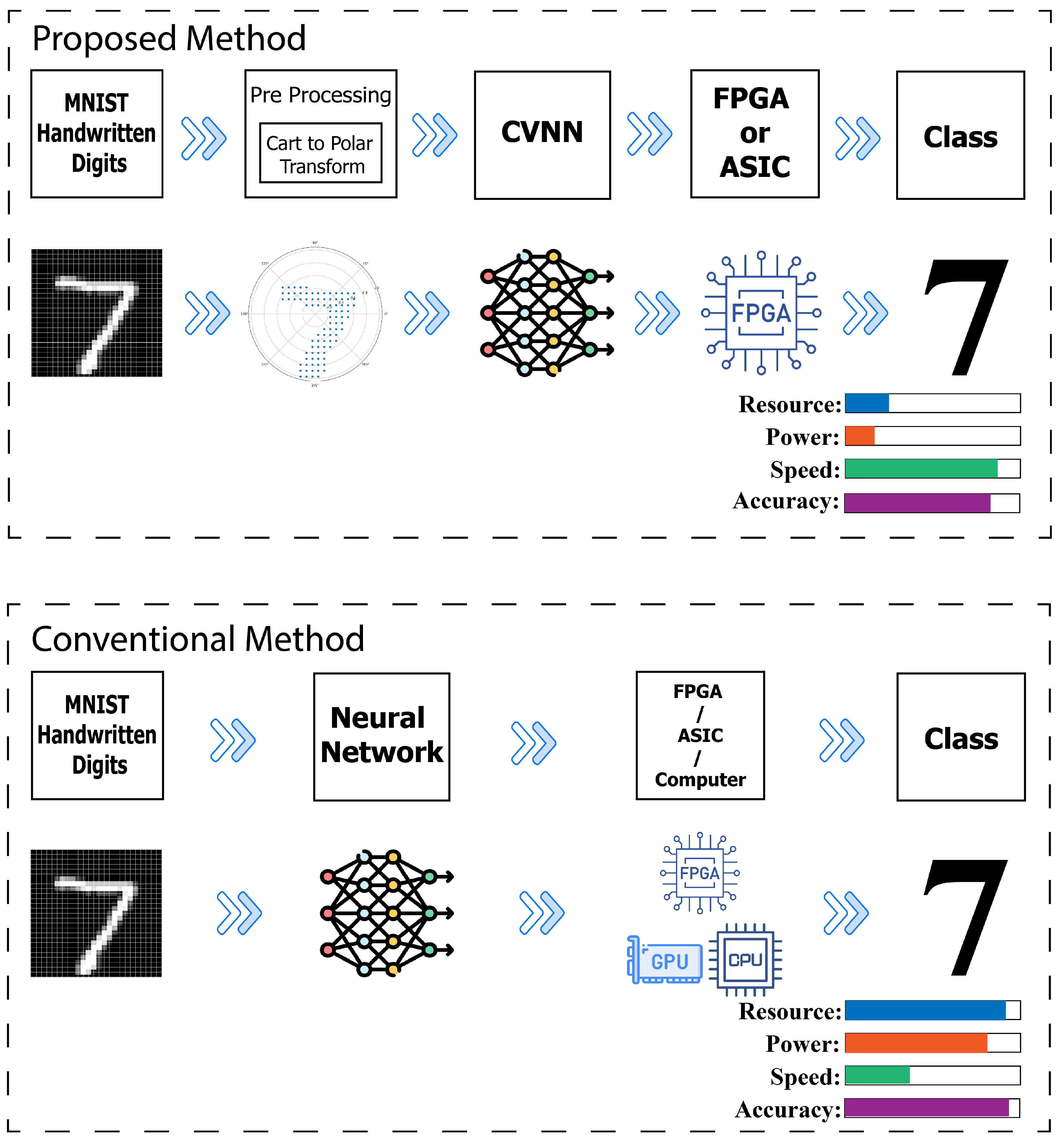
By achieving these objectives, this research seeks to contribute to the fields of image processing, neural networks, and hardware acceleration by offering a holistic approach to image classification that incorporates innovative preprocessing techniques, advanced neural network architectures, and efficient hardware deployment strategies. The main objective is to achieve image classification while also minimizing the need, for resources and power which helps tackle issues, in real time image processing applications as shown in Figure 1.

1.3. Outline

The remaining sections of the paper are organized in the way;

Section 2: In this section we provide an overview of the cartesian to polar coordinate representation for 2d images..

Section 3 and 4 : In this section we provide an account of how the CVNN’s implemented for preprocessed image data. We also compare its performance with real valued neural network counterparts.

Section 5 and 6: This section offers an explanation of how the hardware accelerator’s implemented for CVNN using FPGA. We present an analysis of its performance compared to running the model on environmental setups like CPU and GPU. We also compare it against existing research.

Section 7: The final section serves as a summary of this research. It outlines discussions highlights any limitations encountered during research suggests areas, for work and provides concluding remarks.

2. Cartesian to Polar coordinate representation

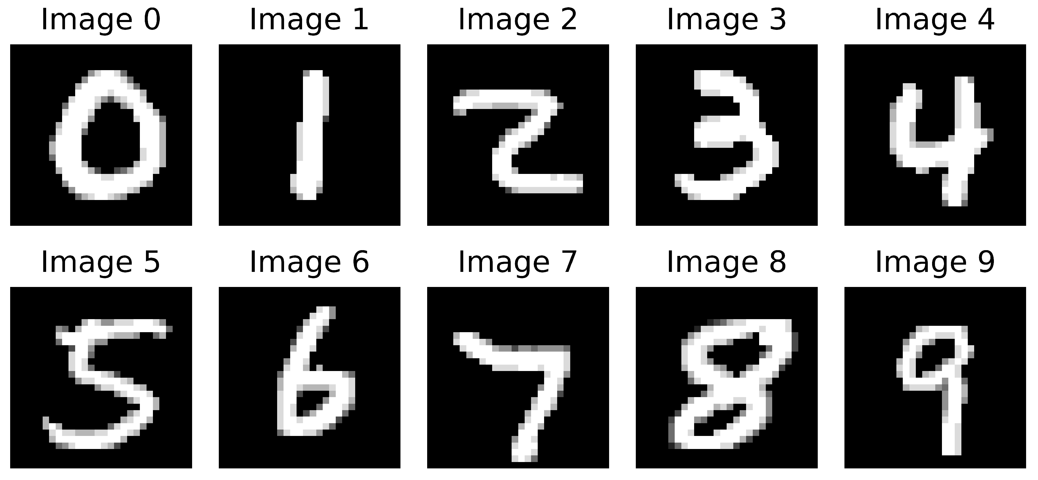
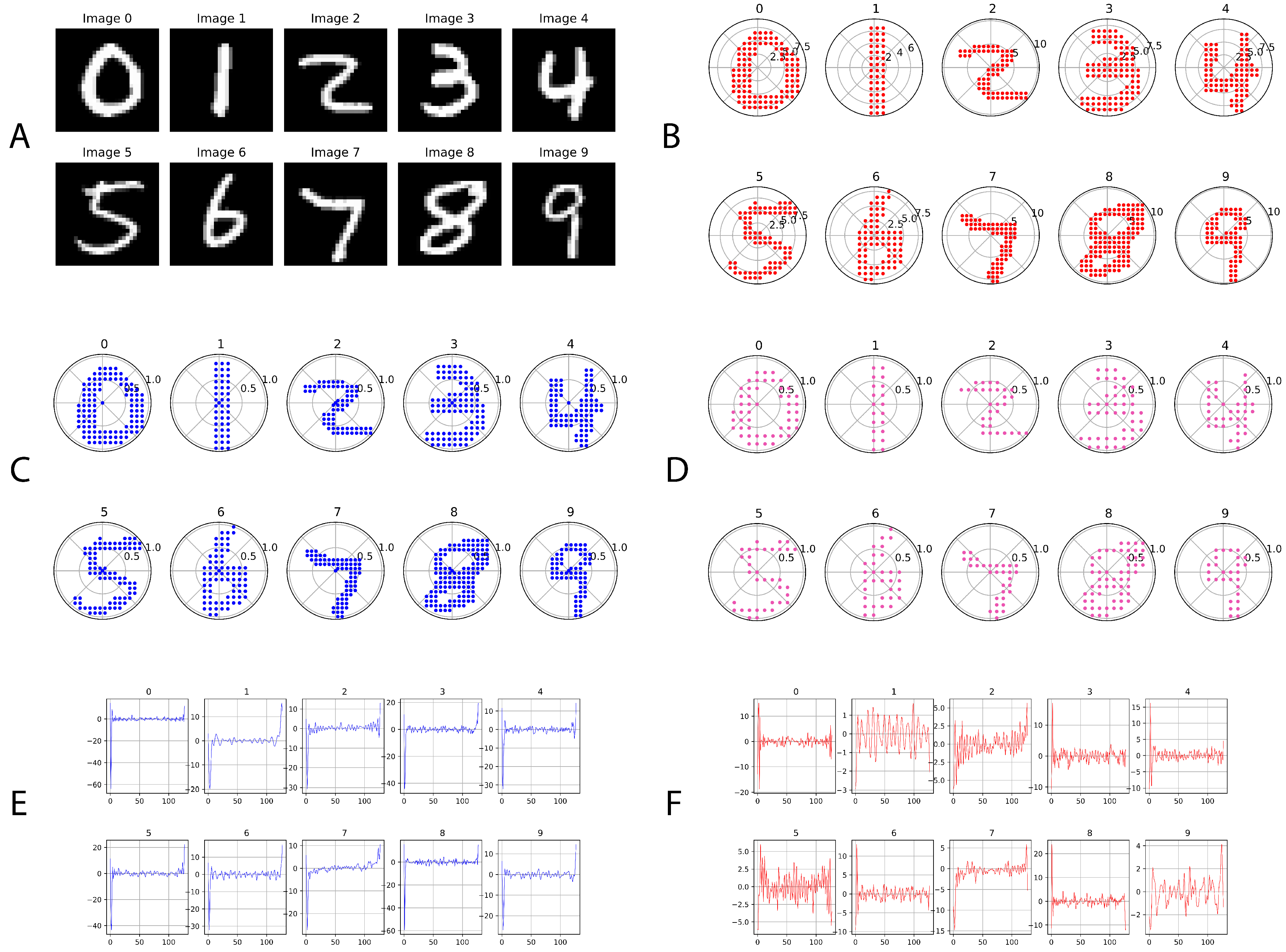
In the present study, the MNIST database of handwritten digit images was employed. Recognized as a benchmark dataset for neural network modeling and computer vision, the MNIST dataset consists of handwritten digits from 0 to 9. This dataset is commonly utilized for the training and assessment of classification algorithms. As depicted in Figure 2(A), the dataset offers representative samples of each numeral from 0 through 9. It has 60,000 training and 10,000 testing samples. It is noteworthy that the pixel values within these images span from 0 to 255, indicating the grayscale intensity.

In our study, we explored a methodology from a published paper[8] that transitions MNIST images from the traditional cartesian coordinate system (x and y) to the polar coordinate system, defined by magnitude (

ρ

) and angle (

θ

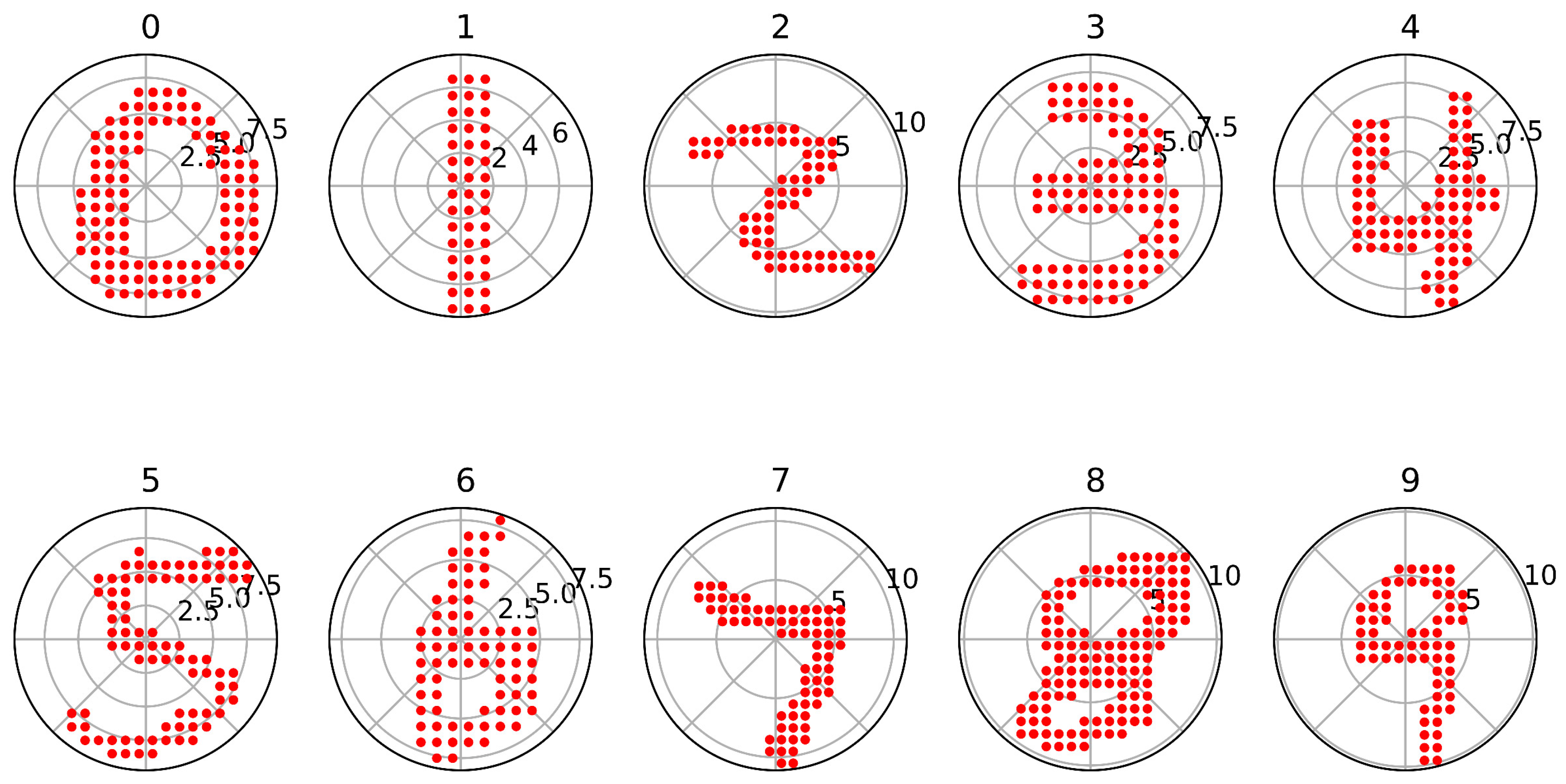
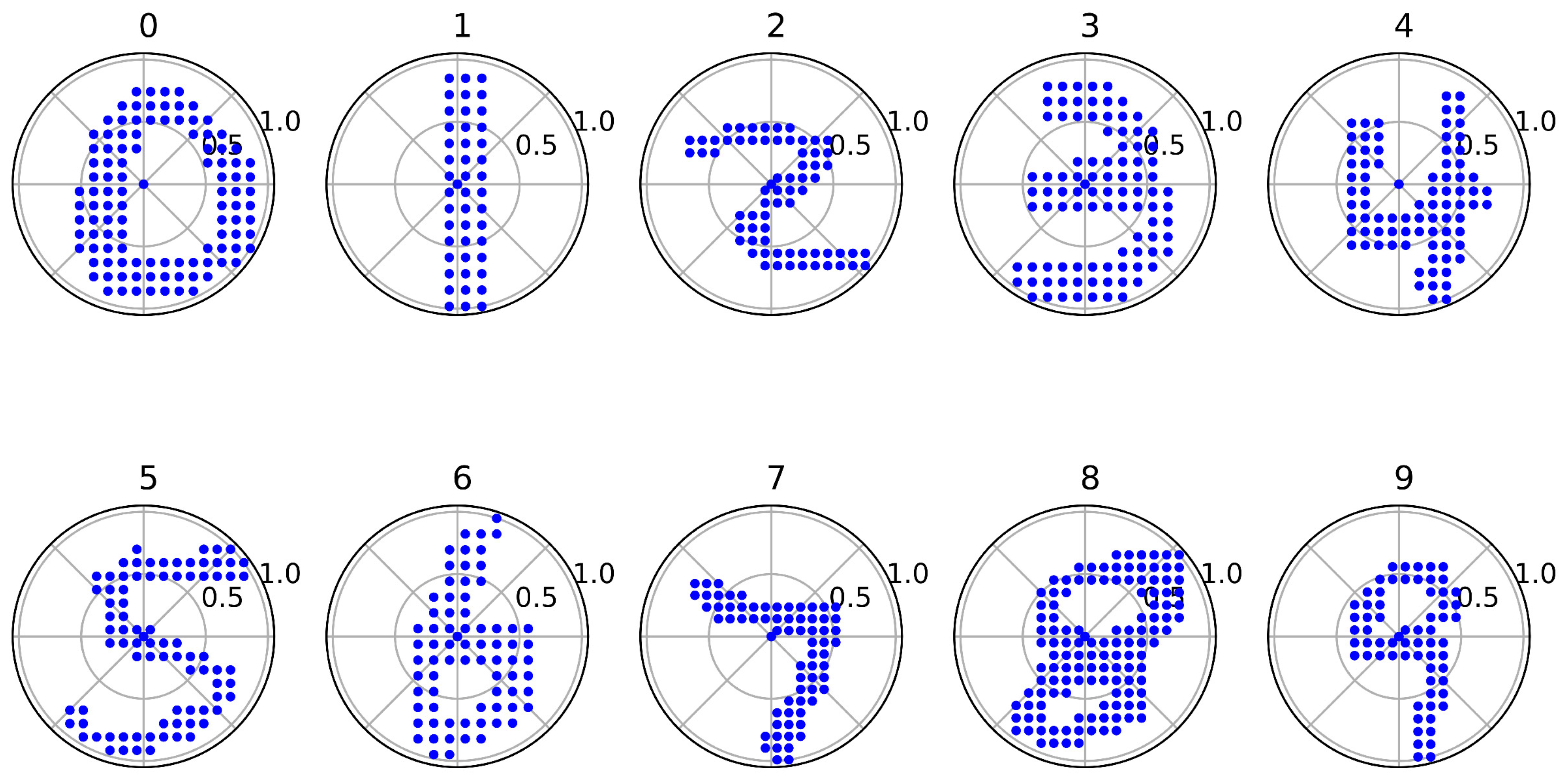
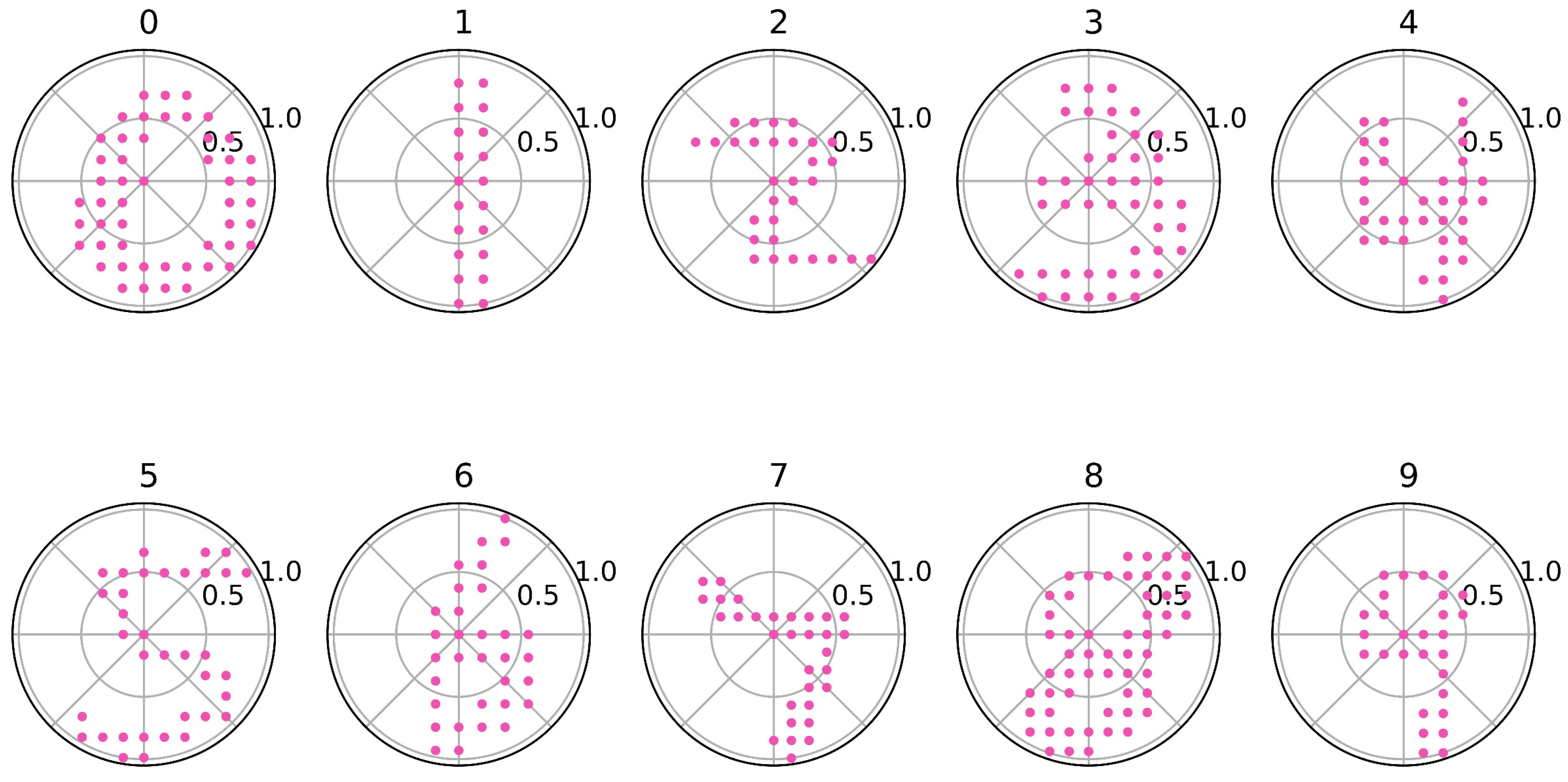
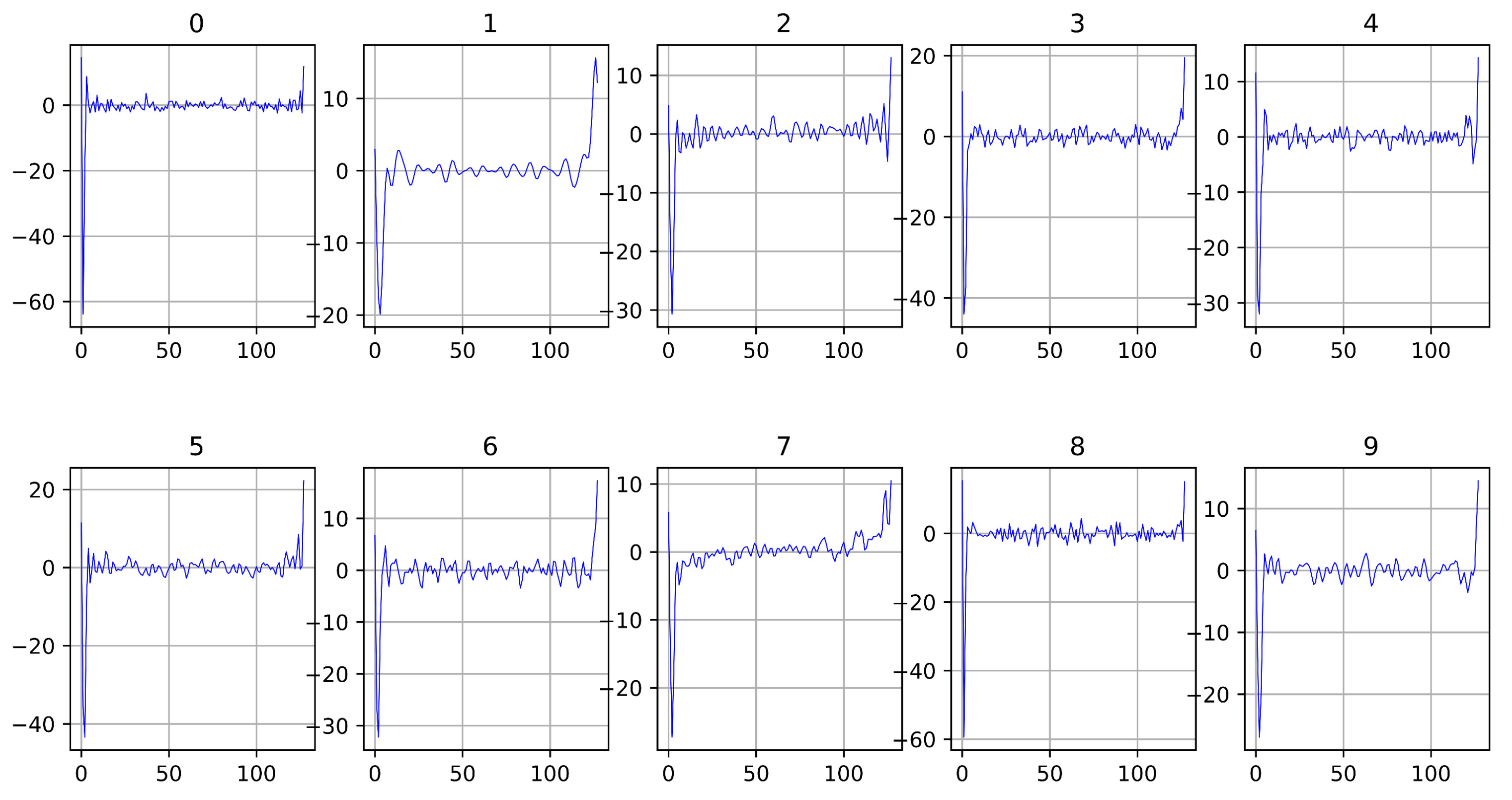
), using complex number representation. This technique effectively captures the spatial characteristics of pixel locations and their relationships during serialization. Figure 2 shows the a sample of 0-9 original MNIST digits, polar-coordinate representation, and serialized view after Discrete Fourier Transformation.

To convert from Cartesian to polar coordinates, a series of steps is undertaken, including a Logarithmic transformation, contour highlighting, down-sampling, and the actual Cartesian to Polar coordinate transformation. The resulting polar-represented MNIST digits can be seen in Figure 2(B). Following this, Zero-Padding and Decimation techniques are employed to select a specific number of data points. Figure 2(C) displays the polar-represented images with 128 data points, while Figure 2(D) illustrates the images with 64 data points. Finally, the polar-represented images undergo serialization through Discrete Fourier Transform (DFT), which captures both the amplitude and phase of specific frequency components within the original sequence, as depicted in Figure 2(E and F). The detailed process for these steps is discussed in Appendix A.

3. Complex-valued Neural Network (CVNN) implementation

CVNNs represent a specialized class of neural networks that operate on complex numbers, encompassing both real and imaginary components [23]. While conventional neural networks primarily deal with real-valued data, CVNNs have gained prominence in applications where data inherently exhibits both magnitude and phase information, especially those involving signals, waves, or data with phase information.

In the context of this study, the relevance of CVNNs stems from their intrinsic capability to effectively process complex-valued data. The research is focused on the preprocessed MNIST dataset, which undergoes a transformation from Cartesian to polar coordinates, followed by serialization using the discrete Fourier transform (DFT). This transformation equips the dataset with complex numbers, enabling a more compact representation while retaining critical phase information, which is essential for character recognition tasks [24].

3.1. Complex Numbers in Neural Networks

A complex number is represented as

z = a + b i

where a is the real part, b is the imaginary part, and i is the imaginary unit with the property

i^{2} = - 1

When dealing with CVNNs, both the weights and the activations can be complex numbers. This means that when computing the weighted sum in a neuron, both the real and imaginary parts of the weights and inputs need to be considered.

3.2. Architectural Choices for CVNN:

1. Layers: Just like real-valued neural networks, CVNNs can have input layers, hidden layers, and output layers. The number of layers and the number of neurons in each layer will depend on the specific problem and the complexity of the data.

a. Input Layer: The input layer of the CVNN corresponds to the serialized complex-valued representation of MNIST images in this work. For each input data point, the CVNN processes both real and imaginary components as a single complex number, thus requiring an input layer with a size corresponding to the dimensionality of the complex input.

b. Hidden Layers: The hidden layers of the CVNN typically consist of multiple complex-valued neurons. The number of hidden layers and the number of neurons in each layer are architectural hyperparameters optimized during the network’s training process.

2. Neurons: In CVNNs, each neuron can accept complex-valued inputs and produce a complex-valued output. The computation within a neuron involves both the real and imaginary parts of the weights and inputs. The weighted sum for a neuron is given by:

z = \sum_{j} w_{j} x_{j} + b

(1)

where

w_{j}

and

x_{j}

are complex numbers, and b is a complex bias term. The weighted sum is then passed through a complex activation function.

3. Activation Functions: Activation functions introduce non-linearity into the network, enabling it to model complex relationships.

CReLU: The complex rectified linear unit (CReLU) [25] activation function extends the real-valued ReLU to complex numbers while preserving the phase information. It is defined as:

$f (z) = max (0, Re (z)) + i max (0, Im (z))$

(2)

4. Output Layer:

The output layer of the CVNN is responsible for producing predictions. For classification tasks, the softmax function can be extended to handle complex numbers, ensuring the outputs can be interpreted as probabilities. The complex-valued softmax [25] is given by:

σ {(z)}_{j} = \frac{e^{z_{j}}}{\sum_{k = 1}^{K} e^{z_{k}}}

(3)

where K is the number of classes.

3.3. CVNN Model

1. Forward Pass: During the forward pass, input data propagates through the network’s layers, undergoing linear transformations and activations. The result of the forward pass is the network’s prediction. The weighted sum of its inputs is calculated by 1.

2. Backward Pass: The backward pass is where gradients are computed with respect to the network’s parameters. Gradients are essential for optimizing the model during training. The backpropagation algorithm’s primary goal is to compute the gradient of the loss function with respect to the weights. With complex numbers, this involves the Wirtinger derivatives [26].

Given a loss function L that is a function of a complex output z, the gradient with respect to a complex weight w is:

\frac{\partial L}{\partial w} = \frac{\partial L}{\partial z} \frac{\partial z}{\partial w^{*}} + \frac{\partial L}{\partial z^{*}} \frac{\partial z}{\partial w}

(4)

Here,

\frac{\partial z}{\partial w^{*}}

is the conjugate of the input associated with the weight w.

3. Update Rule: The update rule specifies how the network’s parameters are adjusted based on the computed gradients. We use optimization algorithms like Adam and Stochastic Gradient Descent (SGD) to update weights during training.

Gradient Descent [27]

Given a function $f (w)$ , where $w$ is a vector of parameters, the goal of gradient descent is to find the value of $w$ that minimizes f.

The update rule for gradient descent is:

$w_{new} = w_{old} - α \nabla f (w_{old})$

(5)

Where:

−

$α$ is the learning rate.

−

$\nabla f$ is the gradient of f with respect to $w$ .
Complex Gradient Descent [28]

When dealing with functions of complex variables, the gradient descent update rule can be extended to handle complex numbers. Let’s say our function is $f (z)$ , where z is a complex variable. The gradient in the complex domain is often referred to as the Wirtinger derivative.

The Wirtinger calculus provides us with two partial derivatives:

$\frac{\partial}{\partial z} and \frac{\partial}{\partial z^{*}}$

(6)

Where $z^{*}$ is the complex conjugate of z.

The gradient of f with respect to z and $z^{*}$ is given by:

$\nabla f = (\frac{\partial f}{\partial z}, \frac{\partial f}{\partial z^{*}})$

(7)

The update rule for complex gradient descent can then be written as:

$z_{new} = z_{old} - α \frac{\partial f}{\partial z^{*}}$

(8)

Note: The choice of using $\frac{\partial f}{\partial z^{*}}$ in the update rule is a convention. Depending on the specific problem or context, the other derivative $\frac{\partial f}{\partial z}$ might be used.

4. Weight Initialization: The weights in CVNNs are complex. Therefore, both the real and imaginary parts of the weights need to be initialized.

5. Complex Batch Normalization [25]

Batch normalization is a technique to improve the training of deep neural networks by normalizing the activations of each layer. For CVNNs, this normalization should be applied separately to the real and imaginary parts. Given a complex activation z, the batch-normalized output

\hat{z}

is:

\hat{z} = \frac{z - μ}{\sqrt{σ^{2} + ϵ}}

(9)

Where:

$μ$ is the mean of the activations (computed separately for real and imaginary parts).
$σ^{2}$ is the variance (also computed separately).
$ϵ$ is a small constant to prevent division by zero.

3.4. Training Procedure and Hyperparameters

We have developed a CVNN using the cvnn library, which is open-source and accessible on GitHub [https://github.com/NEGU93/cvnn]. Detailed documentation can be found on Read the Docs [https://complex-valued-neural-networks.readthedocs.io/en/latest/index.html]. This library is distributed under the MIT License, promoting flexibility and ease of use for the community.

Our CVNN architecture is designed as a feedforward model, constructed using TensorFlow’s renowned Sequential API. The network structure consists of an initial input layer, followed by two dense layers, carefully crafted to efficiently process and manage complex-valued data.

Table 1. The programming language and libraries used for build- ing the model are as follows

Item	Description
Language	Python
Main Libraries	TensorFlow and Keras
Custom Library	cvnn, which provides specialized layers and functions for complex-valued neural networks.

3.4.1. The parameters for the feedforward model are configured as follows:

The model begins with a ’ComplexInput’ layer with an input shape of 128 or 64.
Subsequently, a "ComplexDense" layer is added with a varying number of neurons, depending on the specific model. The "crelu" [equation 2] activation function is chosen, and the layer is initialized with the ’ComplexGlorotUniform’ initializer.
The final layer in our model is another "ComplexDense" layer with 10 neurons for the classification of ten different MNIST handwritten digits. It utilizes the "cart_softmax" activation function and is initialized with the ’ComplexGlorotUniform’ initializer.

3.4.2. The training parameters for the CVNN are configured as follows:

Optimizer: We have used the ’Adam’ optimizer, a well-known optimization algorithm that adapts the learning rate during training.
Loss Function: Our model employs the ’ComplexAverageCrossEntropy’ loss function, which applies Categorical Cross Entropy to both the real and imaginary parts separately and then averages the results.
Metrics: Model performance is evaluated using the ’ComplexCategoricalAccuracy’ metric, which measures how often predictions match one-hot labels.
Training: The model is trained using the ’fit’ method with a batch size of 32 and a specified number of epochs (in our case, 50). Both training data (’train_images’ and ’train_labels’) and validation data (’val_images’ and ’val_labels’) are provided to this method.
Learning Rate: Our implementation does not specify any learning rate schedules, so the learning rate defaults to the value set by the ’Adam’ optimizer, which is ’0.001’.

3.5. Experimental Setup

In this section, we outline the comprehensive experimental setup for our study, conducted on Google Colab, utilizing the Ubuntu 22.04.2 LTS environment with abundant system resources. We detail the hardware and software configurations, as well as the dataset and model variations considered.

3.5.1. Hardware and Software Environment

Our experiments were conducted on Google Colab, specifically version 1.0.0, which offers a robust cloud-based environment for machine learning tasks. The underlying specifications of the environment are as follows:

Table 2. Hardware and Software Environment Details

Hardware and Software Environment
Operating System	Ubuntu 22.04.2 LTS
System RAM	51.0 GB
CPU	Intel(R) Xeon(R) CPU @ 2.00GHz
Python Version	3.10.12
TensorFlow Version	TensorFlow 2.13.0

3.5.2. Dataset and Model Variations

Our research investigates the impact of varying the number of data points for input within the context of polar-represented serialized MNIST digit datasets. In order to conduct a comprehensive analysis of the performance of our models, we have developed two independent models with varying input configurations:

Table 3. Model Configurations

Model 1: 128 Data Points	Model 2: 64 Data Points
Input Layer Neurons: 128	Input Layer Neurons: 64
Hidden Layers Neurons: 10, 15, 20, 25, 30, 50, 100	Hidden Layers Neurons: 10, 15, 20, 25, 30, 50, 100
Output Layer Neurons: 10	Output Layer Neurons: 10
Batch Size = 32	Batch Size = 32
Number of Epoch: 50	Number of Epoch: 50

The deliberate manipulation of the quantity of data points enables us to thoroughly assess the effectiveness of our models across various input configurations.

3.5.3. Dataset Details

The dataset utilized in this study consists of serialized MNIST digit pictures rendered in polar coordinates. This representation offers the benefit of reducing the number of data points required for input. The dataset encompasses a range of key statistical measures, which are as follows:

Table 4. Dataset Details

Dataset Details
Training Samples	60,000
Testing Samples	10,000
Validation Split	0.02% of the training data was set aside for validation

The dataset at our disposal is highly suitable for evaluating the efficacy of our models, hence facilitating the derivation of significant comparisons and insights.

In brief, the experimental configuration for our study is established within a reliable Google Colab environment that offers substantial computational capabilities. In this study, we examine the influence of various input configurations on the performance of a model. Our analysis is based on a dataset consisting of serialized MNIST digit pictures stored in polar form. The purpose of this configuration is to enable thorough examinations and offer significant observations regarding the performance of our models.

4. Results and Performance Evaluation

This section provides an overview of the experimental results and performance evaluation of the CVNNs when trained on the preprocessed MNIST dataset. Our team offers complete insights into our model’s behaviour through the provision of thorough visualizations, encompassing accuracy trends, training curves, and loss plots.

In the present study, we utilize two separate models of CVNNs. The initial model, referred to as CVNN_Polar_128, is specifically designed to handle a dataset that is serialized in the Polar representation and consists of 128 datapoints. On the other hand, the second model is designed to accommodate a comparable dataset, albeit with a diminished count of 64 datapoints, and is appropriately denoted as CVNN_Polar_64.

4.1. Accuracy Metrics

To assess the model’s performance comprehensively, we analyze the accuracy trends for both of the models with the Serialized Polar-represented testing datasets.

4.1.1. Graph Interpretation

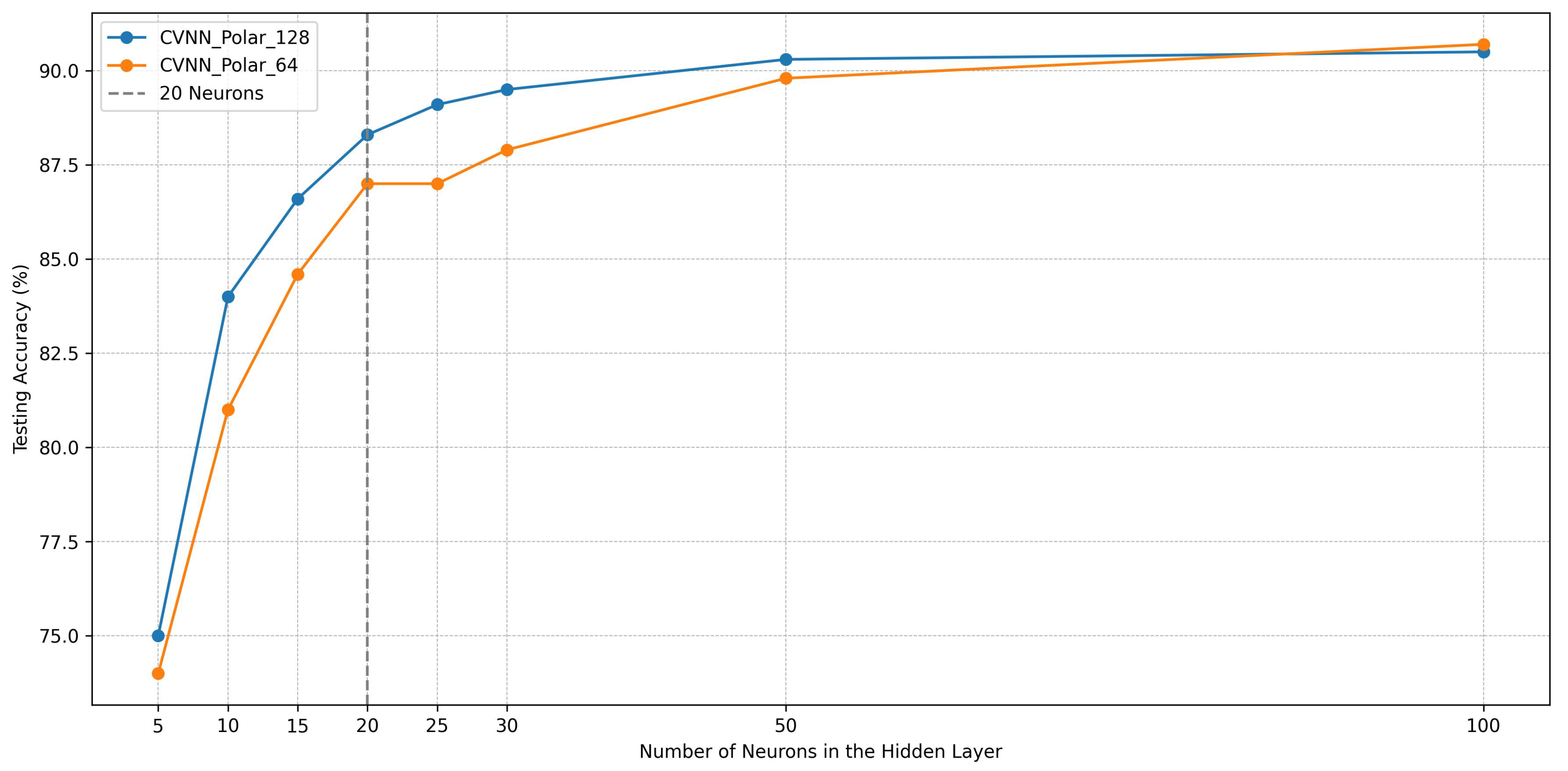
The graph in the Figure 3 visualizes the testing accuracy of two complex-valued neural network models, CVNN_Polar_128 and CVNN_Polar_64, against the number of neurons in their hidden layers. The horizontal axis delineates the neuron count, ranging from 5 to 100, while the vertical axis marks the achieved testing accuracy, expressed as a percentage. A vertical dotted line at "20 Neurons" highlights the chosen neuron count, offering a visual cue for the selection. Both models demonstrate a general upward trend, suggesting that increasing the neuron count positively impacts the accuracy, up to a certain threshold.

4.1.2. Performance Insights

CVNN_Polar_128 consistently outperforms CVNN_Polar_64 for neuron counts up to 20. Beyond this, the performance difference narrows, with CVNN_Polar_64 eventually achieving slightly higher accuracy at 100 neurons.
The most significant rise in accuracy for both models is observed between 5 to 20 neurons, after which the gains in accuracy start to plateau.

4.1.3. Justification for Selection of 20 Neurons

From an optimization standpoint, selecting 20 neurons for the hidden layer of both models appears judicious for several reasons:

Balanced Complexity and Performance: At 20 neurons, both models achieve a substantial increase in accuracy compared to lower neuron counts, without the added computational overhead of higher counts. This makes the models efficient without compromising on performance.
Diminishing Returns: While further increments in neuron count do lead to accuracy improvements, the gains become marginal. For instance, the leap from 20 to 100 neurons results in an increase of just over 2% for both models, which may not justify the associated computational cost and potential overfitting risks.
Generalization: A model with fewer neurons is less prone to overfitting. With 20 neurons, CVNN_Polar_128 achieves an accuracy of 88.3%, and CVNN_Polar_64 attains 87%. These figures highlight efficient model architectures given the neuron count.
Computational Efficiency: Neural networks with fewer neurons train faster and require less memory. From a practical standpoint, especially in real-time applications or scenarios with limited computational resources, a leaner model is advantageous.

In the conducted experiments, two CVNN models were trained on the preprocessed MNIST dataset: CVNN_Polar_128 with 128 datapoints and CVNN_Polar_64 with 64 datapoints. Performance evaluations, visualized through accuracy trends, training curves, and loss plots, details provided in Appendix revealed that CVNN_Polar_128 generally outperformed CVNN_Polar_64, especially with up to 20 neurons in the hidden layer. Both models exhibited an optimal balance of complexity and performance at this neuron count, while further increments showed diminishing returns. Specifically, the CVNN_Polar_128 model achieved an overall accuracy of 88% on a 10,000-sample test dataset of the MNIST.

4.2. Comparison with Real-Valued Neural Networks

In this section, we compare the performance of CVNNs with RVNNs in handling complex data, specifically the polar-transformed MNIST digit dataset. We delve into accuracy metrics between these two types of networks, shedding light on the advantages of employing CVNNs for complex data.

4.2.1. Objective & Hypothesis

The central proposition behind adopting the polar representation was to minimize the datapoint requirements for a neural network. By reducing the number of neurons in the input layer, we anticipated not only a decrease in computational demands but also a faster training and testing process, leading to energy savings. A key hypothesis was that CVNNs, given their ability to process magnitude and phase information directly, would have an edge over traditional RVNNs when presented with complex data.

4.2.2. Models Overview:

RVNN_Raw_MNIST: A real-valued neural network that operates directly on the original MNIST dataset without any preprocessing. This model serves as a benchmark, providing a standard to which other models can be compared.
CVNN_Polar_128 & CVNN_Polar_64: Complex-valued neural network models that ingest the serialized polar-transformed MNIST dataset. The numerals ’128’ and ’64’ denote the number of datapoints (or complex numbers) each model processes.
RVNN_Polar_128 & RVNN_Polar_64: Real-valued adaptations designed to handle the polar-transformed dataset. To accommodate the complex nature of the data, these models separate and concatenate the real and imaginary parts, effectively doubling their input neuron requirements.

4.2.3. Processing Complex Data in Real-Valued Networks

By segregating the real and imaginary components of the serialized polar-transformed MNIST dataset and then concatenating them, the models were furnished with doubled input fields. This ensured that the entirety of the complex data was captured, albeit in a format palatable to real-valued networks. For instance, the RVNN_Polar_128 model, designed for 128 complex datapoints, required 256 neurons in its input layer to accommodate both the real and imaginary parts.

When comparing the RVNN and CVNN models, both were configured with an identical number of hidden layer neurons, set at 20 for this analysis.

Additionally, other parameters, including the number of output layer neurons, batch size, and epochs, were kept uniform across both models for a consistent evaluation.

4.2.4. Performance Insights

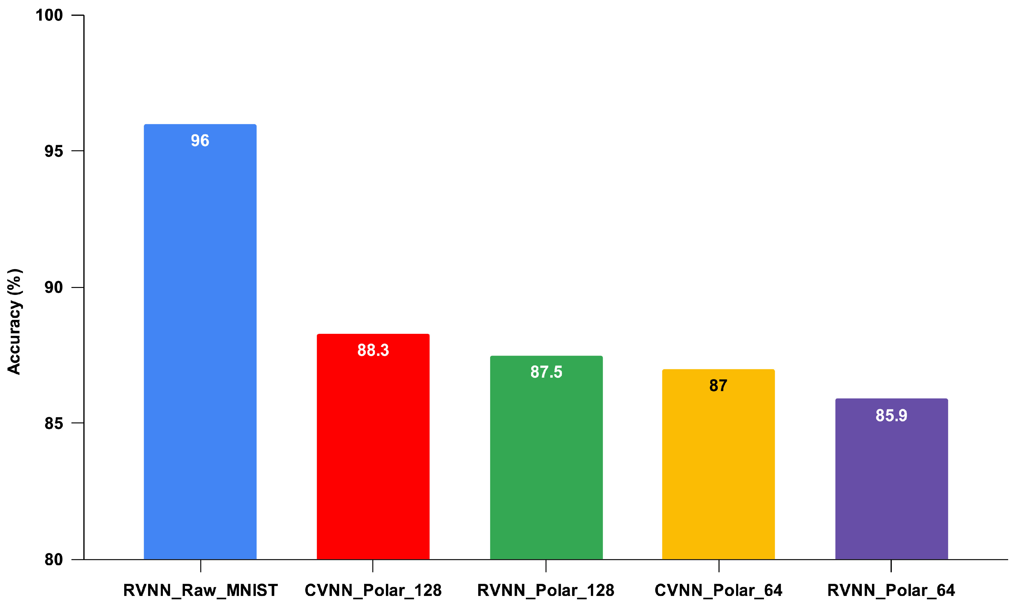
Benchmark Performance: While the RVNN model operating on the original MNIST dataset set a high standard with an accuracy of 96%, our focus was primarily on the performance gains achieved through polar transformation.
Complex-Valued vs. Real-Valued on Polar Data: As hypothesized, the CVNN_Polar_128 model, attaining an accuracy of 88.3%, outperformed its RVNN counterpart, RVNN_Polar_128, which secured 87.5%, showed in Figure 4. This 0.8% differential underscores the inherent advantage of CVNNs when processing polar-transformed data. The separation of real and imaginary components in RVNNs, while necessary, may lead to the omission of valuable interplay between these components, a nuance that CVNNs naturally capture.
Data Efficiency through Polar Transformation: The polar-transformed models, even with reduced datapoints, achieved commendable accuracies. The slight performance trade-offs were balanced by the benefits of reduced computational requirements and energy consumption.

4.2.5. Testing accuracy cross various neuron counts

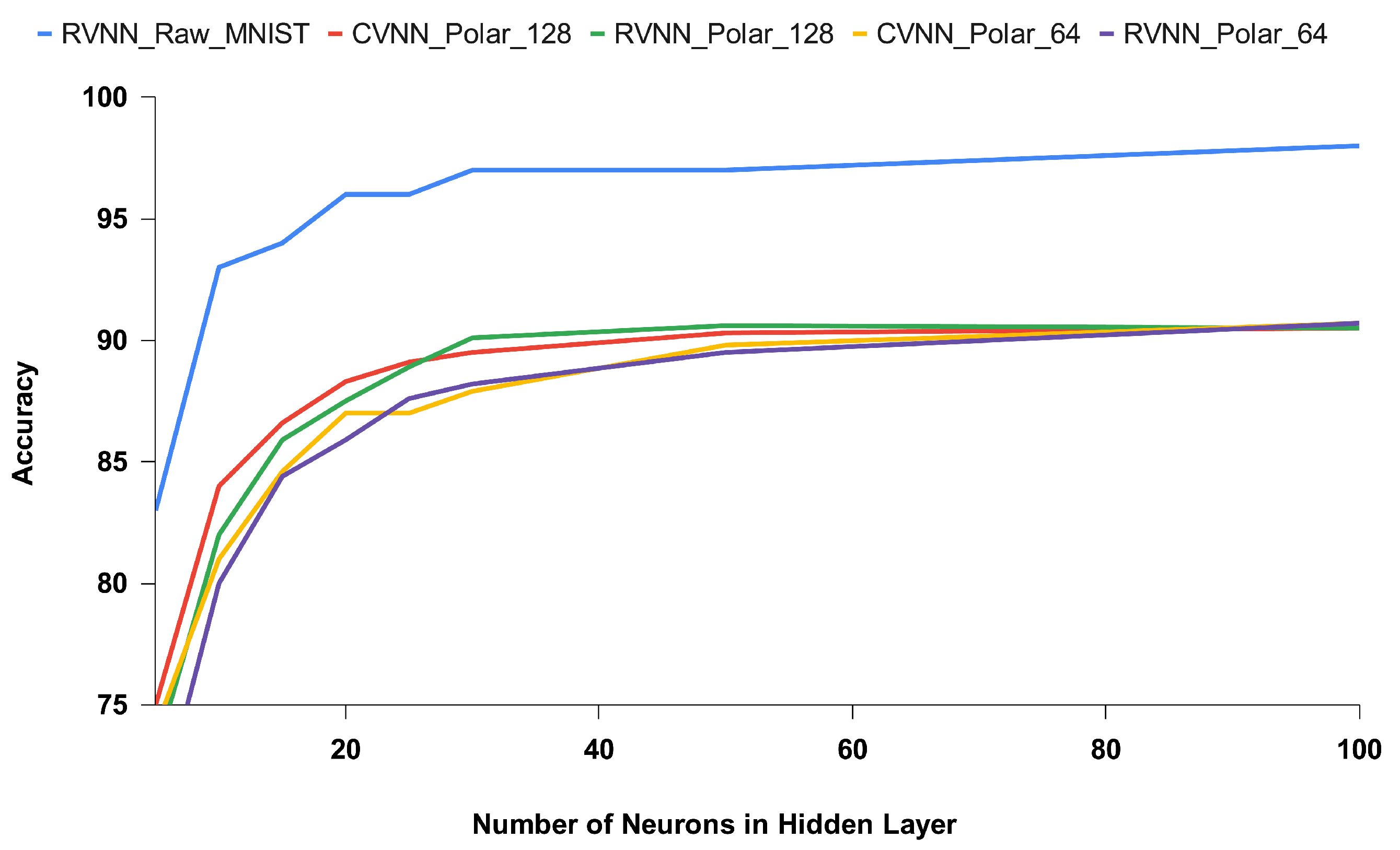
The graph in Figure 5 delineates the testing accuracies of various neural network models based on different neuron counts in the hidden layer. Notably, the "RVNN_Raw_MNIST" model, processing the original dataset, exhibits superior performance, reaching 98% accuracy with 100 neurons. In contrast, models working with polar-transformed data display a consistent trend: CVNNs initially outperform their RVNNs, especially at lower neuron counts. However, as neuron counts rise, the performance disparity narrows, with RVNNs nearly matching CVNNs, especially at 100 neurons. This underscores the RVNNs’ adaptability and the inherent advantage of CVNNs with complex data, while also highlighting the diminishing returns of increasing neuron count

4.2.6. Comparison with Contemporary Research

Jose Agustin Barrachina, in his implementation of the CVNN model [29], conducted MNIST handwritten digits classification. He transformed the original MNIST dataset from its real-valued version to a complex-valued version using TensorFlow’s tf.cast function and tf.complex64 data type. This conversion resulted in each pixel of the image comprising both real and imaginary components. Following testing, he achieved an impressive 99% accuracy for the MNIST dataset. In our comparison table, we refer to Jose Agustin Barrachina’s model as CVNN_JAB.

Table 5. Accuracy Comparison with contemporary research

Model	Accuracy
CVNN_Polar_128	88.3%
CVNN_JAB	99%

While his model achieved higher accuracy, it came at the cost of increased computational complexity. This was due to the inclusion of all 784 data points for each MNIST image. In contrast, our model only utilized 128 data points, resulting in reduced computational demands. This makes it a more efficient choice for hardware accelerator implementation in resource and energy-constrained environments.

According to the PapersWithCode.com website, as of today, the highest accuracy achieved in MNIST classification is 99.83% by Byerly A et al. [30].

4.3. Conclusion

The research affirms the efficacy of polar-transformed datasets in optimizing neural network performance, both in terms of accuracy and computational efficiency. Notably, CVNNs, with their intrinsic capability to handle complex data, demonstrated superiority over RVNNs in this context. These findings pave the way for further exploration into the synergies between data transformation techniques and neural network architectures, potentially leading to even more efficient and eco-friendly machine learning models.

5. FPGA Implementation of CVNNs

In this section, we transition from the theoretical aspects discussed in the previous sections, which focused on the polar representation of 2D images, serialization techniques, and their application to neural networks (CVNN and RVNN) for MNIST handwritten digit classification. Here, our focus shifts to the hardware implementation of these neural network’s inference models, with a specific emphasis on CVNNs, using FPGA.

FPGAs are chosen as the hardware platform for several compelling reasons. These include their inherent capabilities for massive parallelism, reconfigurability, and power efficiency. In contrast to CPU-based systems, which operate sequentially, and GPUs, which lack reconfigurability, FPGAs offer a unique combination of performance, adaptability, and energy efficiency, making them an ideal choice for accelerating complex neural network computations.

The evolution of digital systems design has been marked by several significant milestones, with the inception of FPGA being a prominent one. Unlike ASIC, which are permanently dedicated to a specific function after manufacturing, FPGAs are distinct due to their reprogrammable nature, allowing them to be tailored for multiple applications post-production [31]. This feature offers a level of versatility that’s unparalleled in the realm of digital design.

5.1. FPGA’s Role in Neural Network Acceleration

The renaissance of neural networks and deep learning, driven by the surge in data and computational power, has ignited the need for specialized hardware accelerators. FPGAs, with their ability to parallelize operations, are emerging as a frontrunner in this domain [32]. Neural networks often involve matrix multiplications, convolutions, and other operations that can be parallelized. The inherent architecture of FPGAs, with its myriad of reconfigurable logic blocks, can be optimized to handle such operations simultaneously, offering a significant speedup compared to sequential processors. Moreover, the dynamism of the field of artificial intelligence means that algorithms and models are continually evolving. FPGAs, with their reprogrammable nature, ensure that as newer models or techniques emerge, the hardware can be reconfigured to adapt, ensuring longevity and relevance in deployment.

5.2. Complex-Valued Neural Network Inference Model

In the previous sections, we delved into the intricacies of forward and backward propagation within the CVNNs. As we transition into this section, our primary focus is on offering a succinct recapitulation of forward propagation. This is imperative for a holistic understanding of how we have implemented the CVNN inference model on FPGA.

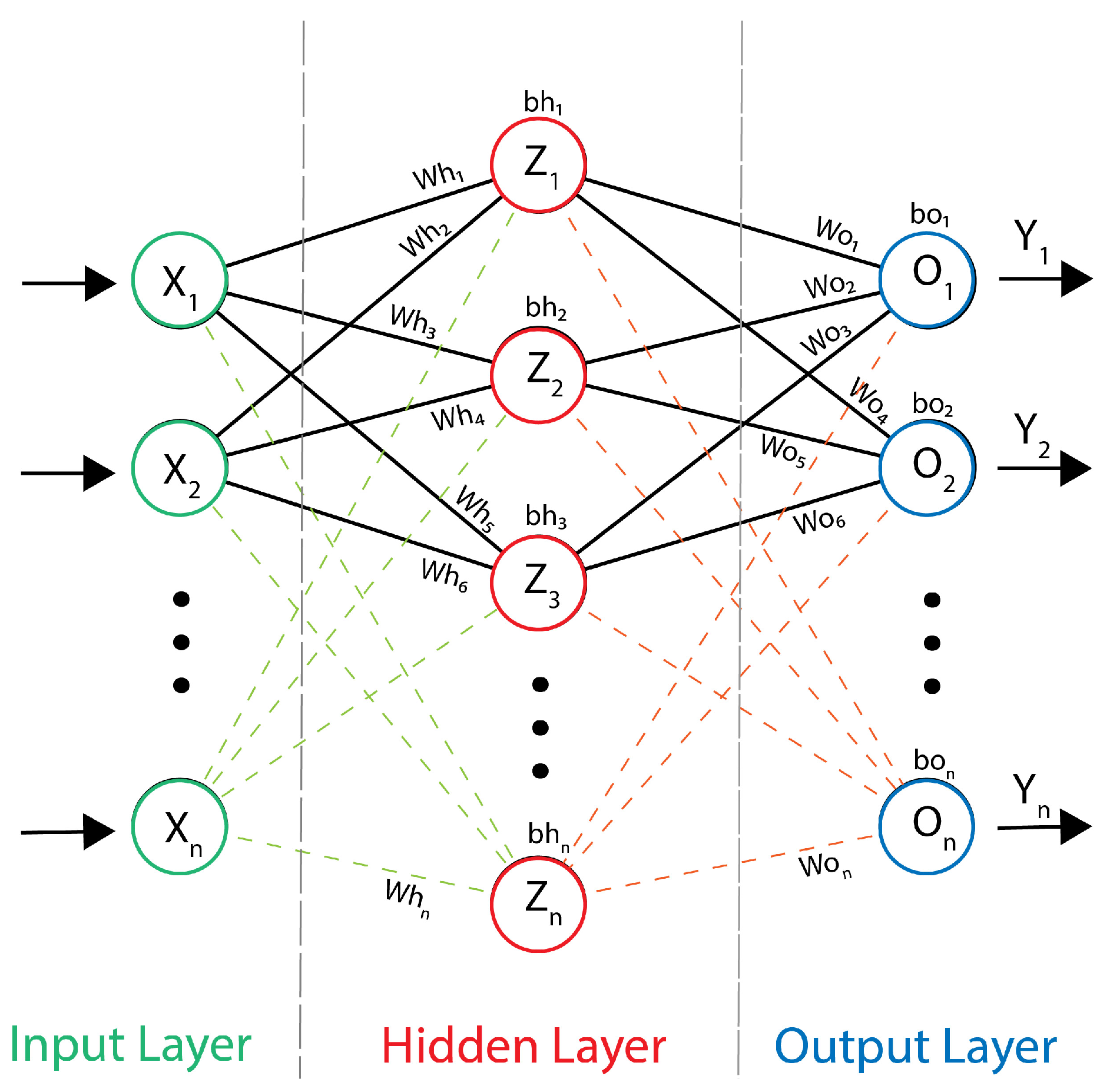
Our implementation of the CVNN inference model leverages the weights and biases from a pre-trained model. For a visual representation of our CVNN model’s architecture, one can refer to Figure 6. It’s pivotal to note that all the parameters, including input X, weight W, bias b and output Y, are complex-valued in this architecture.

Complex numbers in our context are typically depicted as

a + b i

, where a signifies the real part, b stands for the imaginary part, and i is the imaginary unit.

To elucidate further, let’s dissect the model’s operations:

1.: Weighted Sum in Hidden Layer: The first step in our forward propagation is the computation of the weighted sum for each neuron in the hidden layer. This is achieved by linearly combining the complex-valued inputs with their respective weights, adding the complex-valued biases subsequently. For instance, the weighted sum $Z_{1}$ for the first neuron in the hidden layer can be represented as:

$Z_{1} = X_{1} \times W h_{1} + X_{2} \times W h_{2} + \dots + X_{n} \times W h_{n} + b h_{1}$

(10)

Where, X refers to complex inputs, $W h$ refers to the complex weights in the hidden layer, and $b h$ denotes the complex biases in the hidden layer.
2.: Activation in Hidden Layer: Following the computation of the weighted sum, we introduce non-linearity through the Complex ReLU (CReLU) activation function. This function, applied to each neuron’s weighted sum, separates the real and imaginary components. It then rectifies negative values from both parts. For the first neuron, the activation is:

$H_{1} = CReLU (Z_{1}) = max (0, Real (Z_{1})) + i \times max (0, Imag (Z_{1}))$

(11)

Where, H is the output of a hidden layer neuron after activation.
3.: Weighted Sum in Output Layer: The outputs from the hidden layer are then used to compute the weighted sum for each neuron in the output layer. This involves multiplying each output from the hidden layer by the respective weights of the output neurons and adding the corresponding biases.

$O_{1} = H_{1} \times W o_{1} + H_{2} \times W o_{2} + \dots + H_{n} \times W o_{n} + b o_{1}$

(12)

Where, $W o$ are the weights in the output layer, $b o$ are the biases in the output layer, and O is the weighted-sum of a neuron in the output layer.
4.: Activation in Output Layer: Finally, the CReLU activation function is once again applied to the weighted sums from the output layer to yield the final complex-valued outputs of the model. Using the first output neuron as an example:

$Y_{1} = CReLU (O_{1}) = max (0, Real (O_{1})) + i \times max (0, Imag (O_{1}))$

(13)

In the original CVNN model, the softmax activation function was employed for the output layer, providing a probabilistic interpretation of the model’s predictions. However, when transitioning to FPGA implementation, it’s imperative to strike a balance between computational accuracy and hardware efficiency. Given this consideration, we opted for the CReLU activation function in our project. This choice not only streamlines the FPGA implementation but also ensures a robust performance, while simplifying the overall computational complexity.

In our pursuit to draw a comprehensive comparison with the CVNN model, we implemented a RVNN inference model on FPGA. The underpinnings of this implementation draw many parallels to the CVNN model.

For the RVNN, we took a strategic approach by separating the complex-valued inputs into their real and imaginary components. These separated components were then treated as independent real-valued inputs. Consistent with the RVNN paradigm, the weights, biases, and activation functions were all real-valued. Specifically, the ReLU activation function was employed for the RVNN, described by the equation:

H_{n} = ReLU (Z_{n}) = max (0, Z_{n})

(14)

This function effectively nullifies negative values, allowing only positive activations to propagate through the network. By juxtaposing the CVNN and RVNN models, we aim to provide a holistic understanding of their respective performances and intricacies on FPGA platforms.

5.3. FPGA Implementation of Inference Model

In our previous discussions, we thoroughly examined the mathematical foundations inherent to the inference models of neural networks that were central to our research. Transitioning from theory to application, the linchpin of the FPGA implementation of these models is the precise crafting of VHDL modules that correspond to each step and mathematical equation. At the heart of the architectures of both the CVNNs and RVNNs lie several core modules: adders, multipliers, and the specific activation functions - Complex Linear Rectified Unit (CReLU) and the traditional Rectified Linear Unit (ReLU).

For this FPGA-centric endeavor, we predominantly utilized Vivado v2021.1 64-bit for design and synthesis, combined with VHDL for hardware description and programming.

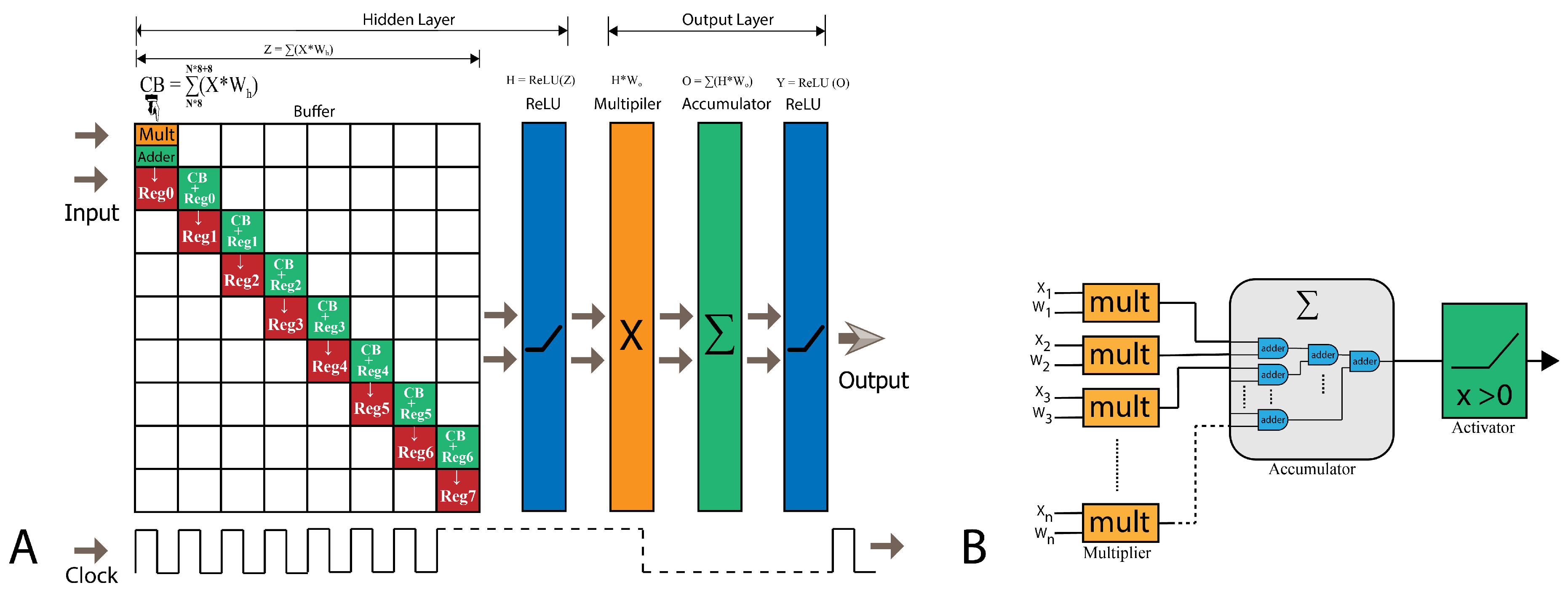
The accompanying Figure 7(B) offers a schematic representation of a singular neuron’s FPGA realization.

5.3.1. Adder

Real-valued adder:

The adder module for real numbers in a digital FPGA environment is implemented using fixed-point arithmetic. In fixed-point representation, every number is represented as an integer and a fractional part. Mathematically, given two fixed-point numbers A and B, the summation S is given by:

S = A + B

(15)

Complex-valued adder: Complex numbers consist of real and imaginary components. Thus, for two complex numbers

C_{1} = a + b i

and

C_{2} = x + y i

, the resultant R after addition is:

R = (a + x) + (b + y) i

(16)

5.3.2. Multiplier

Real-valued multiplier:

In the realm of fixed-point arithmetic, when two numbers P and Q are multiplied, the result M is:

M = P \times Q

(17)

Complex-valued multiplier:

The multiplication of two complex numbers

C_{1} = a + b i

and

C_{2} = x + y i

results in:

R = (a \times x - b \times y) + (a \times y + b \times x) i

(18)

5.3.3. Activation Functions

Activation functions introduce non-linearity into neural networks, allowing them to capture intricate patterns and make complex decisions.

Rectified Linear Unit (ReLU):

One of the most widely adopted activation functions in our research, ReLU is mathematically defined as:

f (x) = max (0, x)

(19)

Where x is the input to the neuron.

For FPGA implementation using fixed-point arithmetic, we employed a simple comparison of the input with zero, choosing to either return the input or zero based on the outcome of this comparison.

Complex Linear Rectified Unit (CReLU):

In our exploration of complex-valued neural networks, we utilized CReLU, which operates on complex numbers by applying the ReLU function independently to both the real and imaginary parts of the input. Given a complex number

C = a + b i

, the output after CReLU, R, is:

R = max (0, a) + max (0, b) i

(20)

Our VHDL implementation is analogous to the one for ReLU but distinctly applies the function to both real and imaginary components.

Complex-valued multiplier and Complex Rectified Linear Unit activation function schematic diagrams implemented on Vivado are shown in Figure 8

5.4. Fixed-Point Quantization for Neural Network Inference on FPGA

Fixed-point representation is a widely-used approach for representing real numbers in digital systems, especially in FPGA implementations. Unlike floating-point representation, which dynamically adjusts precision and range, fixed-point representation assigns a set number of bits to both the integer and fractional parts of a number. This methodology presents a harmonious balance between precision, range, and computational demand, rendering it particularly suitable for high-speed and resource-limited FPGA designs.

In the realm of neural network inference, the choice of fixed-point representation becomes pivotal. It determines not only the network’s accuracy performance but also the FPGA implementation’s efficiency. Both range (the span of representable numbers) and precision (the smallest distinguishable difference between numbers) emerge as vital considerations.

For our specific neural network inference model, the data’s dynamic range lies between -120 and 120. It is imperative that our chosen numerical representation can accommodate this range. Additionally, to preserve model accuracy, the system must achieve a precision capable of differentiating values with a minimum difference of 0.01.

Given these prerequisites, a 16-bit fixed-point representation was our chosen configuration. This selection permitted an even bit distribution, allotting 8 bits to the integer segment and 8 bits to the fractional segment. The rationale behind this is twofold:

Integer Part: Employing an 8-bit integer representation (with one bit reserved for sign) enables the system to represent values spanning from -128 to 127. This adequately covers our anticipated data range from -120 to 120, ensuring overflow is a non-issue.
Fractional Part: An 8-bit fractional part translates to a resolution of $2^{- 8}$ , approximately equal to 0.0039. This precision surpasses our stipulated minimum of 0.01, guaranteeing that our system can depict values with the necessary precision and, in turn, safeguarding our model’s inferential accuracy.

This fixed-point configuration aligns seamlessly with the distinct requirements of our neural networks (CVNN and RVNN alike). Moreover, it taps into the inherent strengths of FPGAs, such as computational parallelism and efficient arithmetic operations. Through this astute choice of representation, we ensure the fidelity of our implemented neural network models while reaping the benefits of the speed and resource efficiencies native to FPGA-based designs.

5.5. FPGA Structure for Our Neural Network Systems

In our research, we generated two datasets from the serialized polar-representations of MNIST images. The first set, Polar-transformed MNIST with 64 input fields, is referred to as PT_MNIST_64. The second, with 128 input fields, is termed PT_MNIST_128. Given our target platform, an FPGA development board, there are inherent limitations with respect to the number of I/O pins available. To mitigate this constraint, we designed the system to process 8 input fields per clock cycle. As a result, the system necessitates 8 and 16 clock cycles to fully ingest all the input fields for PT_MNIST_64 and PT_MNIST_128, respectively.

Each dataset comprises complex-valued data, entailing both real and imaginary components. Consequently, the required I/O pin count doubles. Adopting a 16-bit representation, the input field pin requirement is calculated as

8 \times 16 \times 2 = 256

The flow of data within the system is depicted in Figure 7(A). In the initial clock cycle, the system multiplies the first 8 input values with their corresponding hidden layer weights. This weighted sum is subsequently directed to a buffer with adding weighted sum of the current batch (CB) to the current register (Reg) . This buffer retains the summation, waiting until it assembles the complete set of input fields from a given sample. For instance, in the case of the PT_MNIST_64 dataset, the buffer awaits the culmination of 8 cycles to accumulate the entirety of input fields. At the conclusion of the 8th cycle, the weighted sums are consolidated to the last register (for example in Figure 7(A) Reg7) and relayed through the Activation Function — CReLU for CVNN and ReLU for RVNN. Following this, the processed data traverses a multiplier corresponding to the output layer where it’s multiplied with the layer’s weights. It then undergoes another round of accumulation and subsequently, another Activation Function. The data flow intricacies for the CVNN FPGA implementation are elucidated in Figure 7(A).

The complete source code for our FPGA implementations of the Complex-Valued Neural Networks (CVNNs) and Real-Valued Neural Networks (RVNNs) is provided in the Appendix.

6. Result and Evaluation of FPGA Implementation

In this study, for the FPGA implementation of our neural network models, we employed the Virtex-7 VC707 Evaluation Platform. This platform features the xc7vx485tffg1761-2 FPGA chip, a creation of AMD Xilinx. The detailed specifications of the chip are presented as follows:

Table 6. Configuration of the xc7vx485tffg1761-2 FPGA chip

Parameter	Value
Device	xc7vx485tffg1761-2
Manufacturer	AMD Xilinx
Logic Elements	485,760
DSP Units	2,800
I/O Pins	700
Supply Voltage	0.97V - 1.03V

For evaluation and reporting purposes, we did not utilize the actual FPGA hardware. Instead, we relied on the behavioral simulation and post-implementation reports provided by Xilinx Vivado.

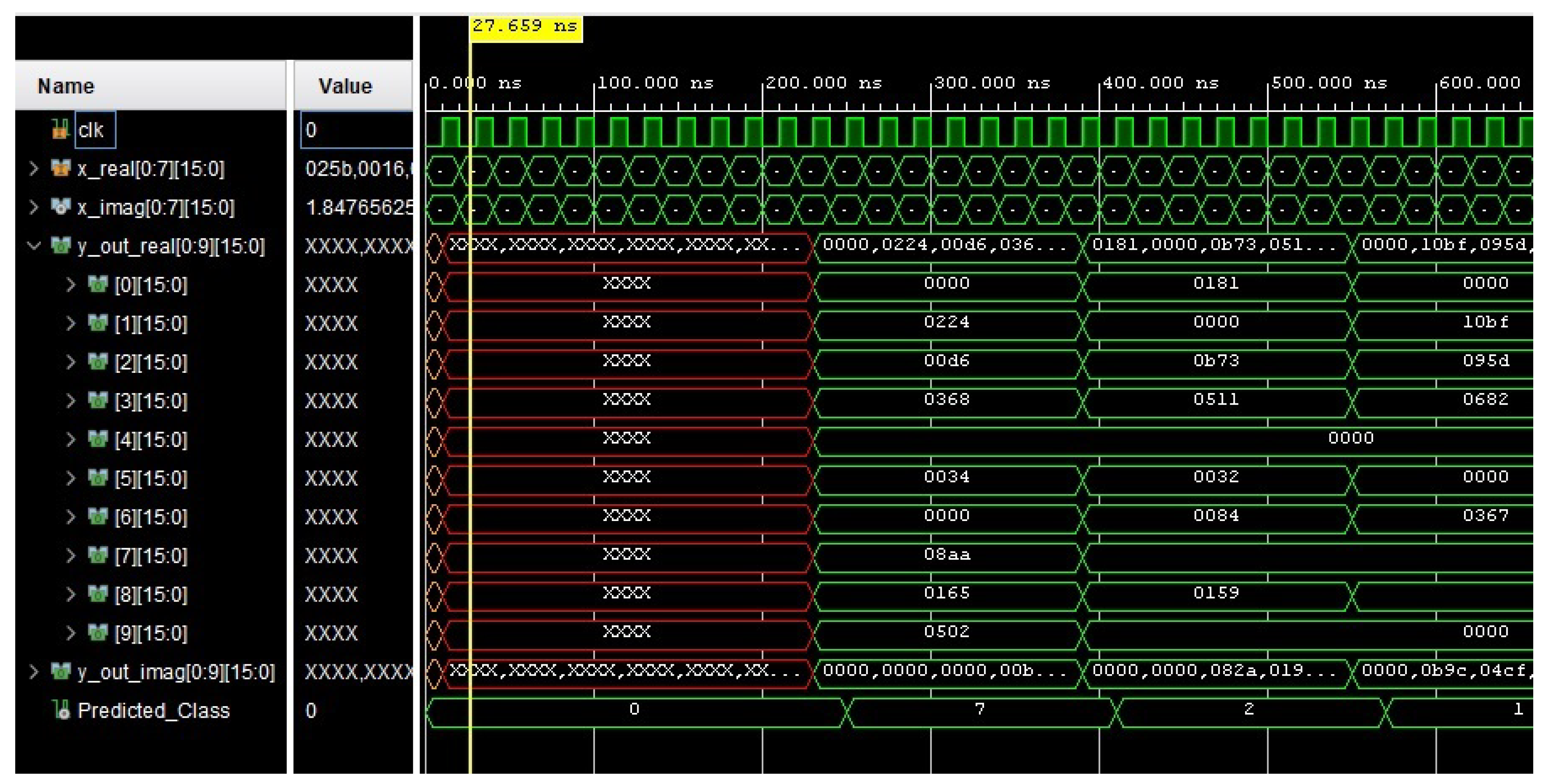
Figure 9 presents the behavioral simulation report for CVNN_64, which refers to the Complex-valued Neural Network model implemented on FPGA catering to 64 data points of the polar-transformed MNIST dataset. Within the simulation window, the object termed Predicted_class displays the classification outcome for the complex-valued neural network model tailored for the FPGA, targeting the polar-transformed MNIST dataset with 64 data points. Comparable classification outcomes emerged for the other model variations.

6.1. Maximum Operating Frequency ( $F_{\max}$ )

The maximum operating frequency, denoted as

F_{\max}

, is a crucial metric derived from the Worst Negative Slack (WNS) present in Vivado’s “Timing Summary Report” post-synthesis and implementation.

In digital design, slack quantifies the deviation between the expected and actual arrival times of signals, as defined by the design’s timing constraints. A negative slack is indicative of a timing violation, suggesting that signals are not reaching their intended destinations within the desired time frame.

Of all the timing violations, the WNS represents the most pronounced delay across the entire design. A positive WNS implies that the design adheres to all its timing constraints. Conversely, a negative WNS is indicative of a breach in timing specifications, necessitating design modifications.

The effective clock period, adjusted based on the WNS, is computed as:

Adjusted Clock Period = T - WNS

Where T is the intended clock period.

Consequently,

F_{\max}

is derived using:

F_{\max} = \frac{1}{Adjusted Clock Period} = \frac{1}{T - WNS}

For illustrative purposes, if the reported WNS is -0.5ns and the target clock period T is 5ns, the effective clock period adjusts to 5.5ns. This results in a

F_{\max}

of approximately 181.82MHz, computed as

\frac{1}{5.5 ns}

It’s worth noting that alternative approaches exist to attain the desired target frequency beyond simply recalculating

F_{\max}

based on WNS. However, in the scope of this research, our emphasis was on determining

F_{\max}

using the WNS. Exploring these alternative strategies might be a point of interest for future work to refine and optimize the design.

During the course of our research, while the above formula provided a theoretical maximum frequency, we opted for a slightly reduced frequency to instate a safety margin. This precaution ensures the design remains resilient against potential timing constraint violations.

Following the generation of the post-implementation Timing reports for all models in Vivado, we tabulated the results, as shown in Table 7. The table summarizes the maximum clock period, the derived maximum operating frequency, and the Worst Negative Slack (WNS) for each of the models.

Table 7. Post-implementation Timing results for different neural network models on Vivado

Model	Max. Clock Period (ns)	Max. Freq. (MHz)	WNS (ns)
RVNN_64	8	125	0.155
CVNN_64	10.5	95.238	0.096
RVNN_128	8	125	159
CVNN_128	10	100	0.182
RVNN_Raw_MNIST	8	125	0.166

6.2. Benchmarking FPGA Inference Models Against CPU and GPU Platforms

To gauge the performance of our FPGA-based inference models, we benchmarked them against CPU and GPU-based models. For this comparison, we utilized the Google Colab platform, executing inference models implemented in the Python programming language. Below are the specifications of the computational environment we used:

Table 8. Computational environment specifications on Google Colab

Attribute	Specification
Platform	Google Colab
Operating System	Ubuntu 22.04.2 LTS
CPU	Intel(R) Xeon(R) CPU @ 2.00GHz
GPU	NVIDIA® Tesla® P4
Python Version	3.10.12

The ensuing table, Table 9, delineates the inference times, in seconds, for various neural network models. Each model inferred a total of 10,000 MNIST test datasets on both CPU and GPU environments in Google Colab. Five trials were conducted for each model and hardware platform, and the average results are presented in the table. Further details are provided in the Appendix.

Table 9. Inference times for neural network models on Google Colab’s CPU and GPU environments

Model	Inference Time (CPU, s)	Inference Time (GPU, s)
RVNN_64	0.43	0.3
CVNN_64	0.28	0.23
RVNN_128	0.44	0.36
CVNN_128	0.31	0.26
RVNN_Raw_MNIST	0.53	0.35

6.2.1. Inference time comparison

Table 7 provides insights into the maximum operating frequency for each implementation. To comprehensively understand the performance of our FPGA-based models, we derive the total inference time required to classify the 10,000 MNIST test dataset. The formula to compute this is delineated below:

Inder_time = T \times N \times S

(21)

Where:

T: Duration of each clock cycle in nanosecond.
N: Number of clock cycles needed to classify each sample.
S: Total number of samples, which is 10,000 in this case.

For our dataset configurations:

CVNN_64 and RVNN_64 each require 8 clock cycles to classify a sample.
CVNN_128 and RVNN_128 each necessitate 16 clock cycles to complete the classification of a sample.
RVNN_Raw_MNIST requires 49 clock cycles to classify a sample

Following our analysis, the inferred times for each model are summarized in Table 10:

Table 10. Inference times for neural network models on FPGA

Model	T×N×S	Inference Time (ns)
RVNN_64	8×8×10,000	640,000
CVNN_64	10.5×8×10,000	840,000
RVNN_128	8×16×10,000	1,280,000
CVNN_128	10×16×10,000	1,600,000
RVNN_Raw_MNIST	8×49×10,000	3,920,000

6.2.2. Inference Time Comparison across CPU, GPU, and FPGA

Table 11 shows the comparison of inference times in milliseconds for different models on varisous hardware platforms. To convey the concept of “how fast” a model is, we use the reciprocal of the inference time. In other words, we computed the “speed” as:

Speed = \frac{1}{Inference Time}

(22)

Table 11. Inference Times in milliseconds for Different Models on Various Hardware Platforms

Models	Inference Time (CPU, ms)	Inference Time (GPU, ms)	Inference Time (FPGA, ms)	Inference Time (CPU_2, ms)
RVNN_64	430	300	0.64	180
CVNN_64	280	230	0.84	210
RVNN_128	440	360	1.28	210
CVNN_128	310	260	1.6	230
RVNN_Raw_MNIST	530	350	3.92	240

This gives us a measure where larger values indicate faster performance. Note that for this metric, a higher value is better, which is the opposite of the inference time where a lower value is better. As shown in Equation 22, the speed is the inverse of the inference time.

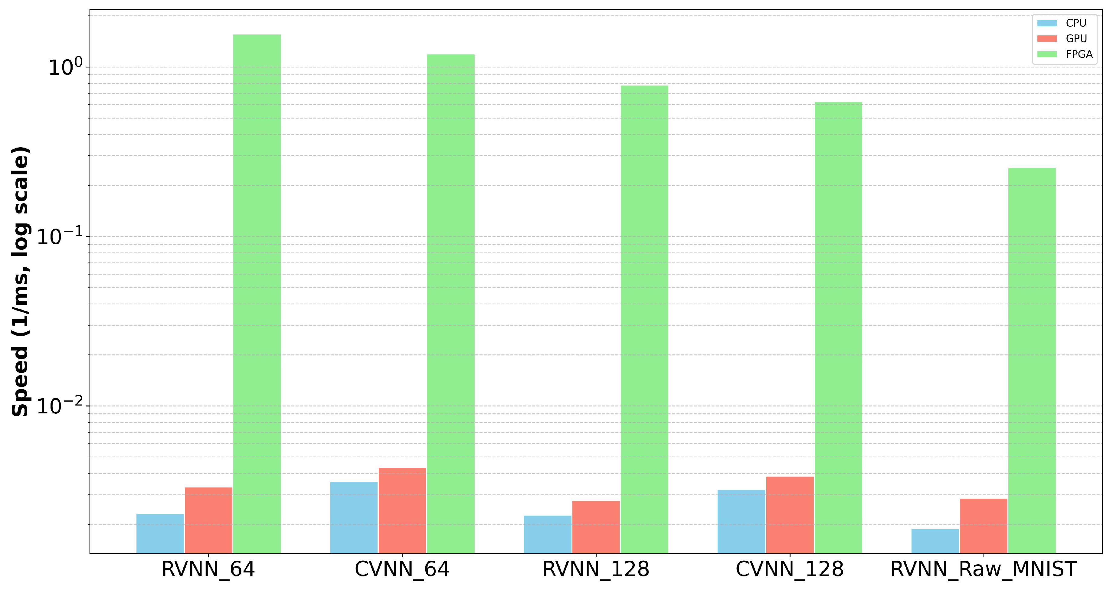
In our comparative analysis of neural network model speeds across CPU, GPU, and FPGA platforms, several distinct patterns emerged illustrated in the Figure 10. Most prominently, the FPGA demonstrated superior speeds when compared to both the CPU and GPU, underscoring its viability for tasks requiring swift computation. The GPU, with its parallel processing capabilities, showcased higher speeds relative to the CPU, signifying its prowess in neural network computations. However, it was the remarkable speed of the FPGA, especially for specific neural network architectures, that was most noticeable.

Diving deeper into the nuances of the model variants, the CVNN_64 and RVNN_64 models displayed considerably greater speeds compared to their CVNN_128 and RVNN_128 counterparts. This observation is intuitive: models with a reduced complexity and fewer parameters naturally lead to faster computation times. While we did not implement the RVNN_Raw_MNIST model on FPGA, when juxtaposed with the results from the FPGA models, it becomes evident that FPGAs substantially outperform the models using the original MNIST dataset.

This further suggests that the throughput for our CVNNs and RVNNs implemented on FPGA systems is superior to that of similar networks running on CPU or GPU-based systems.

In summation, our analysis emphasizes the critical role of hardware selection in maximizing neural network efficiency. Within this context, FPGAs emerge as an optimal choice, particularly when compared to models trained on traditional datasets.

6.2.3. Power Consumption Comparison

Understanding the power consumption of neural network models is crucial for their deployment in real-world scenarios, especially in power-sensitive applications. Our neural network designs, when implemented on FPGA, yielded power consumption results as detailed in Table 2.2.

Table 12. Power Consumption for Neural Network Models on FPGA

Model	Thermal Power	Static Power	Power Consumption
	(Watt per second)	(Watt per second)	(Watt per 10,000 frame)
RVNN_64	1.585	0.252	0.001014
CVNN_64	2.585	0.26	0.022167
RVNN_128	1.694	0.253	0.002168
CVNN_128	2.917	0.263	0.004656
RVNN_Raw_MNIST	2.53	0.274	0.009917

Interpretation of Power Metrics: Thermal power, often termed as the total on-chip power, is a summation of dynamic and static power. Dynamic power refers to the average power consumption during logic utilization and switching activities. Conversely, static power characterizes the scenario where the device remains active but abstains from any form of utilization or switching.

From Table 2.2, it is evident that RVNN models are more power-efficient compared to CVNN models. Moreover, models based on 64 input entries exhibit lower power consumption than their 128 input counterparts. However, FPGA implementation of Neural Network model (RVNN_Raw_MNIST) for unprocessed raw MNIST data consumed more than double power than most expensive neural network model (such as CVNN_128) for preprocessed data in classification of 10,000 frame of MNIST test dataset.

Comparison with CPU and GPU: Our attempt to directly compare FPGA-based power consumption with CPU and GPU systems encountered a challenge. Google Colab, which was employed for CPU and GPU-based designs, doesn’t furnish direct power consumption metrics. However, resorting to the respective processor datasheets, we discerned their TDP (Thermal Design Power) ratings. The Intel(R) Xeon(R) CPU @ 2.00GHz employed by Colab boasts a TDP of 270 watts [33], whereas its GPU, the NVIDIA® Tesla® P4, has a TDP of 75 watts [34].

Further exploration led us to test on a multi-core CPU-based laptop powered by the 11th Gen Intel(R) Core(TM) i5-1135G7 @ 2.40GHz processor. This processor’s datasheet indicates a power consumption of approximately 25 watts in its Low Power Mode [35].

Han J. et al. [21] developed a spiking neural network model for FPGA platforms, and similarly implemented it in Python for NVIDIA Tesla P100 GPU. In their experiments processing 10,000 frames from the MNIST test dataset, the GPU implementation required 7.96 seconds and averaged 29.6 watts of power consumption. Contrastingly, our CVNN_128 model showcases superior efficiency, consuming merely 2.917 watts per second and completing the same task in a swift 1.6 milliseconds. This performance not only makes our system almost 100 times faster than the GPU-based solution but also achieves around ten times greater power efficiency.

Literature provides further insights. Research shows that contemporary laptops generally consume power in the range of 8 to 30 watts [36]. Another study, utilizing a shunt resistor with a laptop’s power supply, revealed that the Intel i7-4820K processor expends between 10-80 watts, contingent on the task [37].

Comparative analyses between CPU, GPU, and FPGA platforms for identical tasks have been conducted. One such study suggests that the Intel Core2 QX9650 CPU, NVidia GTX 280 GPU, and Xilinx xc5vlx330 FPGA consume maximum power of 170 watts, 178 watts, and 30 watts respectively [38]. Another comparison focused on energy efficiency for various vision kernels. In this study, the utilized CPU and GPU came equipped with on-board power measuring ICs. The results unequivocally demonstrated that the FPGA accelerator outperforms both GPU and CPU systems across all test cases [39].

Conclusion: The evidence compiled, both from our own implementations and the existing literature, robustly underscores FPGA’s prowess in energy efficiency, solidifying its position as a more power-conscious choice than conventional CPU and GPU systems.

6.2.4. Resource Utilization among different neural network models implemented on FPGA

This section delves into the resource utilization of various neural network models when implemented on the Virtex-7 VC707 Evaluation Platform, which features the xc7vx485tffg1761-2 FPGA chip. The neural network models under consideration include RVNN_64, CVNN_64, RVNN_128, and CVNN_128. In the context of FPGA implementations, the resources can be described as follows:

LUT (Look-Up Table): Used for implementing combinational logic functions.
FF (Flip-Flop): Represents sequential logic, storing binary values.
DSP (Digital Signal Processor): Useful for performing arithmetic operations, especially multiplication.
IO (Input-Output Port): Interfaces for the FPGA to communicate with external components.
BUFG (Global Buffer): Provides clock and reset signal distribution across the FPGA.

In the analysis of the resource utilization, CVNN_128 consistently demands the most resources, particularly in LUTs and FFs, while RVNN_64 remains the least resource-intensive. DSP utilization is highest for CVNN_64 and CVNN_128, and IO consumption is fairly consistent across models, with a minor edge for CVNN_64. Notably, all models have minimal BUFG consumption, utilizing only a fraction of what’s available.

Table 13. Resource Utilization among different neural network models

Resource	RVNN_64	CVNN_64	RVNN_128	CVNN_128	RVNN_Raw_MNIST	Available
LUT	9,123	17,723	13,122	24,164	20,993	303,600
FF	3,110	5,936	5,703	11,520	16,066	607,200
BRAM	-	-	-	-	160	1,030
DSP	485	1,333	469	1,333	507	2,800
IO	417	577	417	577	417	700
BUFG	1	1	1	1	1	32

6.2.5. Evaluation with Existing Result

Until now, we have come across just one FPGA-based complex-valued neural network model, published in May 2023. However, it should be noted that this model was not applied to MNIST or image classification tasks, making it incomparable to our research.

To assess our findings in the context of existing work, we selected two distinct neural network models (SNN[18] and CNN[40]) implemented on FPGA for MNIST classification. In Table 14, we present a performance comparison among these three FPGA-based neural network models for MNIST digit classification.

Table 14. Comparative Analysis of Different Neural Network Models on FPGA

Models	Accuracy	Inference Time	Power (watt per second)	(watt per 10,000 frame)
SNN	90.39%	1s	1.131W	1.131W
CNN	94.43%	0.127s	4.5W	0.5715W
CVNN_128	88.3%	0.0016s	2.91W	0.004656W
CVNN_64	87.0%	0.00084s	2.58W	0.002167W

In recent publications, a spiking neural network (SNN) by Zhang J et el. [18] published in May 2023 and a convolutional neural network (CNN) by Parra D. et el. [40] published in October 2023 achieved accuracy rates of 90.39% and 94.43%, respectively, on the MNIST test dataset. Our model, CVNN_128, achieved an accuracy of 88.3% on the same dataset. Comparing power consumption, the SNN, CNN, and CVNN_128 models consumed 1.131W, 0.5715W, and 0.004656W, respectively, for the 10,000 frames of the MNIST test dataset. Despite its slightly lower accuracy, CVNN_128 stands out for its significantly lower power consumption (almost 122 times less than CNN and 240 times less than SNN) and exceptional speed (thousands of times faster than SNN and over hundred times faster than CNN).

Table 15. Resource Utilization for Different Neural Network Models on FPGA

Resource	SNN	CNN	CVNN_128
LUT	73,677	6,373	24,164
LUTRAM	3,669	71	0
FF	32,853	12,470	11,520
BRAM	0	0	0
DSP	10	93	1,333
IO	419	18	577
BUFG	1	0	1

Table 15 provides a comparison of resource utilization on FPGA for the SNN, CNN, and CVNN_128 models. It’s evident that the SNN consumes more resources than CNN and CVNN. CNN exhibits the most efficient resource utilization among them. It’s important to note that these are three distinct models, each optimized differently, making a direct comparison challenging. Nevertheless, the resource utilization table offers a general idea of the differences in their designs.

In summary, our CVNN_128 model showcases remarkable improvements in both energy efficiency and processing speed when compared to recently published models. We believe that the integration of polar representation for 2D images and complex-valued neural networks on FPGA holds great promise for energy-constrained environments, offering faster processing capabilities.

7. Discussion and Conclusion

This research set out to explore the implementation of CVNNs for polar-represention of 2D image classification on FPGA. The primary objectives were to assess the effectiveness of CVNNs in this context and to evaluate the performance benefits of FPGA-based implementations.

The results indicate a notable performance in the classification accuracy of the polar-represented MNIST dataset using CVNNs. In our comparative analysis against Real-valued Neural Networks (RVNNs), we observed that the CVNN model with 128 input datapoints (CVNN_128) achieved a classification accuracy 0.8 percent higher than its RVNN counterpart, RVNN_128. Furthermore, with a more reduced number of input datapoints (64 datapoints), CVNN_64 exhibited a 1.1 percent higher classification accuracy when compared to RVNN_64 in the context of processing polar-represented MNIST handwritten digit test dataset. These findings align with our initial hypothesis, demonstrating that complex-valued networks excel in handling polar-represented image data. This superiority arises from CVNN’s ability to learn correlations between magnitude and phase information in complex data, resulting in improved performance compared to RVNNs. The use of FPGAs for implementation further enhanced the computational efficiency, showcasing the potential of hardware acceleration in neural network processing.

Comparatively, the FPGA implementation demonstrated improvements in processing speed and power efficiency. Our research reveals that our robust design, CVNN_128, is approximately 200 times faster than a CPU-based computer running CVNN and 150 times faster than a GPU-based computer for MNIST digit classification. Additionally, it demonstrates lower power consumption when compared to CPU and GPU-based systems, as well as other neural network models implemented on FPGA for MNIST digit classification.This supports the hypothesis that FPGA-based systems can provide significant advantages in specific neural network applications, particularly in scenarios where low power consumption and high-speed computation are crucial.

7.1. Limitations of the Study

The study was limited to the MNIST handwritten digits dataset, which may constrain the generalizability of the findings to other types of datasets.

7.2. Recommendations for Future Research

Further research should extend the validation of polar-represented image classification using Complex-Valued Neural Networks (CVNNs) beyond the MNIST dataset to include a wider array of 2D images. This expansion would test the model’s generalizability and effectiveness across diverse image sets.

Exploring the use of Spiking Neural Networks (SNNs) for polar-represented image data also presents a valuable opportunity. A comparative analysis between SNN and CVNN performance could offer deeper insights into the potential benefits of each neural network type for specific image classification tasks. Since the reprocessing technique was primarily thought for SNNs.

Finally, the optimization of CVNN implementation on FPGAs warrants continued effort, particularly through enhanced pipelining techniques, which could significantly improve computational throughput and energy efficiency. Such advancements could bring FPGA-based CVNNs to the forefront of practical applications, where resource optimization is paramount.

7.3. Conclusion

This research highlights the possibilities of using polar representation of 2D images and complex-valued neural networks through FPGA-based implementations for image classification tasks. The results provide valuable insights into the realm of neural network acceleration and pave the way for further exploration into hardware-accelerated machine learning.

Author Contributions

“Conceptualization, M.A. and L.Z.; methodology, M.A. and L.Z.; software, M.A.; validation, M.A. and M.E.H.C.; formal analysis, M.A.; investigation, M.A. and M.E.H.C.; resources, L.Z.; data curation, M.A.; writing—original draft preparation, M.A.; writing—review and editing, L.Z. and M.E.H.C.; visualization, M.A.; supervision, L.Z.; project administration, L.Z.; All authors have read and agreed to the published version of the manuscript.

Funding

This research received no external funding.

Institutional Review Board Statement

N/A

Informed Consent Statement

N/A

Data Availability Statement

Data sharing not applicable

Acknowledgments

N/A

Conflicts of Interest

The authors declare no conflict of interest.

Abbreviations

The following abbreviations are used in this manuscript:

FPGA	Field-Programmable Gate Array
MNIST	Modified National Institute of Standards and Technology
ASIC	Application-Specific Integrated Circuit
DFT	Discrete Fourier Transform
CVNNs	Complex-Valued Neural Networks
RVNNs	Real-Valued Neural Networks
SNN	Spiking Neural Network
VHDL	VHSIC Hardware Description Language
VHSIC	Very High Speed Integrated Circuit
DFT	Discrete Fourier Transform
GPU	Graphics Processing Unit
CPU	Central Processing Unit
MLPs	Multi-Layer Perceptrons
RNNs	Recurrent Neural Networks
CNNs	Convolutional Neural Networks

Appendix A. Polar-coordinate representation details

Appendix A.1. Logarithmic Transform

Pixel intensity perception in the human visual system is non-linear. Contrary to a straightforward linear response, the human eye exhibits a logarithmic sensitivity to brightness variations. This implies that the perceptual distinction between two pixel intensities doesn’t align directly with their numerical disparity. In essence, the human eye is more adept at discerning variations in low-intensity regions compared to those in brighter or high-intensity areas. 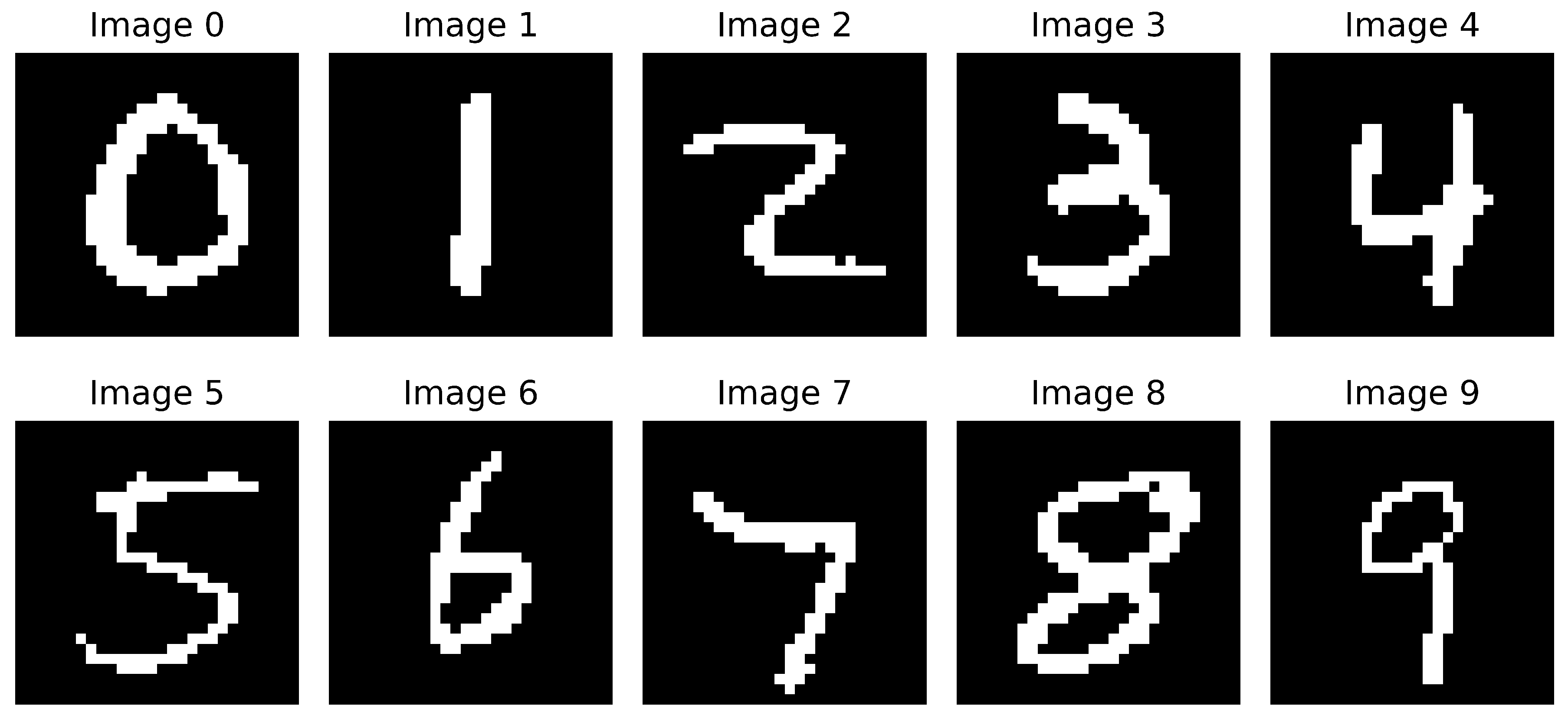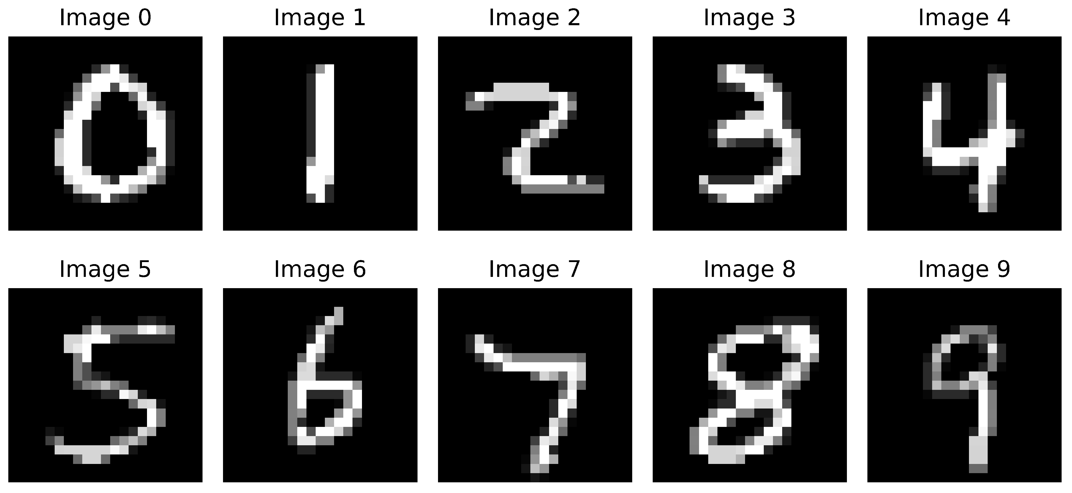Such an observation is supported by the Weber-Fechner law[41]. With this understanding, numerous technologies tailored for image processing are designed to optimize visuals for human perception. To achieve this, we transitioned the image encoding from a 0-256 scale to a 0-8 level priority encoding. The calculation of

{log}_{2} (P) = 8

is employed to identify pixels with the highest intensity level, as depicted in Figure A1. The priority encoding technique notably amplifies the contrast of the source images.

Figure A1. 0-9 MNIST handwritten digits with level-8 intensity

Figure A2. 0-9 MNIST handwritten digits with level-8 intensity and highlighted contour

Appendix A.2. Highlighted Contour

Following the logarithmic transformation to an eight-level intensity, all intensity levels, with the exception of the 8th level, are reduced to zero, resulting in a prominently highlighted contour. This contour effectively captures and depicts the most crucial details and shapes[42], as illustrated in Figure A2. By nullifying other intensity levels, there is a significant reduction in data volume, thereby enhancing the efficiency and speed of subsequent algorithms.

Appendix A.3. Downsampling

Downsampling in two-dimensional imagery can be conceptualized as a spatial reduction, where the resolution is systematically decreased across both dimensions[43].

In 2D image downsampling, an image matrix

I (x, y)

is reduced to

I_{d} (x^{'}, y^{'})

using:

I_{d} (x^{'}, y^{'}) = I (D_{x} \times x^{'}, D_{y} \times y^{'})

(A1)

Where

D_{x}

and

D_{y}

are the down-sampling factors for width and height, respectively.

In the current work, given that the MNIST images possess a resolution of

28 \times 28

, we adopted two specific down-sampling approaches. For a dataset encompassing 64 data points, the down-sampling coefficients were designated as

D_{x} = D_{y} = 2

. For a dataset of 128 data points, the coefficients were adjusted to

D_{x} = D_{y} = \frac{4}{3}

. The rationale and intricacies behind these choices are pivotal to our research objectives and will be elaborated upon in the following sections. Figure A3 depicts the 0-9 MNIST numbers after down-sampling with a factor of 4/3.

Figure A3. 10 MNIST level-8 intensity images after down-sampled

Appendix A.4. Polar Coordinate Representation

The polar transform of a 2D image shifts the image’s representation from the Cartesian coordinate system to the polar coordinate system. In the Cartesian system, each pixel’s position is denoted by x and y coordinates. In contrast, in the polar system, pixel locations are characterized by magnitude

ρ

and phase

θ

. Here, the magnitude signifies the radial distance of a pixel from the center of the polar plane, while the phase indicates the pixel’s angle or orientation.

The polar representation offers several advantages in image processing and analysis. For instance, the polar transform is instrumental in frequency analysis and pattern recognition within images. In this context, the radial distance in the polar plane can be interpreted as a frequency magnitude, and the pixel’s orientation as its phase. These attributes are beneficial for tasks such as noise reduction, feature segmentation, and image compression [44]. Moreover, the polar format accentuates radial lines and concentric circles, enhancing the visualization of textures, facilitating fingerprint analysis, and aiding in object detection within an image [45].

In the process of converting image coordinates from Cartesian to polar representation, given an image’s Cartesian coordinates

(x, y)

with the origin centered in the image, the corresponding polar coordinates

(ρ, θ)

are determined using the equations

ρ = \sqrt{x^{2} + y^{2}}

and

θ = arctan 2 (y, x) .

Initially, the image’s dimensions are ascertained, and its center is computed. A meshgrid, representing the x and y coordinates of each pixel, is then generated and adjusted to have the origin at the image’s center. Subsequently, for each pixel, the polar coordinates are calculated. Only pixels with intensity values greater than 0 are considered, and their corresponding polar coordinates are stored in the theta_rho_pairs list. This transformation, implemented in Python with the NumPy library, efficiently captures the polar coordinates of all non-black pixels in the image.

Algorithm 1:Cartesian to Polar Conversion Algorithm

1:: procedureCartesianToPolar(img)
2:: $rows \leftarrow img . height$
3:: $cols \leftarrow img . width$
4:: $centerX \leftarrow cols / 2$
5:: $centerY \leftarrow rows / 2$
6:: $X, Y \leftarrow CreateMeshgrid (1 to cols, 1 to rows)$
7:: $X \leftarrow X - centerX$
8:: $Y \leftarrow centerY - Y$
9:: $θ \leftarrow CalculateAngle (Y, X)$
10:: $ρ \leftarrow CalculateDistance (X, Y)$
11:: $theta_rho_pairs \leftarrow EmptyList ()$
12:: for $i from 0 to rows - 1$ do
13:: for $j from 0 to cols - 1$ do
14:: if $img [i, j] > 0$ then
15:: $theta_rho_pairs . append ([θ [i, j], ρ [i, j]])$
16:: end if
17:: end for
18:: end for
19:: return $theta_rho_pairs$
20:: end procedure

Following the polar transformation, we subjected the magnitude values of the image data to normalization. This step ensures that the magnitude values reside within a designated range, establishing uniformity in the radial distances. This uniformity is crucial for subsequent computational processes and offers enhanced visualization clarity.

Figure A4. Illustration of Polar transformed MNIST 0-9 images

In the polar representation of an image, it is depicted as a sequence of complex exponential values, denoted as

P (ρ, θ) = ρ e^{i θ}

. In this context,

θ

stands for the angle or phase, spanning from

- π

π

, and

ρ

indicates the magnitude or radial distance.

Histogram Analysis: To select the optimal number of data points for the serialization and Fourier Transform of polar-transformed images, we performed a histogram distribution analysis. This analysis utilized 10,000 test images and 60,000 training images to assess the number of data points present in each image.

Figure A5. Distribution of data points for all train and test images

The histograms presented in Figure A5 elucidate the distribution of data points for both training and testing images. Upon close inspection of these figures, it becomes evident that the predominant number of data points for both sets of images hovers around 150. In light of this observation, an optimal data point threshold,

N = 128

, was established for subsequent analyses, a decision informed by the histogram assessments.

Appendix A.5. Zero-Padding and Decimation

To standardize the data point counts across images:

Images with fewer than 128 data points were subjected to zero-padding to achieve a consistent count of 128.
On the other hand, images with data points surpassing 128 underwent decimation to bring their count down to the stipulated 128.

The rationale behind setting

N = 128

was multifaceted. Opting for a threshold of 150 would have necessitated extensive zero-padding for a vast number of images, potentially introducing extraneous noise. Conversely, a threshold considerably below 128 risked omitting vital image information. The selected threshold of 128 adeptly balances these considerations, ensuring data uniformity across images while retaining their inherent distinctiveness. The combined approach of zero-padding and decimation guarantees that all images, irrespective of their original dimensions or data point counts, adhere to this standardized threshold.

It is important to highlight that following the extraction of the highlighted contour from the 2D MNIST image, and before proceeding with the polar transformation, an intermediate decimation step was introduced. At this juncture, a decimation factor of

\frac{4}{3}

was applied, facilitating the selection of 128 data points for our subsequent analysis. This choice was informed by our earlier observations and the need for a balanced representation of the image data. In a similar vein, a decimation factor of 2 was employed to refine our selection further to 64 data points. This additional selection was made to provide a more compact representation, while still capturing essential image features. Consequently, both 128 and 64 data points were chosen for in-depth analysis. These two distinct data point sets, 128 and 64, were uniformly adopted throughout our research, ensuring a consistent methodology and laying the groundwork for comparative evaluations.

Figure A6. Polar transformed 0-9 MNIST image where N=128,

ρ

=[0,1]

Figure A6. Polar transformed 0-9 MNIST image where N=128,

ρ

=[0,1]

Figure A7. Polar transformed 0-9 MNIST image where N=64,

ρ

=[0,1]

Figure A7. Polar transformed 0-9 MNIST image where N=64,

ρ

=[0,1]

Figure A6 illustrates the polar-transformed MNIST images, ranging from 0 to 9, after selecting 128 data points. Furthermore, as observed in Figure A7, even with a reduced set of 64 data points, the visualization still conveys discernible information.

Appendix A.6. Serialization

The primary motivation behind the polar transformation of 2D MNIST images was to devise a phase encoding technique tailored for the spiking neural network (SNN). In this approach, individual spiking neurons symbolize unique frequency components of the image. Notably, phase encoding has demonstrated a significant speed advantage over rate encoding [46].

While our study does not delve into the implementation of SNNs, our aim is to harness this encoded data within a complex-valued neural network. This will allow us to gauge both the efficacy of the encoded data and the performance of our model. The serialization of the polar-represented image is a two-fold process. Initially, the polar data is translated to its complex representation using the Euler’s formula:

z = ρ \times e^{i θ}

Here, z stands for the complex number,

ρ

represents the magnitude, and

θ

is the angle in polar coordinates [47].

Subsequently, the Discrete Fourier Transform (DFT) is applied. DFT serves as a mathematical tool that transforms a sequence (typically time-domain signals) into its constituent frequency components. The outcome is a series of complex numbers, each signifying the amplitude and phase of a specific frequency component in the original sequence. In our methodology, this transformation yields N complex coefficients using the formula:

X [k] = \sum_{n = 0}^{N - 1} x [n] \cdot e^{- i \frac{2 π k n}{N}}

(A2)

Where:

$X [k]$ denotes the output in the frequency domain corresponding to the frequency index k.
$x [n]$ represents the time domain samples.
N is the total number of these samples.
n is an index running through the time samples, ranging from 0 to $N - 1$ .
k is an index for the frequency components, also ranging from 0 to $N - 1$ .

Figure A8. DFT coefficient (magnitude) - N=128

Figure A9. DFT coefficient (Phase) - N=128

Appendix A.7. Complex-valued Neural Network (CVNN) implementation

CVNNs! (CVNNs!) represent a specialized class of neural networks that operate on complex numbers, encompassing both real and imaginary components [23]. While conventional neural networks primarily deal with real-valued data, CVNNs have gained prominence in applications where data inherently exhibits both magnitude and phase information, especially those involving signals, waves, or data with phase information. The deployment of complex numbers within neural networks is of particular relevance to this research, as it addresses the unique challenges posed by the preprocessed MNIST handwritten digits dataset. In the context of this study, the relevance of CVNNs stems from their intrinsic capability to effectively process complex-valued data. The research is focused on the preprocessed MNIST dataset, which undergoes a transformation from Cartesian to polar coordinates, followed by serialization using the discrete Fourier transform (DFT). This transformation equips the dataset with complex numbers, enabling a more compact representation while retaining critical phase information, which is essential for character recognition tasks [24].

References

Haase, J.; Hanel, P.H. Artificial muses: Generative artificial intelligence chatbots have risen to human-level creativity. arXiv preprint arXiv:2303.12003 2023. [CrossRef]
OpenAI. ChatGPT. https://chat.openai.com/ Accessed: 07 November 2023.
Miller, A.I. The artist in the machine: The world of AI-powered creativity; Mit Press, 2019.
Midjourney, Inc. Midjourney. https://www.midjourney.com/ Accessed on 07 November 2023.
Egmont-Petersen, M.; de Ridder, D.; Handels, H. Image processing with neural networks—a review. Pattern recognition 2002, 35, 2279–2301. [CrossRef]
Chen, Y.H.; Krishna, T.; Emer, J.S.; Sze, V. Eyeriss: An Energy-Efficient Reconfigurable Accelerator for Deep Convolutional Neural Networks. IEEE Journal of Solid-State Circuits 2017, 52, 127–138. [CrossRef]
Wang, C.; Luo, Z. A Review of the Optimal Design of Neural Networks Based on FPGA. Applied Sciences 2022, 12. [CrossRef]
Zhang, L. Polar Representation of 2D Image Using Complex Exponential Spiking Neuron Network. Proceedings of the 52nd International Conference on Parallel Processing Workshops, 2023, pp. 180–186. [CrossRef]
LeCun, Y.; Cortes, C.; Burges, C.; others. MNIST handwritten digit database, 2010.
Touvron, H.; Bojanowski, P.; Caron, M.; Cord, M.; El-Nouby, A.; Grave, E.; Izacard, G.; Joulin, A.; Synnaeve, G.; Verbeek, J.; others. Resmlp: Feedforward networks for image classification with data-efficient training. IEEE Transactions on Pattern Analysis and Machine Intelligence 2022, 45, 5314–5321. [CrossRef]
Dhruv, P.; Naskar, S. Image classification using convolutional neural network (CNN) and recurrent neural network (RNN): A review. Machine Learning and Information Processing: Proceedings of ICMLIP 2019 2020, pp. 367–381. [CrossRef]
Pak, M.; Kim, S. A review of deep learning in image recognition. 2017 4th international conference on computer applications and information processing technology (CAIPT). IEEE, 2017, pp. 1–3. [CrossRef]
Rawat, S.; Rana, K.; Kumar, V. A novel complex-valued convolutional neural network for medical image denoising. Biomedical Signal Processing and Control 2021, 69, 102859. [CrossRef]
Scarnati, T.; Lewis, B. Complex-valued neural networks for synthetic aperture radar image classification. 2021 IEEE Radar Conference (RadarConf21). IEEE, 2021, pp. 1–6. [CrossRef]
Özkan Bakbak, P.; Peker, M. Classification of sonar echo signals in their reduced sparse forms using complex-valued wavelet neural network. Neural Computing and Applications 2020, 32, 2231–2241. [CrossRef]
Nurvitadhi, E.; Venkatesh, G.; Sim, J.; Marr, D.; Huang, R.; Ong Gee Hock, J.; Liew, Y.T.; Srivatsan, K.; Moss, D.; Subhaschandra, S.; Boudoukh, G. Can FPGAs Beat GPUs in Accelerating Next-Generation Deep Neural Networks? Proceedings of the 2017 ACM/SIGDA International Symposium on Field-Programmable Gate Arrays; Association for Computing Machinery: New York, NY, USA, 2017; FPGA ’17, p. 5–14. [CrossRef]
Wu, Y. Review on FPGA-Based Accelerators in Deep learning. 2023 IEEE 6th Information Technology,Networking,Electronic and Automation Control Conference (ITNEC), 2023, Vol. 6, pp. 452–456. [CrossRef]
Zhang, J.; Zhang, L. Spiking Neural Network Implementation on FPGA for Multiclass Classification. 2023 IEEE International Systems Conference (SysCon), 2023, pp. 1–8. [CrossRef]
Cho, M.; Kim, Y. Implementation of Data-optimized FPGA-based Accelerator for Convolutional Neural Network. 2020 International Conference on Electronics, Information, and Communication (ICEIC), 2020, pp. 1–2. [CrossRef]
Zhou, Y.; Jiang, J. An FPGA-based accelerator implementation for deep convolutional neural networks. 2015 4th International Conference on Computer Science and Network Technology (ICCSNT), 2015, Vol. 01, pp. 829–832. [CrossRef]
Han, J.; Li, Z.; Zheng, W.; Zhang, Y. Hardware implementation of spiking neural networks on FPGA. Tsinghua Science and Technology 2020, 25, 479–486. [CrossRef]
Lu, Y.; Yu, L.; Wei, X.; Hu, Y.; Yao, C. Lightweight 5G OFDM Channel Estimation Method Based on Deep Complex-Valued Neural Network, 2023. Available at SSRN 4436254.
Trabelsi, C.; Bilaniuk, O.; Zhang, Y.; Serdyuk, D.; Subramanian, S.; Santos, J.F.; Mehri, S.; Rostamzadeh, N.; Bengio, Y.; Pal, C.J. Deep Complex Networks, 2018, [arXiv:cs.NE/1705.09792]. [CrossRef]
Zhou, Y.; Wang, H.; Xu, F.; Jin, Y.Q. Polarimetric SAR Image Classification Using Deep Convolutional Neural Networks. IEEE Geoscience and Remote Sensing Letters 2016, 13, 1935–1939. [CrossRef]
Barrachina, J.A.; Ren, C.; Vieillard, G.; Morisseau, C.; Ovarlez, J.P. Theory and Implementation of Complex-Valued Neural Networks, 2023, [arXiv:stat.ML/2302.08286]. [CrossRef]
Amin, M.F.; Amin, M.I.; Al-Nuaimi, A.Y.H.; Murase, K. Wirtinger Calculus Based Gradient Descent and Levenberg-Marquardt Learning Algorithms in Complex-Valued Neural Networks. International Conference on Neural Information Processing. Springer Berlin Heidelberg, 2011, pp. 550–559. [CrossRef]
Nitta, T. An Extension of the Back-propagation Algorithm to Complex Numbers. Neural Networks 1997, 10, 1391–1415. [CrossRef]
Benvenuto, N.; Piazza, F. On the Complex Backpropagation Algorithm. IEEE Transactions on Signal Processing 1992, 40, 967–969. [CrossRef]
Barrachina, J.A. Complex-Valued Neural Networks (CVNN), 2019. Accessed: year-month-day. https://github.com/NEGU93/cvnn.
Byerly, A.; Kalganova, T.; Dear, I. No routing needed between capsules. Neurocomputing 2021, 463, 545–553. [CrossRef]
Brown, S.; Rose, J. FPGA and CPLD architectures: a tutorial. IEEE Design & Test of Computers 1996, 13, 42–57. [CrossRef]
Lacey, G.; Taylor, G.W.; Areibi, S. Deep Learning on FPGAs: Past, Present, and Future, 2016, [arXiv:cs.DC/1602.04283]. [CrossRef]
Intel. Product Brief, 3rd Gen Intel® Xeon® Scalable processors, 2023.
NVIDIA. Product Brief, TESLA P4 GPU ACCELERATOR, 2023.
Intel. 11th Generation Intel® Core™ Processor Family, Technical Resources: Intel® Core™ Processors.
Mahesri, A.; Vardhan, V. Power Consumption Breakdown on a Modern Laptop. Power-Aware Computer Systems; Falsafi, B.; VijayKumar, T.N., Eds.; Springer Berlin Heidelberg: Berlin, Heidelberg, 2005; pp. 165–180. [CrossRef]
Travers, M. CPU power consumption experiments and results analysis of Intel i7-4820K. Master’s thesis, Newcastle University, 2015.
Thomas, D.B.; Howes, L.; Luk, W. A Comparison of CPUs, GPUs, FPGAs, and Massively Parallel Processor Arrays for Random Number Generation; Association for Computing Machinery: New York, NY, USA, 2009; FPGA ’09, p. 63–72. [CrossRef]
Qasaimeh, M.; Denolf, K.; Lo, J.; Vissers, K.; Zambreno, J.; Jones, P.H. Comparing Energy Efficiency of CPU, GPU and FPGA Implementations for Vision Kernels. 2019 IEEE International Conference on Embedded Software and Systems (ICESS), 2019, pp. 1–8. [CrossRef]
Parra, D.; Escobar Sanabria, D.; Camargo, C. A Methodology and Open-Source Tools to Implement Convolutional Neural Networks Quantized with TensorFlow Lite on FPGAs. Electronics 2023, 12. [CrossRef]
Hecht, S. The Visual Discrimination of Intensity and the Weber-Fechner Law. The Journal of General Physiology 1924, 7, 235. [CrossRef]
Arbeláez, P.; Maire, M.; Fowlkes, C.; Malik, J. Contour Detection and Hierarchical Image Segmentation. IEEE Transactions on Pattern Analysis and Machine Intelligence 2011, 33, 898–916. [CrossRef]
Woods, R.E.; Gonzalez, R.C. Digital Image Processing; Pearson Education Ltd, 2008.
Gonzalez, R.C.; Woods, R.E. Digital Image Processing (3rd ed.); Prentice Hall, 2008.
Sonka, M.; Hlavac, V.; Boyle, R. Image Processing, Analysis and Machine Vision; Springer, 2013.
Kim, J.; Kim, H.; Huh, S.; Lee, J.; Choi, K. Deep neural networks with weighted spikes. Neurocomputing 2018, 311, 373–386. [CrossRef]
Oppenheim, A.V. Discrete-time Signal Processing; Pearson Education India, 1999.

Figure 1. Graphical Abstract of this research

Figure 2. MNIST digits and its polar transformed and serialized view (A) 0-9 original MNIST handwritten digits images, (B) Illustration of Polar transformed MNIST 0-9 images, (C) Polar transformed 0-9 MNIST image where N=128,

ρ

=[0,1], (D) Polar transformed 0-9 MNIST image where N=64,

ρ

=[0,1], (E) DFT coefficient (magnitude) - N=128, and (F) DFT coefficient (Phase) - N=128

ρ

=[0,1], (D) Polar transformed 0-9 MNIST image where N=64,

ρ

=[0,1], (E) DFT coefficient (magnitude) - N=128, and (F) DFT coefficient (Phase) - N=128

Figure 3. Testing Accuracy vs. Number of Hidden Layer Neurons

Figure 4. Testing accuracy of various neural network models on the MNIST dataset

Figure 5. Testing accuracy of different neural network models across various neuron counts in the hidden layer.

Figure 6. Typical Inference Structure of the CVNNs.

Figure 7. (A) Data flow diagram of the proposed Neural Network models on FPGA and (B) Primary schematic diagram of a single neuron implemented on FPGA

Figure 8. Schematic diagram of (A) complex-valued multiplier and (B) CReLU Activation in FPGA

Figure 9. Behavioural Simulation result of CVNN_64

Figure 10. Speed Across Different Hardware Platforms (Log Scale)

Disclaimer/Publisher’s Note: The statements, opinions and data contained in all publications are solely those of the individual author(s) and contributor(s) and not of MDPI and/or the editor(s). MDPI and/or the editor(s) disclaim responsibility for any injury to people or property resulting from any ideas, methods, instructions or products referred to in the content.

© 2023 by the authors. Licensee MDPI, Basel, Switzerland. This article is an open access article distributed under the terms and conditions of the Creative Commons Attribution (CC BY) license (http://creativecommons.org/licenses/by/4.0/).

Copyright: This open access article is published under a Creative Commons CC BY 4.0 license, which permit the free download, distribution, and reuse, provided that the author and preprint are cited in any reuse.

MDPI Initiatives

Important Links

Choose an area of interest and we will send you notifications of new preprints at your preferred frequency.

Disclaimer

FPGA Implementation of Complex-Valued Neural Network for Polar-Represented Image Classification

Abstract

1. Introduction

1.1. Related Workd

1.2. Research Objectives

1.3. Outline

2. Cartesian to Polar coordinate representation

3. Complex-valued Neural Network (CVNN) implementation

3.1. Complex Numbers in Neural Networks

3.2. Architectural Choices for CVNN:

3.3. CVNN Model

3.4. Training Procedure and Hyperparameters

3.4.1. The parameters for the feedforward model are configured as follows:

3.4.2. The training parameters for the CVNN are configured as follows:

3.5. Experimental Setup

3.5.1. Hardware and Software Environment

3.5.2. Dataset and Model Variations

3.5.3. Dataset Details

4. Results and Performance Evaluation

4.1. Accuracy Metrics

4.1.1. Graph Interpretation

4.1.2. Performance Insights

4.1.3. Justification for Selection of 20 Neurons

4.2. Comparison with Real-Valued Neural Networks

4.2.1. Objective & Hypothesis

4.2.2. Models Overview:

4.2.3. Processing Complex Data in Real-Valued Networks

4.2.4. Performance Insights

4.2.5. Testing accuracy cross various neuron counts

4.2.6. Comparison with Contemporary Research

4.3. Conclusion

5. FPGA Implementation of CVNNs

5.1. FPGA’s Role in Neural Network Acceleration

5.2. Complex-Valued Neural Network Inference Model

5.3. FPGA Implementation of Inference Model

5.3.1. Adder

5.3.2. Multiplier

5.3.3. Activation Functions

5.4. Fixed-Point Quantization for Neural Network Inference on FPGA

5.5. FPGA Structure for Our Neural Network Systems

6. Result and Evaluation of FPGA Implementation

6.1. Maximum Operating Frequency ( F max )

6.2. Benchmarking FPGA Inference Models Against CPU and GPU Platforms

6.2.1. Inference time comparison

6.2.2. Inference Time Comparison across CPU, GPU, and FPGA

6.2.3. Power Consumption Comparison

6.2.4. Resource Utilization among different neural network models implemented on FPGA

6.2.5. Evaluation with Existing Result

7. Discussion and Conclusion

7.1. Limitations of the Study

7.2. Recommendations for Future Research

7.3. Conclusion

Author Contributions

Funding

Institutional Review Board Statement

Informed Consent Statement

Data Availability Statement

Acknowledgments

Conflicts of Interest

Abbreviations

Appendix A. Polar-coordinate representation details

Appendix A.1. Logarithmic Transform

Appendix A.2. Highlighted Contour

Appendix A.3. Downsampling

Appendix A.4. Polar Coordinate Representation

Appendix A.5. Zero-Padding and Decimation

Appendix A.6. Serialization

Appendix A.7. Complex-valued Neural Network (CVNN) implementation

References

MDPI Initiatives

Important Links

Subscribe

6.1. Maximum Operating Frequency ( $F_{\max}$ )