Physics-Informed Neural Networks for the Condition Monitoring of Rotating Shafts

Preprint

Article

Physics-Informed Neural Networks for the Condition Monitoring of Rotating Shafts

Altmetrics

Downloads

151

Views

Comments

A peer-reviewed article of this preprint also exists.

This version is not peer-reviewed

Submitted:

22 November 2023

Posted:

23 November 2023

You are already at the latest version

Alerts

Abstract

Condition monitoring of rotating shafts is essential for ensuring the reliability and optimal performance of machinery in diverse industries. In this context, as industrial systems become increasingly complex, the need for efficient data processing techniques is paramount. Deep learning has emerged as a dominant approach due to its capacity to capture intricate data patterns and relationships. However, a prevalent challenge lies in the black-box nature of many deep learning algorithms, which often operate without adhering to the underlying physical characteristics intrinsic to the studied phenomena. To address this limitation and enhance the fusion of data-driven methodologies with the fundamental physics of the system under study, this paper leverages physics-informed neural networks (PINNs). Specifically, a simple but realistic numerical case study of an extended Jeffcott rotor model, encompassing damping effects and anisotropic supports for a more comprehensive modelling, is considered. PINNs are used for the estimation of five parameters that characterize the health state of the system. These parameters encompass the radial and angular position of the static unbalance due to the disk installed on the shaft, the stiffness along the principal axes of elasticity, and the non-rotating damping coefficient. The estimation is conducted solely by exploiting the displacement signals from the centre of the disk and, to showcase the efficacy and precision provided by this novel methodology, various scenarios involving different constant rotational speeds are examined. Additionally, the impact of noisy input data is also taken into account within the analysis.

Keywords:

Subject: Engineering - Mechanical Engineering

1. Introduction

Rotating shafts are elements of engineering systems that play a paramount role in the transmission of power, encompassing speed and torque, from one point to another [1], [2]. They are typically designed to endure substantial loads and to operate at high velocities, underscoring the need for precise alignment, equilibrium, and freedom from imperfections. These considerations are significant not only for enhancing the overall system performance, but also for improving its safety and reliability [3], [4]. To attain this objective, the practice of condition monitoring (CM) for rotating shafts allows continuously evaluating the shaft condition and performance and detecting any indications of malfunction or deterioration [5], [6]. Through the application of CM methodologies, potential issues can be promptly identified, and maintenance or repair actions can be driven to prevent accidents. This approach has shown to effectively mitigate the risk of unexpected downtime, reinforcing the overall system reliability [7], [8]. Furthermore, the widespread and cost-effective availability of sensors has revolutionized the acquisition of diagnostic signals, such as accelerations, strains, and elastic waves [9]. However, the availability of big data is itself a new layer of complexity, especially in the realm of signal processing. That is, the rapid expansion of the amount of acquired data has introduced the need for (i) improved hardware and software performance, and (ii) developing tools to deal with confounding factors, including those unrelated to the system health state, such as environmental and operational conditions [10], [11].

To tackle these challenges, deep learning has stood as a pivotal technological advancement in the CM of rotating machines, offering multifaced contributions of significant importance [12]. This approach has excelled in automatically extracting intricate patterns and features from raw sensor data, enhancing the precision and reliability of fault detection and anomaly characterization. As an example, the work in [13] applied deep learning to enhance wind turbine CM, addressing the data surge from increased wind farm units. By combining convolutional neural networks (CNNs) [14] and recurrent neural networks (RNNs) [15], it efficiently extracted features, reduced dimensionality, and provided effective CM, offering both real-time unit state checks and early warning capability, even amidst accidental parameter changes. In [16], a CM model based on CNNs for automatic fault detection in rotating equipment was developed. The model, utilizing data from a single vibration sensor on the motor-drive end bearing, achieved accuracies of

99.58 %

and

97.3 %

when applied to two different databases under controlled ambient conditions. Another example was presented in [17], where the authors proposed a novel deep learning algorithm for detecting rotor unbalance in industrial machinery. The algorithm, extracting important vibration signatures such as fast Fourier transform (FFT) and short-time Fourier transform (STFT), combined the depth of ResNet [18] and the feature extraction capability of CNN. This hybrid approach surpassed the performance of both individual models. The study involved two analyses: binary detection of balanced vs. unbalanced cases and multilevel detection of the degree of unbalance.

However, so far, most of the methods used in this field have been based on black-box like deep learning algorithms. That is, users do not have any clues about how the input data are processed through the network for getting the predictions [19]. Moreover, it is unclear if the network behaviour adheres to the physics of the problem. Two approaches have been proposed in the literature to solve this limitation: using explainability algorithms or adopting more complex physics-based deep learning algorithms. While the former strategy is used after training to debunk the behaviour of the network, it does not bring evidence that physical laws are satisfied [20], [21], [22]. Instead, the latter solution allows making sure that the algorithm makes predictions that adhere to the physics of the problem, and typically involves including regularization terms, i.e., known physical laws, to constrain the optimization problem during training. Moreover, physics-informed algorithms stand out as flexible tools suitable for various applications: data-driven solution of partial differential equations, data-driven discovery of physical laws and parameters estimation [23], [24], [25]. In the context of CM, only a few contributions have been proposed involving the integration of the physical knowledge in the training process of deep learning models. The work in [26] presented a physics-informed deep learning method for bearing fault detection that combined a threshold model and a CNN. The approach was validated using data from bearings on an agricultural machine and a laboratory test stand in the Case Western Reserve University Bearing Data Centre. In [27], a method for identifying unbalance faults in rotary systems using physics-guided neural networks (PGNNs) was proposed. The approach involved the use of a standard neural network to localize the nodal position of the experimental fault, followed by PGNN to quantify the unbalance magnitude and phase angle. Instead, the work in [28] introduced a novel physics-informed convolution long-short-term memory (LSTM-CNN) network for rotor unbalance and shaft cracks detection and localization. In particular, the physics were taken into account through the construction of a neural network model which mimicked a finite element (FE) resolution of the problem.

To the best of the authors' knowledge, still no efforts have been made for the direct estimation of multiple parameters characterizing the health state of a rotating shaft system by leveraging physics-informed neural networks (PINNs). In this work, PINNs are utilized to estimate critical health state parameters in a simple but realistic numerical case of an extended Jeffcott rotor model. This model incorporates damping effects and anisotropic supports for a more comprehensive representation. The parameters under consideration include the radial and angular position of the static unbalance caused by the disk on the shaft, stiffness along the principal axes of elasticity, and the non-rotating damping coefficient. The estimation is exclusively based on the displacement signals from the disk centre. Note that this estimation not only optimizes the performance of machineries, enhancing efficiency and reliability, but also enables predictive maintenance by identifying potential faults early on. To highlight the effectiveness and precision of the proposed methodology, various scenarios with different constant rotational speeds are examined. Furthermore, the analysis accounts for the impact of noisy input data.

The paper is organised as follows: Section 2 offers a brief overview of the necessary theoretical foundations about PINNs for parameter estimation; Section 3 shortly presents the case study and then shows in detail the implementation and the results of the PINN for the system health state characterization. Finally, Section 4 provides some concluding remarks.

2. Methodology

The proposed framework hinges upon the use of PINNs to estimate the unknown parameters characterizing the dynamics of a rotating shaft system. Notably, PINNs represent deep learning tools that combine NNs with the system governing equations, and are particularly useful when data might be limited or noisy, and where the underlying physics of the problem is well understood [23].

Assume that a generic physical system is governed by the

n

-th order ordinary differential equations (ODEs) shown in Eq. (1):

u^{(n)} = F (t, u, u^{'}, u^{''}, \dots, u^{(n - 1)}, λ)

(1)

where

t

refers to the system independent variable,

u = [u_{1} (t), u_{2} (t), \dots, u_{p} (t)]

denotes the state vector consisting of

p

components defined in the domain

[t_{0}, t_{f}]

, and

λ = [λ_{1}, λ_{2}, \dots, λ_{k}]

represents the vector made of the

k

unknown parameters describing the system state. Subsequently, considering the NN universal approximation theorem [29], a NN can be exploited to obtain an approximation

\hat{u} = N (W, b, λ)

of the state vector

u

, such that

\hat{u} \approx u

. More specifically,

W

and

b

denote the weight and bias matrices of the NN, respectively, and their values are the result of a training process [30], as well as for the parameter vector

λ

. Note that, since

\hat{u}

is a function, its derivatives concerning the independent variable

t

can be computed during the training process through automatic differentiation (AD) [31], [32]. Then, a function

g

outlining the approximation of Eq. (1) can be defined, as reported in Eq. (2):

g = {\hat{u}}^{(n)} - F (t, \hat{u}, {\hat{u}}^{'}, {\hat{u}}^{''}, \dots, {\hat{u}}^{(n - 1)}, λ)

(2)

To enable the neural network to fine-tune the parameters

W, b

and

λ

in order to (i) fulfil the underlying ODEs describing the system behaviour and (ii) to fit the available data (i.e., gathered measurements, in which the state vector

u

is known), two different loss functions are considered, as shown in the following Eq. (3) and Eq. (4).

L_{f} = \frac{1}{N_{e}} \cdot \sum_{i = 1}^{N_{e}} {|g (t_{e}^{i})|}^{2}

(3)

L_{u} = \frac{1}{N_{e}} \cdot \sum_{i = 1}^{N_{e}} {|u (t_{e}^{i}) - \hat{u} (t_{e}^{i})|}^{2}

(4)

where

L_{f}

denotes the loss for the ODEs fulfilling while

L_{u}

is the loss of the observed data;

t_{e}^{i}

indicates the generic

i

-th element of the vector

t_{e}

, made of

N_{f}

elements inside the domain

[t_{0}, t_{f}]

, in which

L_{f}

and

L_{u}

are evaluated. These loss functions are subsequently integrated to yield the loss term

L

, as presented in Eq. (5):

L {= α \cdot L}_{f} + {β \cdot L}_{u}

(5)

where

α

and

β

denote two coefficients employed to assign greater weight either to the contributions derived from the accessible data or those related to the system physics. Consequently, the objective of minimizing

L

is enforced, enabling the PINN to infer the unidentified parameters that define the system dynamics. A scheme showing how the PINN is trained is presented in Figure 1.

3. Case study

3.1. Extended Jeffcott rotor with unknown system parameters

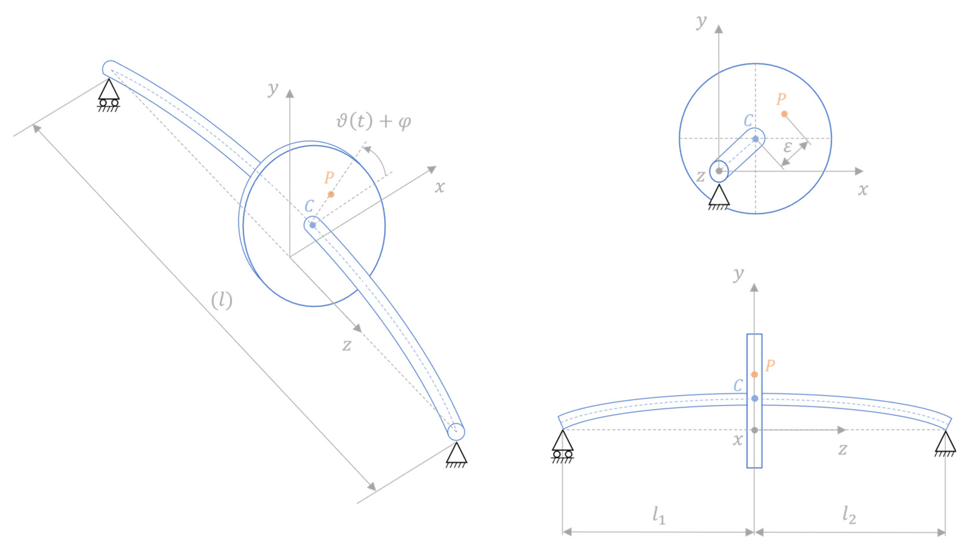
The PINN approach described in the previous Section is here applied on a numerical case study of a rotating shaft system in which the dynamics is simulated with the use of an extended Jeffcott rotor model [33]. The system, illustrated in Figure 2, consists of a

1 m

long rotating shaft (i.e.,

l = 1 m

) made of aluminium (Young’s modulus

E

set to

70000 M P a

, and density

ρ

equal to

2700 \frac{k g}{m^{3}}

) and supported at both ends. It has a circular cross section with a diameter of

20 m m

, and it incorporates a disk (representing, for instance, a flywheel, fan, turbine, gear, etc.) that is mounted at distances

l_{1}

and

l_{2}

from the respective supports. The shaft rotates at a velocity

Ω = \frac{d ϑ (t)}{d t}

, in which

ϑ (t)

denotes the angle defined with respect to the

x

axis of the right-handed

x y z

reference frame which is fixed in space. In this reference frame, the disk lies within the

x y

plane, and the

z

axis is aligned with the line connecting the two supports. Without any loss of generality, the disk is here considered to be positioned at the midpoint of the shaft, i.e.,

l_{1} = l_{2} = l / 2

. Moreover, the disk centre of mass

P

is displaced from the axis of rotation, whose trace in the disk plane is identified with the point

C

, generating a static unbalance defined by the distance

ε

and the angle

φ = ϑ (0)

. This unbalance causes the point

C

to displace from the line joining the supports leading the shaft to whirl around it.

The numerical model used to compute the rotor dynamics consists of a system of two second-order ODEs with a state vector of two components (making reference to Section 2,

n = 2

and

p = 2

, respectively), as reported in Eq. (6) and Eq. (7):

[\begin{matrix} m & 0 \\ 0 & m \end{matrix}] \{\begin{matrix} {\ddot{x}}_{c} \\ {\ddot{y}}_{c} \end{matrix}\} + [\begin{matrix} c_{n} + c_{r} & 0 \\ 0 & c_{n} + c_{r} \end{matrix}] \{\begin{matrix} {\dot{x}}_{c} \\ {\dot{y}}_{c} \end{matrix}\} + [\begin{matrix} k_{x} & {Ω \cdot c}_{r} \\ - Ω {\cdot c}_{r} & k_{y} \end{matrix}] \{\begin{matrix} x_{c} \\ y_{c} \end{matrix}\} = \{\begin{matrix} f_{x} \\ f_{y} \end{matrix}\}

(6)

\{\begin{matrix} f_{x} \\ f_{y} \end{matrix}\} = \{\begin{matrix} m_{d} \cdot ε \cdot (Ω^{2} \cdot c o s (Ω \cdot t + φ) + \dot{Ω} \cdot s i n (Ω \cdot t + φ)) \\ m_{d} \cdot ε \cdot (Ω^{2} \cdot s i n (Ω \cdot t + φ) - \dot{Ω} \cdot c o s (Ω \cdot t + φ)) - m \cdot g \end{matrix}\}

(7)

where

x_{c}

and

y_{c}

denote the

x

and

y

coordinates of the point

C

, respectively, and represent the components of the state vector (i.e.,

u = [x_{c}, y_{c}]

);

c_{n}

and

c_{r}

are the equivalent viscous damping terms of the stationary and rotating parts of the system, respectively;

m

represents the summation of the disk mass

m_{d}

and the shaft equivalent mass at the disk location

m_{s}^{e}

;

g

indicates the gravity acceleration;

k_{x}

and

k_{y}

are the system stiffnesses along the

x

and

y

axes, respectively, that are assumed to coincide with the axes of the ellipse of elasticity, i.e., the principal axes of elasticity of the supporting structure. Notably, the rotating damping

c_{r}

is here considered to be coincident to the contribution given by the shaft material properties, thus neglecting any potential additional term, and it is computed exploiting the approximation of a linear system [33], i.e.,

c_{r} = 2 ξ_{r} \sqrt{k_{s} \cdot m_{s}}

. Here,

ξ_{r}

denotes the rotational damping coefficient, that is assumed to be

0.001

m_{s}

represents the mass of the shaft, while

k_{s} = \frac{48 \cdot E \cdot I}{l^{3}}

denotes the shaft flexural stiffness, with

I

indicating the moment of inertia of the shaft cross section. The disk mass

m_{d}

is considered to be equal to

2 k g

, while the shaft equivalent mass at the disk location

m_{s}^{e}

is computed as

m_{s}^{e} = \frac{k_{s} \cdot δ}{g}

, in which

δ = \frac{5 \cdot m_{s} \cdot g \cdot l^{3}}{384 \cdot E \cdot I}

denotes the static displacement of the shaft at the disk location due to the shaft weight. The stiffnesses

k_{x}

and

k_{y}

are the combination of the shaft stiffness

k_{s}

and those of the supports

k_{b}^{x}

and

k_{b}^{y}

along the

x

and

y

axes, respectively. That is,

\frac{1}{k_{x}} = \frac{1}{k_{s}} + \frac{1}{k_{b}^{x}}

and

\frac{1}{k_{y}} = \frac{1}{k_{s}} + \frac{1}{k_{b}^{y}}

. However, determining the stiffness values of the supports can be challenging for different reasons, e.g., when they have complex geometries and interactions, due to misalignments or imperfections in installation, when the support materials is not well-defined or uniform, and they can change due to degradation over time [34]. A similar reasoning applies for the non-rotating damping and for the static unbalance. Hence, in this work

ε

φ

c_{n}

k_{x}

and

k_{y}

represent the components of the parameter vector

λ

, and their values are estimated through a PINN. Such parameters are selected because tracking their value is essential for maintaining the performance, reliability, and safety of rotating machinery.

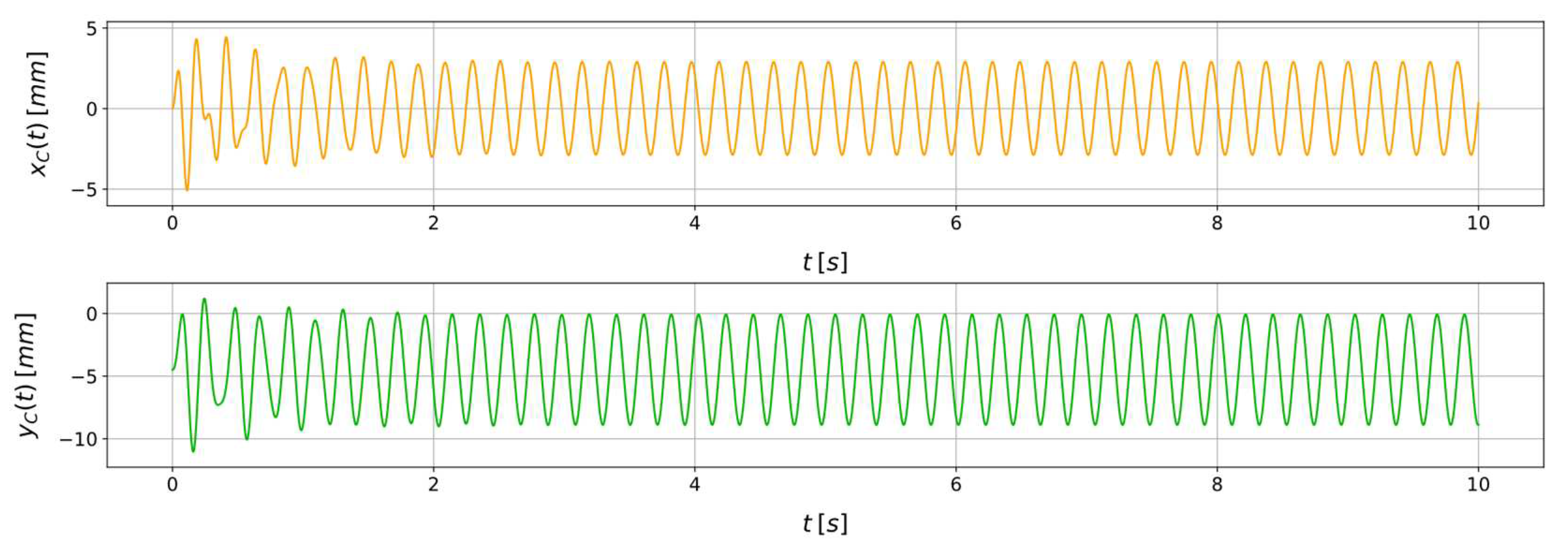
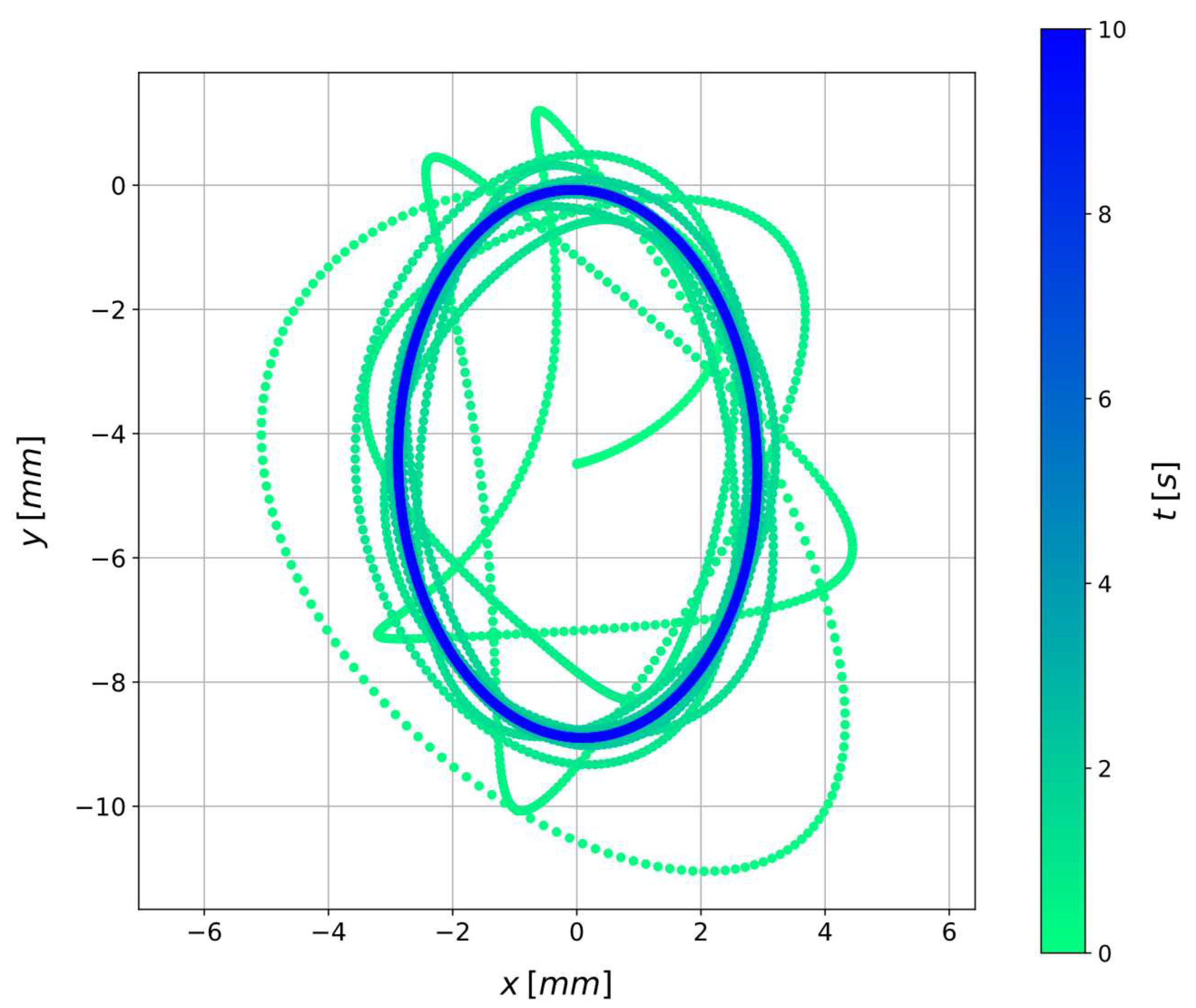
Figure 3 shows the model responses

x_{c}

and

y_{c}

obtained by solving Eq. (6) and Eq. (7) with a Runge-Kutta 4/5 integration method [35] in the time range

[0,10] s

. In the simulated scenario a constant rotational speed of

Ω = 30 \frac{r a d}{s}

is imposed, and

k_{x} = 7.76 \frac{N}{m m}

k_{y} = 6.71 \frac{N}{m m}

c_{n} = 7.0 \cdot 10^{- 3} \frac{N \cdot s}{m m}

ε = 8 m m

φ = 10 d e g

. No artificial noise is added. Figure 4 shows the scatter plot of the position of the disk centre

C

in the

x y

plane over time.

3.2. System state characterization through physics-informed neural networks

A PINN is then exploited to estimate the unknown parameters of the analysed rotating shaft system, i.e., to estimate the parameter vector

λ = [ε, φ, c_{n}, k_{x}, k_{y}]

. Notably, the employed NN architecture consists of 1 input neuron that takes in the generic time instant

t

, 1 hidden layer made of 200 neurons, and 2 output neurons to predict the values of

x_{C}

and

y_{C}

. Moreover, the hyperbolic tangent

t a n h

activation function [36] is used in the hidden layer, while the output layer embeds a linear activation function. The true system responses

x_{C}

and

y_{C}

required for training the PINN are numerically obtained with the Runge-Kutta 4/5 integration method in the time range

[0,1] s

(i.e.,

t_{0} = 0 s

and

t_{f} = 1 s

). Within this range, the true solution is sampled with a sampling frequency of

10 k H z

, which means that 10001 equally spaced points are considered in time. The same time instants are also considered for building the vector

t_{e}

that is used for training (i.e.,

N_{f} = 10001

). It is worth noting that various sampling frequency values were examined in this study. Specifically, the investigation covered a sampling frequency range of

[1, 10] k H z

with increments of

3 k H z

. Due to the similarity in outcomes from the analysis, these results are omitted here for the sake of conciseness.

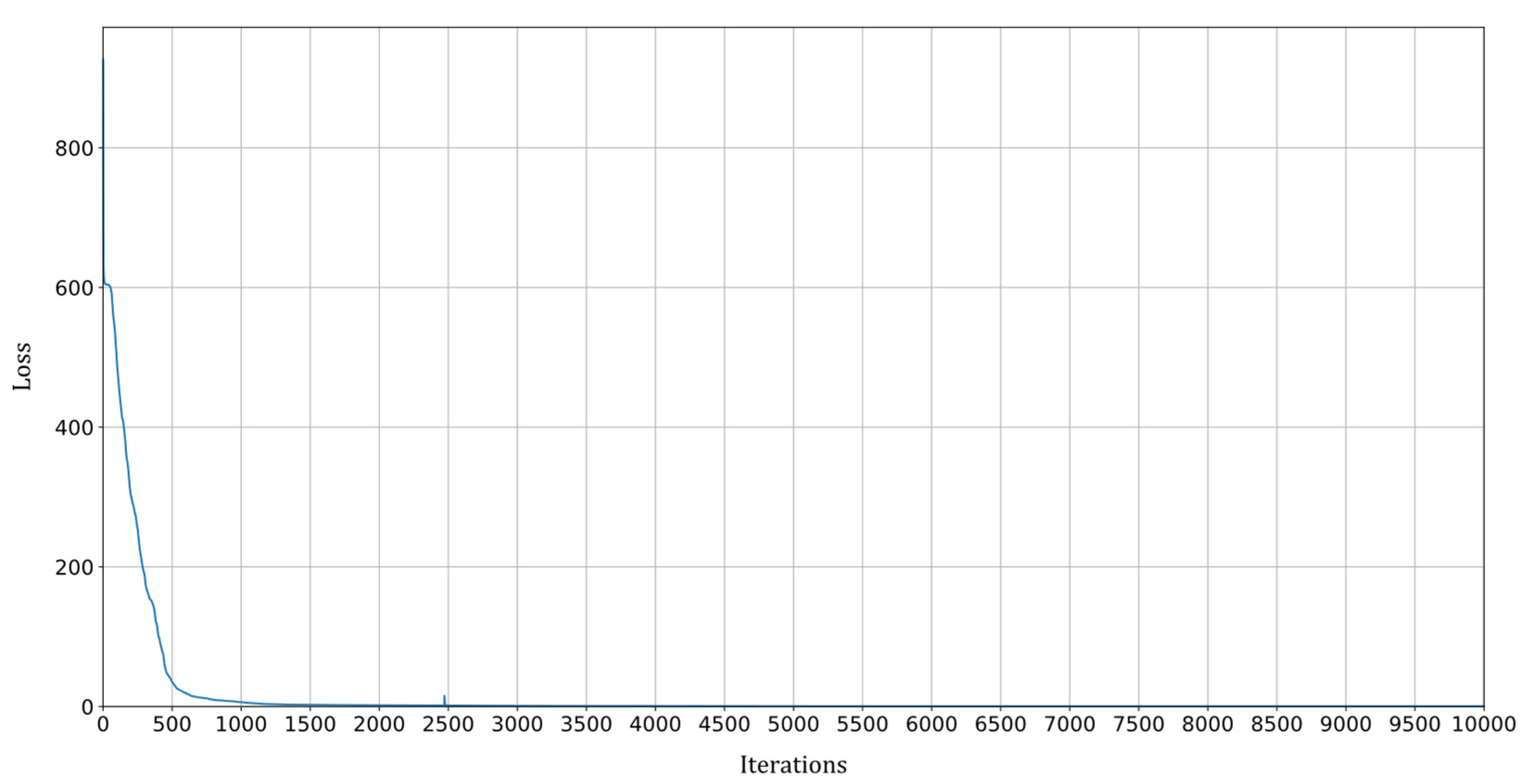
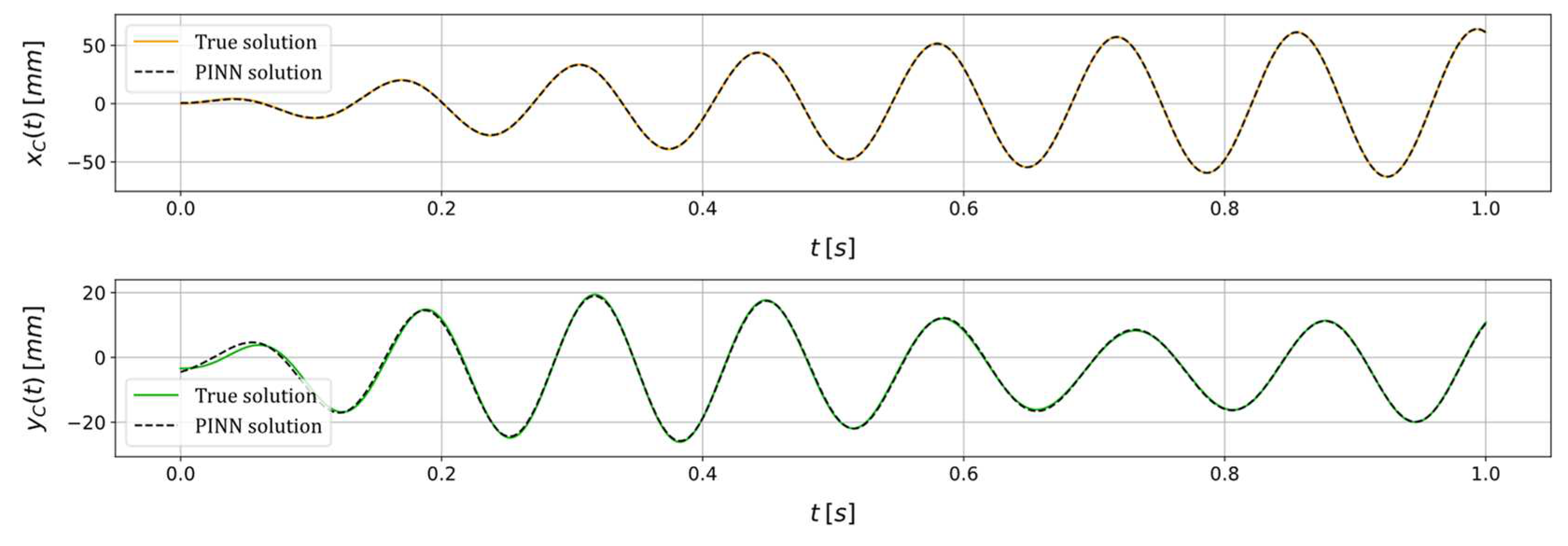
A representative scenario is examined to assess the efficacy of the proposed methodology. The scenario involves the imposition of a constant rotational speed of

Ω = 45 \frac{r a d}{s}

, alongside the following unknown parameters:

ε = 8.00 m m

φ = 10.00 d e g

c_{n} = 7.00 \cdot 10^{- 3} \frac{N \cdot s}{m m}

k_{x} = 5.53 \frac{N}{m m}

k_{y} = 7.25 \frac{N}{m m}

. No artificial noise is added to the system responses. The PINN is trained on an AMD Ryzen 9 5900HX 3.30

G H z

processor using a limited-memory Broyden–Fletcher–Goldfarb–Shanno (LBFGS) optimization algorithm [37] with a learning rate of

η = 0.01

, and encompassing

10000

training iterations. Moreover, the arbitrary initial guess set for the unknown parameters are

ε = 0.00 m m

φ = 0.00 d e g

c_{n} = 0.001 \cdot 10^{- 3} \frac{N \cdot s}{m m}

k_{x} = 1.00 \frac{N}{m m}

k_{y} = 2.00 \frac{N}{m m}

. The training process, as depicted in Figure 5, illustrates the progressive reduction of the training loss as the number of iterations increases. Instead, Figure 6 shows how the trained PINN is able to fit the available data to estimate the unknown parameters, showing a comparison between the true solution and the one obtained with the PINN. The outcome reveals that the approximation of the state vector offered by the PINN closely aligns with the actual vector, showcasing marginal disparities primarily observed in the state variable

y_{C}

during the initial time instants. Finally, the true value and the correspondent PINN estimation for all the system unknown parameters is shown in Table 1. What emerges is that all the parameters are estimated by the PINN with a remarkable accuracy, presenting the best performance in identifying the system stiffness values

k_{x}

and

k_{y}

, where the relative error in the estimation remains below

0.70 %

. Notably, among the parameters under estimation, the angle

φ

of the static unbalance and the non-rotating damping

c_{n}

prove to be the most challenging. This observation finds potential justification in the relatively subdued impact these parameters exert on the state variables compared to their counterparts. Nevertheless, even in these instances, the relative error remains constrained within

5.80 %

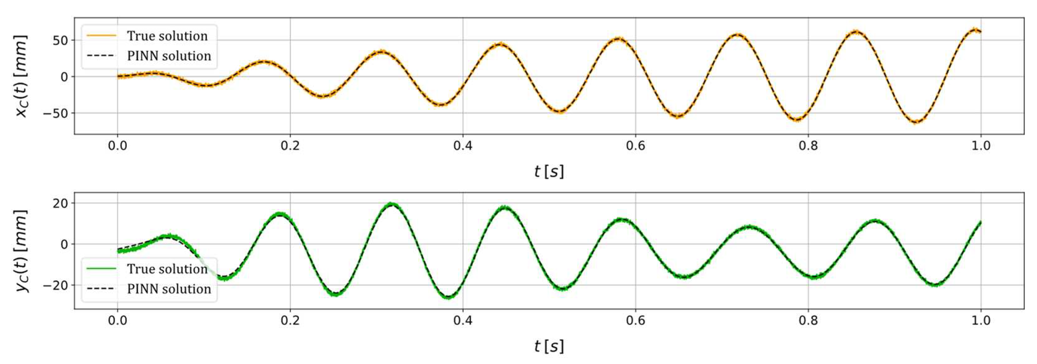
In order to assess the robustness of the PINN to external influences affecting input data (e.g., measurement noise, environmental vibrations, etc.), the same scenario is revisited while maintaining consistent training process conditions (i.e., algorithm used, learning rate, initial parameters guess, etc.). In this context, the input variables

x_{C}

and

y_{C}

, employed for the estimation of system parameters, are subjected to a perturbation through the introduction of supplementary numerical noise with a signal-to-noise ratio (

S N R

) of

40 d B

. The data fitting performed by the PINN and the parameters estimation are reported in Figure 7 and Table 2, respectively. The outcomes demonstrate that the PINN continues to function as a dependable tool for characterizing the health state of the system, even when confronted with external disturbances within the input data. Notably, no indications of diminished algorithm performance are discernible, with all parameter estimations retaining a relative error of less than

6.00 %

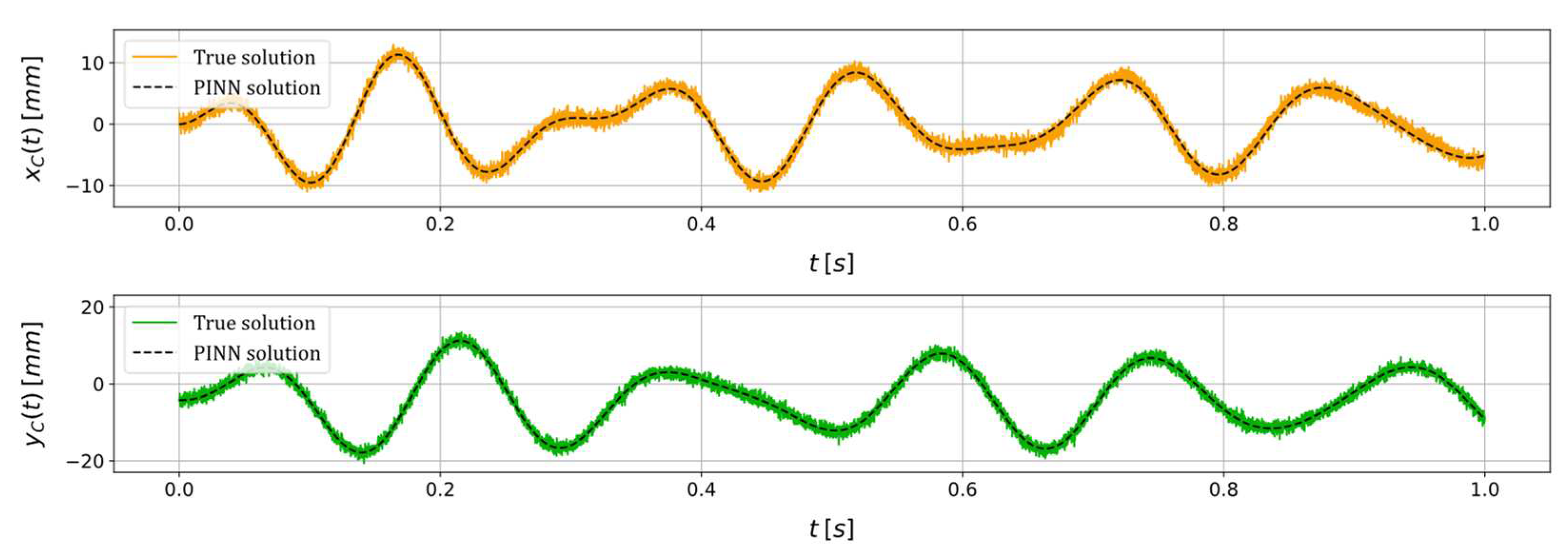
Lastly, an additional example is presented below to assess the estimation capabilities of the PINN when fed with data pertaining to a scenario marked by distinct imposed conditions and health states. The scenario encompasses the application of a constant rotational speed of

Ω = 35 \frac{r a d}{s}

, accompanied by the following unknown parameters:

ε = 12.00 m m

φ = 20.00 d e g

c_{n} = 5.00 \cdot 10^{- 3} \frac{N \cdot s}{m m}

k_{x} = 7.76 \frac{N}{m m}

k_{y} = 6.14 \frac{N}{m m}

. Moreover, an artificial noise with an

S N R

30 d B

is added to the input data, and the same training conditions of the previous scenarios are kept. The true and PINN solutions of the state variables

x_{C}

and

y_{C}

are reported in Figure 8, and the estimation of the unknown parameters is shown in Table 3. The PINN approximation of the state variables

x_{C}

and

y_{C}

appears to closely match the true solution. That is, the PINN manages to smooth out all the perturbances introduced by the added numerical noise, thus acting as a filter. The unknown parameters are satisfactorily estimated even in this scenario. The lowest relative estimation error characterises the system stiffnesses

k_{x}

and

k_{y}

, i.e.,

0.52 %

and

0.16 %

, respectively, while the non-rotating damping

c_{n}

is identified with a

9.80 %

error, which may be mainly related to the considerable amount of noise added.

4. Discussion

The paper has introduced a novel approach employing PINNs for estimating unknown parameters characterizing the health state of rotating shaft systems. The investigation has focused on a realistic numerical case study involving an extended Jeffcott rotor model, which has incorporated damping effects and anisotropic supports. The parameters considered have encompassed the radial and angular position of static unbalance caused by a shaft-mounted disk, stiffness values along the principal axes of elasticity, and the non-rotating damping coefficient. The estimation has relied exclusively on displacement signals from the disk centre, and various scenarios, incorporating different constant rotational speeds, have been thoroughly examined. Results have revealed the implemented PINN accuracy in estimating these parameters, demonstrating minimal relative errors even in the presence of substantial data noise. Beyond optimizing machinery performance and enhancing efficiency and reliability, the proposed estimation method has facilitated predictive maintenance by early fault identification.

Future works may explore (i) extending the approach to more complex rotor systems, (ii) experimental validation, and (iii) conducting comparative studies with other cutting-edge methods and machine learning approaches for parameter estimation in rotating systems.

Author Contributions

Conceptualization, M. P.; methodology, M. P.; software, M. P.; validation, M. P.; formal analysis, M. P.; investigation, M. P.; resources, M. P.; data curation, M. P.; writing—original draft preparation, M. P.; writing—review and editing, M. P. and L. L.; visualization, M. P.; supervision, F. C.; project administration, M. P., L. L. and F. C.; funding acquisition, M. G. and F. C. All authors have read and agreed to the published version of the manuscript.

Funding

This research received no external funding.

Data Availability Statement

The data presented in this study are available on request from the corresponding author.

Conflicts of Interest

The authors declare no conflict of interest.

References

Tandon, N.; Parey, A. Condition Monitoring of Rotary Machines. 2006, 109–136. [CrossRef]
Jeong, H.; Park, S.; Woo, S.; Lee, S. Rotating Machinery Diagnostics Using Deep Learning on Orbit Plot Images. Procedia Manuf. 2016, 5, 1107–1118. [Google Scholar] [CrossRef]
Tiboni, M.; Remino, C.; Bussola, R.; Amici, C. A Review on Vibration-Based Condition Monitoring of Rotating Machinery. Appl. Sci. 2022, Vol. 12, Page 972 2022, 12, 972. [Google Scholar] [CrossRef]
Silva, D.; Mendes, J.C.; Pereira, A.B.; Gégot, F.; Alves, L.N. Measuring Torque and Temperature in a Rotating Shaft Using Commercial SAW Sensors. Sensors 2017, Vol. 17, Page 1547 2017, 17, 1547. [Google Scholar] [CrossRef]
Nandi, S.; Toliyat, H.A.; Li, X. Condition Monitoring and Fault Diagnosis of Electrical Motors - A Review. IEEE Trans. Energy Convers. 2005, 20, 719–729. [Google Scholar] [CrossRef]
Farrar, C.R.; Worden, K. An Introduction to Structural Health Monitoring. Philos. Trans. R. Soc. A Math. Phys. Eng. Sci. 2006, 365, 303–315. [Google Scholar] [CrossRef]
Hameed, Z.; Hong, Y.S.; Cho, Y.M.; Ahn, S.H.; Song, C.K. Condition Monitoring and Fault Detection of Wind Turbines and Related Algorithms: A Review. Renew. Sustain. Energy Rev. 2009, 13, 1–39. [Google Scholar] [CrossRef]
Zhou, H.; Huang, X.; Wen, G.; Lei, Z.; Dong, S.; Zhang, P.; Chen, X. Construction of Health Indicators for Condition Monitoring of Rotating Machinery: A Review of the Research. Expert Syst. Appl. 2022, 203, 117297. [Google Scholar] [CrossRef]
Bogue, R. Sensors for Condition Monitoring: A Review of Technologies and Applications. Sens. Rev. 2013, 33, 295–299. [Google Scholar] [CrossRef]
Sohn, H. Effects of Environmental and Operational Variability on Structural Health Monitoring. Philos. Trans. R. Soc. A Math. Phys. Eng. Sci. 2006, 365, 539–560. [Google Scholar] [CrossRef] [PubMed]
Parziale, M.; Lomazzi, L.; Giglio, M.; Cadini, F. Vibration-Based Structural Health Monitoring Exploiting a Combination of Convolutional Neural Networks and Autoencoders for Temperature Effects Neutralization. Struct. Control Heal. Monit. 2022, 29, e3076. [Google Scholar] [CrossRef]
Zhao, R.; Yan, R.; Chen, Z.; Mao, K.; Wang, P.; Gao, R.X. Deep Learning and Its Applications to Machine Health Monitoring. Mech. Syst. Signal Process. 2019, 115, 213–237. [Google Scholar] [CrossRef]
Fu, J.; Chu, J.; Guo, P.; Chen, Z. Condition Monitoring of Wind Turbine Gearbox Bearing Based on Deep Learning Model. IEEE Access 2019, 7, 57078–57087. [Google Scholar] [CrossRef]
O’Shea, K.; Nash, R. An Introduction to Convolutional Neural Networks. Int. J. Res. Appl. Sci. Eng. Technol. 2015, 10, 943–947. [Google Scholar] [CrossRef]
Schmidt, R.M. Recurrent Neural Networks (RNNs): A Gentle Introduction and Overview. 2019.
Souza, R.M.; Nascimento, E.G.S.; Miranda, U.A.; Silva, W.J.D.; Lepikson, H.A. Deep Learning for Diagnosis and Classification of Faults in Industrial Rotating Machinery. Comput. Ind. Eng. 2021, 153, 107060. [Google Scholar] [CrossRef]
Wisal, M.; Oh, K.Y. A New Deep Learning Framework for Imbalance Detection of a Rotating Shaft. Sensors 2023, Vol. 23, Page 7141 2023, 23, 7141. [Google Scholar] [CrossRef]
He, K.; Zhang, X.; Ren, S.; Sun, J. Deep Residual Learning for Image Recognition 2016, 770–778.
Dosilovic, F.K.; Brcic, M.; Hlupic, N. Explainable Artificial Intelligence: A Survey. 2018 41st Int. Conv. Inf. Commun. Technol. Electron. Microelectron. MIPRO 2018 - Proc. 2018, 210–215. [CrossRef]
Lomazzi, L.; Fabiano, S.; Parziale, M.; Giglio, M.; Cadini, F. On the Explainability of Convolutional Neural Networks Processing Ultrasonic Guided Waves for Damage Diagnosis. Mech. Syst. Signal Process. 2023, 183, 109642. [Google Scholar] [CrossRef]
Parziale, M.; Lomazzi, L.; Giglio, M.; Cadini, F. Transmissibility Functions-Based Structural Damage Assessment with the Use of Explainable Convolutional Neural Networks. 2023, 540–549. [CrossRef]
Parziale, M.; Henrique Silva, P.; Giglio, M.; Cadini, F. Explainability of Convolutional Neural Networks for Damage Diagnosis Using Transmissibility Functions. [CrossRef]
Raissi, M.; Perdikaris, P.; Karniadakis, G.E. Physics-Informed Neural Networks: A Deep Learning Framework for Solving Forward and Inverse Problems Involving Nonlinear Partial Differential Equations. J. Comput. Phys. 2019, 378, 686–707. [Google Scholar] [CrossRef]
Raissi, M.; Perdikaris, P.; Karniadakis, G.E. Physics Informed Deep Learning (Part I): Data-Driven Solutions of Nonlinear Partial Differential Equations. 2017.
Haghighat, E.; Raissi, M.; Moure, A.; Gomez, H.; Juanes, R. A Physics-Informed Deep Learning Framework for Inversion and Surrogate Modeling in Solid Mechanics. Comput. Methods Appl. Mech. Eng. 2021, 379, 113741. [Google Scholar] [CrossRef]
Shen, S.; Lu, H.; Sadoughi, M.; Hu, C.; Nemani, V.; Thelen, A.; Webster, K.; Darr, M.; Sidon, J.; Kenny, S. A Physics-Informed Deep Learning Approach for Bearing Fault Detection. Eng. Appl. Artif. Intell. 2021, 103, 104295. [Google Scholar] [CrossRef]
Garpelli, L.N.; Alves, D.S.; Cavalca, K.L.; de Castro, H.F. Physics-Guided Neural Networks Applied in Rotor Unbalance Problems. https://doi.org/10.1177/14759217231163081 2023. [CrossRef]
Deng, W.; Nguyen, K.T.P.; Medjaher, K.; Gogu, C.; Morio, J. Rotor Dynamics Informed Deep Learning for Detection, Identification, and Localization of Shaft Crack and Unbalance Defects. Adv. Eng. Informatics 2023, 58, 102128. [Google Scholar] [CrossRef]
Cybenko, G. Approximation by Superpositions of a Sigmoidal Function. Math. Control. Signals, Syst. 1989, 2, 303–314. [Google Scholar] [CrossRef]
Wang, S.-C. Artificial Neural Network. Interdiscip. Comput. Java Program. 2003, 81–100. [CrossRef]
Margossian, C.C.; Charles Margossian, C.C. A Review of Automatic Differentiation and Its Efficient Implementation. Wiley Interdiscip. Rev. Data Min. Knowl. Discov. 2019, 9, e1305. [Google Scholar] [CrossRef]
Al Seyab, R.K.; Cao, Y. Nonlinear System Identification for Predictive Control Using Continuous Time Recurrent Neural Networks and Automatic Differentiation. J. Process Control 2008, 18, 568–581. [Google Scholar] [CrossRef]
Genta, G.; Keith, R.H. Vibration Dynamics and Control. Noise Control Eng. J. 2009, 57, 156. [Google Scholar] [CrossRef]
Cerrada, M.; Sánchez, R.V.; Li, C.; Pacheco, F.; Cabrera, D.; Valente de Oliveira, J.; Vásquez, R.E. A Review on Data-Driven Fault Severity Assessment in Rolling Bearings. Mech. Syst. Signal Process. 2018, 99, 169–196. [Google Scholar] [CrossRef]
Bogacki, P.; Shampine, L.F. An Efficient Runge-Kutta (4,5) Pair. Comput. Math. with Appl. 1996, 32, 15–28. [Google Scholar] [CrossRef]
Rumelhart, D.E.; Hinton, G.E.; Williams, R.J. Learning Representations by Back-Propagating Errors. Nat. 1986 3236088 1986, 323, 533–536. [Google Scholar] [CrossRef]
Liu, D.C.; Nocedal, J. On the Limited Memory BFGS Method for Large Scale Optimization. Math. Program. 1989, 45, 503–528. [Google Scholar] [CrossRef]

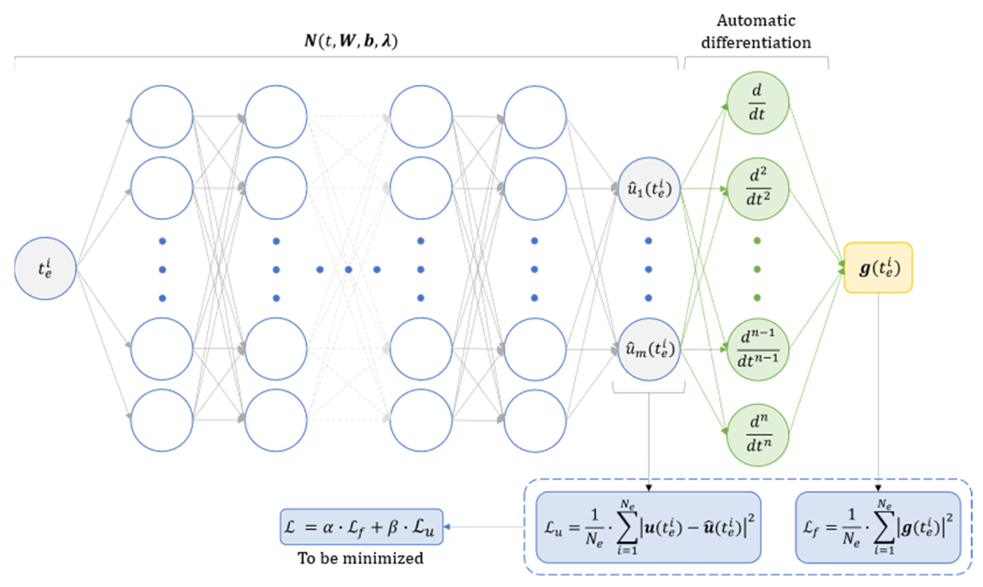
Figure 1. Scheme showing how a physics-informed neural network is trained to estimate the parameters vector

λ

of a system described by ODEs.

Figure 1. Scheme showing how a physics-informed neural network is trained to estimate the parameters vector

λ

of a system described by ODEs.

Figure 1. Scheme of the considered rotating shaft system with highlighted the disk geometrical centre (point

C

) and static unbalance (point

P

Figure 1. Scheme of the considered rotating shaft system with highlighted the disk geometrical centre (point

C

) and static unbalance (point

P

Figure 3. Example of the model responses

x_{C}

and

y_{C}

in a representative scenario with

Ω = 30 \frac{r a d}{s}

ε = 8.00 m m

φ = 10.00 d e g

c_{n} = 7.00 \cdot 10^{- 3} \frac{N \cdot s}{m m}

k_{x} = 7.76 \frac{N}{m m}

, and

k_{y} = 6.71 \frac{N}{m m}

Figure 3. Example of the model responses

x_{C}

and

y_{C}

in a representative scenario with

Ω = 30 \frac{r a d}{s}

ε = 8.00 m m

φ = 10.00 d e g

c_{n} = 7.00 \cdot 10^{- 3} \frac{N \cdot s}{m m}

k_{x} = 7.76 \frac{N}{m m}

, and

k_{y} = 6.71 \frac{N}{m m}

Figure 2. Visualization in the

x - y

plane of the disk centre position (

x_{C}, y_{C}

) over time

t

for a scenario in which a constant rotational speed of

Ω = 30 \frac{r a d}{s}

is imposed and where

ε = 8.00 m m

φ = 10.00 d e g

c_{n} = 7.00 \cdot 10^{- 3} \frac{N \cdot s}{m m}

k_{x} = 7.76 \frac{N}{m m}

k_{y} = 6.71 \frac{N}{m m}

, without adding artificial noise.

Figure 2. Visualization in the

x - y

plane of the disk centre position (

x_{C}, y_{C}

) over time

t

for a scenario in which a constant rotational speed of

Ω = 30 \frac{r a d}{s}

is imposed and where

ε = 8.00 m m

φ = 10.00 d e g

c_{n} = 7.00 \cdot 10^{- 3} \frac{N \cdot s}{m m}

k_{x} = 7.76 \frac{N}{m m}

k_{y} = 6.71 \frac{N}{m m}

, without adding artificial noise.

Figure 3. PINN training loss over the training iterations for a scenario in which a constant rotational speed of

Ω = 45 \frac{r a d}{s}

is imposed and where

ε = 8.00 m m

φ = 10.00 d e g

c_{n} = 7.00 \cdot 10^{- 3} \frac{N \cdot s}{m m}

k_{x} = 5.53 \frac{N}{m m}

k_{y} = 7.25 \frac{N}{m m}

, without adding artificial noise.

Figure 3. PINN training loss over the training iterations for a scenario in which a constant rotational speed of

Ω = 45 \frac{r a d}{s}

is imposed and where

ε = 8.00 m m

φ = 10.00 d e g

c_{n} = 7.00 \cdot 10^{- 3} \frac{N \cdot s}{m m}

k_{x} = 5.53 \frac{N}{m m}

k_{y} = 7.25 \frac{N}{m m}

, without adding artificial noise.

Figure 4. True and PINN solutions of the state variables

x_{C}

and

y_{C}

for a scenario in which a constant rotational speed of

Ω = 45 \frac{r a d}{s}

is imposed and where

ε = 8.00 m m

φ = 10.00 d e g

c_{n} = 7.00 \cdot 10^{- 3} \frac{N \cdot s}{m m}

k_{x} = 5.53 \frac{N}{m m}

k_{y} = 7.25 \frac{N}{m m}

, without adding artificial noise.

Figure 4. True and PINN solutions of the state variables

x_{C}

and

y_{C}

for a scenario in which a constant rotational speed of

Ω = 45 \frac{r a d}{s}

is imposed and where

ε = 8.00 m m

φ = 10.00 d e g

c_{n} = 7.00 \cdot 10^{- 3} \frac{N \cdot s}{m m}

k_{x} = 5.53 \frac{N}{m m}

k_{y} = 7.25 \frac{N}{m m}

, without adding artificial noise.

Figure 5. True and PINN solutions of the state variables

x_{C}

and

y_{C}

for a scenario in which a constant rotational speed of

Ω = 45 \frac{r a d}{s}

is imposed and where

ε = 8.00 m m

φ = 10.00 d e g

c_{n} = 7.00 \cdot 10^{- 3} \frac{N \cdot s}{m m}

k_{x} = 5.53 \frac{N}{m m}

k_{y} = 7.25 \frac{N}{m m}

, adding an artificial noise with a

S N R = 40 d B

Figure 5. True and PINN solutions of the state variables

x_{C}

and

y_{C}

for a scenario in which a constant rotational speed of

Ω = 45 \frac{r a d}{s}

is imposed and where

ε = 8.00 m m

φ = 10.00 d e g

c_{n} = 7.00 \cdot 10^{- 3} \frac{N \cdot s}{m m}

k_{x} = 5.53 \frac{N}{m m}

k_{y} = 7.25 \frac{N}{m m}

, adding an artificial noise with a

S N R = 40 d B

Figure 6. True and PINN solutions of the state variables

x_{C}

and

y_{C}

for a scenario in which a constant rotational speed of

Ω = 35 \frac{r a d}{s}

is imposed and where

ε = 12.00 m m

φ = 20.00 d e g

c_{n} = 5.00 \cdot 10^{- 3} \frac{N \cdot s}{m m}

k_{x} = 7.76 \frac{N}{m m}

k_{y} = 6.14 \frac{N}{m m}

, adding an artificial noise with a

S N R = 30 d B

Figure 6. True and PINN solutions of the state variables

x_{C}

and

y_{C}

for a scenario in which a constant rotational speed of

Ω = 35 \frac{r a d}{s}

is imposed and where

ε = 12.00 m m

φ = 20.00 d e g

c_{n} = 5.00 \cdot 10^{- 3} \frac{N \cdot s}{m m}

k_{x} = 7.76 \frac{N}{m m}

k_{y} = 6.14 \frac{N}{m m}

, adding an artificial noise with a

S N R = 30 d B

Table 1. True value and the correspondent PINN estimation for all the system unknown parameters related to a scenario in which a constant rotational speed of

Ω = 45 \frac{r a d}{s}

is imposed; no noise added to the processed system responses.

Table 1. True value and the correspondent PINN estimation for all the system unknown parameters related to a scenario in which a constant rotational speed of

Ω = 45 \frac{r a d}{s}

is imposed; no noise added to the processed system responses.

Unknown parameter	True value	PINN estimation	Relative error (%)
$ε$ $[m m]$	$8.00$	$7.87$	$1.63$
$φ$ $[d e g]$	$10.00$	$9.42$	$5.80$
$c_{n}$ $[\frac{N \cdot s}{m m}]$	$7.00 \cdot 10^{- 3}$	$6.70 \cdot 10^{- 3}$	$4.29$
$k_{x}$ $[\frac{N}{m m}]$	$5.53$	$5.54$	$0.18$
$k_{y}$ $[\frac{N}{m m}]$	$7.25$	$7.20$	$0.69$

Table 2. True value and the correspondent PINN estimation for all the system unknown parameters related to a scenario in which a constant rotational speed of

Ω = 45 \frac{r a d}{s}

is imposed; noise added to the processed system responses with a

S N R = 40 d B

Table 2. True value and the correspondent PINN estimation for all the system unknown parameters related to a scenario in which a constant rotational speed of

Ω = 45 \frac{r a d}{s}

is imposed; noise added to the processed system responses with a

S N R = 40 d B

Unknown parameter	True value	PINN estimation	Relative error (%)
$ε$ $[m m]$	$8.00$	$7.93$	$0.88$
$φ$ $[d e g]$	$10.00$	$9.42$	$5.80$
$c_{n}$ $[\frac{N \cdot s}{m m}]$	$7.00 \cdot 10^{- 3}$	$6.80 \cdot 10^{- 3}$	$2.86$
$k_{x}$ $[\frac{N}{m m}]$	$5.53$	$5.54$	$0.18$
$k_{y}$ $[\frac{N}{m m}]$	$7.25$	$7.26$	$0.14$

Table 3. True value and the correspondent PINN estimation for all the system unknown parameters related to a scenario in which a constant rotational speed of

Ω = 35 \frac{r a d}{s}

is imposed; noise added to the processed system responses with a

S N R = 30 d B

Table 3. True value and the correspondent PINN estimation for all the system unknown parameters related to a scenario in which a constant rotational speed of

Ω = 35 \frac{r a d}{s}

is imposed; noise added to the processed system responses with a

S N R = 30 d B

Unknown parameter	True value	PINN estimation	Relative error (%)
$ε$ $[m m]$	$12.00$	$11.96$	$0.33$
$φ$ $[d e g]$	$20.00$	$21.17$	$5.85$
$c_{n}$ $[\frac{N \cdot s}{m m}]$	$5.00 \cdot 10^{- 3}$	$5.49 \cdot 10^{- 3}$	$9.80$
$k_{x}$ $[\frac{N}{m m}]$	$7.76$	$7.72$	$0.52$
$k_{y}$ $[\frac{N}{m m}]$	$6.14$	$6.13$	$0.16$

Disclaimer/Publisher’s Note: The statements, opinions and data contained in all publications are solely those of the individual author(s) and contributor(s) and not of MDPI and/or the editor(s). MDPI and/or the editor(s) disclaim responsibility for any injury to people or property resulting from any ideas, methods, instructions or products referred to in the content.

© 2023 by the authors. Licensee MDPI, Basel, Switzerland. This article is an open access article distributed under the terms and conditions of the Creative Commons Attribution (CC BY) license (http://creativecommons.org/licenses/by/4.0/).

Copyright: This open access article is published under a Creative Commons CC BY 4.0 license, which permit the free download, distribution, and reuse, provided that the author and preprint are cited in any reuse.

MDPI Initiatives

Important Links

Choose an area of interest and we will send you notifications of new preprints at your preferred frequency.

Disclaimer

Physics-Informed Neural Networks for the Condition Monitoring of Rotating Shafts

Abstract

1. Introduction

2. Methodology

3. Case study

3.1. Extended Jeffcott rotor with unknown system parameters

3.2. System state characterization through physics-informed neural networks

4. Discussion

Author Contributions

Funding

Data Availability Statement

Conflicts of Interest

References

MDPI Initiatives

Important Links

Subscribe