Fast Bimetallic Nanoalloy Quantification Method Using X-ray Fluorescence Spectroscopy for High-Throughput Experiments

Le Nguyen-Vu

doi:10.20944/preprints202311.1452.v1

Submitted:

22 November 2023

Posted:

23 November 2023

You are already at the latest version

Abstract

High-throughput research on bimetallic nanoparticles brought a vast overview of their characteristics and catalytic activities.¹ However, traditional bimetallic nano-allloy quantification methods serving catalyst preparations are not suitable for the fast and robust data output of high-throughput experiments. Hence, this work designed and validated a more fast, more neat, and reliable quantitative analysis using X-ray fluorescence spectroscopy for bimetallic nanoparticles synthesized by high-throughput setups. The results demonstrated this method to be accurate with high precision. Furthermore, the agreement to qualitative results from an energy-dispersive X-ray spectrometer equiped on a scanning electron microscope provided an option to quantify a bimetallic nano-alloy by just analyzing one of the two composing elements. Thus, this method is proved to be highly compatible with high-throughput experiments.

Keywords:

quantitative analysis

;

X-ray fluorescence spectroscopy

;

bimetallic nanoparticle

;

nanoparticle concentration

Subject:

Chemistry and Materials Science - Analytical Chemistry

I. Introduction

In ancient time, humans applied alloying to enhance the desired properties of metallic material. Using the same principle, bimetallic nanoparticles (NPs) was also designed in order to achieve unique properties that are distinctive from their mono-metallic counterparts, serving special purposes mostly in catalysis.^1–7 In order to understand their properties, conventional experimentalists deploy many analyses and experiments such as characterizations of optical and electrical properties and morphology, elemental analyses, and catalytic tests. Even though conventional experiments results in deep understanding and reliable data on a specific subject, these kind of experiment are redundant and inconsistent among researches. These drawbacks bring ambiguities and misunderstanding information in a research area. To overcome these issues, we applied a series of high-throughput (HTP) experiments in order to construct the “Library of Bimetallic Three-way Catalyst” to portray a comprehensive picture of bimetallic nanoparticles in three-way catalysts.¹

The biggest challenge in our previous work was the quantification of bimetallic NPs solutions in order to control the amount of NPs loading on support materials. Conventional metal quantification methods involving instruments such as atomic absorption spectroscopy (AAS), atomic emission spectroscopy (AES), and mass spectroscopy (MS), require a lot of consuming resource and complicated procedures. Furthermore, they are destructive and may demand a large sample size for sample digestion. Thus, these methods are not compatible with our HTP experiments, which generate massive amounts of data in an extremely fast manner. One non-destructive method was reported by Haidi D. F. et al. using an energy-dispersive X-ray fluorescence (EDXRF) instrument. Their work showed that the signal from metal ions such as Pt²⁺, Rh²⁺, and Pd²⁺ are identical to metal state forms (Pt⁰, Rh⁰, and Pd⁰) regardless of their particle sizes.⁸ However, their method was subjected only to their mono-metallic particles synthesized using conventional experiments and the standard solution for their quatification analyses are more readily available than for bimetallic species in HTP syntheses. Moreover, their procedure involved solvent-removing stages that are very difficult to be done sometime in bimetallic cases. Hence, we design a more simple quantification method that is greatly compatible with HTP bimetallic alloy syntheses using XRF with minor sample preparations without removing the original sample solvent yet still resembling the sample matrix to the respective standard solution matrix. The method was validated based on the suggestions of ISO standards (ISO 170025:2017 and ISO 5725:1994 part 1 and 2) and other references. The qualitative results of an energy-dispersive X-ray spectrometer (EDS) and the quantitative results of XRF agreed with each other and this finding allowed users to quantify bimetallic alloy easily and quickly by analyzing just one of the constituent elements. Therefore, this method was proved to be fast and highly compatible with HTP experiments.

II. Experimental section

Material

Hydrogen hexachloroplatinate (IV) hexahydrate (H₂PtCl₆-6H₂O, ≥ 98.5 %), potassium tetrachloropalladate (II) (K₂PdCl₄, 99 %), rhodium (III) chloride trihydrate (RhCl₃-3H₂O, 99.5 %), triethylene glycol (99 %), and polyvinylpyrrolodine ((C₆H₉NO)_n, K30, average MW = 40000) were purchased from Wako. Palladium (II) chloride (PdCl₂, ≥ 99.9 %), ruthenium (III) chloride hydrate (RuCl₃-xH₂O, Ru 46.8 %), and iridium chloride hydrate (IrCl₃-xH₂O, Ir 54.6 %) were purchased from Sigma Aldrich. Hydrochloric acid (35.0 % ~ 37.0 %), acetone, hexane, and methanol of research grade are purchased from Kanto Chemical. DI water with an electrical resistance of 16 MΩ was employed.

Synthesis

This work using the same synthetic method as in the “Library of bimetallic three-way catalysts”.¹ In a recap, A mixture of 88 mg of polyvinylpyrrolidone (PVP) and 20 ml of triethylene glycol (TEG) were vigorously stirred under N₂ while being heated to 190 ^oC. Thereafter, 2.0 ml of an aqueous solution containing metal precursors (0.050 mmol per metal element) and 22 mg of PVP, was quickly introduced into the hot TEG-PVP mixture, forming a black solution. The black mixture was then kept for 30 min and slowly cooled to room temperature. The nano-products were extracted from the TEG solution by an acetone/hexane mixture (3/1 v/v), and centrifugation. Finally, the synthesized bimetallic nanoparticles were re-dispersed and stored in methanol before analyses.

Standard solutions and samples preparation

1000 mg/kg stock solutions of five elements, Pd, Pt, Rh, Ru, and Ir, were prepared by dissolving respectively PdCl₂, H₂PtCl₆-6H₂O, RhCl₃-3H₂O, RuCl₃-xH₂O and IrCl₃-xH₂O in a 5% hydrochloric aqueous matrix. Subsequently, a 100 mg/kg multi-element standard solution was prepared from the stock. For sample preparation, around 0,5 ml of nanoparticles solution was diluted from 10 to 100 times with DI water (16 MΩ). All dilutions and preparations were made gravimetrically using an analytical balance (Metter Toledo QD205DR, Max1 = 220 g, d1 = 0,1 mg, Max2 = 81 g, d2 = 0,01 mg).

Characterization and analysis

Transmission electron microscopic (TEM) images were taken on a Hitachi H-7100 electron microscope operated at 100kV. 200 particles were under a survey to determine the average particle size and the particle size distribution. Powder X-ray diffraction (XRD) data were recorded on a Rigaku SmartLab X-ray diffractometer employing a Cu-Kα radiation source. Elemental analysis was conducted using a scanning electron microscope equipped with an energy-dispersive X-ray spectrometer (SEM-EDS, TM3030 Plus Microscope). EDS signals were collected at nine different locations on a dried sample droplet and averaged to define the chemical composition.

The quantitative analyses were performed on an X-ray fluorescence spectrometer (XRF, PanAlytical Epsilon 3) equipped with an Ag X-ray tube, and a Cu filter having 500 μm thickness. The X-ray tube and generator have an operating specification under a potential range from 4 kV to 50 kV and a current range from 1 μA to 3000 μA, which provides the maximum power of 15W. XRF signal was recorded under ambient air with an acquisition time of 60 seconds. In each measurement, 3.0 ml of a standard solution or a sample solution was added into a sample cup (35 mm in dia.) supported by a 6 μm-thick PP film. Measurements were repeated three times for every sample and calibration point to determine the precision of the method.

III. Results and discussion

Synthesis

The successes in syntheses of PdPt, PdRh, PtRh, RhRu, PtRu and PtIr were reported in the “Library of bimetallic three-way catalyst”.¹ In Figure 1, bimetallic peaks located in between the monometallic peaks were clearly seen in the alloys of PdRh, PtRh, RhRu and, PtRu and indicated their successful syntheses according to Velgard’s law. For PdPt and PtIr, because of the similarity of the XRD peaks of the two elemental constituents, the homogeneities of the XRD peaks as well as of SEM-EDS results (Table 1) were taken into account to confirm their successful alloy formation.

TEM images in Figure 2 describe the well-uniform particle size distribution as well as the good dispersion of all six bimetallic combinations. Therefore, the homogeneities of the six bimetallic alloy solutions were assured and are suitable for the method validation.

Method validation

Subclause 7.2 of ISO 17025:2017 suggests all necessary parameters need to be checked for method validation.⁹ However, in this paper, only the five parameters defined below were majorly focused on due to the limitation of our laboratory’s resources. In addition, the definitions of them in this paper are a bit different than those in ISO 5725-1:1994.¹⁰ Hereby, to avoid unnecessary ambiguity, we will re-clarify their definition and describe the method of how to demonstrate them in this work before the validation discussion.

Definitions

Accuracy¹¹ or trueness¹⁰, measures the nearness to the truth.¹¹ This work demonstrated it by comparing results from two or more different analytical methods and expected to agree within their expected precision.

Precision shows how well replicate measurements agree with one another.¹¹ In this case, it was evaluated by calculating the repeatability and the Intermediate precision¹¹ (same laboratory, same instrument, same method but different operators and different time) of the method. Since it was inapplicable to perform reproducibility (different laboratory, different instrument, and different operator) evaluation, the intermediate precision was treated as Reproducibility and calculated using the formulas in subclause 7.4 of ISO 5725-2:1994.¹²

Linearity evaluates how well a calibration curve follows a straight line, which demonstrates the proportional relationship between the signal and the amount of analyte.¹¹

Lowest limit of detection (LoD) is the smallest quantity of analyte that is significantly different from the blank but not enough for accurate measurement.¹¹ Signal-to-noise ratio S/N = 3 for LoD.

Lowest limit of quantification (LoQ) is the smallest amount that can be measured with reasonable accuracy.¹¹ Signal-to-noise ratio S/N = 10 for LoQ.

The calibration curves in Table 2 were derived by using the method of least square in which the sum of squares of the vertical deviations between the data points and the line is minimized.

Calibration curve:

y = m x + b

, where y is the XRF signal, x is the concentration of analytes, m is the slope of the linear line.

Vertical deviation for the point (

x_{i}, y_{i}

) =

d_{i} = y_{i} - y = y_{i} - (m x + b)

The standard deviation of vertical deviation =

s_{y} = \sqrt{\frac{\sum (d_{i}^{2})}{n - 2}}

,where n is the number of data points

Thereby, the signal of detection limit was estimated to be equal

{b + 3 s}_{y}

,¹¹ hence the LoD =

\frac{{3 s}_{y}}{m}

, and LoQ =

\frac{{10 s}_{y}}{m}

Validation results

This method was extrapolated from the assumption that the matrix between the standard solution (5% HCl) and sample (DI water with a small amount of methanol and PVP) resembles. To test the hypothesis, a t-test for comparing two different sets of replicate measurements was performed. As can be seen in Table 2, the calculated t-value were all below the theoretical t-value, indicating that the sets of data from 5% HCl matrix and sample matrix agree each to other. These results prove that the two backgrounds of analyses are not significantly different.

In Table 1, the RSDs of the quantitative results are below 5,3%, which is the predicted standard deviation for repeatability at 100 ppm of mass fraction (see AOAC appendix F: SMPR Guidline),¹³ demonstrating that the method has extremely high repeatability. For evaluating reproducibility, the reproducibility variance¹² of PdRh results from two measurements six months away from each other. Table 3 reported the relative intermediate precision variance (

{R S D}_{R}^{}

) of 2,35% that is much lower than the predicted standard deviation, 8%, for reproducibility at 10^-4 of mass fraction,¹³ indicating the method to be highly reproducible. Overall, this quantitative method possessed relatively high precision.

Moreover, the square of correlation coefficients R² of all five calibration curves are all higher than 0.995,¹¹ which indicates good linearity (Table 4). In addition, Pt and Ir had slopes of 3,9548 and 2,6228, which are much higher than others, showing that these heavy elements have a higher sensitivity than of the lighter ones.

In Table 4, The LoDs of all five target elements are above 1 mg/kg which was rational since the published LoD from the instrument manufacturer is 1ppm (roughly 1mg/kg).¹⁴ Besides, the LoQ of all five elements is suitable for quantifying common nanoparticle solution synthesized in research laboratories. Thus, the XRF quantitative results in Table 1 are reliable.

To evaluate the accuracy, XRF quantitative results were converted to the molar ratio form. Hereafter, the molar ratio results from SEM-EDS and the XRF calibration method were taken under a paired t-Test for comparing individual differences by assuming that SEM-EDS results are more reliable since the uncertainty of SEM-EDS results were much more narrow than of XRF calibration method. In the matter of fact, SEM-EDS is a very straight-forward analysis without any redundant sample preparations that might interfere to the final results.

In Table 5, The calculated t was roughly 1,523, which is lower than the theoretical t value 2,571 at 95% confidence. Thus, there is more than 5% chance, the two sets of results lie within experimental error. Or in another word, the results from these two methods agreed to each other. This finding demonstrated that it is possible to quantify bimetallic alloy solution by just quantifying one of two elemental components in the alloy. Therefore, this interchangeability with SEM-EDS allows the XRF calibration method to be compatible with high-throughput (HTP) experiments, which generate a massive amount of data in a short time.

Last but not least, in fact, both the XRF calibration method required a very small amount of sample without conducting any sample digestion. Furthermore, by the intrinsic ability to analyze simultaneously multi elements of XRF and SEM-EDS, and the application of multi-elements standards, analysis time can be significantly shortened. These lead to the other several great advantages of this method, which are non-destructive, economical, and fast. The advantages vastly enhance the method’s compatibility with HTP experiments.

IV. Conclusion

This paper has reported a non-destructive and more convenient quantitative analysis method with an XRF spectrometer for bimetallic nanoparticles prepared by HTP synthetic setup. From the characterization results of the “Library of bimetallic three-way catalyst”,¹ the successful alloy formation of the six bimetallic samples was confirmed and their homogeneities are suitable for the method validation. The result of method validation showed this analytical method to be accurate and precise enough to output reliable results. In addition, the quantification limit of this method is suitable for common in-lab synthesized bimetallic nanoparticle solutions. The agreement between the XRF calibration method and SEM-EDX allows users to quantify all elemental components of a bimetallic alloy by just analyzing one of the two composing elements. Hence, the method has proved itself to be non-destructive, reliable, low-cost, simple, fast, and hereby extremely compatible with HTP experiments

Acknowledgement

This work was supported by Japan Advanced Institute of Science and Technology (JAIST) and the "Directorate for Standards, Metrology and Quality - Vietnam Metrology Institute" (VMI). All experiments and analyses were performed at Taniike's laboratory in JAIST. Standard solution preparations were consulted and guided by experts from VMI.

References

Nguyen-Vu, L. Library of Bimetallic Three Way Catalyst. Scientific Journal of Hanoi Metropolitan University. 2023, 74, 89–100. [Google Scholar]
G. C., Bond. Platinum Metals as Hydrogenation Catalysts. Platin. Met. Rev. 1957, 1, 87–93. [Google Scholar]
Novell-Leruth, G., Valcárcel. Ammonia dehydrogenation over platinum-group metal surfaces. Structure, stability, and reactivity of adsorbed NHx species. J. Phys. Chem. C 2007, 111, 860–868. [Google Scholar] [CrossRef]
Das, S. K. <italic>et al.</italic>; et al. Understanding the biosynthesis and catalytic activity of Pd, Pt, and Ag nanoparticles in hydrogenation and Suzuki coupling reactions at the nano-bio interface. J. Phys. Chem. C 2014, 118, 24623–24632. [Google Scholar] [CrossRef]
Didgikar, M. R., Roy. Immobilized palladium nanoparticles catalyzed oxidative carbonylation of amines. Ind. Eng. Chem. Res. 2010, 49, 1027–1032. [Google Scholar] [CrossRef]
Rakap, M. Poly(N-vinyl-2-pyrrolidone)-stabilized palladium-platinum nanoparticles-catalyzed hydrolysis of ammonia borane for hydrogen generation. J. Power Sources 2015, 276, 320–327. [Google Scholar] [CrossRef]
Lan, L. <italic>et al.</italic>; et al. Promotion of CeO₂-ZrO₂-Al₂O₃ composite by selective doping with barium and its supported Pd-only three-way catalyst. J. Mol. Catal. A Chem. 2015, 410, 100–109. [Google Scholar] [CrossRef]
Fiedler, H. D. <italic>et al.</italic>; et al. Simultaneous nondestructive analysis of palladium, rhodium, platinum, and gold nanoparticles using energy dispersive X-ray fluorescence. Anal. Chem. 2013, 85, 10142–10148. [Google Scholar] [CrossRef] [PubMed]
General requirements for the competence of testing and calibration laboratories. ISO/IEC 17025:2017.
Accuracy (trueness and precision) of measurement methods and results - Part 1: General principles and definitions. ISO 5725-1:1994.
Harris, Daniel C. Quantitative Chemical Analysis Eighth Edition (8th); W.H.Freeman and Company: New York, 2010. [Google Scholar]
Accuracy (trueness and precision) of measurement methods and results - Part 2: Basic method for the determination of repeatability and reproducibility of a standard measurement method. ISO 5725-2:1994.
AOAC Official Methods of Analysis, (2019). Appendix F: Guidlines for Standard Method Performance Requirements.
Malvern Panalytical, (2021). Products - Product category - XRF analyzers. Available online: www.malvernpanalytical.

Figure 1. XRD pattern of PdPt, PdRh, PtRh, RhRu, PtRu, PtIr, and their mono-metallic counterparts. Reproduced from Ref.¹.

Figure 2. TEM images and histograms for particle size distributions of PdPt, PdRh, PtRh, RhRu, PtRu and PtIr. Reproduced from Ref. ¹.

Figure 3. Concentration vs XRF intensity graphs for Pd, Pt, Rh, Ru, and Ir.

Table 1. Results of XRF and SEM-EDS. Uncertainties are with coverage factor k=2 for 95% confidence.

Bimetallic particle (AB)	XRF calibration curve					SEM-EDS
Bimetallic particle (AB)	Conc A (mg/kg)	RSD (%)	Conc B (mg/kg)	RSD (%)	A : B (mol%)	A : B mol%
PdPt	58,3 ± 2,0	1,693	122,8 ± 1,2	0,519	46,5 : 53,5 ± 1,8 50,1 : 49,9 ± 2,4 52,3 : 47,7 ± 1,3 43,2 : 56,8 ± 4,2 46,4 : 53,6 ± 1,7 45,2 : 54,8 ± 1,4	54,6 : 45,4 ± 1,0 51,2 : 48,8 ± 0,6 47,7 : 52,3 ± 0,4 51,0 : 49,0 ± 1,5 46,5 : 53,5 ± 1,0 51,8 : 48,2 ± 0,8
PdRh	60,2 ± 1,4	1,160	58,1 ± 2,4	2,148
PtRh	142,2 ± 2,4	0,853	68,3 ± 1,2	0,950
RhRu	72,9 ± 4,4	2,959	94,2 ± 5,6	2,991
PtRu	194,4 ± 2,8	0,721	116,4 ± 3,6	1,561
PtIr	200,2 ± 2,8	0,681	239,2 ± 6,0	1,267

Table 2. t-Test (2 tails) for comparing two different matrixes, repetition n ≥ 6.

	Pd	Pt	Rh	Ir	Ru
t caculated	1,12308710	1,24474965	1,35082865	1,04573350	0,47278870
t theory	2,22813885	2,26215716	2,16036866	2,22813885	2,44691185

Table 3. Intermediate precision (IP) evaluation of XRF calibration method, according to ISO 5725-2:1994, with PdRh. Sample 2 was measured after sample 1 six months.

Variances	Symbol	Sample 1	Sample 2
Number of repetition	n	3	3
Mean Pd content (%)	${\bar{y}}_{i j}$	50,1	50,0
Standard deviation	$s_{i j}^{}$	1,22	1,13
Repeatability variance	$s_{r j}^{}$	1,17
	$s_{d j}^{}$	0,122
	$s_{L j}^{2}$	-0,445
Between-laboratory variance	$s_{L j}^{}$	0,00
General mean	${\overset{̿}{y}}_{j}$	50,0₅
IP variance	$s_{R j}^{}$	1,17
Relative IP variance (%)	${R S D}_{R}^{}$	2,35

Table 4. Statistical parameters of XRF analysis of 5 elements Pd, Pt, Rh, Ru, and Ir. Uncertainties are with coverage factor k=2 for 95% confidence.

Element	Analytical Equation	R²	LoD (mg/kg)	LoQ (mg/kg)
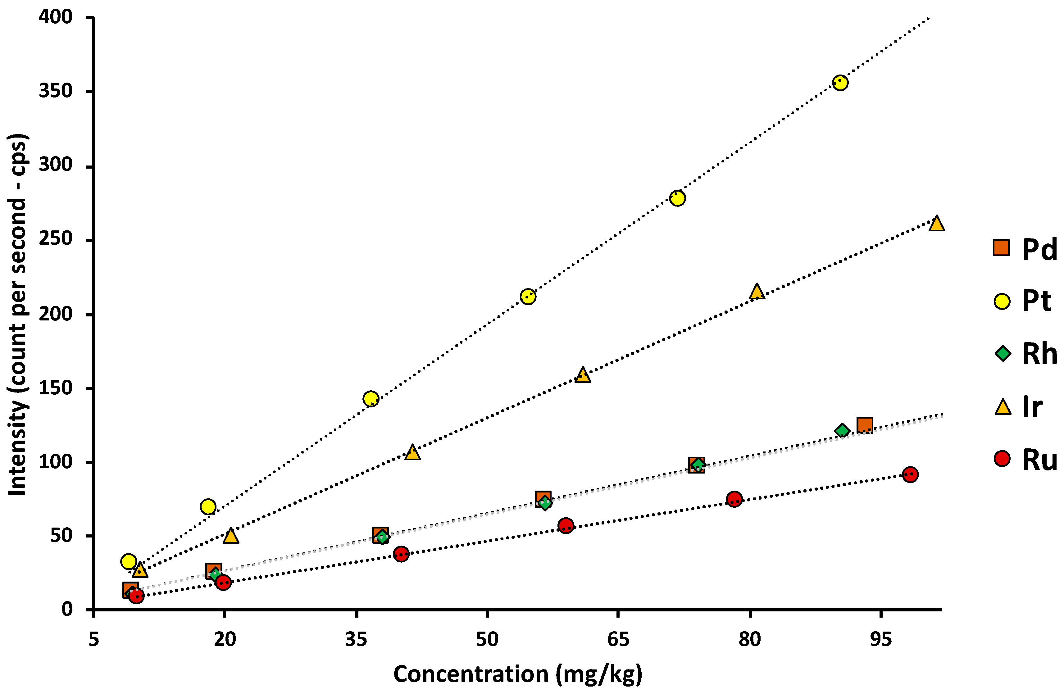
Pd	I = (1,3202 ± 0,0135)[Pd] – (0,6458 ± 0,3817)	0.9999	2,1	7,0
Pt	I = (3,9548 ± 0,0518)[Pt] – (5,1008 ± 2,8498)	0.9998	4,0	13,2
Rh	I = (1,3498 ± 0,0230)[Rh] – (2,2225 ± 1,6218)	0.9995	5,6	18,6
Ru	I = (0,9378 ± 0,0238)[Ru] – (0.6494 ± 1.4237)	0.9994	4,3	14,3
Ir	I = (2,6228 ± 0.0805)[Ir] – (1.1883 ± 4,9621)	0.9991	4,5	15,1

Table 5. t-Test: Paired Two Sample for Means.

	Variable 1	Variable 2
Mean	50,47	47,2816198
Variance	8,57904	11,1645337
Observations	6	6
Pearson Correlation	-0,3341514
Hypothesized Mean Difference	0
df	5
t Stat	1,52334805
P(T<=t) one-tail	0,09408641
t Critical one-tail	2,01504837
P(T<=t) two-tail	0,18817282
t Critical two-tail	2,57058184

Disclaimer/Publisher’s Note: The statements, opinions and data contained in all publications are solely those of the individual author(s) and contributor(s) and not of MDPI and/or the editor(s). MDPI and/or the editor(s) disclaim responsibility for any injury to people or property resulting from any ideas, methods, instructions or products referred to in the content.

© 2023 by the authors. Licensee MDPI, Basel, Switzerland. This article is an open access article distributed under the terms and conditions of the Creative Commons Attribution (CC BY) license (http://creativecommons.org/licenses/by/4.0/).

Copyright: This open access article is published under a Creative Commons CC BY 4.0 license, which permit the free download, distribution, and reuse, provided that the author and preprint are cited in any reuse.

Fast Bimetallic Nanoalloy Quantification Method Using X-ray Fluorescence Spectroscopy for High-Throughput Experiments

Abstract

Keywords:

Subject:

I. Introduction

II. Experimental section

Material

Synthesis

Standard solutions and samples preparation

Characterization and analysis

III. Results and discussion

Synthesis

Method validation

IV. Conclusion

Acknowledgement

References

MDPI Initiatives

Important Links

Subscribe