Convergence and Stability Improvement of Quasi-Newton Methods by Full-Rank Update of the Jacobian Approximates

Preprint

Article

Convergence and Stability Improvement of Quasi-Newton Methods by Full-Rank Update of the Jacobian Approximates

Altmetrics

Downloads

Views

Comments

A peer-reviewed article of this preprint also exists.

Peter Berzi^*

This version is not peer-reviewed

Submitted:

15 November 2023

Posted:

24 November 2023

You are already at the latest version

Alerts

Abstract

A system of simultaneous multi-variable nonlinear equations can be solved by the Newton’s method with local q-quadratic convergence if the Jacobian is analytically available. If this is not the case, then quasi-Newton methods with local q-superlinear convergence give solutions by approximating the Jacobian in some way. Unfortunately, the quasi-Newton condition (secant equation) doesn’t completely specify the Jacobian approximate in multi-dimensional case, so its full-rank update is not possible with classic variants of methods. The suggested new iteration strategy (“T-Secant”) allows full-rank update of the Jacobian approximate in each iteration by determining two independent approximates for the solution. They are used to generate a set of new independent trial approximates, then the Jacobian approximate can fully be updated. It is shown, that the T-Secant approximate is in the vicinity of the classic quasi-Newton approximate, providing that the solution is evenly surrounded by the new trial approximates. The suggested procedure increases the super-linear convergence of the secant method (φS = 1.618...) to super-quadratic (φT = φS + 1 = 2.618...) and the quadratic convergence of the Newton-method (φN = 2) to cubic (φT = φN + 1 = 3) in one dimensional case. The Broyden-type efficiency (mean convergence rate) of the suggested method in multi-dimensional case is an order higher than the efficiency of other classic low-rank update quasi-Newton methods as shown by numerical examples on a Rosenbrock-type test-function with up to 1000 variables. The geometrical representation (hyperbolic approximation) in single variable case helps explaining the basic operations and a vector-space description is also given in multi-variable case.

Keywords:

Subject: Computer Science and Mathematics - Applied Mathematics

1. Introduction

Root-finding methods are essential for solving a great class of numerical problems, such as data fitting problem with

m

sampled data

d = [d_{j}]

(

j = 1, \dots, m

) and

n

adjustable parameters

x = [x_{i}]

(

i = 1, \dots, n

) with

m \geq n

. It leads to the problem of least-squares solving of an overdetermined system of nonlinear equations

f (x) = 0

(1.1)

(

x \in

R^{n}

and

f : R^{n} \to R^{m}

(

m \geq n

)) where the solution

x^{*}

minimizes the difference

{∥f (x)∥}_{2} = ∥ϕ (x) - d∥

₂ between the data

d

and a computational model function

ϕ (x)

. The system of simultaneous multi-variable nonlinear Equations (1.1) can be solved by the Newton’s method when the derivatives of

f (x)

are available analitically and a new iterate

x_{p + 1} = x_{p} - J_{p}^{- 1} f_{p}

(1.2)

that follows

x_{p}

can be determined, where

f_{p} = f (x_{p})

is the function value and

J_{p} = J (x_{p})

is the Jacobian matrix of

f

x_{p}

in the

p^{t h}

iteration step. It is well-known that the local convergence of Newton’s method is q-quadratic if the initial trial approximate

x_{0}

is close enough to the solution

x^{*}

J (x^{*})

is non-singular and

J (x)

satisfies the Lipschitz condition

∥J (x) - J (x^{*})∥ \leq L ∥x - x^{*}∥

(1.3)

for all

x

close enough to

x^{*}

. However, in many cases, the function

ϕ (x)

is not an analytical function, the partial derivatives are not known and Newton’s method cannot be applied. Quasi-Newton methods are defined as the generalization of Equation (1.2) as

x_{p + 1} = x_{p} - B_{p}^{- 1} f_{p}

(1.4)

and

B_{p} ▵ x_{p} = - f_{p}

(1.5)

where

▵ x_{p} = x_{p + 1} - x_{p}

(1.6)

is the iteration step length and

B_{p}

is expected to be the approximate to the Jacobian matrix

J_{p}

without computing derivatives in most cases. The new iterate is then given as

x_{p + 1} = x_{p} + ▵ x_{p}

(1.7)

and

B_{p}

is updated to

B_{p + 1}

according to the specific quasi-Newton method. Martinez [1] has been made a thorough survey on practical quasi-Newton methods. The iterative methods of the form 1.4 that satisfy the equation

B_{p + 1} ▵ x_{p} = f_{p + 1} - f_{p}

(1.8)

for all

k = 0, 1, 2, \dots

are called “quasi-Newton” methods and Equation (1.8) is called the fundamental equation of quasi-Newton methods (“quasi-Newton condition” or “secant equation”). However, the quasi-Newton condition doesn’t uniquely specify the updated Jacobian approximate

B_{p + 1}

and further constraints are needed. Different methods offer their own specific solution. One new quasi-Newton approximate

x_{p + 1}

will never allow full-rank update of

B_{p + 1}

because it is an

n \times n

matrix and only

n

components can be determined from the secant equation, making it an underdetermined system of equations for the elements

[B_{i, j, p + 1}]

(i, j = 1, \dots n)

n > 1

The suggested new strategy is based on Wolfe’s [2] formulation of a generalized secant method. The function

x \to f (x), w h e r e x \in R^{n} a n d f : R^{n} \to R^{n}, n > 1

(1.9)

is locally replaced by linear interpolation through

n + 1

interpolation base points

A_{p}

B_{p, k}

(k = 1, \dots, n)

. The variables

x

and the function values

f

are separated into two equations and an auxiliary variable

q^{A}

is introduced. Then the Jacobian approximate matrix

B_{p}

is split into a variable difference

▵ X_{p}

and a function value difference

▵ F_{p}

matrix and the zero

x_{p + 1}^{A}

of the

p^{th}

interpolation plane is determined from the quasi-Newton condition 1.5 as

[\begin{matrix} ▵ x_{p + 1}^{A} \\ - f_{p}^{A} \end{matrix}] = [\begin{matrix} ▵ X_{p} \\ ▵ F_{p} \end{matrix}] q_{p}^{A}

(1.10)

where

▵ x_{p + 1}^{A} = x_{p + 1}^{A} - x_{p}^{A}

(1.11)

The auxiliary variable

q_{p}^{A}

is determined from the 2^nd row of Equation (1.10) and the new quasi-Newton approximate

x_{p + 1}^{A}

comes from the 1^st row of this equation. Popper [3] made further generalization for functions

x \to f (x), w h e r e x \in R^{n} a n d f : R^{n} \to R^{m}, m \geq n > 1

(1.12)

and suggested to use pseudo-inverse solution for the over determined system of linear equations (where

n

is the number of unknowns and

m

is the number of function values). The auxiliary variable

q_{p}^{A}

is determined from the 2^nd row of Equation (1.10) as

q_{p}^{A} = - ▵ F_{p}^{+} f_{p}^{A}

(1.13)

where

{[.]}^{+}

stands for the pseudo-inverse, and the new quasi-Newton approximate

x_{p + 1}^{A}

comes from the 1^st row of this equation as

x_{p + 1}^{A} = x_{p}^{A} - ▵ X_{p} ▵ {F_{p}}^{+} f_{p}^{A}

(1.14)

The new iteration continues with

n + 1

new base points

A_{p + 1}

B_{p + 1, k}

(k = 1, \dots, n)

. Details are given in Section 3.

Ortega and Rheinboldt [4] stated that a necessary condition of convergence is that the interpolation base points should be linearly independent and they have to be “in general position” through the whole iteration process. Experiences show that the low-rank update procedures often lead to a dead end, because this condition is not satisfied. The purpose of the suggested new iteration strategy is to determine linearly independent base points providing that the Ortega and Rheinboldt condition is satisfied. The basic idea of the procedure is that another new approximate

x_{p + 1}^{B}

is determined from the previous approximate

x_{p + 1}^{A}

and a new system of

n

linearly independent base points is generated. The basic equations of the Wolfe-Popper formulation (Equation (1.10)) were modified as

[\begin{matrix} ▵ x_{p + 1} \\ - f_{p}^{A} \end{matrix}] = [\begin{matrix} T_{p}^{X} & 0 \\ 0 & T_{p}^{F} \end{matrix}] [\begin{matrix} ▵ X_{p} \\ ▵ F_{p} \end{matrix}] q_{p}^{B}

(1.15)

where

▵ x_{p + 1} = x_{p + 1}^{B} - x_{p + 1}^{A}

(1.16)

T_{p}^{X} = d i a g (t_{p, i}^{X}) = diag (\frac{x_{p + 1, i}^{B} - x_{p + 1, i}^{A}}{x_{p + 1, i}^{A} - x_{p, i}^{A}})

(1.17)

and

T_{p}^{F} = diag (t_{p, j}^{F}) = d i a g (\frac{f_{p + 1, j}^{B} - f_{p + 1, j}^{A}}{f_{p + 1, j}^{A} - f_{p, j}^{A}})

(1.18)

The auxiliary variable

q_{p}^{B}

is determined from the 2^nd row of Equation (1.15) as

q_{p}^{B} = - ▵ F_{p}^{+} {(T_{p}^{F})}^{- 1} f_{p}^{A} = - [\sum_{j = 1}^{m} (▵ F_{p, i, j}^{+} \frac{f_{p, j}^{A}}{t_{p, j}^{F}})]

(1.19)

and the new quasi-Newton approximate

x_{p + 1}^{B}

comes from the 1^st row of Equation (1.15) as

x_{p + 1, i}^{B} = x_{p + 1, i}^{A} + \frac{{(▵ x_{p, i}^{A})}^{2}}{▵ x_{p, i} q_{p, i}^{B}} = x_{p + 1, i}^{A} - \frac{{(▵ x_{p, i}^{A})}^{2}}{\sum_{j = 1}^{m} (▵ x_{p, i} ▵ F_{p, i, j}^{+} \frac{f_{p, j}^{A}}{t_{p, j}^{F}})}

(1.20)

(i = 1, \dots, n)

. The details of the proposed new strategy (’T-Secant method’) is given in Section 4. It is different from the traditional secant method in a way, that all interpolation base points

A_{p}

and

B_{p, k}

(k = 1, \dots, n)

are updated in each iteration (full-rank update) providing

n + 1

new base points

A_{p + 1}

and

B_{p + 1, k}

for the next iteration. The key idea of the method is very simple. The function value

f_{p + 1}^{A}

(that can be determined from the new secant approximate

x_{p + 1}^{A}

) measures the ’distance’ of the approximate

x_{p + 1}^{A}

from the root

x^{*}

(if

f_{p + 1}^{A} = 0

, then the distance is zero and

x_{p + 1}^{A} = x^{*}

). The T-secant method uses this information so that the basic equations of the secant method are modified by a scaling transformation

T

, and an additional new estimate

x_{p + 1}^{B}

is determined. Then the new approximates

x_{p + 1}^{A}

and

x_{p + 1}^{B}

are used to construct the

n + 1

new interpolation base points

A_{p + 1}

and

B_{p + 1, k}

The T-secant procedure has been worked out for solving multi-variable problems, it can also be applied for solving single-variable ones, though. The geometrical representation of the latter one gives a good view to explain the mechanism of the procedure as shown in Section 5. It is a surprising result that the T-Secant modification corresponds to a hyperbolic function

z_{p} (x) = \frac{a_{p}}{x - x_{p + 1}^{A}} + f_{p}^{A}

(1.21)

the zero of which gives the second approximate

x_{p + 1}^{B}

in single variable case. A vector space interpretation is also given for the multvariable case in this section.

The general formulations of the proposed method are given in Section 6 and compared with the basic formula of classic quasi-Newton methods. It follows from Equation (1.14) that

S_{p} ▵ x_{p}^{A} = - f_{p}^{A}

(1.22)

where

S_{p} = ▵ F_{p} ▵ X_{p}^{- 1} = [\begin{matrix} \frac{▵ f_{1, 1, p}}{▵ x_{1}} & \dots & \frac{▵ f_{n, 1, p}}{▵ x_{n}} \\ ⋮ & ⋮ & ⋮ \\ \frac{▵ f_{1, m, p}}{▵ x_{1}} & \dots & \frac{▵ f_{n, m, p}}{▵ x_{n}} \end{matrix}] = [\frac{▵ f_{k,, j, p}}{▵ x_{i, p}}]

(1.23)

is the Jacobian approximate of the traditional secant method. It follows from the

1^{st}

and

2^{nd}

rows of Equation (1.15) of the T-Secant method and from the Definition 1.23 of

S_{p}

, that

S_{T, p} ▵ x_{p}^{A} = - f_{p}^{A}

(1.24)

is the modified secant equation, where

S_{T, p} = T_{p}^{F} S_{p} {(T_{p}^{X})}^{- 1} = T_{p}^{F} ▵ F_{p} ▵ X_{p}^{- 1} {(T_{p}^{X})}^{- 1} = [\frac{t_{j, p}^{F}}{t_{i, p}^{X}} \frac{▵ f_{k, j, p}}{▵ x_{i, p}}]

(1.25)

It is well known that the single-variable secant method has asymptotic convergence for sufficiently good initial approximates

x^{A}

and

x^{B}

f^{'} (x)

doesn’t vanish in

x \in [\begin{matrix} x^{A} & x^{B} \end{matrix}]

and

f^{″} (x)

is continuous at least in a neighborhood of the zero

x^{*}

. The super-linear convergence property has been proved in different ways and it is known that the order of convergence is

α = (1 + \sqrt{5}) / 2 = φ

(where

φ = 1.618 . . .

is the golden ratio). The convergence order of the proposed method is determined in Section 7 and it is shown that it has super-quadratic convergence with rate

α^{T S} = φ + 1 = φ^{2} = 2.618 \dots

in single variable case. It is also shown for the multi-variable case in this section, that the second approximate

x_{p + 1}^{B}

will always be in the vicinity of the classic secant approximate

x_{p + 1}^{A}

, providing that the solution

x^{*}

will evenly be surrounded by the

n + 1

new trial approximates, and matrix

S_{p + 1}

will be well-conditioned.

A step-by-step algorithm is given in Section 8 and the results of numerical tests with a Rosenbrock-type test function demonstrates the stability of the proposed strategy in Section 9 for up to 1000 unknown variables. The Broyden-type efficiency (mean convergence rate) of the proposed method is studied in multi-variable case in Section 10 and it is compared with other classic rank-one update and line-search methods on the basis of available test data. It is shown in Section 11 how the new procedure can be used to improve the convergence of other classic multi-variable root finding methods (Newton-Raphson and Broyden methods). Concluding remarks are summarized in Section 12. Among others, the method has been used for the identification of vibrating mechanical systems (foundation pile driving [5], percussive drilling [6]) and found to be very stable and efficient even in case of large number of unknowns.

The proposed method needs

n + 1

function value evaluations in each iteration and it is not using the derivative information of the function, like the Newton-Raphson method is doing. On the other hand, it needs

n

more function evaluations than the traditional secant method needs in each iteration. However, it is an apparent disadvantage, as the convergence rate considerably increases (

α^{TS} ≅ 2.618 . . .

), furthermore the stability and the efficiency of the procedure has been highly improved.

2. Notations

Vectors and matrices are denoted by bold-face letters. Subscripts refer to components of vectors and matrices, superscripts

A

and

B

refer to interpolation base points. Vectors and matrices may also be given by their general elements.

▵

refers to a difference of two elements.

x

and

X

denotes unknown quantities,

f

and

F

denotes function values and matrices.

q

q

t

, and

T

denotes multiplier scalars, vectors and matrices.

e

ε

and

E

denotes approximate error,

p

is iteration counter,

α

is convergence rate,

ε^{*}

is termination criterion.

n

is the number of unknowns,

m

is the number of function values,

i

j

k

and l are running indexes of matrix columns and rows. Superscripts

S

and

TS

refer to the traditional Secant-method and to the proposed T-Secant method receptively.

3. Secant method

The history of the secant method in single variable case is several thousands years old, its origin was found in ancient time. The idea of finding the scalar root

x^{*}

of a scalar nonlinear function

x \to f (x) (w h e r e x \in R^{1} a n d f : R^{1} \to R^{1})

(3.1)

by successive local replacement of the function by linear interpolation (secant line) gives a simple and efficient numerical procedure. It has an advantage that it doesn’t need the calculation of function derivatives, it only uses function values and the order of asymptotic convergence is super-linear with convergence rate

α^{S} ≅ 1.618 . . .

The function

f (x)

is locally replaced by linear interpolation (secant line) through interpolation base points

A

and

B

and the zero

x^{A}

of the secant line is determined as an approximate to the zero

x^{*}

of the function. The next iteration continues with new base points, selected from available old ones. Wolfe [2] extended the scalar procedure to multidimensional

x \to f (x), w h e r e x \in R^{n} a n d f : R^{n} \to R^{n}, n > 1

(3.2)

and Popper [3] made further generalization

x \to f (x), w h e r e x \in R^{n} a n d f : R^{n} \to R^{m}, m \geq n > 1

(3.3)

and suggested to use pseudo-inverse solution for the over determined system of linear equations (where

n

is the number of unknowns and

m

is the number of function values).

The zero

x^{*}

of the nonlinear function

x \to f (x)

has to be found, where

x \in

R^{n}

and

f : R^{n} \to R^{m}

. Let

x^{A}

be the initial trial for the zero

x^{*}

, and let the function

f (x)

be linearly interpolated through

n + 1

interpolation base points

A (\begin{matrix} x^{A} & f^{A} \end{matrix})

and

B_{k} (\begin{matrix} x_{k}^{B} & f_{k}^{B} \end{matrix})

(k = 1, \dots, n)

and be approximated / replaced by the interpolation “plane”

y (x)

near

x^{*}

. One of the key ideas of the suggested numerical procedure is that interpolation base points

B_{k} (\begin{matrix} x_{k}^{B} & f_{k}^{B} \end{matrix})

are constructed by individually increment the coordinates

x_{i}^{A}

of the initial trial

x^{A}

by an “initial trial increment” value

▵ x_{i}

(i = 1, \dots, n)

x_{k, i}^{B} = x_{i}^{A} + ▵ x_{i}

(3.4)

or in vector form as

x_{k}^{B} = x^{A} + ▵ x_{k} d^{k}

(3.5)

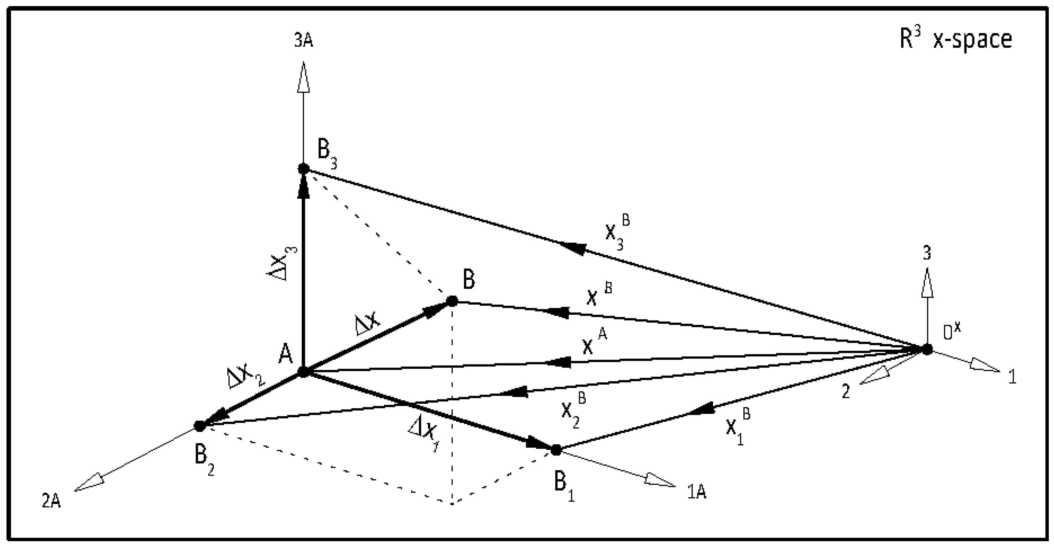
where

d^{k}

is the

k^{t h}

Cartesian unit vector as shown on Figure 1.

It follows from this special construction of the initial trials

x_{k}^{B}

, that

x_{k, i}^{B} - x_{i}^{A} = 0

for

i \neq k

and

x_{k, i}^{B} - x_{i}^{A} = ▵ x_{i}

for

i = k

providing that

▵ x = [x_{i, i}^{B} - x_{i}^{A}] = [▵ x_{i}]

(3.6)

is the “initial trial increment vector”. Let

▵ f_{k} = [▵ f_{k, j}] = [f_{k, j}^{B} - f_{j}^{A}]

(3.7)

(j = 1, \dots, m)

. Any point on the

n

dimensional interpolation plane

y (x)

can be expressed as

[\begin{matrix} x \\ y (x) \end{matrix}] = [\begin{matrix} x^{A} \\ f^{A} \end{matrix}] + [\begin{matrix} ▵ X \\ ▵ F \end{matrix}] q^{A}

(3.8)

where

▵ X = [x_{k}^{B} - x^{A}] = [\begin{matrix} x_{1, 1}^{B} - x_{1}^{A} & \dots & x_{n, 1}^{B} - x_{1}^{A} \\ ⋮ & ⋱ & ⋮ \\ x_{1, n}^{B} - x_{n}^{A} & \dots & x_{n, n}^{B} - x_{n}^{A} \end{matrix}]

(3.9)

▵ F = [f_{k}^{B} - f^{A}] = [\begin{matrix} f_{1, 1}^{B} - f_{1}^{A} & \dots & f_{n, 1}^{B} - f_{1}^{A} \\ ⋮ & ⋮ & ⋮ \\ f_{1, m}^{B} - f_{m}^{A} & \dots & f_{n, m}^{B} - f_{m}^{A} \end{matrix}]

(3.10)

(k = 1, \dots, n)

q^{A}

is a vector with

n

scalar multipliers

q_{i}^{A}, (i = 1, \dots, n)

and as a consequence of Equation (3.5)

▵ X = [▵ x_{k}] = [\begin{matrix} ▵ x_{1} & \dots & 0 \\ ⋮ & ⋱ & ⋮ \\ 0 & \dots & ▵ x_{n} \end{matrix}] = d i a g (▵ x_{i})

(3.11)

is a diagonal matrix that has great computational advantage. It also follows from Definition 3.7 that

▵ F = [▵ f_{k}] = [\begin{matrix} ▵ f_{1, 1} & \dots & ▵ f_{n, 1} \\ ⋮ & ⋮ & ⋮ \\ ▵ f_{1, m} & \dots & ▵ f_{n, m} \end{matrix}]

(3.12)

Let

x_{p + 1}^{A}

be the zero of the n-dimensional interpolation plane

y_{p} (x)

in the

p^{th}

iteration with interpolation base points

A_{p} (\begin{matrix} x_{p}^{A} & f_{p}^{A} \end{matrix})

and

B_{k, p} (\begin{matrix} x_{k, p}^{B} & f_{k, p}^{B} \end{matrix})

. Then it follows from the zero condition

y_{p} (x_{p + 1}^{A}) = 0

(3.13)

and from the

2^{nd}

row of Equation (3.8) that

▵ F_{p} q_{p}^{A} = - f_{p}^{A}

(3.14)

and the vector

q_{p}^{A}

of multipliers

q_{p, i}^{A}

can be expressed as

q_{p}^{A} = - ▵ F_{p}^{+} f_{p}^{A}

(3.15)

where

{[.]}^{+}

stands for the pseudo-inverse. Let

[\begin{matrix} ▵ x_{p}^{A} \\ ▵ f_{p}^{A} \end{matrix}] = [\begin{matrix} x_{p + 1}^{A} - x_{p}^{A} \\ f_{p + 1}^{A} - f_{p}^{A} \end{matrix}]

(3.16)

be the iteration step-size of the secant method, then it follows from the

1^{st}

row of Equation (3.8) and from Equation (3.15), that

▵ x_{p}^{A} = ▵ X_{p} q_{p}^{A} = - ▵ X_{p} ▵ F_{p}^{+} f_{p}^{A}

(3.17)

and from Definition 3.16 it follows that

[\begin{matrix} x_{p + 1}^{A} \\ f_{p + 1}^{A} \end{matrix}] = [\begin{matrix} x_{p}^{A} + ▵ x_{p}^{A} \\ f_{p}^{A} + ▵ f_{p}^{A} \end{matrix}]

(3.18)

and the new secant approximate

x_{p + 1}^{A}

can be expressed from Equation (3.17) as

x_{p + 1}^{A} = x_{p}^{A} + ▵ x_{p}^{A}

(3.19)

A base point

A_{p + 1} (x_{p + 1}^{A}, f_{p + 1}^{A})

and base vector

v_{p + 1}^{A} = (x_{p + 1}^{A}, f_{p + 1}^{A})

can than be determined for the next iteration. In single variable case

(m = n = k = 1)

with interpolation base points

A_{p} (x_{p}^{A}, f_{p}^{A})

and

B_{p} (x_{p}^{B}, f_{p}^{B})

, Equation (3.15) will have the form

q_{p}^{A} = - \frac{f_{p}^{A}}{f_{p}^{B} - f_{p}^{A}} = - \frac{f_{p}^{A}}{▵ f_{p}}

(3.20)

and the new secant approximate

x_{p + 1}^{A} = x_{p}^{A} + ▵ x_{p} q_{p}^{A} = x_{p}^{A} - \frac{▵ x_{p}}{▵ f_{p}} f_{p}^{A} = \frac{x_{p}^{A} f_{p}^{B} - x_{p}^{B} f_{p}^{A}}{f_{p}^{B} - f_{p}^{A}}

(3.21)

can be determined according to Equation (3.19). The procedure then continues with interpolation base points

A_{p + 1} (x_{p + 1}^{A}, f_{p + 1}^{A})

and

B_{p + 1} (x_{p + 1}^{B}, f_{p + 1}^{B})

4. T-Secant method

4.1. Single-variable case

The T-secant method is different from the traditional secant method in a way, that all interpolation base points

A_{p}

and

B_{p, k}

(k = 1, \dots, n)

are updated in each iteration providing

n + 1

new base points

A_{p + 1}

and

B_{p + 1, k}

for the next iteration. The key idea of the method is very simple. The function value

f_{p + 1}^{A}

(that can be determined from the new secant approximate

x_{p + 1}^{A}

) measures the ’distance’ of the approximate

x_{p + 1}^{A}

from the root

x^{*}

(if

f_{p + 1}^{A} = 0

, then the distance is zero and

x_{p + 1}^{A} = x^{*}

). The T-secant method uses this information to determine another approximate

x_{p + 1}^{B}

. In single variable case

(m = n = k = 1)

with interpolation base points

A_{p}

and

B_{p}

, the basic equation

▵ f_{p} q_{p}^{A} = - f_{p}^{A}

(4.1)

of the secant method (Equation (3.14) in multi-variable case) is modified by a factor

t_{p}^{f} = \frac{f_{p + 1}^{A}}{f_{p}^{A}}

(4.2)

that expresses the ’improvement rate’ of the new approximate

x_{p + 1}^{A}

to the original approximate

x_{p}^{A}

, providing the T-secant modified basic equation

t_{p}^{f} ▵ f_{p} q_{p}^{B} = - f_{p}^{A}

(4.3)

Then the T-secant multiplier

q_{p}^{B} = \frac{q_{p}^{A}}{t_{p}^{f}} = - \frac{{(f_{p}^{A})}^{2}}{f_{p + 1}^{A} ▵ f_{p}}

(4.4)

can be determined. The other basic equation

▵ x_{p}^{A} = ▵ x_{p} q_{p}^{A}

(4.5)

of the secant method (Equation (3.17) in multi-variable case) with iteration step size

▵ x_{p}^{A} = x_{p + 1}^{A} - x_{p}^{A}

(4.6)

is also modified in a similar way like in case of Equation (4.1) and Equation (4.3) by a factor

t_{p}^{x} = \frac{x_{p + 1}^{B} - x_{p + 1}^{A}}{x_{p + 1}^{A} - x_{p}^{A}} = \frac{▵ x_{p + 1}}{▵ x_{p}^{A}}

(4.7)

that expresses the ’improvement rate’ of the new ’T-secant approximate change’

▵ x_{p + 1}

to the previous ’secant iteration step size’

▵ x_{p}^{A}

, providing a new basic equation

▵ x_{p}^{A} = t_{p}^{x} ▵ x_{p} q_{p}^{B}

(4.8)

from which

▵ x_{p}^{A} = \frac{▵ x_{p + 1}}{▵ x_{p}^{A}} ▵ x_{p} q_{p}^{B}

(4.9)

and

x_{p + 1}^{A} - x_{p}^{A} = - \frac{x_{p + 1}^{B} - x_{p + 1}^{A}}{x_{p + 1}^{A} - x_{p}^{A}} (x_{p}^{B} - x_{p}^{A}) \frac{{(f_{p}^{A})}^{2}}{f_{p + 1}^{A} (f_{p}^{B} - f_{p}^{A})}

(4.10)

By re-ordering Equation (4.10), the T-secant approximate

x_{p + 1}^{B} = x_{p + 1}^{A} + \frac{{(▵ x_{p}^{A})}^{2}}{▵ x_{p} q_{p}^{B}} = x_{p + 1}^{A} - \frac{{(x_{p + 1}^{A} - x_{p}^{A})}^{2} (f_{p}^{B} - f_{p}^{A}) f_{p + 1}^{A}}{(x_{p}^{B} - x_{p}^{A}) {(f_{p}^{A})}^{2}}

(4.11)

can be determined and it is used to update the original interpolation base point

B_{p}

B_{p + 1}

. The new iteration will then continue with new base points

A_{p + 1}

and

B_{p + 1}

. Note, that it follows from Equations (4.4), (4.5) and (4.11) that

▵ x_{p + 1} = x_{p + 1}^{B} - x_{p + 1}^{A} = \frac{{(▵ x_{p}^{A})}^{2}}{▵ x_{p} q_{p}^{B}} = t_{p}^{f} \frac{{(▵ x_{p}^{A})}^{2}}{▵ x_{p} q_{p}^{A}} = t_{p}^{f} ▵ x_{p}^{A}

(4.12)

4.2. Multi-variable case

In multi-variable case

(m \geq n > 1)

with

(n + 1)

interpolation base points

A_{p} (\begin{matrix} x_{p}^{A} & f_{p}^{A} \end{matrix})

and

B_{p, k} (\begin{matrix} x_{p, k}^{B} & f_{p, k}^{B} \end{matrix})

(k = 1, \dots, n)

, the basic equations of the secant method (Equation (3.14) and 3.17) are modified as

T_{p}^{F} ▵ F_{p} q_{p}^{B} = - f_{p}^{A}

(4.13)

and

▵ x_{p}^{A} = T_{p}^{X} ▵ X_{p} q_{p}^{B}

(4.14)

Then a vector based equation can be formulated like in case of the traditional secant method (see Equation (3.8)) in a form

[\begin{matrix} x - ▵ x \\ z (x) \end{matrix}] = [\begin{matrix} x^{A} \\ f^{A} \end{matrix}] + [\begin{matrix} T^{X} & 0 \\ 0 & T^{F} \end{matrix}] [\begin{matrix} ▵ X \\ ▵ F \end{matrix}] q^{B}

(4.15)

where

▵ X

and

▵ F

are defined in 3.9 and 3.10,

z (x)

is a function with zero at

x_{p + 1}^{B}

and the diagonal transformation matrix in the

p^{th}

iteration is

T_{p} = [\begin{matrix} T_{p}^{X} & 0 \\ 0 & T_{p}^{F} \end{matrix}]

(4.16)

with

T_{p}^{X}

and

T_{p}^{F}

sub-diagonals, where

T_{p}^{X} = d i a g (t_{p, i}^{X}) = diag (\frac{x_{p + 1, i}^{B} - x_{p + 1, i}^{A}}{x_{p + 1, i}^{A} - x_{p, i}^{A}}) = diag (\frac{▵ x_{p + 1, i}}{▵ x_{p, i}^{A}})

(4.17)

T_{p}^{F} = diag (t_{p, j}^{F}) = d i a g (\frac{f_{p + 1, j}^{B} - f_{p + 1, j}^{A}}{f_{p + 1, j}^{A} - f_{p, j}^{A}})

(4.18)

and

T_{p}^{F}

is approximated with the assumption

f (x) ≃ y_{p} (x_{p + 1}^{A}) ≃ z_{p} (x_{p + 1}^{B})

and according to the conditions

y_{p} (x_{p + 1}^{A}) = 0

and

z_{p} (x_{p + 1}^{B}) = 0

T_{p}^{F} ≃ diag (\frac{z_{p, j} (x_{p + 1}^{B}) - f_{p + 1, j}^{A}}{y_{p, j} (x_{p + 1}^{A}) - f_{p, j}^{A}}) = d i a g (\frac{f_{p + 1, j}^{A}}{f_{p, j}^{A}})

(4.19)

(i = 1, \dots, n)

(j = 1, \dots, m)

, where

f_{p, j}^{A} \neq 0

. The vector of T-secant multipliers

q_{p}^{B} = - ▵ F_{p}^{+} {(T_{p}^{F})}^{- 1} f_{p}^{A} = - [\sum_{j = 1}^{m} (▵ F_{p, i, j}^{+} \frac{f_{p, j}^{A}}{t_{p, j}^{F}})]

(4.20)

can be determined from Equation (4.13) , where

{[.]}^{+}

stands for the pseudo-inverse (

▵ F_{p}^{+}

has already been calculated when

q_{p}^{A}

was determined from Equation (3.15)). The

i^{th}

element of the new approximate

x_{p + 1}^{B}

can be expressed from the

i^{th}

row of Equation (4.14) as

▵ x_{p, i}^{A} = \frac{▵ x_{p + 1, i}}{▵ x_{p, i}^{A}} ▵ x_{p, i} q_{p, i}^{B} = \frac{x_{p + 1, i}^{B} - x_{p + 1, i}^{A}}{▵ x_{p, i}^{A}} ▵ x_{p, i} q_{p, i}^{B}

(4.21)

and the T-Secant approximate

x_{p + 1}^{B}

can be calculated as

x_{p + 1, i}^{B} = x_{p + 1, i}^{A} + \frac{{(▵ x_{p, i}^{A})}^{2}}{▵ x_{p, i} q_{p, i}^{B}} = x_{p + 1, i}^{A} - \frac{{(▵ x_{p, i}^{A})}^{2}}{\sum_{j = 1}^{m} (▵ x_{p, i} ▵ F_{p, i, j}^{+} \frac{f_{p, j}^{A}}{t_{p, j}^{F}})}

(4.22)

where

▵ x_{p, i} \neq 0

and

q_{p, i}^{B} \neq 0

(i = 1, \dots, n)

. Then the next iteration continues with the new trial increment vector

▵ x_{p + 1} = x_{p + 1}^{B} - x_{p + 1}^{A}

(4.23)

and with

n + 1

new interpolation base points

A_{p + 1} (\begin{matrix} x_{p + 1}^{A} & f_{p + 1}^{A} \end{matrix})

B_{k, p + 1} (\begin{matrix} x_{k, p + 1}^{B} & f_{k, p + 1}^{B} \end{matrix})

(k = 1, \dots, n)

. Figure 1 shows the formulation of a set of new base vectors

x_{k, p + 1}^{B}

from

x_{p + 1}^{A}

and

x_{p + 1}^{B}

n = 3

case.

Table 1. Summary of the basic equations (single- and multi-variable cases).

	Single-variable $(m = n = 1)$	Multi-variable $(m \geq n > 1)$	Equations
1	$x_{p}^{A}$	$x_{p}^{A}$
2	$x_{p}^{B}$	$x_{p, k}^{B} = x_{p}^{A} + ▵ x_{p, k} d^{k}$	3.5
3	$▵ x_{p} = x_{p}^{B} - x_{p}^{A}$	$▵ X_{p} = [x_{p, k}^{B} - x_{p}^{A}] = d i a g (▵ x_{p, i})$	3.9, 3.11
4	$▵ f_{p} = f_{p}^{B} - f_{p}^{A}$	$▵ F_{p} = [\begin{matrix} ▵ f_{p, 1, 1} & \dots & ▵ f_{p, n, 1} \\ ⋮ & ⋱ & ⋮ \\ ▵ f_{p, 1, m} & \dots & ▵ f_{p, n, m} \end{matrix}]$	3.7, 3.10, 3.12
5	$▵ f_{p} q_{p}^{A} = - f_{p}^{A}$	$▵ F_{p} q_{p}^{A} = - f_{p}^{A}$	4.1, 3.14
6	$q_{p}^{A} = - \frac{f_{p}^{A}}{▵ f_{p}}$	$q_{p}^{A} = - ▵ F_{p}^{+} f_{p}^{A}$	3.20, 3.15
7	$x_{p + 1}^{A} = x_{p}^{A} + ▵ x_{p} q_{p}^{A}$	$x_{p + 1}^{A} = x_{p}^{A} + ▵ X_{p} q_{p}^{A}$	3.21, 3.19
8	$▵ x_{p}^{A} = x_{p + 1}^{A} - x_{p}^{A}$	$▵ x_{p}^{A} = x_{p + 1}^{A} - x_{p}^{A}$	4.6
9	$t_{p}^{f} = \frac{f_{p + 1}^{A}}{f_{p}^{A}}$	$T_{p}^{F} = d i a g (\frac{f_{p + 1, j}^{A}}{f_{p, j}^{A}})$	4.2, 4.19
10	$t_{p}^{f} ▵ f_{p} q_{p}^{B} = - f_{p}^{A}$	$T_{p}^{F} ▵ F_{p} q_{p}^{B} = - f_{p}^{A}$	4.3, 4.13
11	$q_{p}^{B} = \frac{q_{p}^{A}}{t_{p}^{f}} = - \frac{{(f_{p}^{A})}^{2}}{f_{p + 1}^{A} ▵ f_{p}}$	$q_{p}^{B} = - ▵ F_{p}^{+} {(T_{p}^{F})}^{- 1} f_{p}^{A}$	4.4, 4.20
12	$t_{p}^{x} = \frac{x_{p + 1}^{B} - x_{p + 1}^{A}}{x_{p + 1}^{A} - x_{p}^{A}} = \frac{▵ x_{p + 1}}{▵ x_{p}^{A}}$	$T_{p}^{X} = diag (\frac{▵ x_{p + 1, i}}{▵ x_{p, i}^{A}})$	4.7, 4.17
13	$▵ x_{p}^{A} = t_{p}^{x} ▵ x_{p} q_{p}^{B}$	$▵ x_{p}^{A} = T_{p}^{X} ▵ X_{p} q_{p}^{B}$	4.8, 4.14
14	$x_{p + 1}^{B} = x_{p + 1}^{A} + \frac{{(▵ x_{p}^{A})}^{2}}{▵ x_{p} q_{p}^{B}}$	$x_{p + 1, i}^{B} = x_{p + 1, i}^{A} + \frac{{(▵ x_{p, i}^{A})}^{2}}{▵ x_{p, i} q_{p, i}^{B}}$	4.11, 4.22

5. Geometry

5.1. Single-variable case

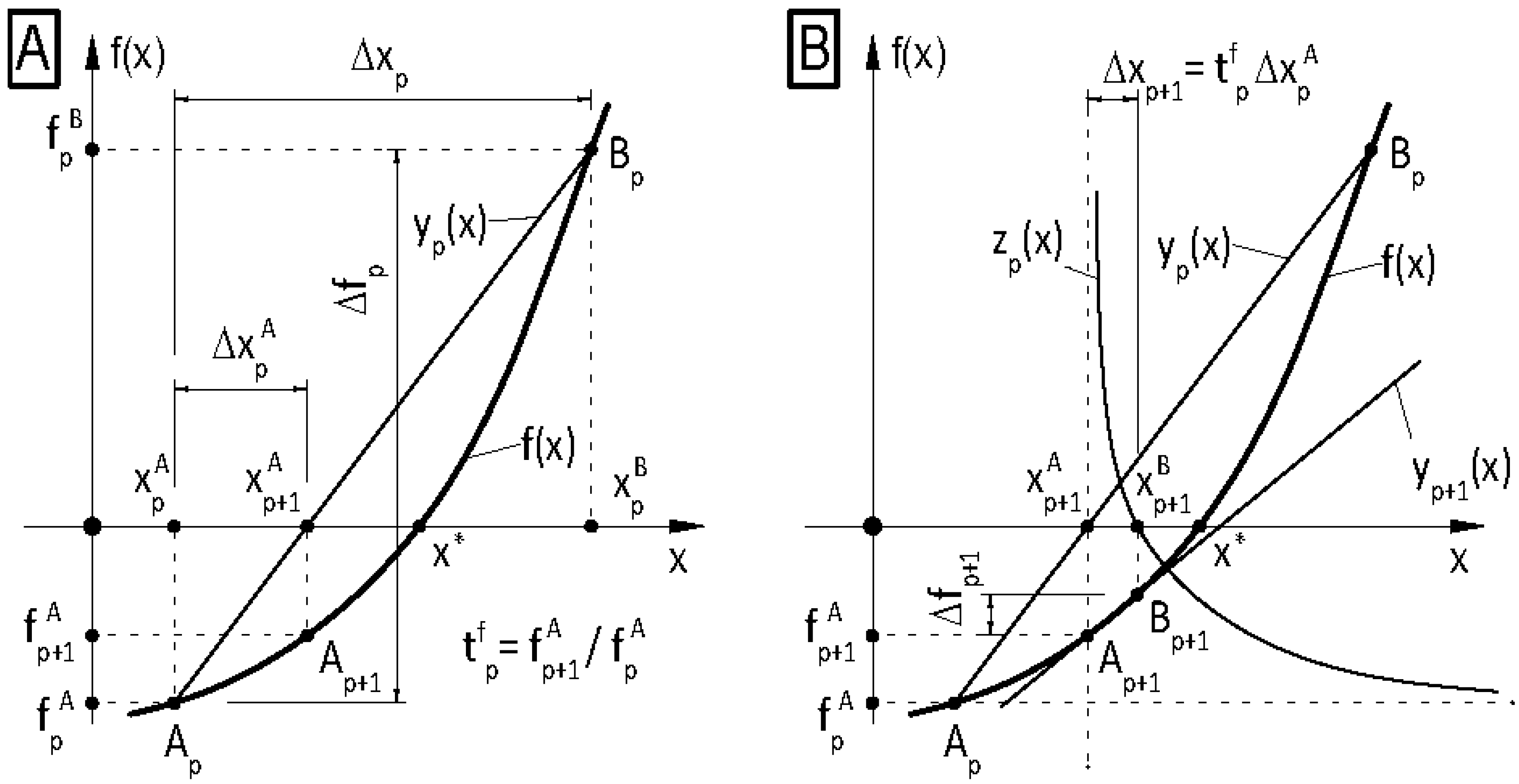
Find the scalar root

x^{*}

of a nonlinear function

x \to f (x)

, where

x \in R^{1}

and

f : R^{1} \to R^{1}

. Let the function

f (x)

be linearly interpolated through initial base points

A_{p} (x_{p}^{A}, f_{p}^{A})

and

B_{p} (x_{p}^{B}, f_{p}^{B})

providing a “secant” line

y_{p} (x)

as shown on Figure 2, where

f_{p}^{A} = f (x_{p}^{A})

and

f_{p}^{B} = f (x_{p}^{B})

are the corresponding function values. An arbitrary point of the secant

y_{p} (x)

can be expressed as

[\begin{matrix} x \\ y_{p} (x) \end{matrix}] = [\begin{matrix} x_{p}^{A} \\ f_{p}^{A} \end{matrix}] + [\begin{matrix} ▵ x_{p} \\ ▵ f_{p} \end{matrix}] q_{p}^{A}

(5.1)

where

q_{p}^{A}

is a scalar multiplier. Let a new approximate

x_{p + 1}^{A}

be the root of the secant

y_{p} (x)

and let

▵ x_{p}^{A} = x_{p + 1}^{A} - x_{p}^{A}

(5.2)

be the iteration step size. It follows from condition

y_{p} (x_{p + 1}^{A}) = 0

(5.3)

and from the

2^{nd}

row of Equation (5.1) that

▵ f_{p} q_{p}^{A} = - f_{p}^{A}

(5.4)

and the scalar multiplier can be determined as

q_{p}^{A} = - \frac{f_{p}^{A}}{▵ f_{p}}

(5.5)

From the

1^{st}

row of Equation (5.1), the iteration step size is given as

▵ x_{p}^{A} = ▵ x_{p} q_{p}^{A}

(5.6)

and the new approximate can be expressed as

x_{p + 1}^{A} = x_{p}^{A} + ▵ x_{p}^{A}

(5.7)

A new base point

A_{p + 1} (x_{p + 1}^{A}, f_{p + 1}^{A})

(see Figure 2) can than be determined for the next iteration. Two out of the three available base points

(\begin{matrix} A_{p} & B_{p} & A_{p + 1} \end{matrix})

are used for the next iteration by omitting either

A_{p}

B_{p}

in case of the traditional secant method. Decision is not obvious and it may cause that the iteration will be unstable and / or will not converge to the solution. Instead, an additional new approximate

x_{p + 1}^{B}

is determined by the T-secant procedure as a root of the function

z_{p} (x)

near the first secant approximate

x_{p + 1}^{A}

, and iteration continues with new base points

A_{p + 1} (x_{p + 1}^{A}, f_{p + 1}^{A})

and

B_{p + 1} (x_{p + 1}^{B}, f_{p + 1}^{B})

. An arbitrary point of the function

z_{p} (x)

can be expressed as

[\begin{matrix} x - ▵ x \\ z_{p} (x) \end{matrix}] = [\begin{matrix} x_{p}^{A} \\ f_{p}^{A} \end{matrix}] + [\begin{matrix} t^{x} & 0 \\ 0 & t^{f} \end{matrix}] [\begin{matrix} ▵ x_{p} \\ ▵ f_{p} \end{matrix}] q_{p}^{B}

(5.8)

where the transformation scalars for

▵ x_{p}

and

▵ f_{p}

x = x_{p}^{B}

are

t_{p}^{x} = \frac{▵ x_{p + 1}}{▵ x_{p}^{A}} = \frac{x_{p + 1}^{B} - x_{p + 1}^{A}}{x_{p + 1}^{A} - x_{p}^{A}} a n d t_{p}^{f} = \frac{f_{p + 1}^{A}}{f_{p}^{A}}

(5.9)

Then it follows from condition

z_{p} (x_{p + 1}^{B}) = 0

(5.10)

and from the

2^{nd}

row of Equation (5.8) that

t_{p}^{f} ▵ f_{p} q_{p}^{B} = - f_{p}^{A}

(5.11)

and

q_{p}^{B} = - \frac{f_{p}^{A}}{t_{p}^{f} ▵ f_{p}} = - \frac{{(f_{p}^{A})}^{2}}{f_{p + 1}^{A} (f_{p}^{B} - f_{p}^{A})}

(5.12)

The new approximate

x_{p + 1}^{B}

can then be expressed from the

1^{st}

row of Equation 5.8, as

x_{p + 1}^{B} = x_{p + 1}^{A} + \frac{{(▵ x_{p}^{A})}^{2}}{▵ x_{p} q_{p}^{B}}

(5.13)

The new base point

B_{p + 1} (x_{p + 1}^{B}, f_{p + 1}^{B})

(see Figure 2) then can be determined. Interpolation base points

A_{p + 1}

and

B_{p + 1}

are used for the next iteration. The scalar multiplier

q_{p}^{B}

can be expressed from Equation (5.13) as

q_{p}^{B} = \frac{{(x_{p + 1}^{A} - x_{p}^{A})}^{2}}{(x_{p}^{B} - x_{p}^{A}) (x_{p + 1}^{B} - x_{p + 1}^{A})}

(5.14)

By substituting it into the

2^{nd}

row of Equation 5.8 and changing

x_{p + 1}^{B}

x

, it turns to a hyperbolic function

z_{p} (x) = \frac{a_{p}}{x - x_{p + 1}^{A}} + f_{p}^{A}

(5.15)

with vertical and horizontal asymptotes

x_{p + 1}^{A}

and

f_{p}^{A}

, where

a_{p} = {(x_{p + 1}^{A} - x_{p}^{A})}^{2} \frac{f_{p}^{B} - f_{p}^{A}}{x_{p}^{B} - x_{p}^{A}} \frac{f_{p + 1}^{A}}{f_{p}^{A}}

(5.16)

and the root

x_{p + 1}^{B}

of the function

z_{p} (x)

will be in the vicinity of

x_{p + 1}^{A}

in “appropriate distance” that is regulated by the function value

f_{p + 1}^{A}

(see Figure 2). This virtue of the T-secant procedure ensures an automatic mechanism for having base vectors in general positions through the whole iteration process providing stable and efficient numerical performance.

5.2. Multi-variable case

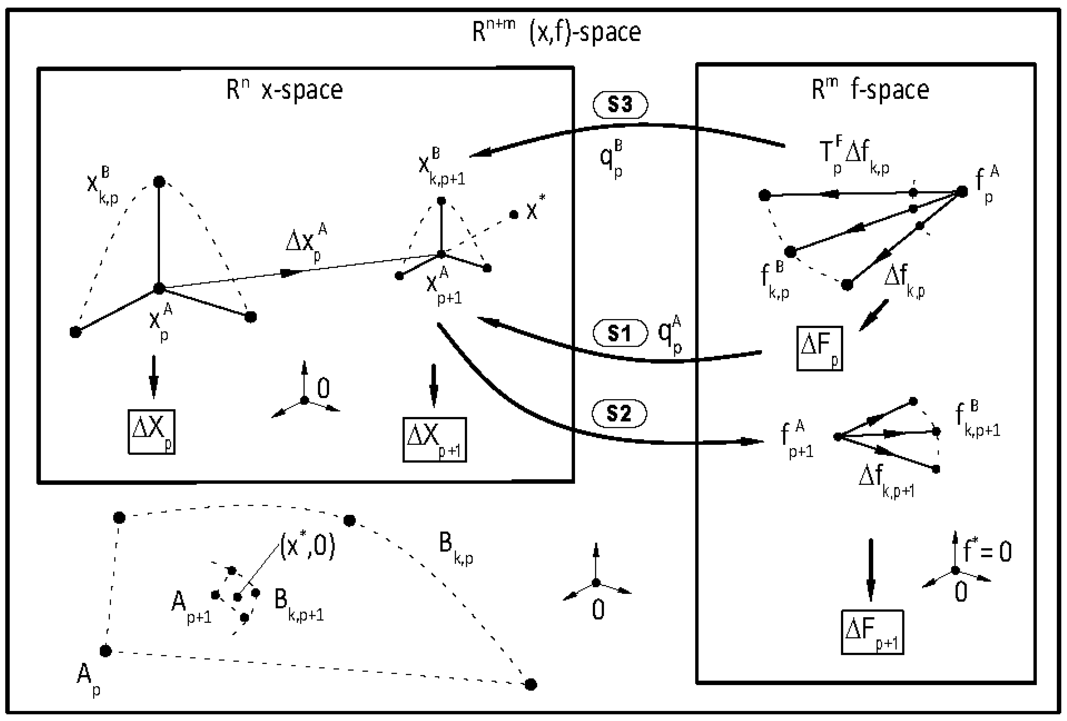
Find the root

x^{*}

of a nonlinear function

x \to f (x)

, where

x \in R^{n}

and

f : R^{n} \to R^{m}

. Let the function

f (x)

be linearly interpolated through

n + 1

base points

A_{p} (x_{p}^{A}, f_{p}^{A})

and

B_{k, p} (x_{k, p}^{B}, f_{k, p}^{B})

in the

R^{n + m}

space (

f (x) -

space) in the

p^{th}

iteration as shown on Figure 3, where

k = 1, \dots, n

. Given a set of approximates

x_{p}^{A}

and

x_{k, p}^{B} = x_{p}^{A} + ▵ x_{k, p} d^{k}

(5.17)

in the

R^{n}

space (

x -

space) with

k = 1, \dots, n

, where

d^{k}

is the

k^{t h}

Cartesian unit vector. Let the expression

▵ F_{p} q_{p}^{A} = [\begin{matrix} ▵ f_{1, 1, p} & \dots & ▵ f_{n, 1, p} \\ ⋮ & ⋮ & ⋮ \\ ▵ f_{1, m, p} & \dots & ▵ f_{n, m, p} \end{matrix}] q_{p}^{A}

(5.18)

represent the linear combination

q_{p}^{A} = {[q_{p, k}^{A}]}^{T}

n

column vectors

[▵ f_{k, j, p}] = [▵ f_{k, p}] = [f_{k, p}^{B} - f_{k, p}^{A}]

in the

R^{m}

space (

f -

space) with

k = 1, \dots, n

column index and with

j = 1, \dots, m

row index and the expression

▵ X_{p} q_{p}^{A} = [\begin{matrix} ▵ x_{1, 1, p} & \dots & ▵ x_{n, 1, p} \\ ⋮ & ⋮ & ⋮ \\ ▵ x_{1, n, p} & \dots & ▵ x_{n, n, p} \end{matrix}] q_{p}^{A}

(5.19)

represent the same linear combination of

n

column vectors

[▵ x_{k, j, p}] = [▵ x_{p, k}] = [x_{p, k}^{B} - x_{p, k}^{A}]

(5.20)

with

k = 1, \dots, n

column index and with

j = 1, \dots, n

row index. The linear combination

q_{p}^{A}

is determined from Equation (3.15) in step

S 1

(see Figure 3) providing a new approximate

x_{p + 1}^{A} = [x_{p + 1, k}^{A}] = x_{p}^{A} + ▵ x_{p}^{A}

(5.21)

for the solution

x^{*}

as shown on Figure 3 and the corresponding

f_{p + 1}^{A}

vector is also determined in step

S 2

(see Figure 3). The column vectors

▵ f_{k, p}

▵ F_{p}

are then modified by a non-uniform scaling transformation

T_{p}^{F} = d i a g (\frac{f_{p + 1, j}^{A}}{f_{p, j}^{A}})

(5.22)

and a new linear combination

q_{p}^{B} = {[q_{p, k}^{B}]}^{T}

is determined from Equation (4.20) in step

S 3

(see Figure 3) providing a new approximate

x_{p + 1}^{B}

for the solution

x^{*}

with elements

x_{p + 1, k}^{B} = x_{p + 1, k}^{A} + \frac{{(▵ x_{p, k}^{A})}^{2}}{▵ x_{p, k} q_{p, k}^{B}}

(5.23)

A new set of

n + 1

approximates

x_{p + 1}^{A}

and

x_{k, p + 1}^{B} = x_{p + 1}^{A} + ▵ x_{k, p + 1} d^{k}

(5.24)

(

k = 1, \dots, n

) can then be generated with

▵ x_{p + 1} = [▵ x_{k, p + 1}] = x_{p + 1}^{B} - x_{p + 1}^{A}

(5.25)

for the next iteration.

5.3. Single-variable example

An example is given with function

x \to f (x)

, where

x \in

R^{1}

f : R^{1} \to R^{1}

and

f (x) = x^{3} - 2 x - 5

(5.26)

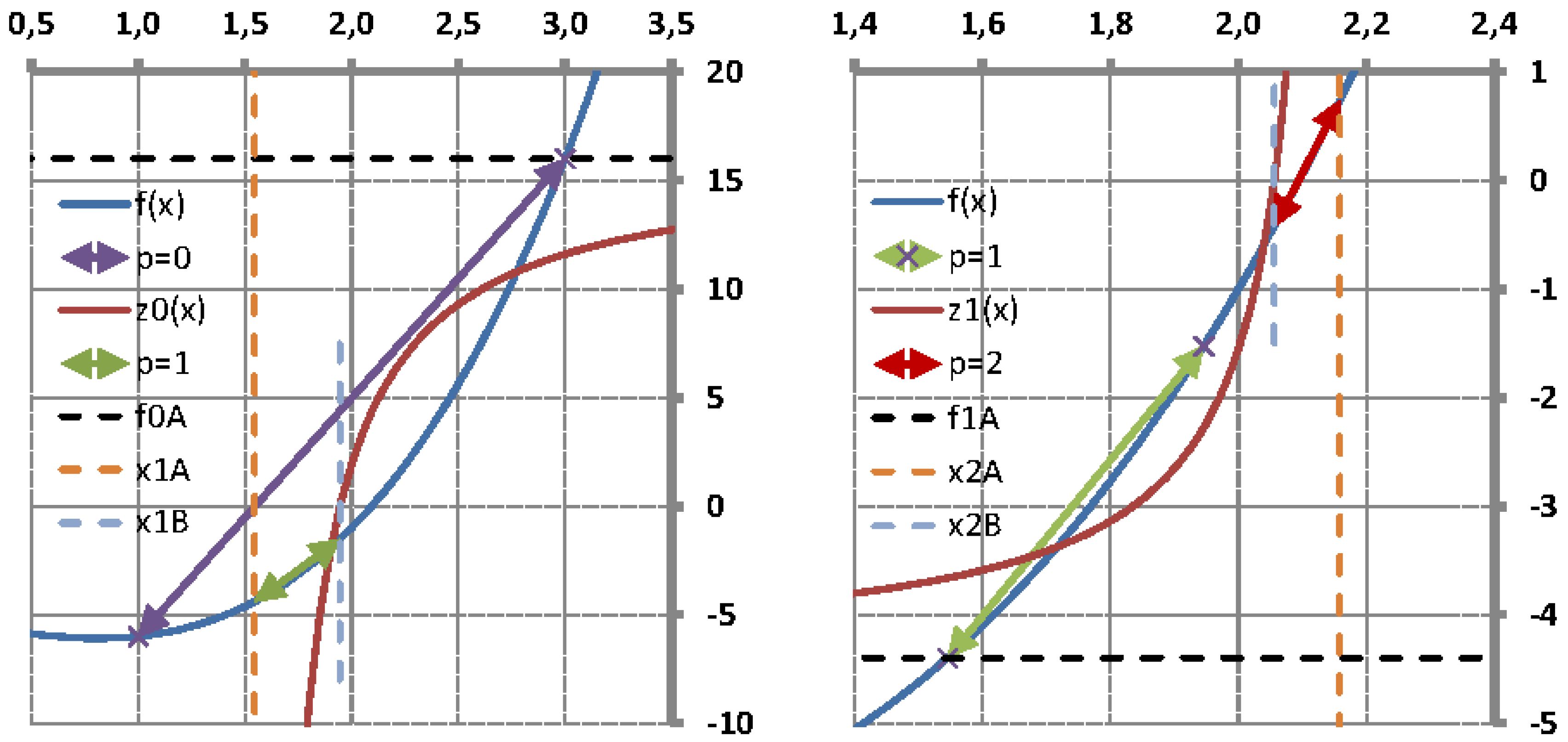
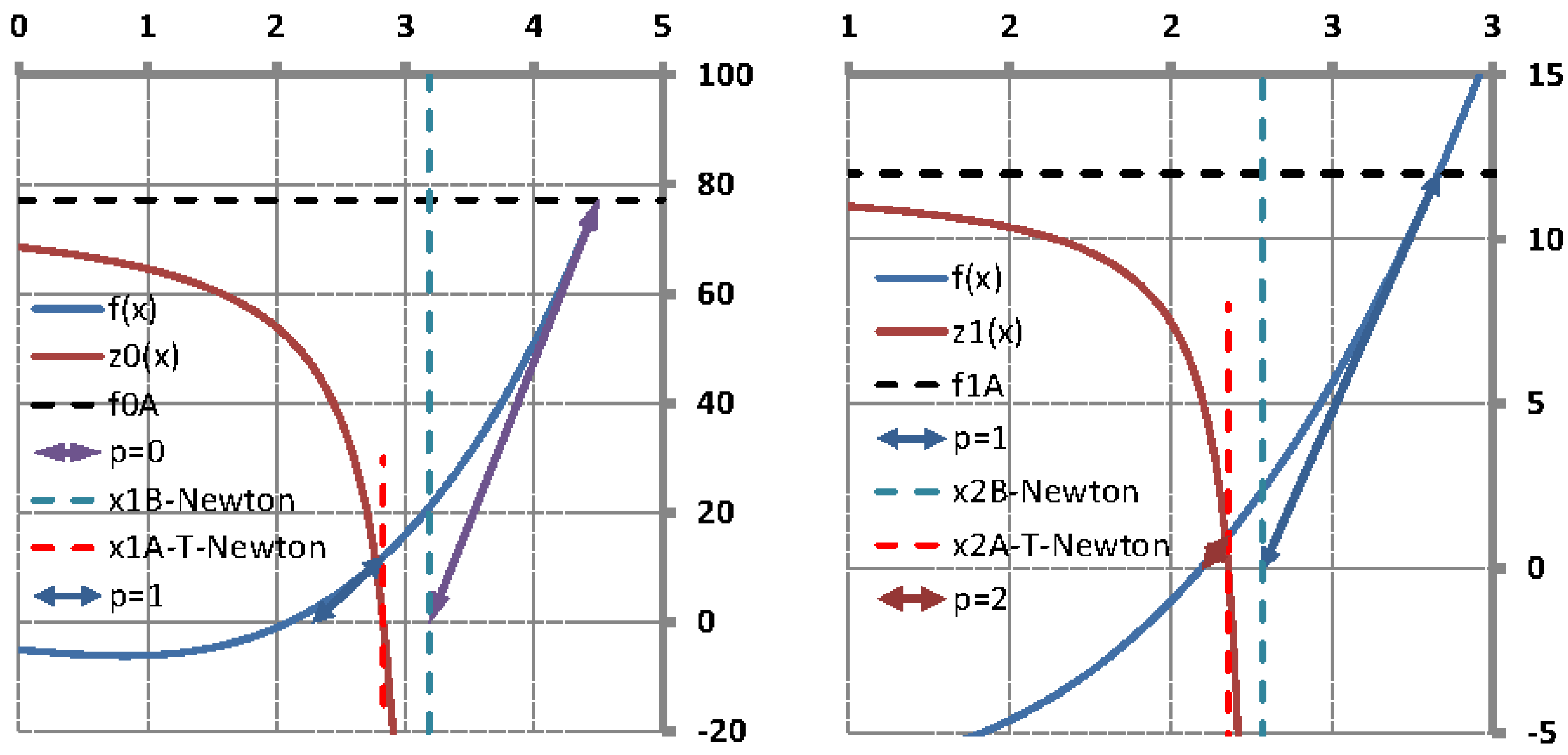
with root

x^{*} ≅ 2.09455 . . .

. Figure 4 summarizes the results of the first two iterations (left :

x_{1}^{A}

is the zero of

y_{0} (x)

x_{1}^{B}

is the zero of

z_{0} (x)

, right :

x_{2}^{A}

is the zero of

y_{1} (x)

x_{2}^{B}

is the zero of

z_{1} (x)

). Iterations were made with initial approximates

x_{0}^{A} = 3.0

and

x_{0}^{B} = 1.0

providing

f_{0}^{A} = 16

(

p = 0

). The first secant approximate

x_{1}^{A} = 1.545 . . .

is found as the zero of the first secant

y_{0} (x)

and the first T-secant appropriate

x_{1}^{B} = 1.945 . . .

is found as the zero of the first hyperbola function

z_{0} (x)

(Figure 4, left). Iteration then goes on (

p = 1

) with new interpolation base point

x_{1}^{A} = 1.545 . . .

and

x_{1}^{B} = 1.945 . . .

providing

f_{1}^{A} = - 4.3997 . . .

, and new approximates

x_{2}^{A} = 2.158 . . .

and

x_{2}^{B} = 2.0556 . . .

are found as the zeros of the second secant and the second hyperbola function

y_{1} (x)

and

z_{1} (x)

receptively (Figure 4, right). The next iteration (

p = 2

) will then continue with interpolation base point

x_{2}^{A} = 2.158 . . . . . .

and

x_{2}^{B} = 2.0556 . . .

and with

f_{2}^{A} = 0.7367 . . .

. The iterated values of

f_{p}^{A}

x_{p}^{A}

and

x_{p}^{B}

are also indicated on the diagrams. Further diagrams of this example are shown in Section 7.3.

6. General formulations

Re-ordering Equation (3.17) gives the general equation

▵ F ▵ X^{- 1} ▵ x^{A} = - f^{A}

(6.1)

of the secant method. The initial trials are constructed according to Equation (3.5) providing that

▵ X

is a diagonal matrix with elements

(▵ x_{i}) = (x_{i, i}^{B} - x_{i}^{A})

(i = 1, \dots, n)

. Let the “Jacobean-type” matrix of the Secant-method be defined as

S = ▵ F ▵ X^{- 1}

(6.2)

S = [\begin{matrix} \frac{f_{1, 1}^{B} - f_{1}^{A}}{x_{1, 1}^{B} - x_{1}^{A}} & \dots & \frac{f_{n, 1}^{B} - f_{1}^{A}}{x_{n, 1}^{B} - x_{1}^{A}} \\ ⋮ & ⋮ & ⋮ \\ \frac{f_{1, m}^{B} - f_{m}^{A}}{x_{1, 1}^{B} - x_{1}^{A}} & \dots & \frac{f_{n, m}^{B} - f_{m}^{A}}{x_{n, 1}^{B} - x_{1}^{A}} \end{matrix}] = [\begin{matrix} \frac{▵ f_{1, 1}}{▵ x_{1}} & \dots & \frac{▵ f_{n, 1}}{▵ x_{n}} \\ ⋮ & ⋮ & ⋮ \\ \frac{▵ f_{1, m}}{▵ x_{1}} & \dots & \frac{▵ f_{n, m}}{▵ x_{n}} \end{matrix}] = [\frac{▵ f_{k, j}}{▵ x_{i}}]

(6.3)

(i = 1, \dots, n)

(j = 1, \dots, m)

(k = 1, \dots, n)

and

S^{+} = ▵ X ▵ F^{+}

(6.4)

Then Equation (6.1) simplifies as

S ▵ x^{A} = - f^{A}

(6.5)

and

▵ x^{A} = - S^{+} f^{A}

(6.6)

The

i^{th}

element of the new approximate

x_{p + 1}^{A}

in the

p^{th}

iteration will then be

x_{p + 1, i}^{A} = x_{p, i}^{A} + ▵ x_{p, i}^{A} = x_{p, i}^{A} - \sum_{j = 1}^{m} (S_{p, i, j}^{+} f_{p, j}^{A})

(6.7)

(i = 1, \dots, n)

. It follows from the 1st row of Equation 4.15 of the T-Secant method, from Equation 4.13 and from the Definition 6.4 of

S^{+}

, that the

p^{th}

iteration step-size is

▵ x_{p}^{A} = - T_{p}^{X} S_{p}^{+} {(T_{p}^{F})}^{- 1} f_{p}^{A}

(6.8)

and

T_{p}^{F} S_{p} {(T_{p}^{X})}^{- 1} ▵ x_{p}^{A} = - f_{p}^{A}

(6.9)

Let the modified “Jacobean-type” matrix of the T-Secant-method be defined as

S_{p, T} = T_{p}^{F} S_{p} {(T_{p}^{X})}^{- 1}

(6.10)

S_{p, T} = [\begin{matrix} \frac{f_{p + 1, 1}^{A}}{f_{p, 1}^{A}} & 0 & 0 \\ 0 & ⋱ & 0 \\ 0 & 0 & \frac{f_{p + 1, m}^{A}}{f_{p, m}^{A}} \end{matrix}] [\begin{matrix} \frac{▵ f_{p, 1, 1}}{▵ x_{p, 1}} & \dots & \frac{▵ f_{p, n, 1}}{▵ x_{p, n}} \\ ⋮ & ⋮ & ⋮ \\ \frac{▵ f_{p, 1, m}}{▵ x_{p, 1}} & \dots & \frac{▵ f_{p, n, m}}{▵ x_{p, n}} \end{matrix}] [\begin{matrix} \frac{▵ x_{p, 1}^{A}}{▵ x_{p + 1, 1}} & 0 & 0 \\ 0 & ⋱ & 0 \\ 0 & 0 & \frac{▵ x_{p, n}^{A}}{▵ x_{p + 1, n}} \end{matrix}]

(6.11)

and in condensed form with general matrix elements (without the

p

index) :

S_{T} = T^{F} S {(T^{X})}^{- 1} = d i a g (t_{j}^{F}) [\frac{▵ f_{k, j}}{▵ x_{i}}] d i a g (\frac{1}{t_{i}^{X}}) = [\frac{t_{j}^{F}}{t_{i}^{X}} \frac{▵ f_{k, j}}{▵ x_{i}}]

(6.12)

(i = 1, \dots, n)

(j = 1, \dots, m)

(k = 1, \dots, n)

and

S_{T}^{+} = T^{X} S^{+} {(T^{F})}^{- 1}

(6.13)

Equations (6.8) and (6.9) then can be re-written as

▵ x^{A} = - S_{T}^{+} f^{A}

(6.14)

and

S_{T} ▵ x^{A} = - f^{A}

(6.15)

in a similar form like in case of the traditional secant method (Equations 6.6 and 6.5). The

i^{th}

element

x_{p + 1, i}^{B}

of the

2^{nd}

new approximate

x_{p + 1}^{B}

in the

p^{th}

iteration will then be

x_{p + 1, i}^{B} = x_{p + 1, i}^{A} + ▵ x_{p, i}^{B} = x_{p + 1, i}^{A} - \frac{{(▵ x_{p, i}^{A})}^{2}}{\sum_{j = 1}^{m} (S_{p, i, j}^{+} \frac{f_{p, j}^{A}}{t_{p, j}^{F}})}

(6.16)

where

t_{p, j}^{F} \neq 0

(j = 1, \dots, m)

and

(i = 1, \dots, n)

. Note, that the T-secant modification in the secant method “Jacobean-type” matrix 6.3 is made with multipliers

t_{p, j}^{F} = \frac{f_{p + 1, j}^{A}}{f_{p, j}^{A}}

and

t_{p, i}^{X} = \frac{▵ x_{p + 1, i}}{▵ x_{p, i}^{A}}

to the difference quantities

▵ f_{p, k, j}

and

▵ x_{p, i}

. The basic equations of the secant method and the T-secant method are summarized in Table 2 : rows 1-4 are the elements (matrix

T

) of the basic equations, row 5-6 are the explicit basic equations, row 7 : the Jacobean-type matrices, row 8-9 are the general formulations of the basic equations.

7. Convergence

7.1. Single-variable case

As it was shown in Section 4 (Equation (4.12)), the

p^{th}

iteration step length of the

2^{nd}

new approximate

x_{p + 1}^{B}

▵ x_{p + 1} = t_{p}^{f} ▵ x_{p}^{A}

(7.1)

The secant method is super-linear convergent, so the new approximate

x_{p + 1}^{A}

is expected to be a much better approximate to the solution

x^{*}

then the previous one (

x_{p}^{A}

). Thus

|f_{p + 1}^{A}| ⋘ |f_{p}^{A}|

(7.2)

and

|t_{p}^{f}| = |\frac{f_{p + 1}^{A}}{f_{p}^{A}}|

(7.3)

is expected to be a “small positive number”. It means, that the T-secant approximate

x_{p + 1}^{B}

will always be in the vicinity of the classic secant approximate

x_{p + 1}^{A}

and the approximate errors of the new approximates will be of similar order, providing that the solution

x^{*}

will evenly be surrounded by the 2 new trial approximates

x_{p + 1}^{A}

and

x_{p + 1}^{B}

7.2. Convergence rate

It is well known that the single-variable secant method has asymptotic convergence for sufficiently good initial approximates

x^{A}

and

x^{B}

f^{'} (x)

doesn’t vanish in

x \in [\begin{matrix} x^{A} & x^{B} \end{matrix}]

and

f^{″} (x)

is continuous at least in a neighborhood of the zero

x^{*}

. The super-linear convergence property has also been proved in different ways and it is known that the order of convergence

α^{S} = (1 + \sqrt{5}) / 2

with asymptotic error constant

C = {(\frac{1}{2} |\frac{f^{″} (ξ)}{f^{'} (ξ)}|)}^{\frac{1}{α}}

(7.4)

The order of convergence of the T-secant method is determined in this section. Let

p

be the iteration counter and the approximate error be defined in the

p^{th}

iteration as

e_{p} = x_{p} - x^{*}

(7.5)

It follows from Equation (3.21) and from Definition 7.5 that the error

e_{p + 1}^{A}

of the new secant approximate

x_{p + 1}^{A}

can be expressed as

e_{p + 1}^{A} = \frac{e_{p}^{A} f_{p}^{B} - e_{p}^{B} f_{p}^{A}}{f_{p}^{B} - f_{p}^{A}} = \frac{x_{p}^{B} - x_{p}^{A}}{f_{p}^{B} - f_{p}^{A}} \frac{f_{p}^{B} / e_{p}^{B} - f_{p}^{A} / e_{p}^{A}}{x_{p}^{B} - x_{p}^{A}} e_{p}^{A} e_{p}^{B}

(7.6)

It follows from the mean value theorem, that the first factor of right side of Equation (7.6) can be replaced with

1 / f^{'} (η_{p})

, where

η_{p} \in (x_{p}^{A}, x_{p}^{B})

, if

f (x)

is continuously differentiable on

(x_{p}^{A}, x_{p}^{B})

and

f^{'} (η_{p}) \neq 0

. Let the function

f (x)

be approximated around the root

x^{*}

by a

2^{nd}

order Taylor series expansion as

f_{p} = f (e_{p} + x^{*}) = f (x^{*}) + e_{p} f^{'} (x^{*}) + \frac{1}{2} {(e_{p})}^{2} f^{″} (ξ_{p})

(7.7)

where

ξ_{p} \in (x_{p}^{A}, x_{p}^{B}, x^{*})

in the remainder term. Since

f (x^{*}) = 0

, it follows from Equation (7.7) that

\frac{f_{p}}{e_{p}} = f^{'} (x^{*}) + \frac{1}{2} f^{″} (ξ_{p}) e_{p}

(7.8)

Substituting this expression to Equation (7.6), and since

e_{p}^{B} - e_{p}^{A} = x_{p}^{B} - x_{p}^{A}

we get

e_{p + 1}^{A} = \frac{1}{2} \frac{f^{″} (ξ_{p})}{f^{'} (η_{p})} \frac{e_{p}^{B} - e_{p}^{A}}{x_{p}^{B} - x_{p}^{A}} e_{p}^{A} e_{p}^{B} = C_{p} e_{p}^{A} e_{p}^{B}

(7.9)

and

C_{p} = \frac{1}{2} \frac{f^{″} (ξ_{p})}{f^{'} (η_{p})}

(7.10)

If the series

\{x_{p}^{A}\}

converges to

x^{*}

, then

ξ_{p}

and

η_{p}

\to x^{*}

with increasing iteration counter

p

, and

C_{p} \to \frac{1}{2} \frac{f^{″} (x^{*})}{f^{'} (x^{*})} = c o n s t a n t

(7.11)

It follows from Equation (4.11) with Definition 7.5 and from the mean value theorem (with

η_{p - 1} \in (x_{p - 1}^{A}, x_{p - 1}^{B})

, if

f (x)

is continuously differentiable on

(x_{p - 1}^{A}, x_{p - 1}^{B})

) that

x_{p}^{B} = x_{p}^{A} - {(\frac{x_{p}^{A} - x_{p - 1}^{A}}{f_{p - 1}^{A}})}^{2} f^{'} (η_{p - 1}) f_{p}^{A}

(7.12)

and the error

e_{p}^{B}

of the T-secant approximate

x_{p}^{B}

can be expressed as

e_{p}^{B} = e_{p}^{A} - {(\frac{e_{p}^{A} - e_{p - 1}^{A}}{f_{p - 1}^{A}})}^{2} f^{'} (η_{p - 1}) f_{p}^{A}

(7.13)

With the Taylor-series expansion 7.7 for

f_{p - 1}^{A}

and

f_{p}^{A}

, where

ξ_{p - 1} \in (x_{p - 1}^{A}, x_{p - 1}^{B}, x^{*})

and

ξ_{p} \in (x_{p}^{A}, x_{p}^{B}, x^{*})

in the remainder term, we get

e_{p}^{B} = e_{p}^{A} - e_{p}^{A} {(\frac{e_{p}^{A} - e_{p - 1}^{A}}{e_{p - 1}^{A}})}^{2} γ_{p}

(7.14)

where

γ_{p} = \frac{\frac{f^{'} (x^{*})}{f^{'} (η_{p - 1})} + \frac{1}{2} \frac{f^{″} (ξ_{p})}{f^{'} (η_{p - 1})} e_{p}^{A}}{{(\frac{f^{'} (x^{*})}{f^{'} (η_{p - 1})} + \frac{1}{2} \frac{f^{″} (ξ_{p - 1})}{f^{'} (η_{p - 1})} e_{p - 1}^{A})}^{2}}

(7.15)

and

f^{'} (η_{p - 1}) \neq 0

. If the series

\{x_{p}^{A}\}

converges to

x^{*}

, then with increasing iteration counter

p

ξ_{p}

ξ_{p - 1}

η_{p - 1}

\to x^{*}

and

e_{p}^{A}

e_{p - 1}^{A} \to 0

, implies that

\frac{f^{'} (x^{*})}{f^{'} (η_{p - 1})} \to \frac{f^{'} (x^{*})}{f^{'} (x^{*})} = 1

(7.16)

and

γ_{p} \to 1

. By substituting

e_{p}^{B}

(Equation (7.14)) into Equation (7.9) gives

e_{p + 1}^{A} = C_{p} e_{p}^{A} (e_{p}^{A} - e_{p}^{A} {(\frac{e_{p}^{A} - e_{p - 1}^{A}}{e_{p - 1}^{A}})}^{2} γ_{p})

(7.17)

and by re-arranging

e_{p + 1}^{A} = C_{p} e_{p}^{A} (γ_{p} {(e_{p}^{A})}^{2} \frac{2 e_{p - 1}^{A} - e_{p}^{A}}{{(e_{p - 1}^{A})}^{2}} + (1 - γ_{p}) e_{p}^{A})

(7.18)

with

\{x_{p}^{A}\}

converges to

x^{*}

γ_{p} \to 1

and the above equation simplifies as

e_{p + 1}^{A} = C_{p} e_{p}^{A} {(e_{p}^{A})}^{2} \frac{2 e_{p - 1}^{A} - e_{p}^{A}}{{(e_{p - 1}^{A})}^{2}}

(7.19)

It means that

e_{p + 1}^{A}

depends on

e_{p}^{A}

and

e_{p - 1}^{A}

, and by assuming an asymptotic convergence, a power law relationship

|e_{p + 1}^{A}| = C {|e_{p}^{A}|}^{α}

(7.20)

can be established, where

C

is the asymptotic error constant and

α

is the convergence rate or also called “convergence order” of the iterative method. It also follows from Equation (7.20), that

|e_{p}^{A}| = C {|e_{p - 1}^{A}|}^{α}

(7.21)

and

|e_{p - 1}^{A}| = {(\frac{|e_{p}^{A}|}{C})}^{\frac{1}{α}}

(7.22)

Let

E = |e_{p}^{A}|

be introduced for simplifying purpose, then it follows from Equations (7.17), (7.20), (7.21) and (7.22) that

E^{α} = \frac{C_{p}}{C} E^{3} \frac{2 {(\frac{E}{C})}^{\frac{1}{α}} - E}{{(\frac{E}{C})}^{\frac{2}{α}}}

(7.23)

where

C_{p}

and

C

are constants and if the series

\{x_{p}^{A}\}

converges to

x^{*}

, then with increasing iteration counter

p

E \to 0^{+}

. Taking the logarithms of both sides of Equation (7.23) and dividing by

lnE

gives

α = \frac{ln \frac{C_{p}}{C}}{ln E} + 3 - \frac{2}{α} \cdot \frac{ln (\frac{E}{C})}{ln E} + \frac{ln (2 {(\frac{E}{C})}^{\frac{1}{α}} - E)}{ln E}

(7.24)

\{x_{p}^{A}\}

series converges to

x^{*}

, then with increasing iteration counter

p

E \to 0^{+}

ln E \to - \infty

and

lim_{E \to 0^{+}} \frac{ln \frac{C_{p}}{C}}{ln E} = 0

(7.25)

lim_{E \to 0^{+}} ln (\frac{E}{C}) = lim_{E \to 0^{+}} (ln E - ln C) = ln E

(7.26)

lim_{E \to 0^{+}} \frac{ln (2 E^{\frac{1}{α}} - E)}{ln E} = \frac{1}{α}

(7.27)

and Equation (7.24) simplifies as

α - 3 + \frac{1}{α} = 0

(7.28)

with root (convergence rate of the T-Secant method) :

α^{T S} = \frac{3 + \sqrt{5}}{2} ≅ 2.618033988 \dots = α^{S} + 1 = φ^{2}

(7.29)

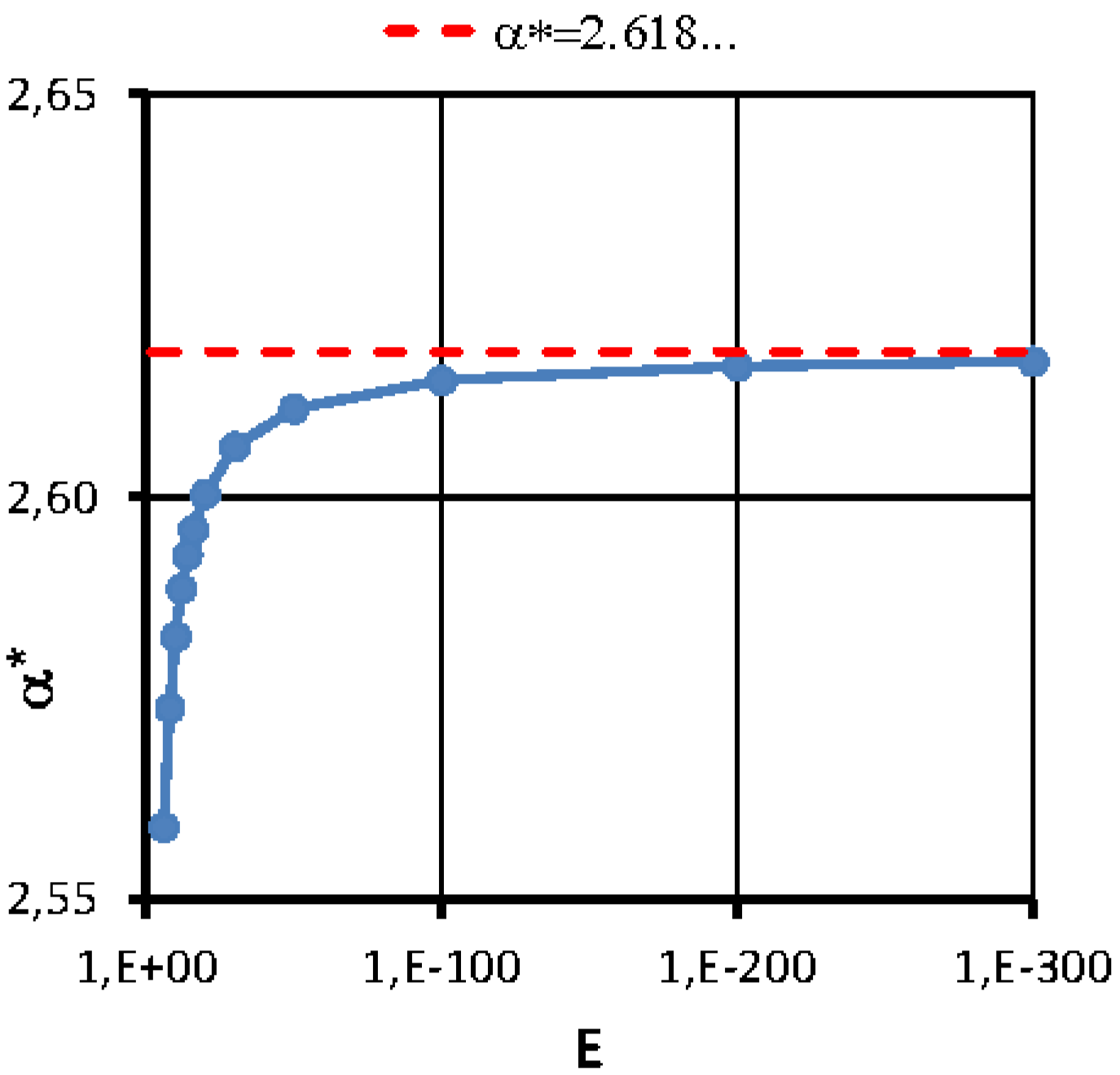
where

α^{S} = φ ≅ 1.618033988 \dots

is the convergence rate of the traditional secant method and ’ is the well known golden ratio. It follows from Equation (7.24) that the actual values

α^{*}

α^{T S}

depend on the approximate error

E = |e^{A}|

. Convergence rates

α^{*} (E)

were determined for different

E

values and shown on Figure 5. The upper bound

α^{T S} = α^{S} + 1 = 2.618 \dots

E \to 0^{+}

is also indicated (horizontal dashed red line).

7.3. Single-variable example

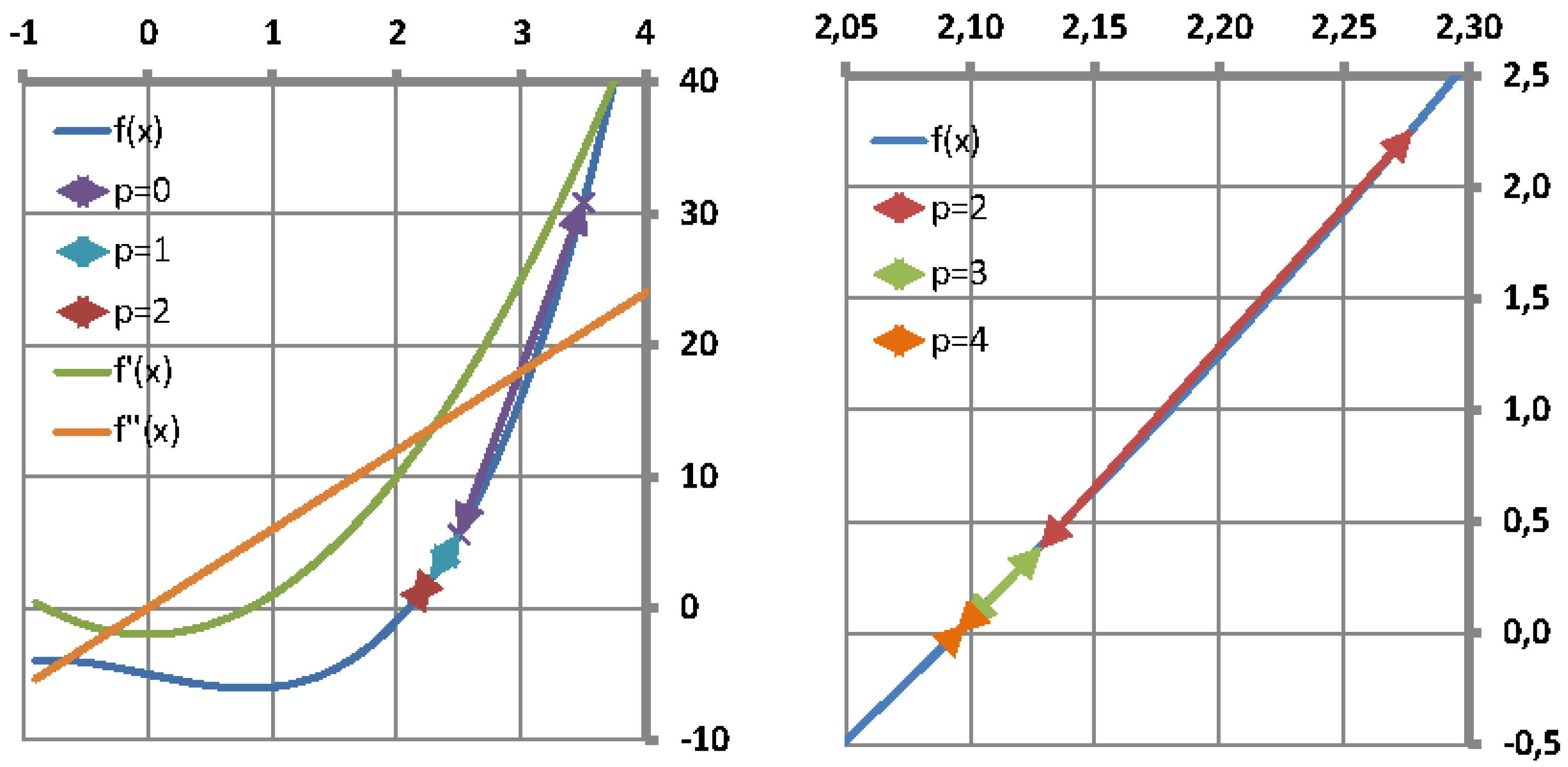
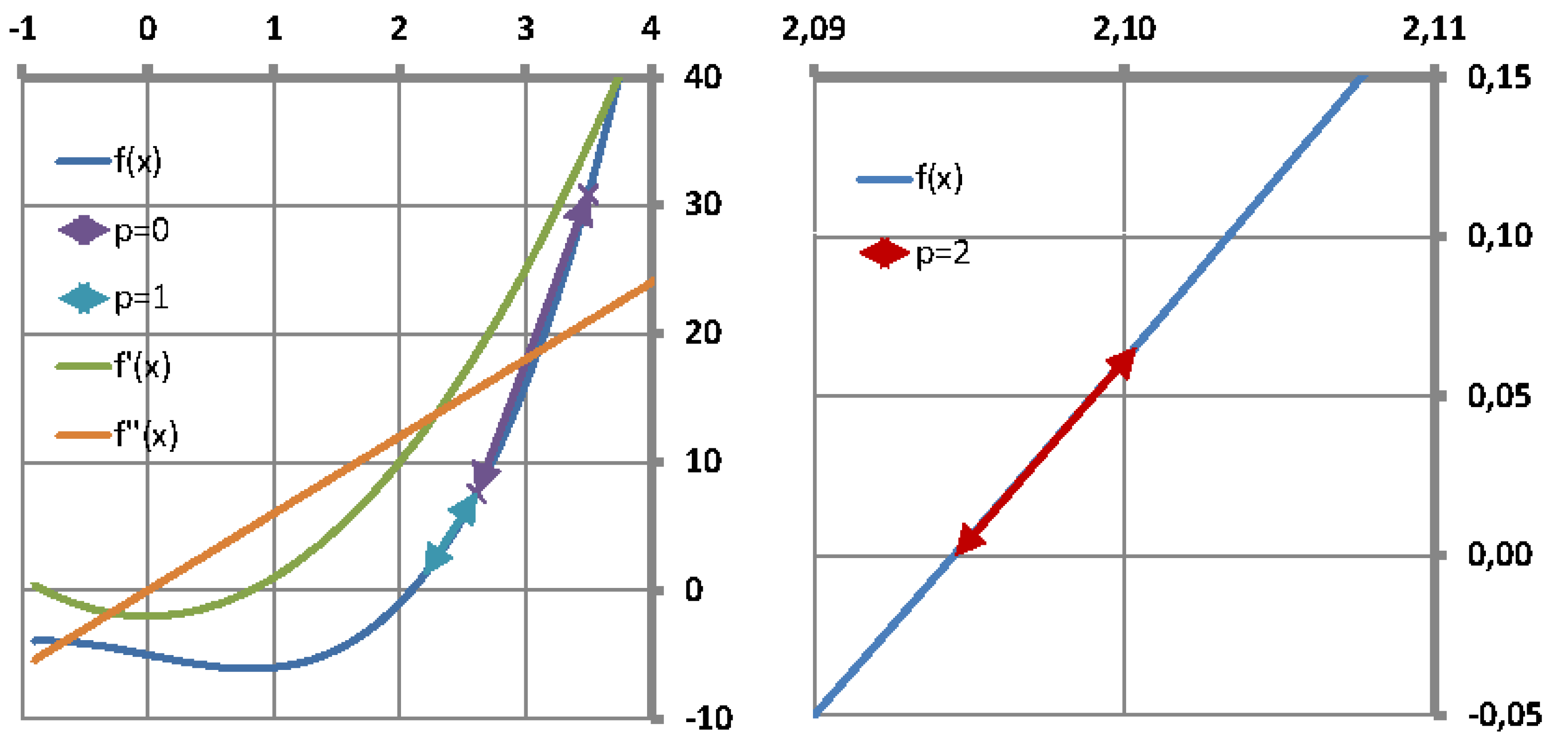
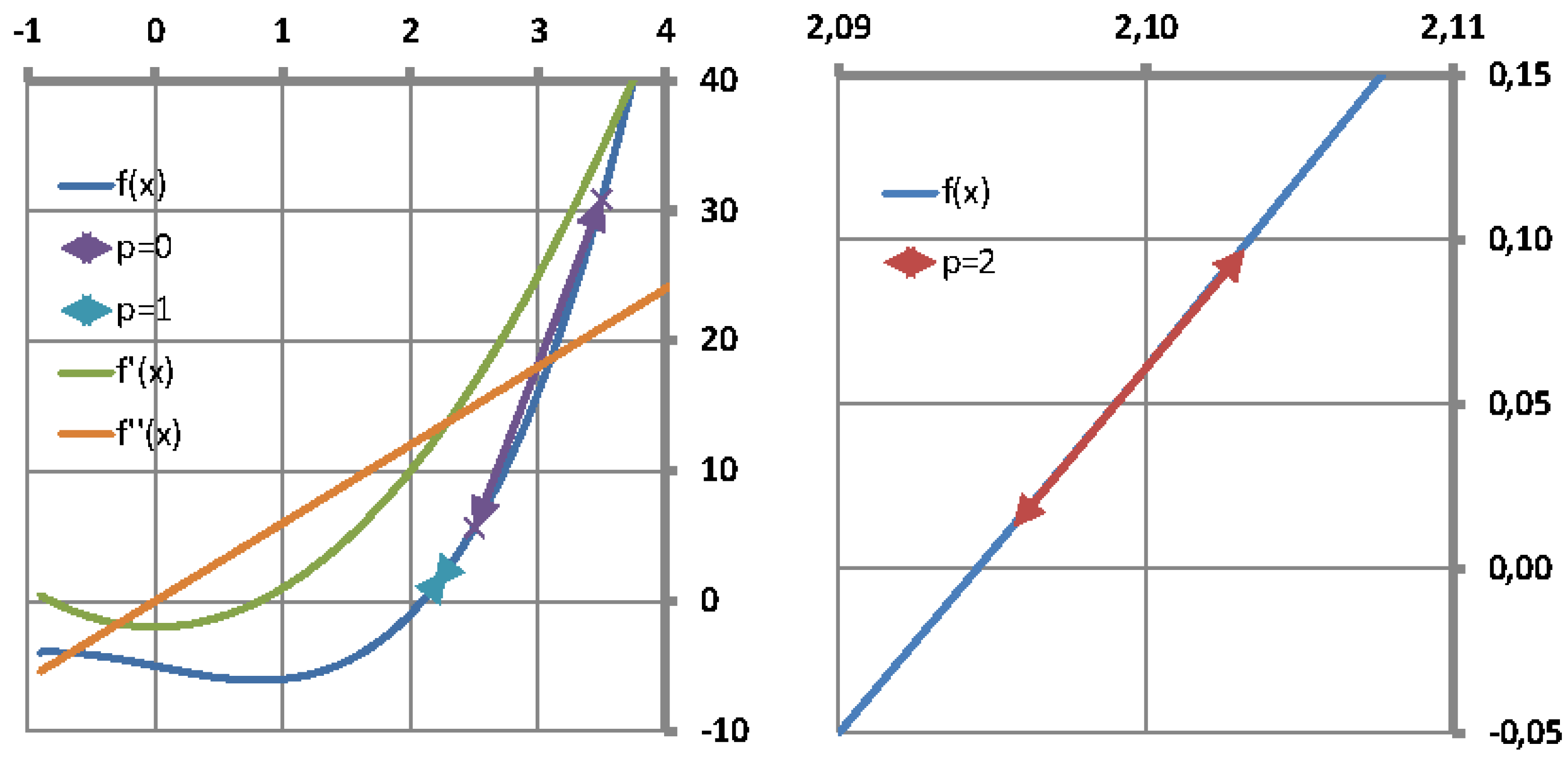
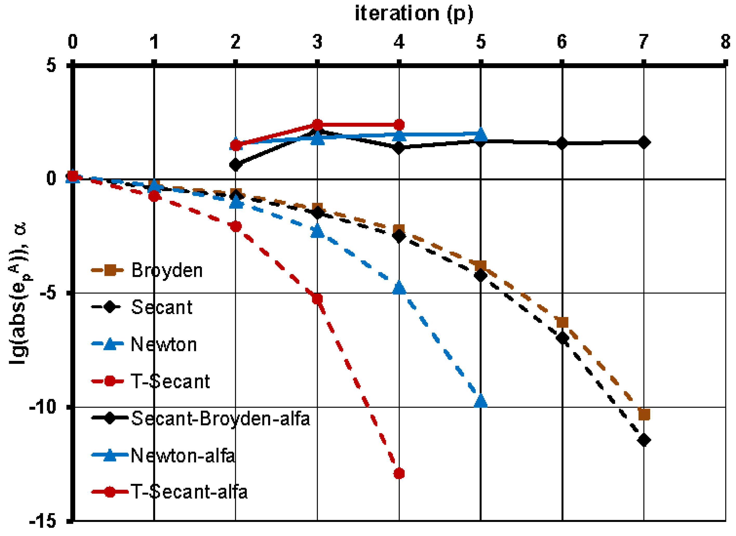
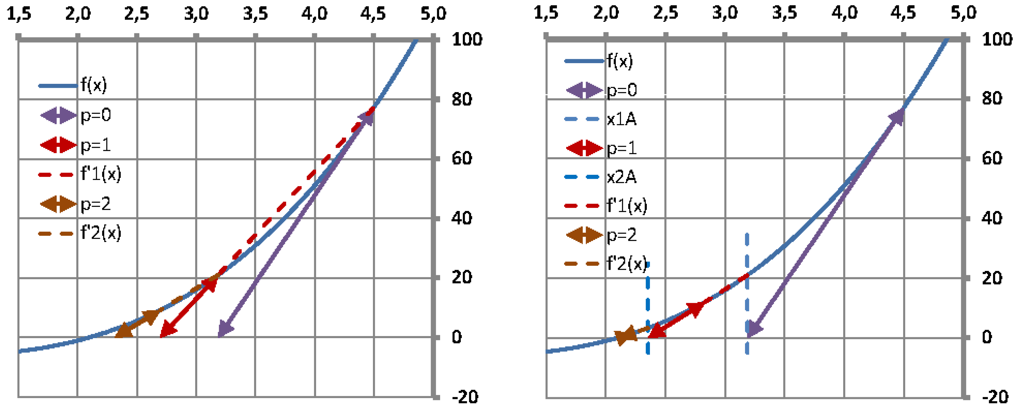
An example is given for demonstration purpose with a single-variable test function 5.26 with root

x^{*} ≅ 2.09455 . . .

. Iterations were made with initial approximates

x_{0}^{A} = 3.5

and

x_{0}^{B} = 2.5

and the convergence rates

α^{S}

α^{N}

and

α^{T S}

were determined for the traditional secant method (Table 3, Figure 6), for the Newton-Raphson method (Table 4, Figure 7) and for the T-secant method (Table 5, Figure 8) respectively, the cumulative number of function value (

N_{f}

) and derivative function value (

N_{f^{'}}

) calculations are also indicated in the tables. Calculated convergence rates agree well with theoretical values

α^{S} = 1.62 . . .

α^{N} = 2.0

and

α^{T S} = 2.62 . . .

. Figure 9 summarizes the results of iterations with three different methods (Secant, Newton-Raphson and T-Secant). Two groups of graphs show the absolute approximate error

|e_{p}^{A}|

decrease and the calculated convergence rates

α

for the three compared methods. Results demonstrate that the convergence rate of the T-Secant method is higher than the convergence rate of the Newton-Raphson method.

7.4. Multi-variable convergence

Matrix

S

corresponds to a divided difference approximation to the Jacobian. It is known (e. g. from Dennis-Schnabel [7]) that these values give a second order approximation to the derivative in the midpoint. When considering Newton’s iteration, it is assumed that the Jacobian has inverse in a neighbourhood of

x^{*}

. If that condition holds, than there are chances that the approximate Jacobian has also inverse in the same neighbourhood.

It follows from Equations (6.7) and (6.16), that the

i^{th}

elements of the iteration step lengths of the new approximates

x_{p + 1}^{A}

and

x_{p + 1}^{B}

in the

p^{th}

iteration are

▵ x_{p, i}^{A} = - \sum_{j = 1}^{m} (S_{p, i, j}^{+} f_{p, j}^{A})

(7.30)

and

▵ x_{p + 1, i} = - \frac{{(▵ x_{p, i}^{A})}^{2}}{\sum_{j = 1}^{m} (S_{p, i, j}^{+} \frac{f_{p, j}^{A}}{t_{p, j}^{F}})}

(7.31)

(i = 1 \dots, n)

. It is known, that the secant method is locally q-super-linear convergent, so the new approximate

x_{p + 1}^{A}

is expected to be a much better approximate to the solution

x^{*}

then the previous approximate

x_{p}^{A}

. Thus

∥f_{p + 1}^{A}∥ ⋘ ∥f_{p}^{A}∥

(7.32)

and the diagonal elements

|t_{p, j}^{F}| = |\frac{f_{p + 1, j}^{A}}{f_{p, j}^{A}}| ⋘ 1

(7.33)

of the transformation matrix

T_{p}^{F}

(j = 1 \dots, m)

are expected to be “small numbers”. Let the scalar multipliers

μ_{i}

be introduced so that

μ_{i} |\sum_{j = 1}^{m} (S_{p, i, j}^{+} \frac{f_{p, j}^{A}}{t_{p, j}^{F}})| = |\sum_{j = 1}^{m} (S_{p, i, j}^{+} f_{p, j}^{A})|

(7.34)

Then Expression 7.31 for the

i^{th}

element of the iteration step length

▵ x_{p + 1}

of the new approximate

x_{p + 1}^{B}

in the

p^{th}

iteration simplifies as

▵ x_{p + 1, i} = - \frac{{(▵ x_{p, i}^{A})}^{2}}{\frac{1}{μ_{i}} \sum_{j = 1}^{m} (S_{p, i, j}^{+} f_{p, j}^{A})} = μ_{i} \frac{{(▵ x_{p, i}^{A})}^{2}}{▵ x_{p, i}^{A}} = μ_{i} ▵ x_{p, i}^{A}

(7.35)

where

μ_{i} ⋘ 1

(7.36)

(i = 1 \dots, n)

and it follows from the above derivations that

∥▵ x_{p + 1}∥ \leq ∥μ∥ ∥▵ x_{p}^{A}∥

(7.37)

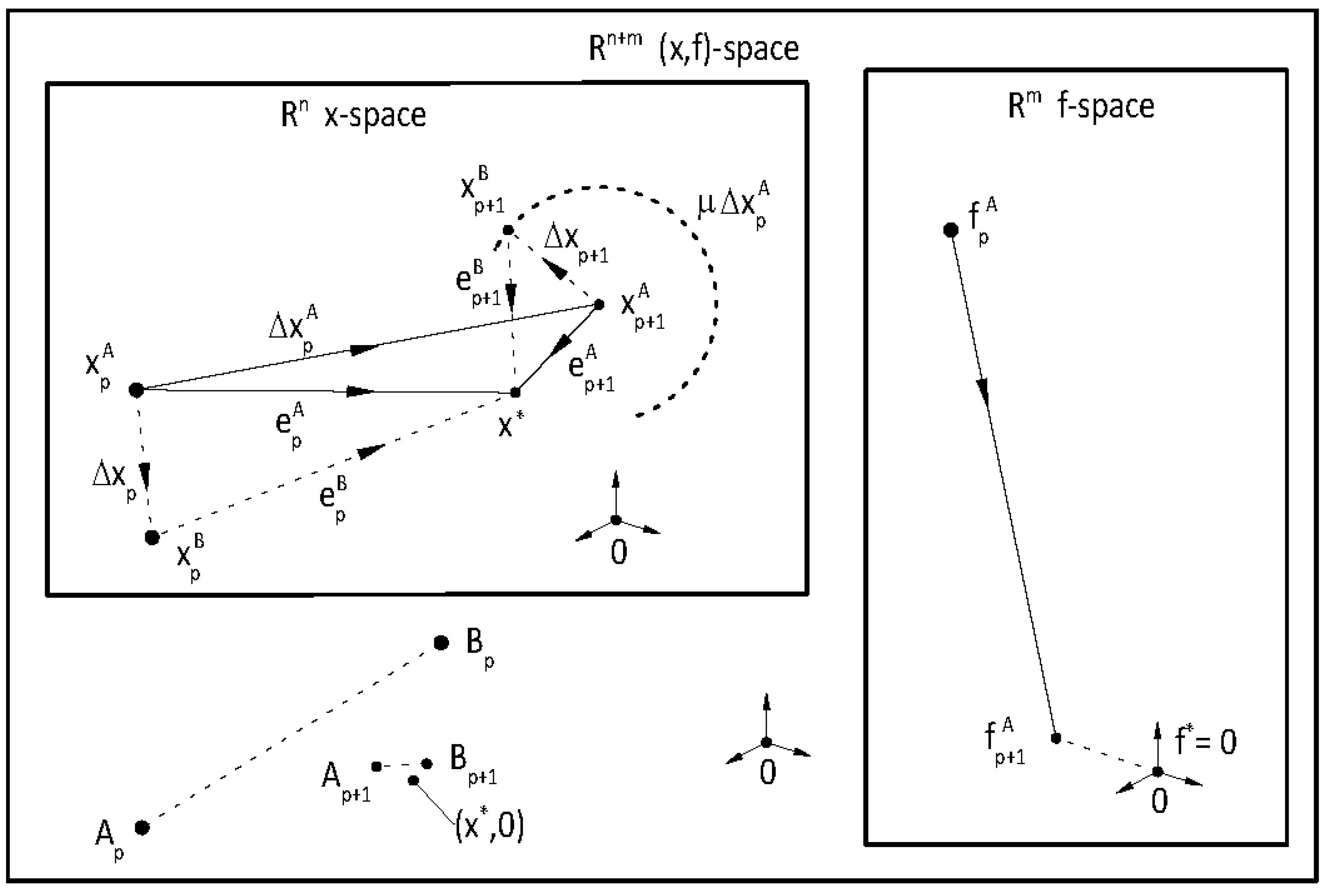
It means, that the T-secant approximate

x_{p + 1}^{B}

will always be in the vicinity of the classic secant approximate

x_{p + 1}^{A}

and the approximate errors of the new approximates will be of similar order, providing that the solution

x^{*}

will evenly be surrounded by the

n + 1

new trial approximates

x_{p + 1}^{A}

and

x_{k, p + 1}^{B}

(k = 1 \dots, n)

and matrix

S_{p + 1}

will be well-conditioned.

Figure 10. Geometrical representation of the T-secant method convergence in multi-variable case (analogous to the convergence proof figure Dennis-Schnabel [7], p. 180.).

8. Algorithm

Let

p

be the iteration counter,

ε^{*}

be the error bound for termination criterion and

e_{p}^{A} = x_{p}^{A} - x^{*}

(8.1)

be the approximate error vector of approximate

x^{A}

in the

p^{th}

iteration with elements

e_{p, i}^{A}

(i = 1, \dots, n)

. Let the scalar approximate error

ε_{p} = \frac{{∥e_{p}^{A}∥}_{2}}{n} = \frac{\sqrt{\sum_{i = 1}^{n} {(e_{p, i}^{A})}^{2}}}{n}

(8.2)

be defined, where

{∥\dots∥}_{2}

is Euclidean norm and let the iteration be terminated when

ε_{p} < ε^{*}

(8.3)

holds. Let

x_{p}^{A}

be the initial trial and

▵ x_{p}

be the trial increment in the

p^{t h}

iteration. Choose

T_{\min}

and

T_{\max}

as lower and upper bounds for

|t_{p, j}^{F}|

(j = 1 \dots, m)

and let

f_{\min}

and

q_{\min}

be lower bounds for

|f_{p, j}^{A}|

(j = 1, \dots, m)

and

|q_{p, i}^{B}|

(i = 1, \dots, n)

respectively.

Initial step

Let $p = 0$ and let the initial trial $x_{p}^{A} = (\begin{matrix} x_{p, 1}^{A} & \dots & x_{p, n}^{A} \end{matrix})$ and the initial trial increment $▵ x_{p} = (\begin{matrix} ▵ x_{p, 1} & \dots & ▵ x_{p, n} \end{matrix})$ be given. Calculate the corresponding function values $f_{p}^{A}$ and assume that $f_{\min} < |f_{p, j}^{A}| (j = 1 \dots, m)$ .
Step 1 : Generate a set of $n$ additional initial trials (interpolation base points)

$x_{p, k}^{B} = x_{p}^{A} + ▵ x_{p, k} \cdot d^{k}$

(8.4)

and evaluate function values $f_{p, k}^{B}$ $(k = 1, \dots, n)$ .
Step 2 (Secant) : Construct matrix

$▵ F_{p} = [▵ f_{p, k}^{i}] = [f_{p, k}^{B} - f_{p}^{A}]$

(8.5)

then calculate $q_{p}^{A}$ from Equation 3.15. Let $q_{\min} < |q_{p, i}^{A}|$ , and determine $x_{p + 1}^{A}$ from Equation (3.19) and $ε_{p}$ from Equation 8.2.
Step 3 : If $ε_{p}$ < $ε^{*}$ then terminate iteration, else continue with Step 4.
Step 4 (T-secant) : Calculate $f_{p + 1}^{A}$ and $T_{p}^{F}$ from Equation (4.19). Let $T_{\min} < |t_{p, j}^{F}| < T_{\max}$ and determine $q_{p}^{B}$ from Equation 4.20 ( $▵ F_{p}^{+}$ has already been calculated when $q_{p}^{A}$ was determined from Equation (3.15)). Let $q_{\min} < |q_{p, i}^{B}|$ , calculate $x_{p + 1}^{B}$ from Equation (4.22).
Step 5 : Let the new initial trial be

$v_{p + 1}^{A} = [\begin{matrix} x_{p + 1}^{A} \\ f_{p + 1}^{A} \end{matrix}]$

(8.6)

and the new initial trial increment be

$▵ x_{p + 1} = x_{p + 1}^{B} - x_{p + 1}^{A}$

(8.7)

and continue iteration with Step 1.

Iteration constants

(\begin{matrix} δ_{m i n} & f_{m i n} & q_{m i n} & T_{m i n} & T_{m a x} \end{matrix})

are necessary to avoid division by zero and to avoid computed values be near the numerical precision. If

p_{\max}

is the number of necessary iterations for satisfying the termination criterion

ε_{p} < ε^{*}

and

n

is the number of unknowns to be determined, then T-Secant method needs

n + 1

function evaluations in each iterations and altogether

N_{f} = p_{\max} (n + 1)

(8.8)

function evaluations to reach the desired termination criterion.

p_{\max}

is depending on many circumstances such as the nature of the function

f (x)

, termination criteria (

ε^{*}

or others), the distance of the initial trial

x^{A}

from the solution

x^{*}

and from the iteration constants

(T_{\min}, q_{\min}^{A}, \dots)

9. Numerical tests results

9.1. Rosenbrock test function

A variant of the Rosenbrock function [8] has been used for testing the numerical performance of the new method. Determine the global minimum of the function

R (x) = \sum_{i = 1}^{N - 1} (100 \cdot {(x_{i + 1} - x_{i}^{2})}^{2} + {(1 - x_{i})}^{2})

(9.1)

where

x = (\begin{matrix} x_{1} & \dots & x_{N} \end{matrix}) \in R^{N}

and

N \geq 2

R (x)

has exactly one minimum for

N = 3

x^{*} =

(\begin{matrix} 1 & 1 & 1 \end{matrix})

and exactly two minima for

4 \leq N \leq 7

, a global minimum of all ones and a local minimum near

\hat{x} = (\begin{matrix} - 1 & 1 & \dots & 1 \end{matrix})

. The sum of squares

R (x)

will be minimum when all terms are zero, such that the minimization of the function

R (x)

is equivalent with finding the zero of a function

x \to f (x)

, where

x \in R^{N}

f : R^{N} \to R^{2 (N - 1)}

, and

f (x) = [\begin{matrix} f_{2 i - 1} (x) \\ f_{2 i} (x) \end{matrix}] = [\begin{matrix} 10 \cdot (x_{i + 1} - x_{i}^{2}) \\ 1 - x_{i} \end{matrix}]

(9.2)

(i = 1, \dots, N - 1)

. For

N > 7

, the function

R (x)

has exactly one global minimum

x^{*} = (\begin{matrix} 1 & \dots & 1 \end{matrix})

and has some local minima with some

x_{j}^{*} = - 1

and with

x_{i}^{*} = 1

for all other unknowns. The results were obtained by least squares solving of the simultaneous system of nonlinear equations

f (x) = 0

by the T-Secant method.

9.2. $N = 2$ , $N = 3$ and $N = 10$ examples

In case

N = n = m = 2

, iterations terminated after

N_{f} = 6

function evaluations (

p_{\max} = 2

iterations) in most cases.

f_{2} (x) = 1 - x_{1}

is a linear function and the first T-secant iteration

(p = 0)

finds the exact value of

x_{1}

in one step, then

f_{1} (x) = 10 (x_{2} - x_{1}^{2})

also becomes linear. The exact value of

x_{2}

was then determined in one additional step.

Let

N = n = 3

and

m = 4

T_{\min} = 0.01

and

ε^{*} = 10^{- 14}

. Let

p = 0

, and

▵ x_{0, i} = 0.05 \cdot x_{0, i}^{A}

(9.3)

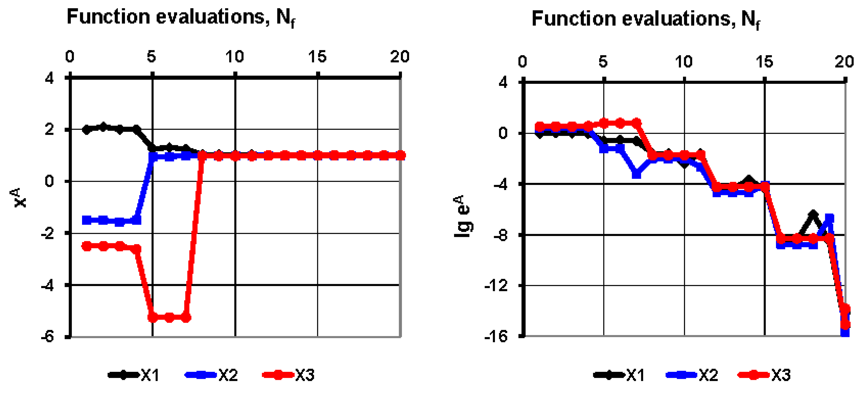
(i = 1 \dots, 3)

. The number of necessary function evaluations

N_{f}

varied between

20 - 36

within

p_{\max} = 5 - 9

iterations for different initial trials

x_{p}^{A}

. Iteration results are summarized in Table 6 and in Figure 11 with initial trial

x_{0}^{A} = (x_{0, i}^{A}) = (\begin{matrix} 2.0 & - 1.5 & - 2.5 \end{matrix})

. Termination criterion

ε_{p} < ”^{*}

was satisfied after

p_{\max} = 5

iterations with

N_{f} = 20

function evaluations.

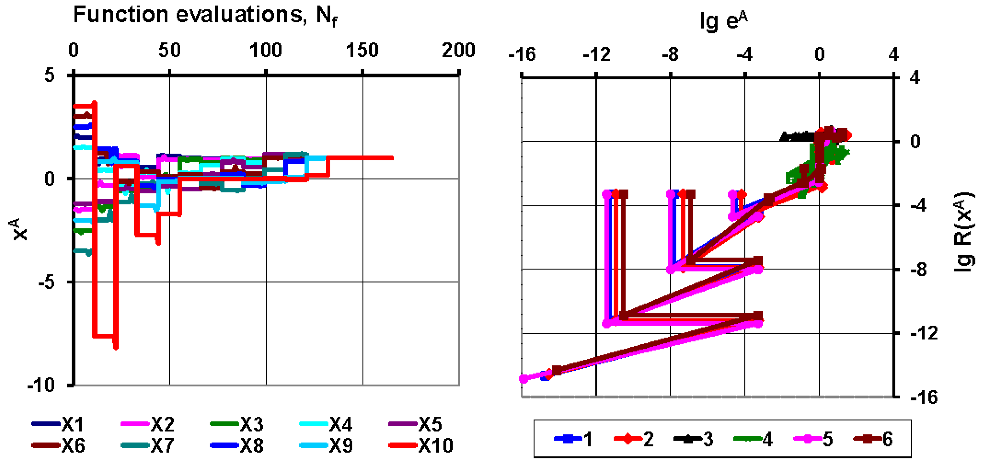
Let

N = n = 10

and

m = 18

. Calculations were made with different, manually constructed initial trials

x_{0}^{A} = (x_{0, i}^{A})

. Figure 12 (Left) shows the variation of

x_{p, i}^{A}

for initial trial

x_{0}^{A} = (\begin{matrix} 2.0 & - 1.5 & - 2.5 & 1.5 & - 1.2 & 3.0 & - 3.5 & 2.5 & - 2.0 & 3.5 \end{matrix})

. Iteration terminated after

N_{f} = 154

function evaluations (

p_{\max} = 14

iterations) for

ε_{p} < ε^{*} = 10^{- 14}

condition. Table 7 shows a set of further initial trials for numerical tests. Test “3” failed probably due to the large distance from the global optimal solution. Test “4” found a local zero

x^{*} = (\begin{matrix} - 1 & 1 & 1 & 1 & 1 & 1 & 1 & 1 & 1 & 1 \end{matrix})

. Figure 12 (Right) summarizes the results of numerical tests “1-6”. Graphs show the iteration paths in the

l g |e_{p}^{A}| - R_{p} (x_{p}^{A})

plane. They have an initial part where the variation of

R_{p} (x_{p}^{A})

seems “chaotic”, while below

|e_{p}^{A}| ≅ 0.01

and

R_{p} (x_{p}^{A}) ≅

0.001 the iterations run on similar paths.

9.3. Large $N (2005001000)$ examples

A series of numerical test has been performed with large number of unknown variables. The values of the initial trials

x_{0}^{A} = (x_{0, i}^{A}), (i = 1, \dots N)

were generated as

x_{0, i}^{A} = x_{i}^{*} + L_{1} \cdot \frac{R a n d o m - \frac{1}{2}}{5} + L_{2}

(9.4)

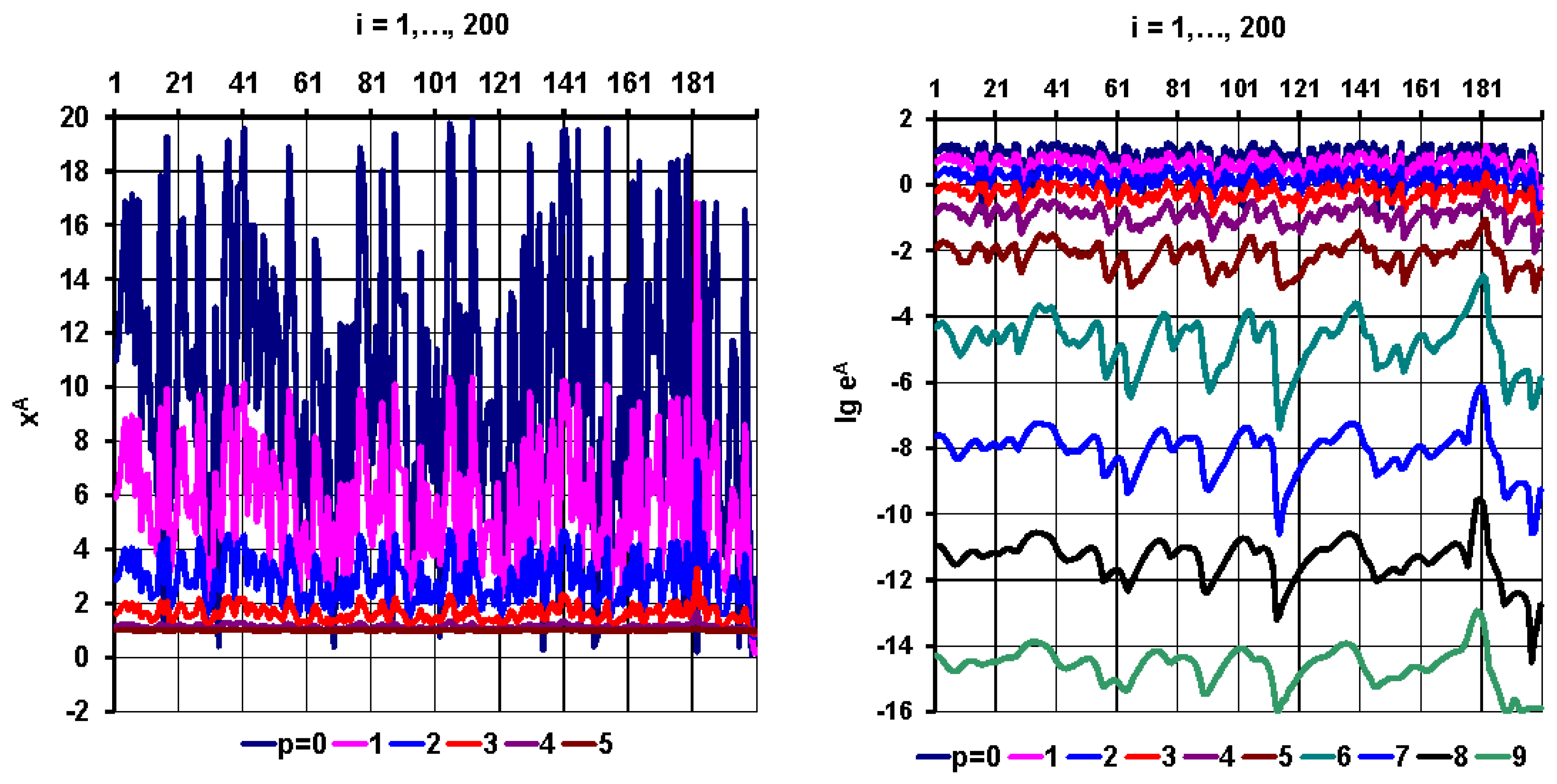
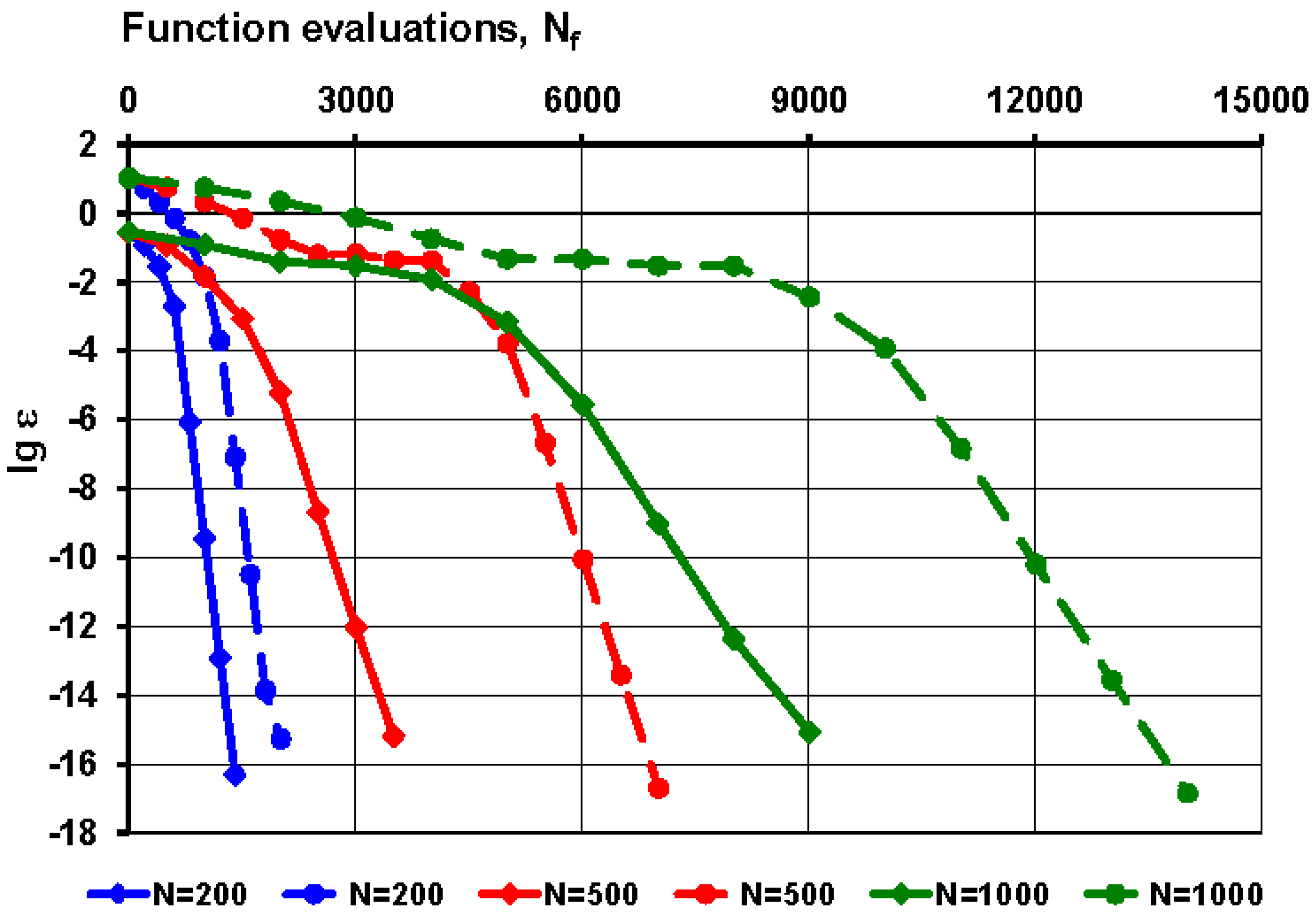
where “

Random

” is a random real number (

0 \leq Random < 1

L_{i} (i = 1, 2)

are parameters regulating the size and location of the interval in which the initial trial values are expected to variate.

x^{*} = (x_{i}^{*}) = (\begin{matrix} 1 & \dots & 1 \end{matrix}) (i = 1, \dots N)

is the known global optimal solution. Table 8 shows the results of T-Secant iterations with

N = 200

and with initial trials

x_{0}^{A} : 0.1 \leq x_{0, i}^{A} \leq 19.9

(

L_{1} = 99, L_{2} = 9

). Figure 13 (Left) shows the variation of variables

x_{p}^{A}

through T-Secant iterations. The iteration counter

p

value is indicated below the graphs for iterations. Figure 13 (Right) shows the decrease of the approximate error

e_{p}^{A} = (e_{p, i}^{A})

(i = 1, \dots, 200)

, with the

p

iteration counter indication below the graphs. Table 9 shows the results of iterations with

N = 1000

and initial trials

x_{0}^{A} : 0.5 \leq x_{0, i}^{A} \leq 1.5

(

L_{1} = 5, L_{2} = 0

). Figure 14 summarizes the results of numerical tests with large number of unknowns

N = (\begin{matrix} 200 & 500 & 1000 \end{matrix})

. The norm

ε_{p}

of the approximate error

e_{p}^{A}

decrease is shown and the number of function value evaluations

N_{f}

is indicated for

N = (\begin{matrix} 200 (b l u e) & 500 (r e d) & 1000 (g r e e n) \end{matrix})

and for initial trials

x_{0}^{A} : 0.5 \leq x_{0, i}^{A} \leq 1.5

(solid line) and

x_{0}^{A} : 0.1 \leq x_{0, i}^{A} \leq 19.9

(dashed line).

10. Efficiency

Very limited data are available to compare the performance of the T-secant method with other methods, especially for large number of unknowns. Broyden [9] suggested the mean convergence rate

L = \frac{1}{N_{f}} ln \frac{R (x_{0}^{A})}{R (x_{p_{m a x}}^{A})}

(10.1)

as a measure of efficiency of a method for solving a particular problem, where

N_{f}

is the total number of function evaluations,

x_{0}^{A}

is the initial trial,

x_{p_{\max}}^{A}

is the last trial for the solution

x^{*}

when the termination criteria is satisfied after

p_{\max}

iterations.

R (x)

is the Euclidean norm of

f (x)

. Efficiency results were given by Broyden [9] for the Rosenbrock function for

N = 2

and for

x_{0}^{A} = (\begin{matrix} - 1.2 & 1.0 \end{matrix})

. The calculated convergence rates for the two Broyden method variants [9], for the Powell’s method [10], for the adaptive coordinate descent method [11] and for the Nelder-Mead simplex method [12] were compared with the calculated values for the T-secant method in Table 10. Rows

1 - 5

are data from referenced papers, rows

6 - 8

are T-secant results with the referenced initial trials and rows 9-15 are calculated data for

N > 2

. Results show that the mean convergence rate

L

(Equation (10.1)) for

N = 2

is much higher for the T-secant method (

≃ 5.5 - 6.9

) than for the other listed methods (

≃ 0.1 - 0.6

), however it is obvious that the convergence rate values decrease rapidly with increasing

N

values (more unknowns need more function evaluations). A modified convergence rate

L_{N} = N * L = \frac{N}{N_{f}} ln \frac{R (x_{0}^{A})}{R (x_{p_{\max}}^{A})}

(10.2)

can be used as a more

” N ”

independent measure of efficiency (see Table 10) than the quantity

L

. The values of

L

and

L_{N}

are at least 10 times larger for the T-secant method than for the other listed methods for

N = 2

. Note that the efficiency measures (

L

and

L_{N}

) are also depending on the initial conditions (distance of the initial trial set from the optimal solution, termination criterion). Results from large number of numerical tests indicate an average

L_{N}

value around

7.4

with standard deviation

3.7

for the T-secant method even for large

N

values. It has to be noted that if the value of

R (x_{p_{\max}}^{A})

is zero, then the mean convergence rates (

L

and

L_{N}

) are not countable (zero in the denominator). A substitute value

10^{- 25}

was used when iteration ended with

R (x_{p_{\max}}^{A}) = 0

in the sample examples.

11. Discussions

11.1. General

The suggested new procedure needs the usual approximate

x_{p + 1}^{A}

be determined by any of a classic quasi-Newton iterative method (Wolfe-Popper-Secant, Broyden, etc.). By using the “information”

f (x_{p + 1}^{A}) = f_{p + 1}^{A}

, an additional and independent approximate

x_{p + 1}^{B}

is determined, that provides the possibility for a full-rank update of the exact or approximate derivatives (

S_{p}

for Secant or

B_{p}

for Broyden). Results and experience show that the new procedure considerably accelerates the convergence and the efficiency of the classic methods, and the full-rank update technique increases the stability of the iterative procedure. In multi-variable-case, it follows from Equation (6.8) that

{(T_{p}^{X})}^{- 1} ▵ x_{p}^{A} = - S_{p}^{+} {(T_{p}^{F})}^{- 1} f_{p}^{A}

(11.1)

and in explicit form after re-arrangement

[\frac{{(▵ x_{p, i}^{A})}^{2}}{x_{p + 1, i}^{B} - x_{p + 1, i}^{A}}] = - [S_{p, i, j}^{+}] [\frac{f_{p, j}^{A}}{t_{p, j}^{F}}]

(11.2)

Then the

i^{th}

element of the new approximate

x_{p + 1}^{B}

can be expressed from the

i^{th}

row of the above equation as

x_{p + 1, i}^{B} = x_{p + 1, i}^{A} - \frac{{(▵ x_{p, i}^{A})}^{2}}{\sum_{j = 1}^{m} (S_{p, i, j}^{+} \frac{f_{p, j}^{A}}{t_{p, j}^{F}})}

(11.3)

The mechanism of the procedure can be resembled to the mechanism of an engine’s turbocharger that is powered by the flow of exhaust gases (analogous to

f_{p + 1}^{A}

t_{p, j}^{F}

11.2. Newton method

Matrix

S

in the general formula 6.5 gives a direct connection between secant and Newton method, as differences go to differentials,

S = [\frac{▵ f_{k, j}}{▵ x_{i}}] = [S_{i, j}] ⟶ J = [\frac{\partial f_{k, j}}{\partial x_{i}}] = [J_{i, j}]

(11.4)

where

J

is the Jacobian matrix the function

f : R^{n} \to R^{m}

(

m \geq n

) with

k

and

i

column and with

j

row indeces respectively. It follows from formula 6.12 of matrix

S_{T}

that the proposed full-rank update procedure can also be applied to the Newton method as

S_{T} = [\frac{t_{j}^{F}}{t_{i}^{X}} \frac{▵ f_{k, j}}{▵ x_{i}}] ⟶ J_{T} = [\frac{t_{j}^{F}}{t_{i}^{X}} \frac{\partial f_{k, j}}{\partial x_{i}}]

(11.5)

where

J_{T}

is the modified Jacobian matrix of the ’T-Newton’ method. In single-variable case, with approximate

x_{p}^{A}

in the

p^{th}

iteration, with function value

f_{p}^{A} = f (x_{p}^{A})

and with derivative function value

f_{p}^{' A} = f^{'} (x_{p}^{A})

, the new Newton-Raphson approximate can be expressed as

x_{p + 1}^{A} = x_{p}^{A} - \frac{\partial x_{p}}{\partial f_{p}} f_{p}^{A} = x_{p}^{A} - \frac{f_{p}^{A}}{f_{p}^{' A}}

(11.6)

and the iteration step size is

▵ x_{p}^{A} = x_{p + 1}^{A} - x_{p}^{A}

(11.7)

With the hyperbolic function (Equation (5.15))

z_{p} (x) = \frac{a_{p}}{x - x_{p + 1}^{A}} + f_{p}^{A}

(11.8)

where

a_{p} = {(x_{p + 1}^{A} - x_{p}^{A})}^{2} f_{p}^{' A} \frac{f_{p + 1}^{A}}{f_{p}^{A}}

(11.9)

(

▵ f_{p} / ▵ x_{p}

is replaced by

f_{p}^{' A}

), the new ’T-Newton’ approximate is

x_{p + 1}^{B} = x_{p + 1}^{A} - \frac{{(▵ x_{p}^{A})}^{2} f_{p}^{' A} f_{p + 1}^{A}}{{(f_{p}^{A})}^{2}}

(11.10)

(

▵ f_{p} / ▵ x_{p}

is again replaced by

f_{p}^{' A}

) similarly like Equation (4.11) in case of the T-secant method. It can be seen from Table 11 and Table 12 that the convergence rate is be improved from

α^{N} = 2

α^{T N} = 3

. In multi-variable case, it follows from Equation (6.8) (

S_{p}^{+}

is replaced by

J_{p}^{+}

) that

{(T_{p}^{X})}^{- 1} ▵ x_{p}^{A} = - J_{p}^{+} {(T_{p}^{F})}^{- 1} f_{p}^{A}

(11.11)

and in explicit form after re-arrangement

[\frac{{(▵ x_{p, i}^{A})}^{2}}{x_{p + 1, i}^{B} - x_{p + 1, i}^{A}}] = - [J_{p, i, j}^{+}] [\frac{f_{p, j}^{A}}{t_{p, j}^{F}}]

(11.12)

Then the

i^{th}

element of the new the ’T-Newton’ approximate

x_{p + 1}^{B}

can be expressed from the

i^{th}

row of the above equation as

x_{p + 1, i}^{B} = x_{p + 1, i}^{A} - \frac{{(▵ x_{p, i}^{A})}^{2}}{\sum_{j = 1}^{m} (J_{p, i, j}^{+} \frac{f_{p, j}^{A}}{t_{p, j}^{F}})}

(11.13)

similarly like with Equation (4.22) in case of the T-secant method. Thus the “hyperbolic” approximation accelerates the convergence of the Newton-Raphson method by only one additional function evaluation.

11.3. Broyden’s method

Broyden’s method is a special case of the secant method. In single variable case, the derivative of the function is approximated as

f_{p}^{'} ≃ B_{p} = B_{p - 1} + \frac{▵ f_{p} - B_{p - 1} ▵ x_{p}}{{|▵ x_{p}|}^{2}} ▵ x_{p}

(11.14)

in the

p^{th}

iteration step, and with

\frac{▵ x_{p}}{{|▵ x_{p}|}^{2}} = \frac{1}{▵ x_{p}}

(11.15)

it is simplified as

B_{p} = B_{p - 1} + \frac{▵ f_{p} - B_{p - 1} ▵ x_{p}}{▵ x_{p}}

(11.16)

The next Broyden-approximate is then determined as

x_{p + 1}^{A} = x_{p}^{A} - \frac{f_{p}^{A}}{B_{p}}

(11.17)

The convergence can similarly be improved by the new hyperbolic approximation procedure as in cases of the secant and the Newton methods. An additional new approximate

x_{p + 1}^{B} = x_{p + 1}^{A} - \frac{{(▵ x_{p}^{A})}^{2} B_{p} f_{p + 1}^{A}}{{(f_{p}^{A})}^{2}}

(11.18)

can be determined, and the iteration continues with this value. Figure 16 demonstrates the effect of the hyperbolic approximation applied to the classic Broyden method. Not surprisingly, the convergence rate will be improved from

{f f}^{B} = φ ≃ 1.618

{f f}^{TB} = φ^{2} ≃ 2.618

as in case of the Secant method. In multi-variable case, the

i^{th}

element of the new the ’T-Broyden’ approximate

x_{p + 1}^{B}

can be expressed as

x_{p + 1, i}^{B} = x_{p + 1, i}^{A} - \frac{{(▵ x_{p, i}^{A})}^{2}}{\sum_{j = 1}^{m} (B_{p, i, j}^{+} \frac{f_{p, j}^{A}}{t_{p, j}^{F}})}

(11.19)

similarly like from Equation (11.13) in case of the T-Newton method with

J_{p, i, j}^{+}

replaced by

B_{p, i, j}^{+}

. The new approximate

B_{p + 1}

to the Jacobian matrix can then fully be updated in a similar way as it was shown in case of the T-secant method.

12. Conclusions

A completely new iteration strategy has been worked out for solving simultaneous nonlinear equations

f (x) = 0

(12.1)

x \in

R^{n}

and

f : R^{n} \to R^{m}

(

m \geq n

). It replaces the Jacobian matrix with finite-difference approximations. The step size

▵ x_{p + 1}

was determined as the difference between two new approximates

x_{p + 1}^{A} = x_{p}^{A} + ▵ x_{p}^{A}

(12.2)

and

x_{p + 1}^{B}

with elements

x_{p + 1, i}^{B} = x_{p + 1, i}^{A} + ▵ x_{p + 1, i} = x_{p + 1, i}^{A} - \frac{{(▵ x_{p, i}^{A})}^{2}}{\sum_{j = 1}^{m} (S_{p, i, j}^{+} \frac{f_{p, j}^{A}}{t_{p, j}^{F}})}

(12.3)

(i = 1, \dots, n)

▵ x_{p + 1} = x_{p + 1}^{B} - x_{p + 1}^{A}

(12.4)

The first one is a classic quasi-Newton approximate with stepsize

▵ x_{p}^{A}

, while the second one was determined from a hyperbolic approximation governed by

x_{p + 1}^{A}

and

f_{p + 1}^{A}

, such that the classic secant equation

S ▵ x^{A} = - f^{A}

(12.5)

was modified by a non-uniform scaling transformation

T = [\begin{matrix} T^{X} & 0 \\ 0 & T^{F} \end{matrix}]

(12.6)

with diagonal elements

t_{j}^{F}

(j = 1, \dots, m)

t_{i}^{X}

(i = 1, \dots, n)

S_{T} ▵ x^{A} = - f^{A}

(12.7)

where

S = [\frac{▵ f_{k, j}}{▵ x_{i}}] and S_{T} = [\frac{t_{j}^{F}}{t_{i}^{X}} \frac{▵ f_{k, j}}{▵ x_{i}}]

(12.8)

(k = 1, \dots, n)

. It was shown, that the new step size

▵ x_{p + 1}

is much smaller than the step size

▵ x_{p}^{A}

of the classic quasi-Newton approximate, providing that

x_{p + 1}^{B}

will always be in the vicinity of

x_{p + 1}^{A}

. Having two new approximates, a set of

n + 1

new independent trial approximates

x_{p + 1}^{A}

and

x_{k, p + 1}^{B}

(k = 1, \dots, n)

was constructed (see Equation (3.5)), providing that the new trial approximates are always in general positions, and ensures stable behavior of the iteration. According to the geometrical representation in single variable case, the suggested procedure corresponds to finding the root of a hyperbolic function with vertical and horizontal asymptotes

x_{p + 1}^{A}

and

f_{p}^{A}

. It was shown in Section 7 that the proposed method has super-quadratic convergence with rate

α^{T S} =

φ^{2} = 2.618 . . .

(where

φ = 1.618 . . .

is the well-known golden ratio) in single variable case. The proposed method needs two function evaluations in each iteration in single variable case and

n +

1 evaluations in multi-variable case. The efficiency of the proposed method was studied in Section 10 in multi-variable case and compared with other classic rank-one update and line-search methods on the basis of available test data. Results show, that the efficiency of the proposed full-rank update procedure is considerably better, then the efficiency of other classic low-rank update methods. A Rosenbrock test function (Equations (9.1) and (9.2)) with up to

n = 1000

variables was used to demonstrate the efficiency in Section 9.

Data Availability Statement

No new data were created or analyzed in this study. Data sharing is not applicable to this article.

Acknowledgments

A considerable part of the research work has been done between years 1988 -1992 at Technical University of Budapest (Hungary), at TNO-BOUW Structural Division (The Netherlands) and at Technical High-school of Lulea (Sweden). The work has been sponsored by the Technical University of Budapest (Hungary), by the Hungarian Academy of Sciences (Hungary), by TNO-BOUW (The Netherlands), by Sandvik Rock Tools (Sweden), by CP Test a/s (Denmark) and by Óbuda University (Hungary). Valuable discussions and personal supports from Géza Petrasovits, György Popper, Peter Middendorp, Rikard Skov, Bengt Lundberg and Csaba Hegedűs are greatly appreciated.

Conflicts of Interest

The author declares no conflict of interest.

References

Martínez, J.M. Practical quasi-Newton methods for solving nonlinear systems. Journal of Computational and Applied Mathematics. 2000, 124, 97–121. [Google Scholar] [CrossRef]
Wolfe, P. The Secant Method for Simultaneous Nonlinear Equations. Communications of the ACM. 1959, 2, 12–13. [Google Scholar] [CrossRef]
Popper, G. Numerical method for least square solving of nonlinear equations. Periodica Polytechnica. 1985, 29, 67–69. [Google Scholar]
Ortega, J.M.; Rheinboldt, W.C. Iterative Solution of Nonlinear Equations in Several Variables; Academic Press: New York, 1970. [Google Scholar]
Berzi, P. Model investigation for pile bearing capacity prediction. Euromech (280) Symposium on Identification of Nonlinear Mechanical Systems from Dynamic Tests, Ecully, 1991.
nal Berzi, P.; Beccu, R.; Lundberg, B. Identification of a percussive drill rod joint from its response to stress wave loading. International Journal of Impact Engineering. 1994, 18, 281–290. [Google Scholar] [CrossRef]
Dennis, J.E., Jr.; Schnabel, R.B. Numerical Methods for Unconstrained Optimization and Nonlinear Equations; Prentice-Hall: Englewood Cliffs, NJ, 1983. [Google Scholar]
Rosenbrock, H.H. An automatic Method for finding the Greatest or Least Value of a Function. The Computer Journal. 1960, 3, 175–184. [Google Scholar] [CrossRef]
Broyden, C.G. A class of Methods for Solving Nonlinear Simultaneous Equations. Mathematics of Computation. American Mathematical Society. 1965, 19, 577–593. [Google Scholar] [CrossRef]
Powell, M.J.D. An efficient method for finding the minimum of a function of several variables without calculating derivatives. Computer Journal. 1964, 7, 155–162. [Google Scholar] [CrossRef]
Loshchilov, I.; Schoenauer, M.; Sebag, M. Adaptive Coordinate Descent. Genetic and Evolutionary Computation Conference (GECCO), ACM Press, 885-892, 2011. [CrossRef]
Nelder, J.A.; Mead, R. A simplex method for function minimization. Computer Journal. 1965, 7, 308–313. [Google Scholar] [CrossRef]

Figure 1. Formulation of a new set of base vectors

(n = 3)

x^{A}

x_{1}^{B}

x_{2}^{B}

x_{3}^{B}

and interpolation base points

A

B_{1}

B_{2}

and

B_{3}

from new approximate

x^{A}

and from new trial increment

▵ x = x^{B} - x^{A} = {[\begin{matrix} ▵ x_{1} & ▵ x_{2} & ▵ x_{3} \end{matrix}]}^{T}

Figure 1. Formulation of a new set of base vectors

(n = 3)

x^{A}

x_{1}^{B}

x_{2}^{B}

x_{3}^{B}

and interpolation base points

A

B_{1}

B_{2}

and

B_{3}

from new approximate

x^{A}

and from new trial increment

▵ x = x^{B} - x^{A} = {[\begin{matrix} ▵ x_{1} & ▵ x_{2} & ▵ x_{3} \end{matrix}]}^{T}

Figure 2. Geometrical representation of the secant method in single-variable case (A : classic secant method, B : T-secant modification).

Figure 3. Vector space description of the T-secant method in multi-variable case (

k = 1, \dots n

Figure 3. Vector space description of the T-secant method in multi-variable case (

k = 1, \dots n

Figure 4. T-Secant iterations with test function 5.26 with initial approximates

x_{0}^{A} = 3.0

and

x_{0}^{B} = 1.0

(

Left

x_{1}^{A}

is the root of

y_{0} (x)

x_{1}^{B}

is the root of

z_{0} (x)

Right

x_{2}^{A}

is the root of

y_{1} (x)

x_{2}^{B}

is the root of

z_{1} (x)

Figure 4. T-Secant iterations with test function 5.26 with initial approximates

x_{0}^{A} = 3.0

and

x_{0}^{B} = 1.0

(

Left

x_{1}^{A}

is the root of

y_{0} (x)

x_{1}^{B}

is the root of

z_{0} (x)

Right

x_{2}^{A}

is the root of

y_{1} (x)

x_{2}^{B}

is the root of

z_{1} (x)

Figure 5.

α^{*}

convergence rate variation with decreasing

E \to 0^{+}

(dashed red lines indicate

α = α^{S} + 1 ≅ 2.618

level, where

α^{S} ≅ 1.618

is the convergence rate of the traditional secant method).

Figure 5.

α^{*}

convergence rate variation with decreasing

E \to 0^{+}

(dashed red lines indicate

α = α^{S} + 1 ≅ 2.618

level, where

α^{S} ≅ 1.618

is the convergence rate of the traditional secant method).

Figure 6. Secant iteration with test function 5.26 with initial approximates

x_{0}^{A} = 3.5

and

x_{0}^{B} = 2.5

(

Left

p = 0, 1,

2 ,

Right

p = 2, 3, 4

(see data in Table 3).

Figure 6. Secant iteration with test function 5.26 with initial approximates

x_{0}^{A} = 3.5

and

x_{0}^{B} = 2.5

(

Left

p = 0, 1,

2 ,

Right

p = 2, 3, 4

(see data in Table 3).

Figure 7. Newton iteration with test function 5.26 with initial approximate

x_{0}^{A} = 3.5

(

Left

p = 0, 1

Right

p = 2

(see data in Table 4).

Figure 7. Newton iteration with test function 5.26 with initial approximate

x_{0}^{A} = 3.5

(

Left

p = 0, 1

Right

p = 2

(see data in Table 4).

Figure 8. T-Secant iteration with test function 5.26 with initial approximates

x_{0}^{A} = 3.5

and

x_{0}^{B} = 2.5

(

Left

p = 0

(with interpolation base points

A_{0}

B_{0}

) and

p = 1

(

A_{1}

B_{1}

) ,

Right

p = 2

(

A_{2}

B_{2}

) (see data in Table 5).

Figure 8. T-Secant iteration with test function 5.26 with initial approximates

x_{0}^{A} = 3.5

and

x_{0}^{B} = 2.5

(

Left

p = 0

(with interpolation base points

A_{0}

B_{0}

) and

p = 1

(

A_{1}

B_{1}

) ,

Right

p = 2

(

A_{2}

B_{2}

) (see data in Table 5).

Figure 9. Absolute approximate error

|e_{p}^{A}|

decrease (dashed lines) and computed convergence rates (

α

) (solid lines) of different methods (Broyden (brown line), Secant (black lines), Newton-Raphson (blue lines), T-Secant (red lines) method).

Figure 9. Absolute approximate error

|e_{p}^{A}|

decrease (dashed lines) and computed convergence rates (

α

) (solid lines) of different methods (Broyden (brown line), Secant (black lines), Newton-Raphson (blue lines), T-Secant (red lines) method).

Figure 11.

(Left)

Variables

x_{p, i}^{A}

and

(Right)

absolute approximate errors

\lg |e_{p}^{A} (x_{p, i}^{A})|

(i = 1 . . . . 3)

variation for initial trial

x_{0}^{A} = (\begin{matrix} 2.0 & - 1.5 & - 2, 5 \end{matrix})

Figure 11.

(Left)

Variables

x_{p, i}^{A}

and

(Right)

absolute approximate errors

\lg |e_{p}^{A} (x_{p, i}^{A})|

(i = 1 . . . . 3)

variation for initial trial

x_{0}^{A} = (\begin{matrix} 2.0 & - 1.5 & - 2, 5 \end{matrix})

Figure 12.

(Left)

Variation of

x_{p, i}^{A}

for

x_{0}^{A} = (\begin{matrix} 2.0 & - 1.5 & - 2.5 & 1.5 & - 1.2 & 3.0 & - 3.5 & 2.5 & - 2.0 & 3.5 \end{matrix})

through iterations

(N = 10 = n = 10, m = 18)

with

p_{\max} = 15

and

N_{f} = 165

(Right)

The absolute approximate errors

\lg |e_{p}^{A} (x_{p, i}^{A})|

(i = 1 . . . . 10)

and the

R (x_{p}^{A})

function variation through iterations for different initial trials

(N = 10, n = 10, m = 18)

(see Table 7).

Figure 12.

(Left)

Variation of

x_{p, i}^{A}

for

x_{0}^{A} = (\begin{matrix} 2.0 & - 1.5 & - 2.5 & 1.5 & - 1.2 & 3.0 & - 3.5 & 2.5 & - 2.0 & 3.5 \end{matrix})

through iterations

(N = 10 = n = 10, m = 18)

with

p_{\max} = 15

and

N_{f} = 165

(Right)

The absolute approximate errors

\lg |e_{p}^{A} (x_{p, i}^{A})|

(i = 1 . . . . 10)

and the

R (x_{p}^{A})

function variation through iterations for different initial trials

(N = 10, n = 10, m = 18)

(see Table 7).

Figure 13.

(Left)

Variation of variables

x_{p}^{A}

through iterations and

(Right)

Decrease of approximate error

l g e_{p}^{A}

through iterations,

N = 200

(with iteration counter

p

value indication below the graphs).

Figure 13.

(Left)

Variation of variables

x_{p}^{A}

through iterations and

(Right)

Decrease of approximate error

l g e_{p}^{A}

through iterations,

N = 200

(with iteration counter

p

value indication below the graphs).

Figure 14. Number of function evaluations for

N = 200

(blue),

N = 500

(red) and

N = 1000

(green) with initial trials

x_{0}^{A} : 0.5 \leq x_{0, i}^{A} \leq 1.5

(solid line) and

x_{0}^{A} : 0.1 \leq x_{0, i}^{A} \leq 19.9

(dashed line).

Figure 14. Number of function evaluations for

N = 200

(blue),

N = 500

(red) and

N = 1000

(green) with initial trials

x_{0}^{A} : 0.5 \leq x_{0, i}^{A} \leq 1.5

(solid line) and

x_{0}^{A} : 0.1 \leq x_{0, i}^{A} \leq 19.9

(dashed line).

Figure 15. T-Newton iterations with test function 5.26 with initial approximate

x_{0}^{A} = 4.5

Left

x_{1}^{B}

is the root of the tangent line through

f_{0}^{' A}

x_{1}^{A}

is the root of

z_{0} (x)

Right

x_{2}^{B}

is the root of the tangent line through

f_{1}^{' A}

x_{2}^{A}

is the root of

z_{1} (x)

(see data in Table 12).

Figure 15. T-Newton iterations with test function 5.26 with initial approximate

x_{0}^{A} = 4.5

Left

x_{1}^{B}

is the root of the tangent line through

f_{0}^{' A}

x_{1}^{A}

is the root of

z_{0} (x)

Right

x_{2}^{B}

is the root of the tangent line through

f_{1}^{' A}

x_{2}^{A}

is the root of

z_{1} (x)

(see data in Table 12).

Figure 16. Broyden (

Left

) and T-Broyden (

Right

) iterations with test function 5.26 with initial approximates

x_{0}^{A} = 4.5

Figure 16. Broyden (

Left

) and T-Broyden (

Right

) iterations with test function 5.26 with initial approximates

x_{0}^{A} = 4.5

Table 2. Summary of the multi-variable Secant and T-Secant methods basic equations.

	Secant method	T-Secant method	Equations
1	$[\begin{matrix} ▵ X_{p} \\ ▵ F_{p} \end{matrix}] = [\begin{matrix} x_{p, k}^{B} - x_{p}^{A} \\ f_{p, k}^{B} - f_{p}^{A} \end{matrix}] = [\begin{matrix} diag (▵ x_{p, i}) \\ ▵ f_{p, k, j} \end{matrix}]$		3.9, 3.10
2		$T_{p} = [\begin{matrix} T_{p}^{X} & 0 \\ 0 & T_{p}^{F} \end{matrix}]$	4.16
3		$T_{p}^{X} = d i a g (t_{p, i}^{X}) = diag (\frac{▵ x_{p + 1, i}}{▵ x_{p, i}^{A}})$	4.17
4		$T_{p}^{F} = diag (t_{p, j}^{F}) ≅ d i a g (\frac{f_{p + 1, j}^{A}}{f_{p, j}^{A}})$	4.18, 4.19
5	$▵ F q^{A} = - f^{A}$	$T^{F} ▵ F q^{B} = - f^{A}$	3.14, 4.13
6	$▵ F ▵ X^{- 1} ▵ x^{A} = - f^{A}$	$T^{F} ▵ F ▵ X^{- 1} {(T^{X})}^{- 1} ▵ x^{A} = - f^{A}$	6.1, 6.9
7	$S = ▵ F ▵ X^{- 1} = [\frac{▵ f_{k, j}}{▵ x_{i}}]$	$S_{T} = T^{F} S {(T^{X})}^{- 1} = [\frac{t_{j}^{F} ▵ f_{k, j}}{t_{i}^{X} ▵ x_{i}}]$	6.3, 6.12
8	$S ▵ x^{A} = - f^{A}$	$S_{T} ▵ x^{A} = - f^{A}$	6.5, 6.15
9	$▵ x^{A} = - S^{+} f^{A}$	$▵ x^{A} = - S_{T}^{+} f^{A}$	6.6, 6.14

Table 3. Secant method iteration and computed convergence rate,

α^{S}

(see Figure 6).

Table 3. Secant method iteration and computed convergence rate,

α^{S}

(see Figure 6).

$p$	$x_{p}^{A}$	$x_{p}^{B}$	$x_{p + 1}^{A}$	$\|e_{p + 1}^{A}\|$	$α^{S}$	$N_{f}$
0	3.5	2.5	2.2772	$1.8 \cdot 10^{- 1}$		2
1	2.5	2.2772	2.1282	$3.4 \cdot 10^{- 2}$		3
2	2.2772	2.1282	2.0977	$3.2 \cdot 10^{- 3}$	0.64	4
3	2.1282	2.0977	2.094611	$5.9 \cdot 10^{- 5}$	2.12	5
4	2.0977	2.094611	2.094552	$1.1 \cdot 10^{- 7}$	1.39	6
5	2.094611	2.09455216	2.09455148	$3.6 \cdot 10^{- 12}$	1.69	7
6	2.0945516	2.09455148	2.09455148154233	$2.7 \cdot 10^{- 14}$	1.59	8
7	2.09455148	2.09455148154233	2.09455148154233	$2.7 \cdot 10^{- 14}$	1.63	9

Table 4. Newton method iteration and computed convergence rate,

α^{N}

(see Figure 7).

Table 4. Newton method iteration and computed convergence rate,

α^{N}

(see Figure 7).

$p$	$x_{p}^{A}$	$x_{p + 1}^{A}$	$\|e_{p + 1}^{A}\|$	$α^{N}$	$N_{f}$	$N_{f^{'}}$
0	3.5	2.61	$5.2 \cdot 10^{- 1}$		1	1
1	2.61	2.200	$1.1 \cdot 10^{- 1}$		2	2
2	2.200	2.10037	$5.8 \cdot 10^{- 3}$	1.58	3	3
3	2.10037	2.09457	$1.9 \cdot 10^{- 5}$	1.82	4	4
4	2.09457	2.09455148	$2.0 \cdot 10^{- 10}$	1.97	5	5
5	2.09455148	2.09455148154233	$2.7 \cdot 10^{- 14}$	2.00	6	6

Table 5. T-Secant method iteration and computed convergence rate,

α^{T S}

(see Figure 8).

Table 5. T-Secant method iteration and computed convergence rate,

α^{T S}

(see Figure 8).

$p$	$x_{p}^{A}$	$x_{p}^{B}$	$x_{p + 1}^{A}$	$\|e_{p + 1}^{A}\|$	$α^{TS}$	$N_{f}$
0	3.5	2.5	2.28	$1.8 \cdot 10^{- 1}$		2
1	2.28	2.1879	2.1032	$8.6 \cdot 10^{- 3}$		4
2	2.1032	2.0957112	2.0945571	$5.6 \cdot 10^{- 6}$	1.50	6
3	2.0945571	2.09455151	2.09455148154242	$1.2 \cdot 10^{- 13}$	2.41	8
4	2.09455148154242	2.09455148154233	2.09455148154233	$2.7 \cdot 10^{- 14}$	2.40	10

Table 6. Iteration results,

x_{0}^{A} = (\begin{matrix} 2.0 & - 1.5 & - 2, 5 \end{matrix})

T_{\min} = 0.01

T_{\max} = 1.5

Table 6. Iteration results,

x_{0}^{A} = (\begin{matrix} 2.0 & - 1.5 & - 2, 5 \end{matrix})

T_{\min} = 0.01

T_{\max} = 1.5

$p$	0	1	2	3
$x_{p}^{A}$	$[\begin{matrix} 2 \\ - 1.5 \\ - 2.5 \end{matrix}]$	$[\begin{matrix} 1.253 \\ 0.938 \\ - 5.248 \end{matrix}]$	$[\begin{matrix} 1.026 \\ 0.990 \\ 0.980 \end{matrix}]$	$[\begin{matrix} 1.00004 \\ 0.99998 \\ 0.99994 \end{matrix}]$
$▵ x_{p}$	$[\begin{matrix} 0.1 \\ - 0.075 \\ - 0.125 \end{matrix}]$	$[\begin{matrix} 0.046 \\ 0.061 \\ - 0.026 \end{matrix}]$	$[\begin{matrix} - 0.0217 \\ 0.0079 \\ - 0.063 \end{matrix}]$	$[\begin{matrix} - 3 \cdot 10^{- 4} \\ 1 \cdot 10^{- 4} \\ 2 \cdot 10^{- 4} \end{matrix}]$
$f_{p}^{A}$	$[\begin{matrix} - 55 \\ - 1 \\ - 47.5 \\ 2.5 \end{matrix}]$	$[\begin{matrix} - 6.320 \\ - 0.253 \\ - 61.28 \\ 0.062 \end{matrix}]$	$[\begin{matrix} - 0.621 \\ - 0.026 \\ 0.005 \\ 0.010 \end{matrix}]$	$[\begin{matrix} - 0.00102 \\ - 0.00004 \\ - 0.00021 \\ 0.00002 \end{matrix}]$
$q_{p}^{A}$	$[\begin{matrix} 7.47 \\ 32.5 \\ - 22.0 \end{matrix}]$	$[\begin{matrix} 4.915 \\ - 0.846 \\ 243.9 \end{matrix}]$	$[\begin{matrix} - 1.184 \\ - 1.269 \\ 0.307 \end{matrix}]$	$[\begin{matrix} - 0.160 \\ - 0.201 \\ - 0.327 \end{matrix}]$
$x_{p + 1}^{A}$	$[\begin{matrix} 1.253 \\ 0.938 \\ - 5.248 \end{matrix}]$	$[\begin{matrix} 1.026 \\ 0.990 \\ 0.980 \end{matrix}]$	$[\begin{matrix} 1.00004 \\ 0.99998 \\ 0.99994 \end{matrix}]$	$[\begin{matrix} 0.9 \dots \\ 1.0 \dots \\ 1.0 \dots \end{matrix}]$
$e_{p + 1}^{A}$	$[\begin{matrix} 0.253 \\ 0.062 \\ 6.248 \end{matrix}]$	$[\begin{matrix} 0.026 \\ 0.010 \\ 0.020 \end{matrix}]$	$[\begin{matrix} 4 \cdot 10^{- 5} \\ 2 \cdot 10^{- 5} \\ 6 \cdot 10^{- 5} \end{matrix}]$	$[\begin{matrix} 3 \cdot 10^{- 9} \\ 2 \cdot 10^{- 9} \\ 5 \cdot 10^{- 9} \end{matrix}]$
$R (x_{p + 1}^{A})$	$6.2 \cdot 10^{1}$	$6.2 \cdot 10^{- 1}$	$1.0 \cdot 10^{- 3}$	$9.0 \cdot 10^{- 8}$
$ε_{p}$	$2.1 \cdot 10^{0}$	$1.1 \cdot 10^{- 2}$	$2.6 \cdot 10^{- 5}$	$2.2 \cdot 10^{- 9}$
$f_{p + 1}^{A}$	$[\begin{matrix} - 6.32 \\ - 0.253 \\ - 61.3 \\ 0.062 \end{matrix}]$	$[\begin{matrix} - 0.621 \\ - 0.026 \\ 0.005 \\ 0.010 \end{matrix}]$	$[\begin{matrix} - 0.00102 \\ - 0.00004 \\ - 0.00021 \\ 0.00002 \end{matrix}]$	$[\begin{matrix} 0.0 \dots \\ 0.0 \dots \\ 0.0 \dots \\ - 0.0 \dots \end{matrix}]$
$t_{p}^{F}$	$[\begin{matrix} 0.115 \\ 0.253 \\ 1.290 \\ 0.025 \end{matrix}]$	$[\begin{matrix} 0.098 \\ 0.102 \\ - 0.01 \\ 0.163 \end{matrix}]$	$[\begin{matrix} 0.01 \\ 0.01 \\ - 0.044 \\ 0.01 \end{matrix}]$	$[\begin{matrix} - 0.01 \\ - 0.01 \\ - 0.01 \\ - 0.01 \end{matrix}]$
$q_{p}^{B}$	$[\begin{matrix} - 120 \\ 1298 \\ - 2365 \end{matrix}]$	$[\begin{matrix} 51.6 \\ - 5.52 \\ - 240000 \end{matrix}]$	$[\begin{matrix} - 118 \\ - 127 \\ 32 \end{matrix}]$	$[\begin{matrix} 16.0 \\ 20.1 \\ 32.7 \end{matrix}]$
$x_{p + 1}^{B}$	$[\begin{matrix} 1.299 \\ 0.999 \\ - 5.273 \end{matrix}]$	$[\begin{matrix} 1.004 \\ 0.998 \\ 0.917 \end{matrix}]$	$[\begin{matrix} 0.99978 \\ 1.00008 \\ 1.00013 \end{matrix}]$	$[\begin{matrix} 1.0 \dots \\ 0.9 \dots \\ 0.9 \dots \end{matrix}]$
$▵ x_{p + 1}$	$[\begin{matrix} 0.046 \\ 0.061 \\ - 0.026 \end{matrix}]$	$[\begin{matrix} - 0.0217 \\ 0.0079 \\ - 0.063 \end{matrix}]$	$[\begin{matrix} - 3 \cdot 10^{- 4} \\ 1 \cdot 10^{- 4} \\ 2 \cdot 10^{- 4} \end{matrix}]$	$[\begin{matrix} 4 \cdot 10^{- 7} \\ - 2 \cdot 10^{- 7} \\ - 6 \cdot 10^{- 7} \end{matrix}]$

Table 7. Initial trial vectors

(N = 10, n = 10, m = 18)

(x^{*} = (\begin{matrix} 1 & \dots & 1 \end{matrix}))

Table 7. Initial trial vectors

(N = 10, n = 10, m = 18)

(x^{*} = (\begin{matrix} 1 & \dots & 1 \end{matrix}))

	$x_{0}^{A}$	$p_{\max}$	$N_{f}$
1	$(\begin{matrix} 1.3 & - 1.5 & - 2.1 & 1.1 & - 1.3 & 1.8 & - 1.8 & 1.7 & - 2.0 & 2.1 \end{matrix})$	15	165
2	$(\begin{matrix} 3.1 & - 2.1 & - 4.3 & 1.2 & - 2.4 & 3.6 & - 1.6 & 2.7 & - 4.2 & 2.2 \end{matrix})$	21	231
3	$(\begin{matrix} - 4.1 & 1.1 & - 6.3 & - 3.2 & - 4.4 & 1.6 & 3.6 & 5.7 & - 2.2 & 3.2 \end{matrix})$	-	-
4	$(\begin{matrix} - 3.0 & - 3.1 & 2.3 & - 4.2 & 2.4 & - 1.6 & - 3.6 & 2.7 & - 2.2 & 4.2 \end{matrix})$	-	-
5	$(\begin{matrix} 2.1 & 3.1 & - 1.3 & - 2.2 & - 3.4 & 1.6 & 2.6 & - 1.7 & 2.2 & - 3.2 \end{matrix})$	16	176
6	$(\begin{matrix} 3.1 & 3.1 & - 4.3 & - 2.2 & - 3.4 & 2.6 & 1.6 & - 4.7 & 2.2 & - 2.2 \end{matrix})$	20	220

Table 8. Iteration results (

N = 200

, L₁ = 99.9, L₂ = 9) with initial trials

0.1 \leq x_{0, i}^{A} \leq 19.9

(dashed blue line on Figure 14).

Table 8. Iteration results (

N = 200

, L₁ = 99.9, L₂ = 9) with initial trials

0.1 \leq x_{0, i}^{A} \leq 19.9

(dashed blue line on Figure 14).

$p$	$ε_{p}$	$R (x_{p}^{A})$	$N_{f}$
0	10.6925833405791	24123.43773726327	1
1	5.45917411911925	6895.1103569982861	201
2	2.13338434746463	1247.4064173528971	402
3	0.71430571273689	220.36900527956962	603
4	0.163511639031299	32.621494717337107	804
5	0.0145616620270659	2.4077509738413969	1005
6	0.000197003511771894	0.026366233831030046	1206
7	0.000000084768909602	0.000007982826913871	1407
8	0.000000000032791210	0.000000003114429023	1608
9	0.000000000000013862	0.000000000001333830	1809
10	0.000000000000000546	0.000000000000104185	2010

Table 9. Iteration results (

N = 1000

, L₁ = 5, L₂ = 0) with initial trials

0.5 \leq x_{0, i}^{A} \leq 1.5

(solid green line on Figure 14).

Table 9. Iteration results (

N = 1000

, L₁ = 5, L₂ = 0) with initial trials

0.5 \leq x_{0, i}^{A} \leq 1.5

(solid green line on Figure 14).

$p$	$ε_{p}$	$R (x_{p}^{A})$	$N_{f}$
0	0.287800987765134	212.38512786560364	1
1	0.121219403643695	57.87378211356512	1001
2	0.0396263348376487	13.743840511211417	2002
3	0.0298060844365720	9.6618077142097238	3003
4	0.0120370539008435	5.9465782106406841	4004
5	0.000705489922936629	0.42465246853444877	5005
6	0.000002762586723754	0.001324115254348589	6006
7	0.000000000990421380	0.000000388965253003	7007
8	0.000000000000433209	0.000000000155930410	8008
9	0.000000000000000860	0.000000000000363149	9009

Table 10. Calculated values of the mean convergence rates (

L

and

L_{N}

) for the Rosenbrock function (¹: a substitute value

10^{- 25}

was used when

R (x_{p_{\max}}^{A}) = 0

Table 10. Calculated values of the mean convergence rates (

L

and

L_{N}

) for the Rosenbrock function (¹: a substitute value

10^{- 25}

was used when

R (x_{p_{\max}}^{A}) = 0

	$N$	Method	$R (x_{0}^{A})$	$R (x_{p_{\max}}^{A})$	$p_{\max}$	$N_{f}$	$L$	$L_{N}$
1	2	Broyden 1. [9]	4.9193	4.73E-10	-	59	0.391	0.78
2	2	Broyden 2. [9]	4.9193	2.55E-10	-	39	0.607	1.22
3	2	Powell [10]	4.9193	7.00E-10	-	151	0.150	0.30
4	2	ACD [11]	130.062	1.00E-10	-	325	0.086	0.17
5	2	Nelder-Mead [12]	2.0000	1.36E-10	-	185	0.127	0.25
6	2	T-secant [9,10]	4.9193	1.0E- $25^{1}$	3	9	${6.573}^{1}$	${13.15}^{1}$
7	2	T-secant [11]	130.06	1.0E- $25^{1}$	3	9	${6.937}^{1}$	${13.87}^{1}$
8	2	T-secant [12]	2.0000	6.66E-15	2	6	5.556	11.11
9	3	T-secant	72.722	1.41E-14	5	20	1.809	5.43
10	3		32.466	1.0E- $25^{1}$	4	16	${3.815}^{1}$	${11.45}^{1}$
11	5		93.528	1.34E-14	8	48	0.760	3.80
12	5		7.193	5.90E-14	4	24	1.351	6.76
13	10		202.62	1.0E- $25^{1}$	14	154	${0.408}^{1}$	${4.08}^{1}$
14	200		92.778	9.00E-15	10	2010	0.042	8.44
15	1000		212.39	3.63E-13	6	6006	0.006	5.66

Table 11. Newton method iteration and computed convergence rate,

α^{N}

Table 11. Newton method iteration and computed convergence rate,

α^{N}

$p$	$x_{p}^{A}$	$x_{p + 1}^{A}$	$\|e_{p + 1}^{A}\|$	$α^{N}$	$N_{f}$	$N_{f^{'}}$
0	4.5	3.187	$1.1 \cdot 10^{0}$		1	1
1	3.187	2.44965	$3.6 \cdot 10^{- 1}$		2	2
2	2.44965	2.14996	$5.5 \cdot 10^{- 2}$	1.42	3	3
3	2.14996	2.096188	$1.6 \cdot 10^{- 3}$	1.66	4	4
4	2.096188	2.094552	$1.5 \cdot 10^{- 6}$	1.89	5	5
5	2.094552	2.09455148	$1.3 \cdot 10^{- 12}$	1.99	6	6
6	2.09455148	2.09455148154233	$3.6 \cdot 10^{- 15}$	2.00	7	7

Table 12. T-Newton method iteration and computed convergence rate,

α^{T N}

(see Figure 15).

Table 12. T-Newton method iteration and computed convergence rate,

α^{T N}

(see Figure 15).

$p$	$x_{p}^{A}$	$x_{p + 1}^{B}$	$\|e_{p + 1}^{B}\|$	$α^{TN}$	$N_{f}$	$N_{f^{'}}$
0	4.5	2.830	$7.4 \cdot 10^{- 1}$		2	1
1	2.830	2.17760	$8.3 \cdot 10^{- 2}$		4	2
2	2.17760	2.09486	$3.1 \cdot 10^{- 4}$	1.84	6	3
3	2.09486	2.09455148	$1.9 \cdot 10^{- 11}$	2.56	8	4
4	2.09455148	2.09455148154233	$3.6 \cdot 10^{- 15}$	2.97	9	5

Disclaimer/Publisher’s Note: The statements, opinions and data contained in all publications are solely those of the individual author(s) and contributor(s) and not of MDPI and/or the editor(s). MDPI and/or the editor(s) disclaim responsibility for any injury to people or property resulting from any ideas, methods, instructions or products referred to in the content.

© 2023 by the authors. Licensee MDPI, Basel, Switzerland. This article is an open access article distributed under the terms and conditions of the Creative Commons Attribution (CC BY) license (http://creativecommons.org/licenses/by/4.0/).

Copyright: This open access article is published under a Creative Commons CC BY 4.0 license, which permit the free download, distribution, and reuse, provided that the author and preprint are cited in any reuse.

MDPI Initiatives

Important Links

Choose an area of interest and we will send you notifications of new preprints at your preferred frequency.

Disclaimer

Convergence and Stability Improvement of Quasi-Newton Methods by Full-Rank Update of the Jacobian Approximates

Abstract

1. Introduction

2. Notations

3. Secant method

4. T-Secant method

4.1. Single-variable case

4.2. Multi-variable case

5. Geometry

5.1. Single-variable case

5.2. Multi-variable case

5.3. Single-variable example

6. General formulations

7. Convergence

7.1. Single-variable case

7.2. Convergence rate

7.3. Single-variable example

7.4. Multi-variable convergence

8. Algorithm

9. Numerical tests results

9.1. Rosenbrock test function

9.2. N = 2 , N = 3 and N = 10 examples

9.3. Large N 200 500 1000 examples

10. Efficiency

11. Discussions

11.1. General

11.2. Newton method

11.3. Broyden’s method

12. Conclusions

Data Availability Statement

Acknowledgments

Conflicts of Interest

References

MDPI Initiatives

Important Links

Subscribe

9.2. $N = 2$ , $N = 3$ and $N = 10$ examples

9.3. Large $N (2005001000)$ examples