1. Introduction
Accurate solar forecasting plays a pivotal role in effectively managing solar power resources and, consequently, in expanding the contribution of solar energy to the overall electricity supply. These forecasts offer valuable insights for making well-informed decisions regarding energy distribution, resulting in cost reductions related to the variability of solar energy, maintaining supply-demand equilibrium, and backup generation.
The choice of forecasting type and tools hinges on the unique needs and objectives of users, whether they are energy operators, traders, or policymakers in the renewable energy sector. There are three categories of solar irradiance forecasting that cater to varying timeframes and specific applications, from real-time energy management to long-term planning and resource optimization.
Day-ahead solar irradiance forecasting predicts solar irradiance levels 24 hours in advance with hourly resolution [
1,
2]. This is typically achieved by leveraging NWP models, historical weather data, and machine learning algorithms. Recent cutting-edge post-processing techniques using model output statistics (MOS) analysis have shown their effectiveness in producing exceptional results for this horizon [
3,
4]. This type of forecasting plays a crucial role in energy planning, scheduling, and market trading strategies. It enables utilities, grid operators, and solar power plant operators to anticipate solar energy availability, facilitating preparations for energy storage, grid balancing, and scheduling operations in alignment with these forecasts.
Intra-day solar irradiance forecasting is focused on short-term predictions within the current day, generally spanning from 1 to 6 hours ahead. It makes use of various data sources, including satellite imagery, ground-based sensors, NWP models, and artificial intelligence (AI) algorithms. Intraday forecasting is essential for real-time decision-making in solar power generation, allowing operators to optimize grid integration and make dynamic adjustments to PV system output to adapt to rapidly changing irradiance conditions and for the energy trading market [
5,
6].
Intra-hour solar irradiance forecasting is designed for ultra-short-term predictions within the next hour, with a high level of granularity, often down to 5–10 minute intervals. It relies on tools like all-sky imagers (ASI) and AI models, including neural networks and deep learning. Typically, this approach involves the utilization of either cloud motion vectors (CMV) or cloud coverage data obtained through image processing of sky images. Subsequently, a deep learning model is employed to forecast cloud cover for the upcoming 5-10 minutes [
7].
Intra-hour forecasting is of paramount importance for grid operators and energy market stakeholders, as it assists in managing immediate fluctuations in solar power generation. It ensures a balanced supply-demand equation, sustaining grid stability, and is particularly vital for addressing rapid ramp events in real-time energy management.
For intra-day forecast, it is necessary to obtain extensive cloud field observations. Satellite data, with their wide coverage, serve as suitable data sources for these forecasting horizons [
8]. Satellite-based solar forecasting relies on visible channel geostationary satellite imagery for two primary reasons. The first reason is the distinct visibility of cloud cover in these images, as clouds tend to reflect more solar irradiance into outer space compared to the ground, making them appear brighter in the visible channel. However, it is crucial to emphasize that in regions characterized by high albedo terrain, such as snowy areas or salt flats, specific measures are required. These often entail utilizing infrared images for effective treatment [
9].
The second reason pertains to the high temporal frequency of these images, with intervals typically ranging from 10 to 30 minutes, and their moderate spatial resolution, typically up to 1 kilometer. This combination of temporal and spatial attributes allows for the tracking of cloud movement over time by estimating the Cloud Motion Field (CMF) or CMV. CMVs are subsequently used to project the motion of clouds into the near future, enabling the prediction of forthcoming images and, in essence, the future position of clouds. To derive predictions for ground-level solar irradiation, a satellite-based assessment model is applied to each predicted image within each specified time horizon [
10,
11]. Several methods for estimating CMVs have been reported in the literature, yet the following two approaches are extensively utilized for forecasting cloud motion.
- (i)
Block-Matching Algorithm This method entails the identification of cloud formations in sequential images to compute CMV, under the assumption that cloud structures with specific spatial scales and pixel intensities exhibit stability within the relatively brief time intervals being examined. In practical implementation, matching areas in two consecutive images are located [
12].
- (ii)
Optical Flow Estimation - The Lucas-Kanade Algorithm Optical flow is a broad concept in image processing that pertains to the detection of object motion in consecutive images. Optical flow algorithms specifically focus on methods that detect motion by utilizing image gradients. Essentially, they allow for the generation of dense motion vector fields, providing one vector per pixel. The fundamental principle behind optical flow algorithms is the assumption that changes in pixel brightness are solely attributable to the translational motion of elements within the observed scene [
13]. A study has been published, which involves an evaluation and comparison of different techniques for satellite-derived cloud motion vectors [
14].
The prediction of cloud behavior from satellite data is a challenging endeavor because clouds exhibit dynamic characteristics, constantly changing their position, shape, and even dissipating. These changes are influenced by the intricate dynamics of the atmosphere, which are not explicitly modeled in the forecasting method. Additionally, CMVs are represented as two-dimensional vector planes which ignore the vertical dimension. This implicit assumption implies that, within a local space, clouds are all at the same altitude, which limits the baseline techniques in capturing any phenomena related to vertical cloud motion, such as complex convection processes. To address these limitations, additional assumptions are introduced by the CMV estimation technique to facilitate motion estimation in the sequence of images.
Recent studies have been actively exploring a distinct domain, employing artificial intelligence (AI) methodologies such as convolutional neural networks and deep learning. This aims to predict future cloud positions by analyzing their present states. Numerous scholarly articles have emerged in this field in recent times [
15,
16,
17,
18,
19].
In this research, the derivation of global horizontal irradiance (GHI) from satellite-derived images is presented. Utilizing the pixel data from these satellite images, GHI forecasts up to 6h are made through hybrid AI models. These predictions are subsequently combined with ground measurement-based hybrid forecast models and GHI forecasts generated by the Global Forecast System (GFS). This paper provides two principal contributions: (1) The utilization of satellite imagery for accurate estimation of GHI at any given location, and (2) it presents empirical evidence demonstrating the enhanced forecasting accuracy achieved through the use of hybrid ensemble techniques that integrate tree-based regression machine learning with neural network-based deep learning models.
The paper is divided into the following parts:
Section 2 provides a comprehensive discussion of ground measurement data, satellite-derived data, and GFS data, along with relevant details concerning the three sites subject to evaluation.
Section 3 focuses on the derivation of GHI from satellite image pixels and presents a comparison of the applied clear sky models. Error metrics employed in the study are outlined in
Section 4.
Section 5 delves into the experimental setup, encompassing the forecasting model architecture, feature engineering, and an overview of various models.
Section 6 is dedicated to the presentation of observations and the analysis of results. Finally,
Section 7 encapsulates the paper with its key insights, conclusions, and scope of future work.
2. Data
2.1. Ground Measument Data
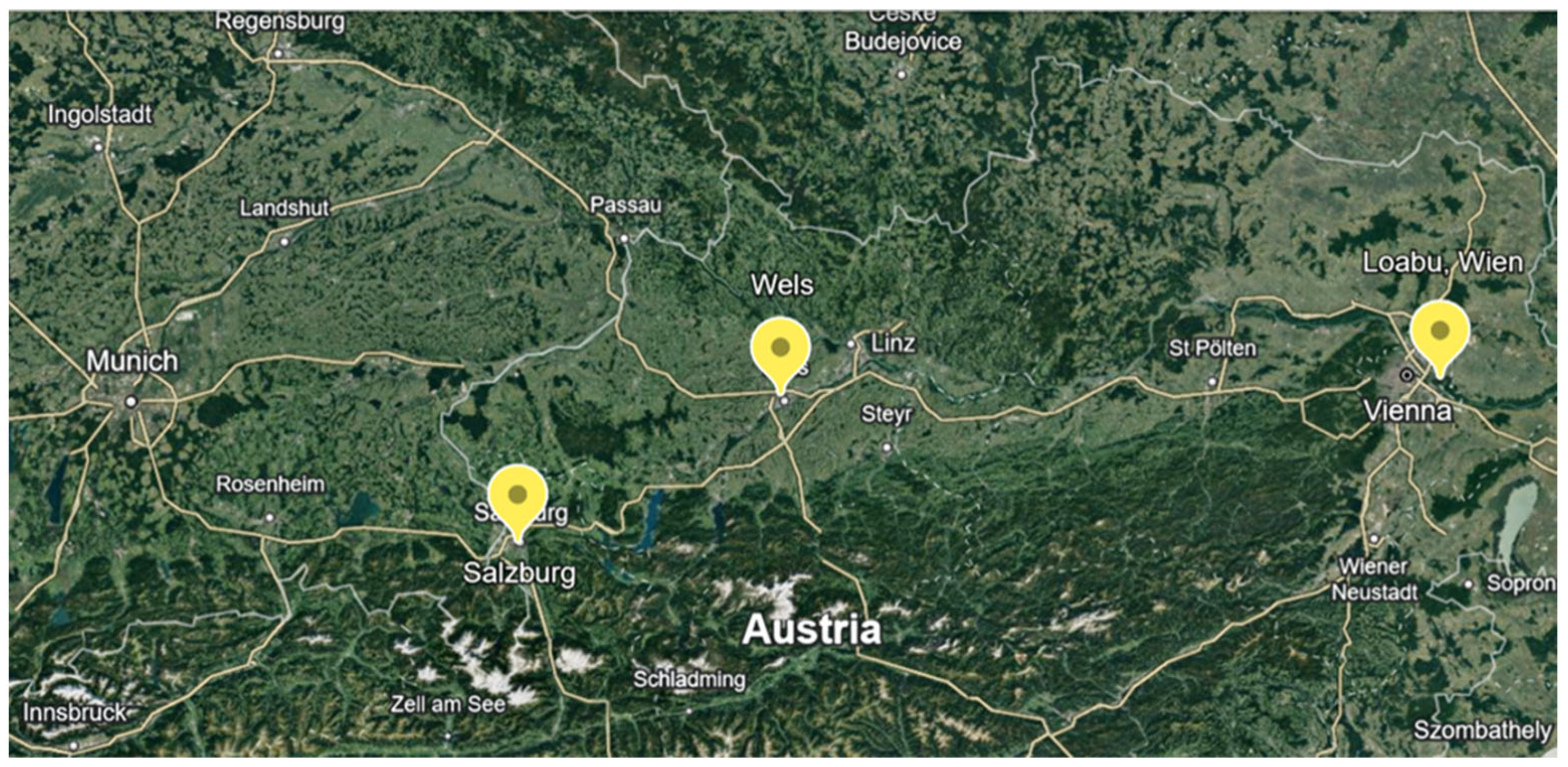
The ground measurement data employed in this analysis are obtained from three stations located in Austria, having high cloud variability that is typical for central Europe. The geographic locations of the stations are depicted in
Figure 1, and period for which data are evaluated is illustrated in
Table 1.
The ground measurement of GHI in this analysis is taken from the Kipp and Zonen CMP11 at Wels and SMP10 pyranometer at Wien with 3% accuracy for daily sum of GHI. The standard benchmark protocol in global GHI forecasting is applied to remove night data, anomalous readings from the pyranometer at dawn and dusk by filtering data based on the solar zenith angle for < 80°. Further, the data for any particular day where there was either shadowing effect or pyranometer calibration problems were removed. The ground measurements data for Wels and Wien are recorded at every 1 min whereas at Salzburg at every 10 min. These data are assembled into hourly average for final result analysis.
2.2. Satellite Data
The satellite data utilized in this research was sourced from the Meteosat satellite, under the operational purview of the European Space Agency (ESA). Positioned at 0 degrees longitude, approximately 36,000 kilometers above the equator, the Meteosat Second Generation (MSG 2), is equipped with the SEVIRI (Spinning Enhanced Visible and Infrared Imager). SEVIRI scans the Earth across 12 distinct spectral channels.
Channel 1 is dedicated to visible light at 0.6 µm, while channel 2 captures visible light at 0.8 µm. Collectively, these are frequently referred to as the "solar channels." Channel 12 is acknowledged as the high-resolution visible channel (HRV) which delivers data with a finer resolution than other solar channels. The HRV channel has a resolution of 1x1 km, whereas the visible 0.6 µm channel offers a resolution of 3x3 km. Readers may refer to the following links for comprehensive details on Meteosat and its diverse array of products [
20,
21,
22].
In this research data from the MSG 0-degree product is used, which features a data update frequency of 15 minutes. Data from channel 1, corresponding to visible light at 0.6 µm is used. The focus is on a small area for each location defined in decimal degree as the aim of the study is apply neural networks to forecast from the extracted data. The areas for the three locations are as follows : Wels : [48.20 - 48,.0 14.0 - 14.2], Wien : [48.30 - 48.10, 16.40 - 16.60] and Salzburg : [47.89 - 47.69, 13.0 -13.20] with the aim of station at the center of respective area.
2.3. Numerical Weather Prediction (GFS) Data
This study utilizes GFS data, accessible for retrieval from the National Centers for Environmental Prediction (NCEP) archive. The data has a temporal resolution of 3 hours and a spatial resolution of 0.250 × 0.250 degrees [
23]. The data interpolation to desired resolution is achieved using method prescribed for the conservation of the solar energy [
24]. In this works, GFS data were provided by Blue Sky Wetteranalysen for Wels and Salzburg [
25] and by Solar Radiation Data (SODA), Mines ParisTech from their archives.
3. Satellite Data to GHI Transformation
3.1. Cloud Index
In this study, the Meteosat MSG 0-degree 1.5B level product data from EUMETSAT is used. The data are downloaded in geotiff format for the specified period for three respective stations mentioned in
Table 1. The detailed study of the components of radiative energy observed by a satellite sensor in a specific spectral band during daytime conditions and the relationships between these components is presented in article [
26]. The downloaded satellite datasets from the Meteosat are already in radiance pixel form following radiometric calibration. The utilization of the geotiff format offers notable advantages, as it can be efficiently processed using the Rasterio library in Python. Moreover, geotiff files exhibit a more compact size in comparison to hdf5 and NetCDF formats. After acquisition, the radiance pixel data is further processed by converting it into a number array format (N1) by using the Rioxarray library.
The pixel array data is then normalized by the cosine of the solar zenith angle to account for first order solar geometry effect [
27].
Clouds have a notably high albedo, signifying their ability to reflect a substantial portion of incident sunlight. Consequently, when observed from above, satellites register a high reflectance ( value in the presence of clouds.
In contrast, the Earth's surface tends to be less reflective, resulting in lower radiance recorded by satellites under clear sky conditions. Notably, a distinctive scenario arises when the ground is blanketed by snow, as snow exhibits a remarkably high reflectivity that can be mistaken for cloud cover. A valuable approach involves leveraging the brightness temperature difference derived from infrared channels to mitigate this under snow conditions [
26].
The Heliosat 2 method is applied for cloud index generation [
28]. To compute the cloud albedo or reflectance (
) and ground reflectance (
), a filtering process is applied, considering only those instances when the sun's elevation angle exceeds 25 degrees. This selective approach is essential due to the sun's position near the horizon during dawn and dusk, leading to very low radiance values. The inclusion of such data can potentially compromise the accuracy of the calculated
and
values [
28].
The cloud index (
) for the observed reflection
for each pixel and time is calculated using the following formula :
Selection of
and
of is a critical task and highly sensitive to atmospheric background profile. Studies have reported using 5
th percentile value for
and 95
th percentile for
from the distribution of
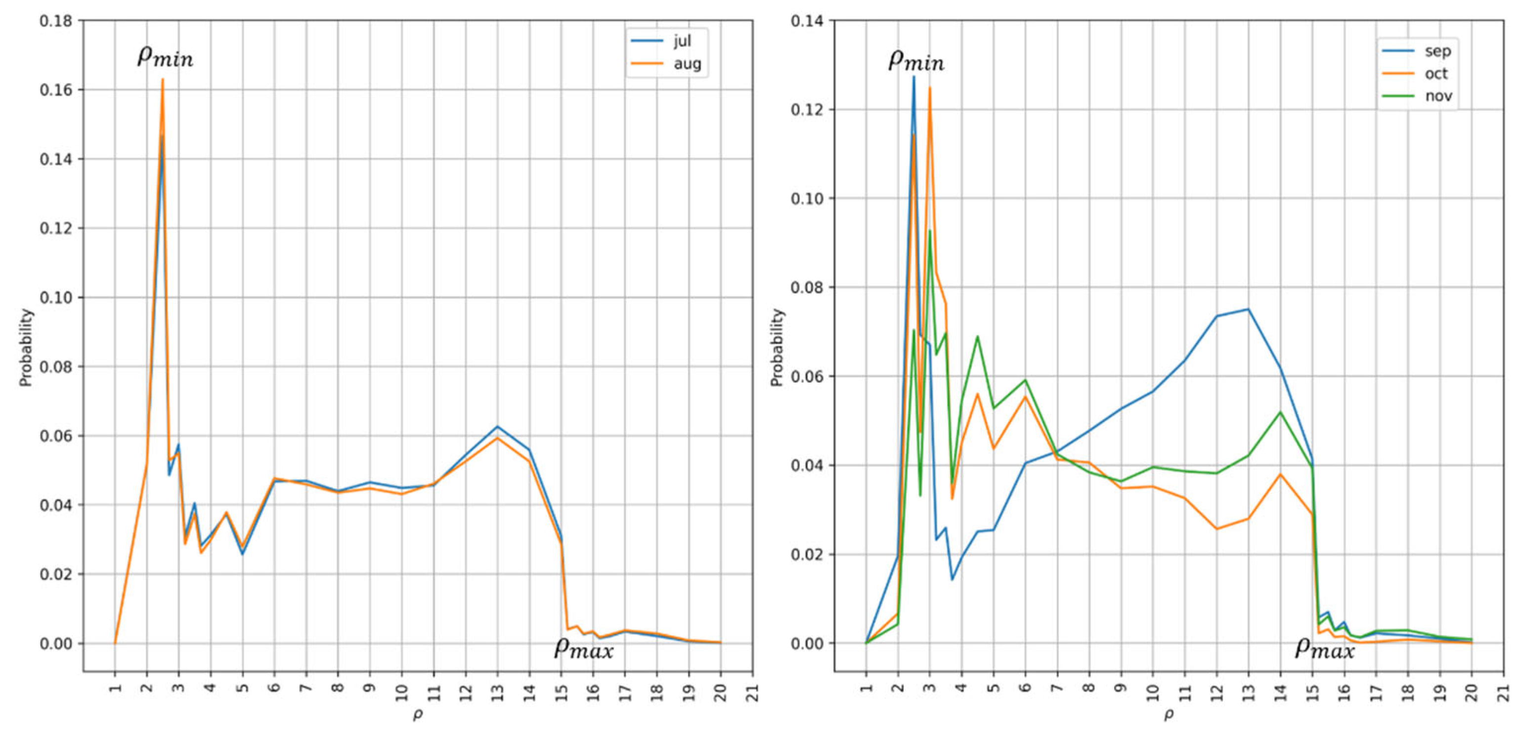
. We experimented with different percentiles and observed that these values are strongly seasonal dependent as well from the probability distribution as shown in
Figure 2 for summer months July and August in comparison to fall months September-November. In this study, 25
th and 99
th percentile for
and
respectively gave consistently best results for all the three stations.
3.2. Clear Sky Index
There exists a direct correlation between the clear sky index and the cloud index in the Heliosat method. The clear sky index is delineated as the quotient of global horizontal irradiance to the irradiance predicted in situations of clear sky conditions.
We modified the equations for the calculation of clear sky index
from the cloud index
as [
30] by introducing an additional second condition
in place of
as follows :
The modified equation yielded statistically improved results especially under the clear sky conditions. The global horizontal irradiance is calculated from the cloud index and by using equations (3) and (4).
3.2. Clear Sky Model Selection
Numerous clear sky models have been introduced in the scientific literature to calculate the solar radiation reaching the Earth's surface under clear sky conditions. These models primarily rely on the position of the sun, input climatic parameters and aerosol content profiles. In this study two widely used models are analyzed and compared.
The
Perez Ineichen clear sky model is renowned for its precision in predicting solar radiation on a horizontal surface coupled with its ease to apply using the open source PVLIB library [
31]. This model offers a reliable method for estimating both the direct and diffuse components of solar radiation in clear sky scenarios. The model typically considers various atmospheric and geographic parameters to estimate the solar radiation, including solar zenith angle, extraterrestrial radiation i.e., the incoming solar radiation at the outer atmosphere, which depends on the Earth-Sun distance and solar declination, optical air mass, turbidity as a measure of the atmospheric clarity, with lower turbidity indicating clearer skies and ground reflectance.
The
McClear sky model was created within the framework of the MACC (Monitoring Atmospheric Composition and Climate) project. This initiative aims to monitor atmospheric composition and assess its influence on climate [
32]. The model considers several input parameters, including the location (latitude and longitude), date, time, and solar zenith angle. It can also utilize atmospheric data from sources like reanalysis datasets. One of the key features of the McClear model is its ability to incorporate information about atmospheric aerosols and water vapor content. This feature enhances its precision in scenarios where these atmospheric factors have a notable impact on solar radiation. The model provides estimates of global horizontal and direct normal solar radiation components under clear sky conditions.
The comparative results of the two models analyzed are discussed in the results
Section 6.1.
4. Performance Metrics
The two predominant metrics employed to assess the accuracy of point forecasts include the mean absolute error (MAE) and the root mean square error (RMSE). In this paper, the aim is to minimize RMSE as lower RMSE is better suited to applications such as grid operation and stability, where high errors are critical [
33], whereas MAE is more suited to applications such as day-ahead markets, which have linear costs relative to error [
34].
where
N represents the number of forecasts, and
represents the actual ground measurement value, and
denotes the forecast value.
The coefficient of determination denoted as R2 or R2 score is a statistical measure commonly used to assess the goodness of fit between observed and predicted values. A higher value for R2 score indicates a more favorable model fit.
The normalized MAE (nMAE) and RMSE (nRMSE) are computed by dividing the respective metrices by the mean value of the measured GHI () for the evaluated test period.
The skill score serves as a critical parameter for assessing model performance when compared to a reference baseline model, typically the smart persistence model in the context of solar forecasting. The skill score (
) of a particular model for the forecast is defined by the following equation :
5. Experimental Setup
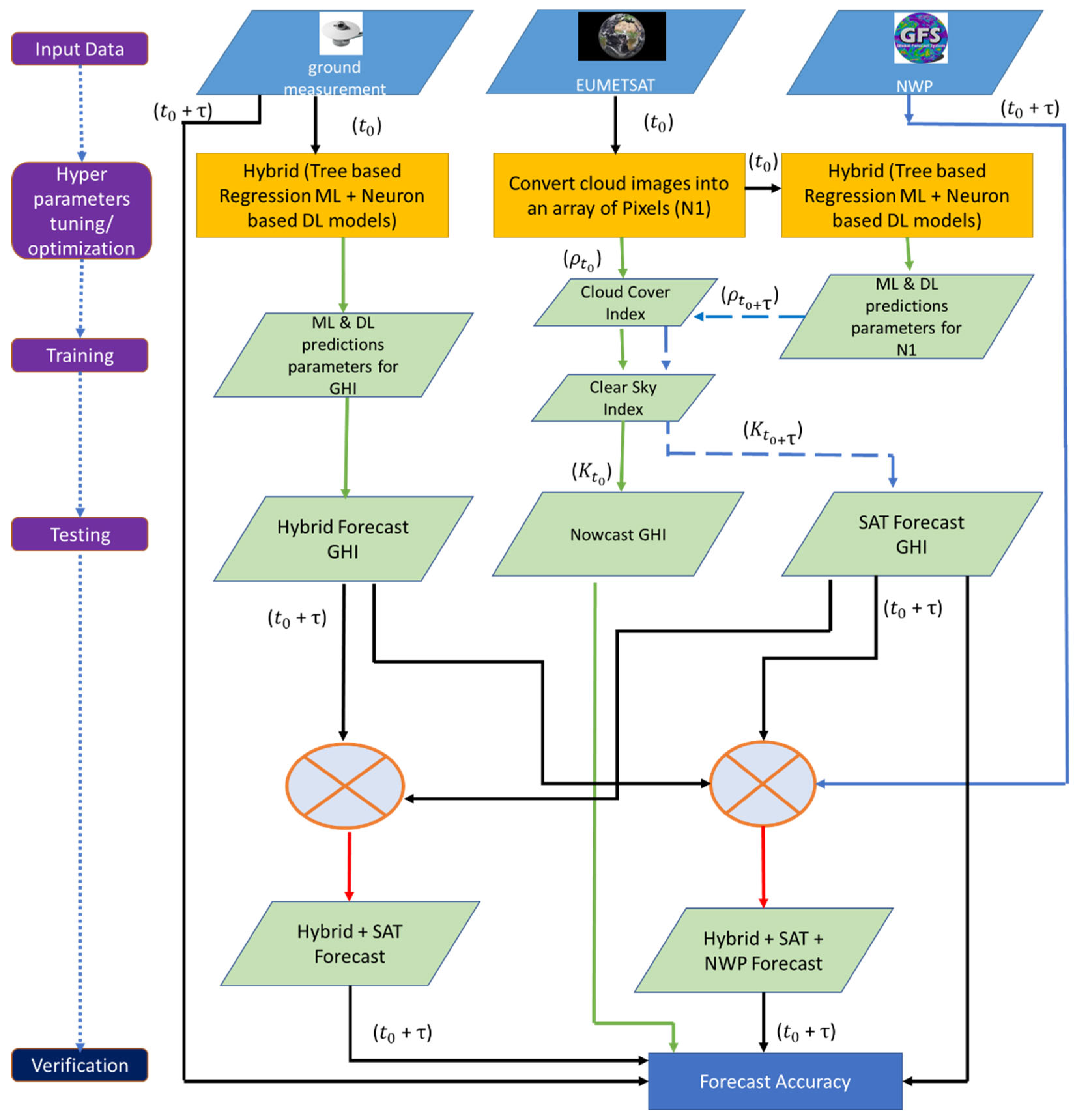
In this study, ML and DL models were analyzed and subsequently hybrid model was developed to allow for higher degrees of model complexity. The methodology employed in this study and the fundamental stages of the modeling and evaluation algorithm for assessing GHI forecasts are depicted in
Figure 3 .
The initial forecast for hourly solar irradiance within the day usually takes place early in the morning, typically between 5:00 and 7:00 local time. This forecast provides predictions for solar irradiance levels throughout the day, broken down into hourly intervals. The exact timing of the first forecast can vary depending on the weather forecasting service or organization providing the information. In view of this, the models are analyzed by issuing the first forecast at 6:00 hr only during daylight hours i.e. when the solar zenith angle
< 80° for the following horizons:
| to |
τ |
∆ |
| Every hour starting at 6:00 hr |
1,2,…6 hr |
15 min |
where to is the forecasting issuing time, τ is forecasting horizon and represents data ∆ aggregation.
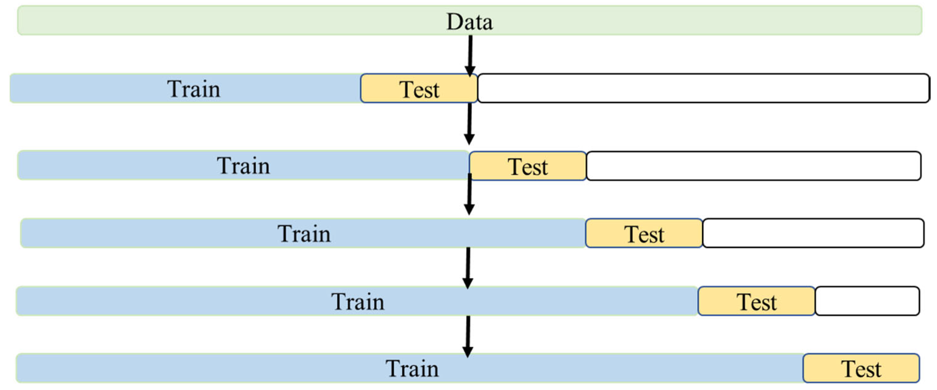
This study utilizes a walk-forward approach, as visualized in
Figure 4, to improve and evaluate the performance of the model. These models are trained for the first three months of the available data and subsequently, trained till the previous month and tested for the following month. The outcomes have shown that this approach can be effectively employed even in situations where a substantial volume of historical data is lacking.
5.1. Models Description
Different models used in this study are listed in
Table 2.
A comprehensive overview of theory and description of ML models which are used for modelling in this study, is presented by authors [
35].
5.1. Deep Learning (DL) Models
5.1.1. LSTM:
LSTM, an abbreviation for Long Short-Term Memory, represents a variation of the Recurrent Neural Network (RNN) concept. The primary objective of this model approach is to effectively capture and retain long-term temporal relationships, mitigating the challenge of vanishing gradients often encountered in conventional RNN [
36]. In addition, LSTM exhibits a noteworthy capability for learning and managing nonlinearity.
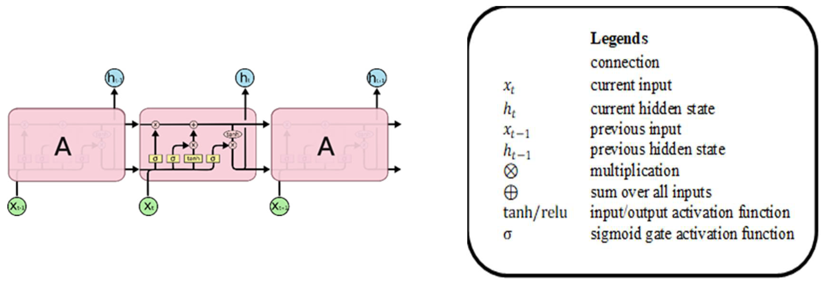
Within the LSTM architecture, memory blocks are constructed, forming an interconnected network designed to sustain and manage information flow over time using nonlinear gating mechanisms.
Figure 5 illustrates the fundamental structure of an LSTM memory cell, encompassing these gating elements, input signals, activation functions, and the resulting output [
37]. Notably, the output of this block is recurrently linked back to the input of the same block, involving all the gate components in this cyclical process.
The step-by-step description of the gates and the mathematical equations associated with them are discussed below:
Forget gate: This step concentrates on updating the forget input component, which entails combining the current input
with the output of that LSTM unit
from the previous iteration, as expressed by the following equation [
37]:
where
are the weight associated with
and
, and
represents standard bias weight vector.
Input gate: In this step a sigmoid layer called input gate decides which value to be updated by combining that combines the current input
, the output of that LSTM unit
[
37].
Cell: A tanh layer creates a vector of new candidate values,
that could be added to the state [
37].
The tanh function squashes input values to the range of −1 to 1 and is symmetric around the origin, with an "S" shape.
In this study, the rectified linear unit (ReLU) activation function is implemented for all deep learning models instead of
, as it has demonstrated superior results during the fine-tuning of hyperparameters. ReLU function is defined as follows:
In other words, for any input x, if x is positive, ReLU returns x, and if x is negative, ReLU returns 0. This results in a piecewise-linear, non-decreasing activation function. Further ReLU has distinct advantages of simplicity and computational efficiency, and it mitigates the vanishing gradient problem in deep networks. This also promotes sparse activation, which can lead to better feature learning.
The fraction of the old state is discarded by multiplying with
and the result is added to the product of current state product
to update the new state [
37]:
Output gate: This step calculates the output gate or the current hidden state and can be depicted as below 37:
Following variants of LSTM model based on the topologies of the layers [
38] are applied in this research :
Vanilla LSTM is the most basic model that has a single hidden layer of LSTM units, and an output layer to make a prediction.
Stacked LSMT: As the name implies, this variation comprises several hidden layers that are arranged one above the other. An LSTM layer by default requires input data in 3D format and will output 2D data.
Bidirectional LSTM: The key feature of this architecture is that it processes input sequences in both forward and backward directions, allowing it to capture information from past and future contexts simultaneously., both of which are connected to the same output layer to combine the interpretations. Bidirectional LSTM achieves a full error gradient calculation by eliminating the one-step truncation that was initially present in LSTM [
38]. Bidirectional processing empowers the model to capture dependencies in both forward and backward directions, proving especially beneficial for tasks where context from future data is significant. Moreover, this model exhibits the ability to capture extended dependencies, thereby enhancing the model's comprehension of the input sequence.
Dense LSTM: The model's inception involves an input layer designed to receive sequential data. There are one or more LSTM layers following the input layer, tailored for the processing of sequential data, as they retain hidden states and capture temporal dependencies. Densely connected layers, often referred to as fully connected layers, are established subsequent to the LSTM layers. These densely connected layers are used to perform various non-linear transformations and reduce the dimensionality of the data.
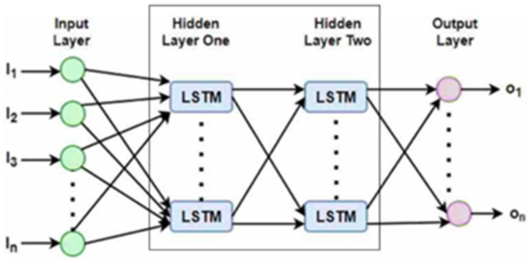
Figure 6 illustrates the typical schematic of sequential flow of a LSTM neural network with all layers, input, and output nodes. The hidden layer nodes are the LSTM cells while dealing with the sequential data.
5.1.2. GRU:
The Gated Recurrent Unit (GRU) is a type of recurrent neural network (RNN) architecture, specifically designed to address some of the limitations of traditional RNNs like vanishing gradients. GRU is a simpler and computationally more economical option compared to the Long Short-Term Memory (LSTM) network, yet it retains the capacity to capture extended dependencies in sequential data.
GRU consists of a solitary hidden layer and two principal gates labeled as the reset gate
and the update gate
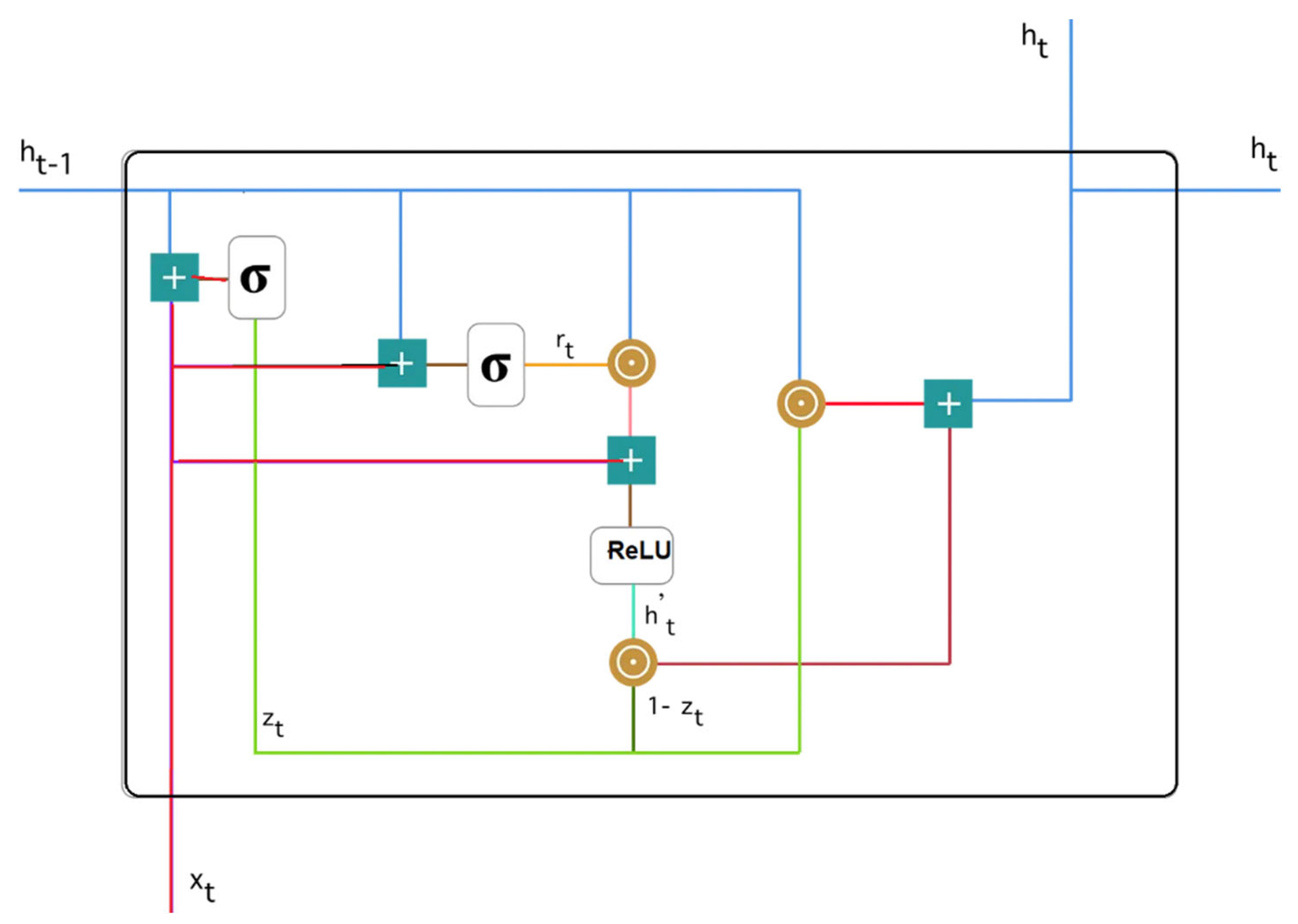
These gates control the flow of information through the hidden state, allowing the network to determine what information to retain and what to discard. Schematic of a typical GRU block is illustrated in
Figure 7 with subsequent equation and functions of each gates [
39].
Update Gate (
) for time step t is derived by using the equation:
where, σ denotes the sigmoid activation function.
denotes weight matrix for the update gate.
is concatenation of the previous hidden state and the current input.
represents the bias term for the update gate.
Reset Gate (
) is akin to the update gate, but it determines what information from the previous hidden state should be erased.
Candidate Hidden State (
): A novel memory component that utilizes the reset gate to retain pertinent information from previous time steps. It is calculated as follows:
where, ⊙ represents element-wise multiplication.
Final Hidden State (
): In the final stage, the network is responsible for computing
, a vector that encapsulates information pertaining to the current unit and transfers it further within the network. To achieve this, the update gate plays a crucial role by discerning what information to gather from the present memory content (
) and what to retain from prior time steps, represented by
.
The advantages of GRU compared to LSTM are threefold: (1) Compared to LSTM, GRU features a more streamlined architecture with a reduced number of gates and less intricate computations. This characteristic simplifies the training and implementation processes. (2) Due to its simplicity, GRU is computationally more efficient than LSTM, which can lead to faster training and inference times. (3) GRU is a good choice for tasks where capturing short-term dependencies in sequences is sufficient, and a more complex model like LSTM may not be necessary. However, GRU has limited capacity in capturing very long-term dependencies in sequences, as it doesn't have a dedicated cell state like LSTM. LSTM is better suited for tasks that require modeling long-range dependencies.
5.1.2. DL Voting Ensemble model:
A voting ensemble model from optimized stacked LSTM, Bidirectional LSTM, Dense and GRU is built. This is achieved by loading the pretrained models and making predictions by individual models known as base models. Input layers are defined for the ensemble model. These input layers are used to feed the predictions of the individual models into the ensemble.
The output tensors of the individual models are obtained by passing the input layers as inputs to each model. This produces output1, output2, output3, and output4, which represent the outputs of each LSTM model. An ensemble layer is then created using the average() function, which averages the outputs of the individual models (output1, output2, output3, and output4). Averaging is a common method for combining predictions in a Voting Ensemble for LSTM based models.
The ensemble model is then defined using the model class from Keras. The input layers and the ensemble layer are specified as inputs and outputs, respectively. This creates a new model called Ensemble model that takes predictions from the four models and produces an ensemble prediction. The ensemble model is compiled with the Adam optimizer and the mean squared error (MSE) loss function. Additionally, accuracy is tracked as a metric.
Leveraging a Voting Ensemble with diverse LSTM models is a potent strategy for enhancing the precision and resilience of predictions. It utilizes the diversity of multiple LSTM models to provide more reliable results, making it a valuable tool in various machine learning and sequence modeling tasks.
Recent literature demonstrates an increasing research interest in the utilization of deep learning models for predicting solar irradiance for intra-day and intra-hour forecast horizons [
40,
41,
42,
43,
44,
45].
5.2. Weighted Average Ensmble Model
In an ensemble model, particularly an average ensemble, the combined forecast obtained by averaging the predictions of each individual model is evaluated for each hour of the day, as expressed by the Equation 19:
With the primary aim of minimizing RMSE in short-term intra-day forecasting, the weighted average ensemble approach computes the performance weight of each model for different hours of the day by employing the reciprocal of RMSE. For instance, the weight assigned to the forecast of model
is determined as follows:
where
i.e., inverse of RMSE for respective models.
The forecast generated by the weighted average ensemble is subsequently assessed on an hourly basis by Equation 21.
The hybrid model is intricately designed to begin by independently computing the hourly weights for each individual ML and DL model. Following this calculation, rankings are assigned based on the cumulative weight of each model, and the six top-performing models are automatically selected according to their ranking in a weighted average ensemble model. This methodology empowers the selection of the most effective models, while simultaneously optimizing the trade-off between bias and variance. The selected model is labeled as Hybrid (Hyb) model in the subsequent analaysis and discussion.
Additionally, we assess cases where a hybrid model is combined with satellite data referred to as (Hyb + SAT), as well as scenarios where it is further enhanced by integrating GFS forecast data, labeled as (Hyb + SAT + NWP).
5.3. Baseline Naive Model
In academic literature, a typical approach involves comparing the outcomes of the proposed models with those of simpler or reference models to evaluate the enhancements. A commonly employed reference model is the Smart Persistence model [
46]. The Smart Persistence model exclusively relies on historical ground radiation data from the specific location and utilizes clear sky index series. It forecasts the clear sky index for each time horizon τ as the average of the τ preceding clear sky values [
47]. In statistical terms it is also defined as rolling mean and is defined by the equation:
Similar methodology is applied for N1 pixel to calculate the persistence value of N1.
5.3. Joint and Marginal Distribution
The distribution-based forecast verification framework offers a robust method for evaluating a model's performance by analyzing the extent to which the forecasted values diverge from the observed value ranges [
48].
The interconnection among joint, marginal, and conditional distributions of two random variables can be statistically expressed through the application of Bayes' theorem. In the specific context of meteorology, where these variables pertain to forecast and observation, this very association is recognized as the Murphy-Winkler factorization expressed as [
49] :
where,
is the probability of both events,
and
, occurring simultaneously.
denotes the conditional probability of event occurring given that the event f has already occurred.
denotes the probability of event occurring.
denotes the conditional probability of event occurring given that the event has already occurred.
represents the probability of event occurring.
The joint probability of both events happening, referred to as , is computed as the product of the conditional probability of given and the probability of .
5.4. Feature Engineering
Feature engineering serves as a pivotal step in both machine and deep learning pipelines, enabling the transformation of raw data into a more informative and suitable format for training and enhancing model performance. Its significance extends to influencing the bias-variance trade-off, thereby mitigating overfitting and underfitting in machine learning models. The bias-variance trade-off aims to find a balance between underfitting and overfitting. Feature engineering is a key tool for achieving this balance because it allows to control the model's complexity by techniques like dimensionality and noise reduction, regularization, feature expansion.
In the context of satellite pixel data, which has a sampling frequency of 15 minutes, we employ the Fourier transform on both the hourly and quarter-hourly (15 minutes, denoted as 'minute') values. This transformation allows us to identify and extract the predominant frequency components that encapsulate the most significant recurring patterns within the dataset. Subsequently, these frequency components are harnessed as crucial input features for ML and DL models. The value of is in range of 1-5 for and while extracting fourier transform of hour and quarter hour.
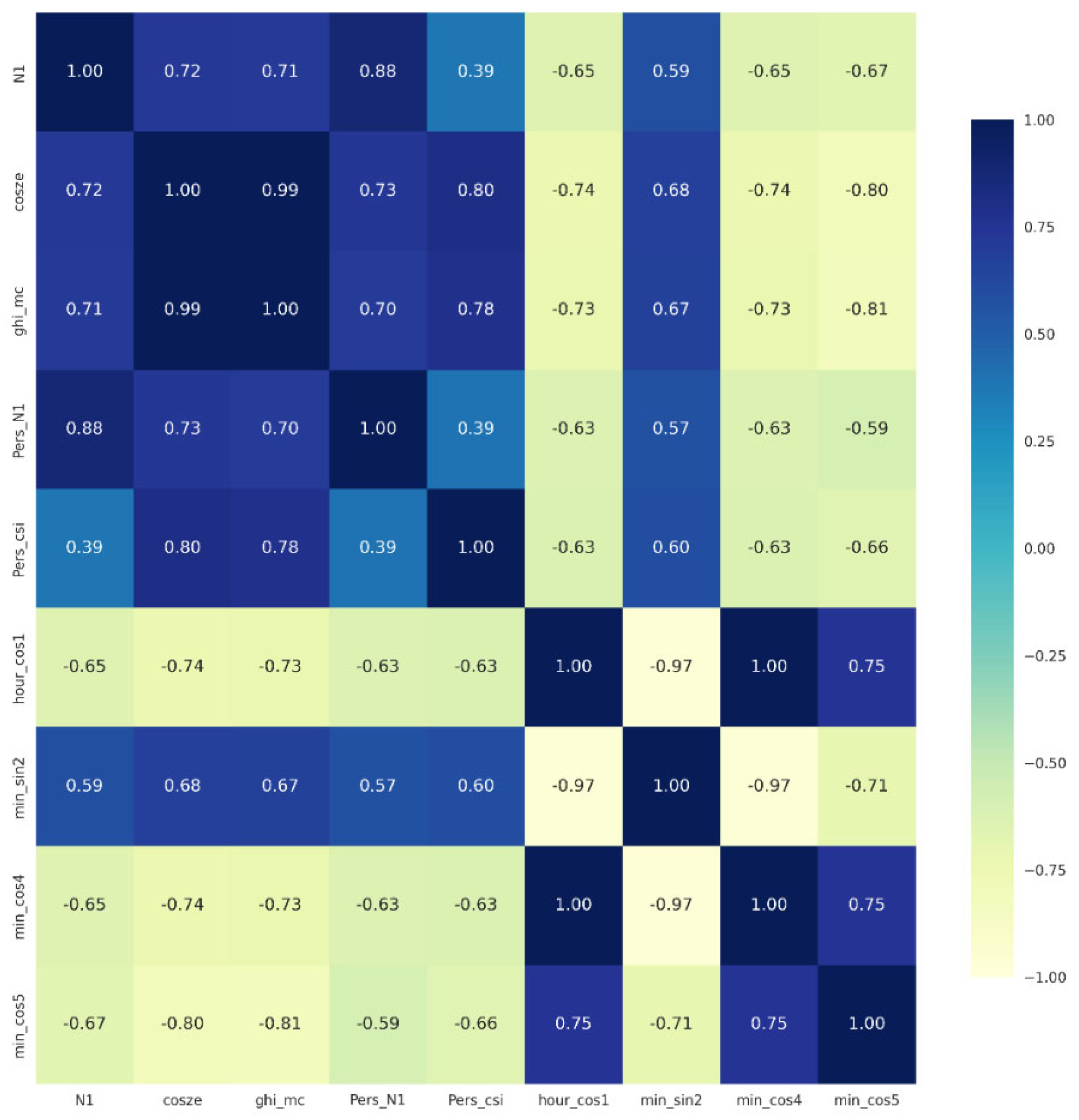
Important features are extracted by applying feature importance assessment using Random Forest and XGB by randomly selecting 10 days of data for each month. These features are further examined using correlation method. Specifically, features exhibiting a correlation value greater than |0.3| with N1 are deemed pertinent as illustrated in heatmap
Figure 8 for Wien station and subsequently used for the modeling, where :
N1 : Satellite Pixel value (target)
cosze : ghi_mc : McClear GHI value (scaled using min-max scaler)
Pers_N1 : Persistent N1 value as defined by Equation 22
Pers_csi : Persistent clear sky index, ( as defined by Equation 22
hour_cos1 : Fourier transform cosine of hour with k = 1
min_sin2 : Fourier transform sin of quarter hour with k = 2
min_cos4 : Fourier transform cosine of quarter hour with k = 4
min_cos5 : Fourier transform cosine of quarter hour with k = 5
The feature importance for other stations also exhibit similar patterns.
Figure 8.
Heatmap showing correlation of N1 with features used in modelling.
Figure 8.
Heatmap showing correlation of N1 with features used in modelling.
6. Results and Discussion
6.1. Overview and Analysis Clear Sky models
The following observations emphasize the importance of understanding and accounting for the deviations of satellite derived GHI from measurements when applying clear sky models for GHI estimation.
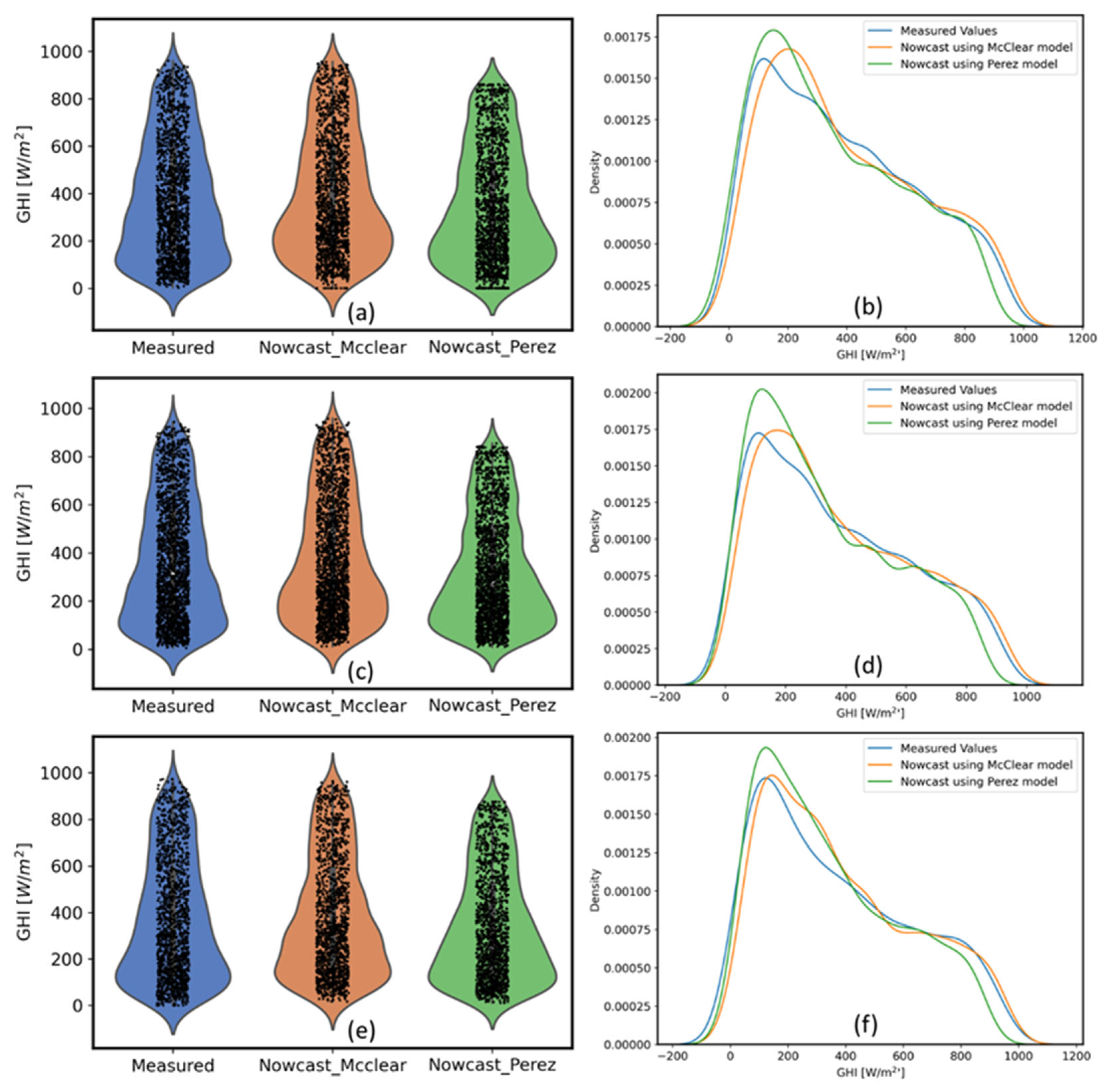
GHI is calculated from the Satellite derived clear sky index using Equation 3 by applying two clear sky models. The violin and distribution plots in
Figure 9 clearly show that Perzel clear sky model deviates from ground measurements significantly under the clear sky conditions with GHI above 800 W/m
2. Both the models show statistically significant deviation from ground measurement data around 150-180 W/m
2. But Perez model shows sharp deviation from ground measurements between 200-400 W/m
2.
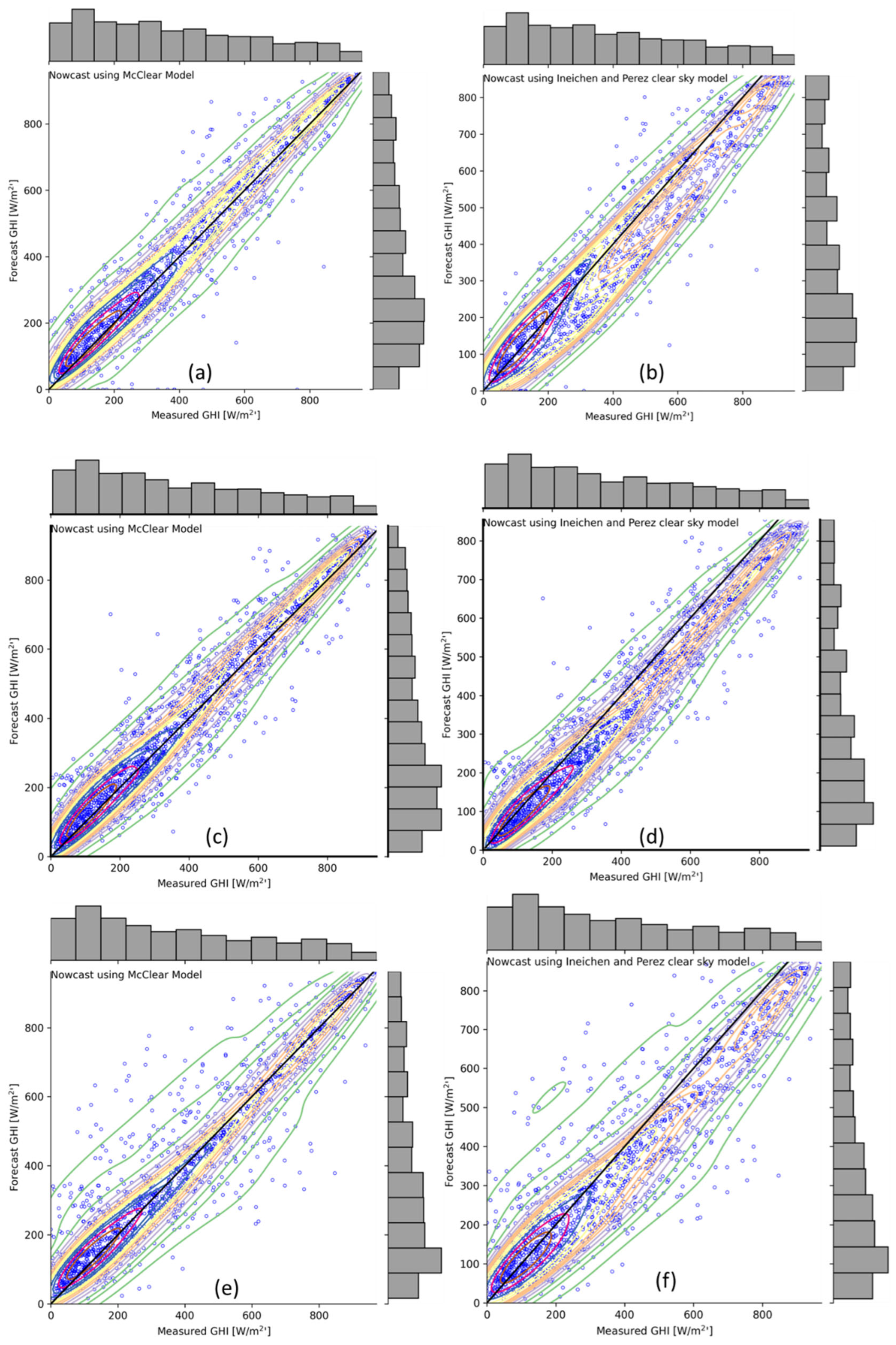
In this study, the joint and marginal distributions of the nowcast Global Horizontal Irradiance (GHI) obtained from the McClear and Perez models, comparing to ground observations collected at three monitoring stations is analyzed.
Figure 10 depicts the visual representation of these distributions where the diagonal black line corresponds to the ground measurements.
For the joint distribution using the McClear model, roughly equal probabilities are observed on both sides of the diagonal. However, GHI calculated using the Perez model, it is discovered that it tends to underpredict GHI. This is evident as the probability density is higher below the diagonal line, confirming that the Perez model's predictions () are less than the observed values ().
A significant pattern is observed upon closer inspection of the 2D kernel density contours. For low-irradiance conditions, the satellite-derived GHI using the McClear model exhibits a slight upward drift above the diagonal line. Conversely, the Perez model shows the opposite behavior, with the GHI prediction drifting below the diagonal.
We also note a distinct characteristic regarding the satellite observations at the Salzburg location. These observations exhibit greater dispersion compared to the other two monitoring sites. This disparity might be ascribed to the frequency of data collection in Salzburg, which occurs at 10-minute intervals. This interval could potentially introduce an aggregation effect in the ground measurement errors when these data points are averaged to an hourly resolution. In contrast, the other two sites provide ground measurement data at a 1-minute resolution, potentially resulting in fewer aggregation-induced discrepancies.
These observations offer valuable insights into how the McClear and Perez models perform comparing with ground-based GHI measurements particulary in central europe. They affirm that the McClear model surpasses the Perez model in terms of performance. This is further substantiated by the error metrics in
Table 3 for the two models for the GHI derived using satellite data. In light of these observations, McClear model is applied for further work and assessment of forecast models.
6.2. Satellite Derived GHI
The quality of GHI data obtained from METOSAT satellite pixels is demonstrated through a time series plot dated June 24, 2021 for Wels, presented in
Figure 11. This figure highlights three specific scenarios: (a) clear sky conditions, (b) cloudy conditions, and (c) partially cloudy conditions. These specific events are graphically compared by images (d, e, f) acquired by an All Sky Imager (ASI) with their corresponding satellite cloud images (m, n, o). Green arrows in the satellite cloud images represent cloud motion vectors, indicating cloud movement and direction. The cloud mask and pixel images from EUMETSAT are depicted in (g, h, i) and (j, k, l), respectively.
The station's position is marked at the center of the red square box in the satellite cloud and cloud mask images. Within the cloud mask images (g, h, i), the presence of green indicates clear sky regions, whereas the white areas correspond to cloud coverage. In the RGB images (j, k, l), the green areas signify clear skies, the light yellow regions represent scattered clouds, and the dark blue and black regions denote the presence of heavily overcast dark clouds. These images, corresponding to the three identified events in the time series plot, clearly demonstrate a correlation and the effectiveness of our algorithm in accurately capturing clear sky, cloudy, and partially cloudy conditions.
6.3. Hybrid Model Result Analysis
Table 4 presents a summary of RMSE (W/m
2) values for various individual models utilized in this study, as well as ensemble models and the ultimate hybrid model constructed using six top-performing models. The hybrid model is denoted in bold font, while the voting ensemble model derived from deep learning (DL) models is highlighted in italics, and the voting ensemble model based on machine learning (ML) models is emphasized in bold italics. The table also showcases the percentage improvement (%) of the hybrid model over the least performing individual model, as well as the corresponding improvement for the voting ensemble models compared to its lowest-performing constituent model for ML and DL respectively.
The hybrid model exhibits a remarkable improvement, enhancing the RMSE score by 4.1% to 10.6% across various forecast horizons. These results also reveal that voting is a superior choice compared to stacking when it comes to ML ensemble models. Moreover, the performance of the ML voting ensemble model exhibits enhancement as the forecast horizon extends, whereas the opposite trend is observed for the DL voting ensemble model.
Comparable findings are observed at the other two locations, clearly underscoring the benefits of employing a hybrid model as opposed to relying on a single model for forecasting purposes.
Table 4.
RMSE of different models for Wien station for different forecast horizons.
Table 4.
RMSE of different models for Wien station for different forecast horizons.
| Model |
1h |
2h |
3h |
4h |
5h |
6h |
| Hybrid Model |
101.181 (7.54%) |
124.834 (4.19%) |
136.622 (10.61%) |
142.699 (4.73%) |
144.507 (6.34%) |
140.393 (5.95%) |
| DL Voting |
101.221 (7.5%) |
125.664 (3,56%) |
139.943 (10.26%) |
145.247 (4.7%) |
145.774 (4%) |
141.543 (2.66%) |
| ML Voting |
101.276 (4.22%) |
124.634 (3.98%) |
136.669 (3.83%) |
143.928 (5.33%) |
145.38 (5.78%) |
140.946 (5.81%) |
| Bi-Directional |
101.418 |
130.301 |
142.967 |
144.964 |
151.574 |
143.528 |
| XGBoost |
103.026 |
127.150 |
137.152 |
144.763 |
145.513 |
141.565 |
| Gradient Boost |
103.314 |
126.081 |
139.604 |
146.818 |
147.827 |
140.809 |
| SVM |
103.380 |
129.801 |
143.486 |
152.027 |
154.298 |
149.281 |
| Random Forest |
103.405 |
126.350 |
140.630 |
146.934 |
150.748 |
145.852 |
| Stacking |
104.002 |
127.956 |
141.872 |
151.906 |
151.991 |
145.721 |
| LSTM Stacking |
104.797 |
129.407 |
152.842 |
148.595 |
148.483 |
144.803 |
| kNN |
105.738 |
129.504 |
142.113 |
149.786 |
150.978 |
144.438 |
| Dense |
105.895 |
129.624 |
140.953 |
145.759 |
147.138 |
143.401 |
| GRU |
109.432 |
126.941 |
138.595 |
150.839 |
148.559 |
144.141 |
6.4. Forecast Results
In this segment, we provide an assessment of intra-day GHI forecst upto 6 hr generated by the various models, conducting a comparative analysis to determine the performance of models. Following this, we perform an in-depth examination of forecast performance across different clusters of clear sky indices.
Table 5,
Table 6 and
Table 7 provide an analysis of forecast performance for three distinct stations, measured in terms of RMSE in units of W/m². Each row in these tables represents different forecasting models and combinations of models used in this research. The results emphasise the consistent and superior performance of all the developed models in comparison to the smart persistence model. Notably, during the first hour of the forecast, the GFS exhibits subpar performance, aligning with existing literature that highlights challenges in initializing atmospheric boundary conditions for NWP models.
The combination of the hybrid ensemble model, comprising the hybrid model in conjunction with satellite and NWP models (Hyb+SAT+NWP), surpasses all other models across all forecast horizons. Nonetheless, it is important to acknowledge that the RMSE error tends to rise as the forecast horizon is extended, as anticipated. The percentage increase in RMSE by the smart persistence model over a 1-hour to 6-hour interval falls spanning within the range of {28.84% - 47.54%}, {36.76% – 70.92%}, and {28.78% – 71.93%}, for Wien, Salzburg, and Wels respectively. In contrast, the corresponding rate of increase observed for the hybrid ensemble model (Hyb+SAT+NWP) across the same time frame is in the range of {16.95% - 28.79%}, {20.67% – 44.14%}, and {17.68% – 51.18%} for the respective three stations. The relatively modest rise in RMSE for our models over extended time horizons underscores the efficiency of the model.
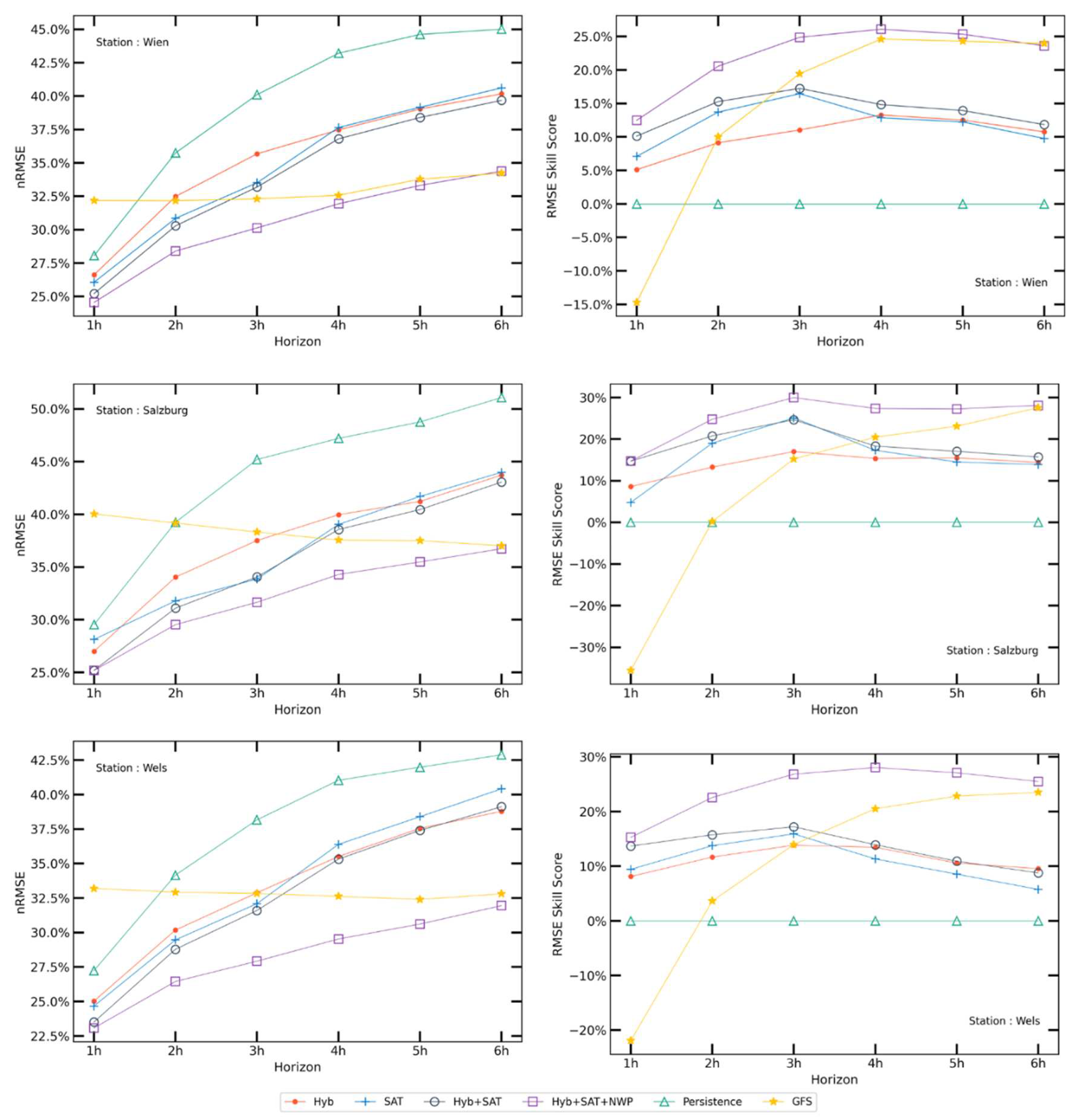
Figure 12 illustrates the normalized nRMSE (%) and RMSE skill score for all models across various time horizons at each station. Notably, SAT results consistently outperform the hybrid model up to a 3-hour horizon, beyond which the hybrid model's performance exhibits marginal improvement over SAT. This observation aligns with the fact that satellite data corresponds to time lags from
to
hr.
The combination of hybrid+SAT presents a distinct advantage over individual models, with the effect becoming more pronounced up to a 3-hour lead time. Beyond this point, the addition of NWP offers a clear advantage for all three locations as the time horizon increases. In terms of performance, Hybrid+SAT+NWP remains nearly unchanged when compared to the combination of Hybrid+SAT during the first hour, but afterward, it delivers a 5% to 20% improvement in skill score from 2 to 6 hours ahead.
In the case of a 6-hour ahead forecast, the best-performing (Hyb+SAT+NWP) model only demonstrates a marginal advantage over the NWP model for Salzburg and Wels, while the situation is reversed for Wien.
The best performing model (Hybrid+SAT+NWP) is further assessed in terms of skill score by categorizing day types according to the daily average clear sky index values, as outlined in
Table 8 and the results are shown in
Figure 12 for all three stations [
35].
This analysis vividly reveals that, for overcast days (DT1), the model's performance lags behind that of the smart persistence model, particularly in the 1-hour ahead forecast. This finding corroborates our earlier observations, as depicted in the 2D kernel density contours in
Figure 10, wherein SAT forecasts exhibit a higher bias for lower values of GHI in cases of overcast conditions. Nevertheless, it is important to highlight that this distinction does not wield a statistically significant impact on the overall results. This is because the total number of overcast days (DT1) amounts to 28, 22, and 20 for Wien, Salzburg, and Wels, respectively, with an average GHI value of approximately 30 W/m
2 for such days. Should the forecast values for the 1-hour ahead prediction be adjusted to match the smart persistence values, the overall RMSE improvement for the entire test period is only around 2-3 W/m
2 for 1h ahead forecast with this correction.
A closer examination of the results by this method highlights the model's competency in capturing extremely high cloud variability during cloudy and heavily clouded sky conditions, resulting in a skill score improvement ranging from 10% to 30%.
7. Conclusion and Future Work
The primary goal of this research was to apply satellite data to enhance the accuracy of intra-day GHI predictions, spanning from 1 to 6 hours into the future, with an hourly time resolution. The study demonstrated the benefits of employing a hybrid model that harnesses the optimal performance of individual models across various temporal horizons, combining both machine learning (ML) and deep learning (DL) models. This study investigated the benefits of combining hybrid model with models based on satellite imagery and numerical weather prediction (NWP) for improving intra-day solar radiation forecasts and proved that Hybrid+SAT+NWP is the optimal choice for short term hourly intra-day solar radition forecasting. The nRMSE and RMSE skill score values demonstrate remarkable performance, exceeding the results commonly found in literature. This achievement is particularly noteworthy, considering the limited dataset, which covers less than a year of measurements and originates from experimental sites in central Europe, where unpredictable cloudy weather conditions are prevalent.
This research yielded several additional noteworthy findings. Firstly, it introduced a consistent and highly accurate method of deriving GHI based on satellite imagery. Secondly, this study emphasized the significance of using an appropriate clear sky model when deriving GHI from satellite-based sources. A comprehensive comparative analysis of the Perez and McClear models clearly highlighted the advantages of the McClear model. The study also highlighted the importance of classifying different day types based on clear sky indices and underscored the benefits of the blending model, particularly on cloudy and highly cloudy days.
In light of the findings of this study, there are serveral valuable avenues for future research. First, in order to enhance forecasting accuracy, we recommend exploring the utilization of the European Centre for Medium-Range Weather Forecasts (ECMWF) as the primary source for NWP input data. Additionally, the incorporation of additional meteorological variables such as temperature, relative humidity, and wind speed as exogenous features needs to be investigated further.
Moreover, a promising area for future research involves conducting a more detailed analysis of historical large-scale satellite data. This analysis would focus on uncovering the precise temporal and seasonal correlations of and , thereby contributing to the refinement and increased accuracy of GHI derivation from satellite-based pixels.
The joint and marginal distribution analysis warrants a condition-based post processing treatment of irradiance to correct satellite based GHI calculations which can possibly enhance the forecasting accuracy to next level.
Author Contributions
Conceptualization, J.T.; formal analysis, J.T.; software, J.T. and M.K; visualization, J.T.; validation, J.T.; writing—original draft preparation, J.T.; writing—review and editing, R.H.; project administration, R.H.; supervision, R.H. All authors have read and agreed to the published version of the manuscript.
Institutional Review Board Statement
Not applicable.
Informed Consent Statement
Not applicable.
Data Availability Statement
Not applicable.
Acknowledgments
We thank Wolfgang Traunmüller of Blue Sky Wetteranalysen for sharing ground measurement data and GFS data for Salzburg and Jean-Baptiste Pellegrino of Solar Radiation Data (SODA) Mines ParisTech for sharing GFS data from their archives for Wien and giving access to McClear clear sky model data for all stations. We also thank Douglas Vaught for reviewing the manuscript.
Conflicts of Interest
The authors declare no conflict of interest.
Abbreviations
| PV |
Photovoltaics |
GHI
EUMETSAT
SEVIRI
MSG
CMV
CMF |
Global Horizontal Irradiance
European Organisation for the Exploitation of Meteorological Satellites
Spinning Enhanced Visible and Infrared Imager
Metosat Second Generation
Cloud Motion Vector
Cloud Motion Field |
| Kt
|
Clear Sky Index |
ML
DL
AI |
Machine Learning
Deep Learning
Artificial Intelligence |
| ANN |
Artificial Neural Network |
| GFS |
Global Forecast System |
| ECMWF |
European Centre for Medium Range Forecasts |
| NWP |
Numerical Weather Prediction |
| RF |
Random Forest |
| GB |
Gradient Boosting |
XGB
kNN
SVM
Stacking
voting
LSTM
biDir
dense
stacked
GRU
DL_voting
R2
SS |
Extreme Gradient Boosting
k-Nearest Neighbors
Support Vector Machine
Stacking Ensemble of ML models
Voting Ensemble of ML models
Long Short-Term Memory
Bi-Directional LSTM
Dense LSTM
Stacked LSTM
Gated Recurrent Unit
Voting Ensemble of DL models
Coefficient of Determination score
Skill Score |
| MBE |
Mean Bias Error |
| MAE |
Mean Absolute Error |
| nMAE |
Normalized Mean Absolute Error |
| RMSE |
Root Mean Square Error |
| IRMSE |
Inverse of RMSE |
| nRMSE |
Normalized Root Mean Square Error |
References
- D. Heinemann, E. Lorenz, M. Girodo, Forecasting of Solar Radiation. Solar Energy Resource Management for Electricity Generation from Local Level to Global Scale, Nova Science Publishers, New York, 2006.
- R. Perez, E. Lorenz, S. Pelland, M. Beauharnois, G. Van Knowe, K. Hemker, D. Heinemann, J. Remund, S. Müller, W. Traunmüller, Comparison of numerical weather prediction solar irradiance forecasts in the US, Canada and Europe, Sol. Energy 94 (2013) 305 326. [CrossRef]
- Thaker, J.; Höller, R. Hybrid Numerical Ensemble Method and Comparative Study for Solar Irradiance Forecasting. In Proceedings of the 8th World Conference on Photovoltaic Energy Conversion, Milan, Italy, 26–30 September 2022; pp. 1276–1284. [CrossRef]
- Verbois, Hadrien; Saint-Drenan, Yves-Marie; Thiery, Alexandre; Blanc, Philippe (2022): Statistical learning for NWP post-processing: A benchmark for solar irradiance forecasting. [CrossRef]
- Maimouna Diagne, Mathieu David, Philippe Lauret, John Boland, Nicolas Schmutz, Review of solar irradiance forecasting methods and a proposition for small-scale insular grids, Renewable and Sustainable Energy Reviews, Volume 27, 2013, Pages 65-76, ISSN 1364-0321. [CrossRef]
- J. Antonanzas, N. Osorio, R. Escobar, R. Urraca, F.J. Martinez-de-Pison, F. Antonanzas-Torres, Review of photovoltaic power forecasting, Solar Energy, Volume 136, 2016, Pages 78-111, ISSN 0038-092X. [CrossRef]
- R. A. Rajagukguk, R. Kamil, and H.-J. Lee, “A Deep Learning Model to Forecast Solar Irradiance Using a Sky Camera,” Applied Sciences, vol. 11, no. 11, p. 5049, May 2021. [CrossRef]
- Edited by Manajit Sengupta, Aron Habte, Christian Gueymard, Stefan Wilbert, Dave Renne, Thomas Stoffel. Best Practices Handbook for the Collection and Use of Solar Resource Data for Solar Energy Applications: Second Edition.
- Perez, R., Cebecauer, T., Šúri, M., 2013. Chapter 2 - semi-empirical satellite models. In: Kleissl, J. (Ed.), Solar Energy Forecasting and Resource Assessment. Academic Press, Boston, pp. 21–48.
- Perez, R., Ineichen, P., Moore, K., Kmiecik, M., Chain, C., George, R., Vignola, F., 2002. A new operational model for satellite-derived irradiances: description and validation. Sol. Energy 73 (5), 307–317. [CrossRef]
- Laguarda, A., Giacosa, G., Alonso-Suárez, R., Abal, G., 2020. Performance of the siteadapted CAMS database and locally adjusted cloud index models for estimating global solar horizontal irradiation over the Pampa Húmeda. Sol. Energy 199, 295–307. [CrossRef]
- Lorenz, E., Hammer, A., Heinemann, D., et al., 2004. Short term forecasting of solar radiation based on satellite data. In: EUROSUN2004 (ISES Europe Solar Congress). pp. 841–848.
- Lucas, B.D., Kanade, T., 1981. An iterative image registration technique with an application to stereo vision. In: Proceedings of the 7th International Joint Conference on Artificial Intelligence - Volume 2. IJCAI’81, Morgan Kaufmann Publishers Inc., San Francisco, CA, USA, pp. 674–679.
- Aicardi D, Musé P, Alonso-Suárez R. A comparison of satellite cloud motion vectors techniques to forecast intra-day hourly solar global horizontal irradiation. Solar Energy. 2022;233:46–60. [CrossRef]
- Aguiar LM, Pereira B, Lauret P, Díaz F, David M. Combining solar irradiance measurements, satellite-derived data and a numerical weather prediction model to improve intra-day solar forecasting. Renewable Energy. 2016;97:599–610. [CrossRef]
- B. Benamrou, M. Ouardouz, I. Allaouzi, and M. Ben Ahmed, “A Proposed Model to Forecast Hourly Global Solar Irradiation Based on Satellite Derived Data, Deep Learning and Machine Learning Approaches,” J. Ecol. Eng., vol. 21, no. 4, pp. 26–38, May 2020. [CrossRef]
- J. H. Jeppesen, R. H. Jacobsen, F. Inceoglu, and T. S. Toftegaard, “A cloud detection algorithm for satellite imagery based on deep learning,” Remote Sensing of Environment, vol. 229, pp. 247–259, Aug. 2019. [CrossRef]
- B. Ameen, H. Balzter, C. Jarvis, and J. Wheeler, “Modelling Hourly Global Horizontal Irradiance from Satellite-Derived Datasets and Climate Variables as New Inputs with Artificial Neural Networks,” Energies, vol. 12, no. 1, p. 148, Jan. 2019. [CrossRef]
- Tajjour S, Chandel SS, Malik H, Alotaibi MA, Márquez FPG, Afthanorhan A. Short-Term Solar Irradiance Forecasting Using Deep Learning Techniques: A Comprehensive case Study. IEEE Access. 2023:1. [CrossRef]
- https://www.eumetsat.int/seviri.
- https://www.eumetsat.int/meteosat-second-generation.
- https://www.eumetsat.int/0-degree-service.
- National Centers for Environmental Prediction/National Weather Service/NOAA/U.S. Department of Commerce. 2015, updated daily. NCEP GFS 0.25 Degree Global Forecast Grids Historical Archive. Research Data Archive at the National Center for Atmospheric Research, Computational and Information Systems Laboratory. [CrossRef]
- Lorenz, Elke, et al. "Comparison of global horizontal irradiance forecasts based on numerical weather prediction models with different spatio-temporal resolutions." Progress in Photovoltaics: Research and Applications 24.12 (2016): 1626-1640. [CrossRef]
- Natschläger, T.; Traunmüller, W.; Reingruber, K.; Exner, H. Lokal optimierte Wetterprognosen zur Regelung stark umweltbeeinflusster Systeme; SCCH, Blue Sky. In Tagungsband Industrielles Symposium Mechatronik Automatisierung; Clusterland Oberösterreich GmbH/Mechatronik-Cluster, Wels: 2008; pp. 281–284.
- Alexander P. Trishchenko, Solar Irradiance and Effective Brightness Temperature for SWIR Channels of AVHRR/NOAA and GOES Imagers, Journal of Atmospheric and Oceanic Technology, Vol 23, pp. 198-210. [CrossRef]
- Perez, Richard & Ineichen, Pierre & Moore, Kathleen & Kmiecik, M. & Chain, C. & George, Rejomon & Vignola, Frank. (2002). A new operational satellite-to-irradiance model. Sol. Energy. 73.
- Christelle Rigollier, Mireille Lefèvre, Lucien Wald. The method Heliosat-2 for deriving shortwave solar radiation from satellite images. Solar Energy, 2004, 77 (2), pp.159-169. ffhal-00361364f. https://hal.science/hal-00361364/document.
- Mueller R, Behrendt T, Hammer A, Kemper A. A New Algorithm for the Satellite-Based Retrieval of Solar Surface Irradiance in Spectral Bands. Remote Sensing. 2012; 4(3):622-647. [CrossRef]
- Christelle Rigollier, Lucien Wald. Towards operational mapping of solar radiation from Meteosat images. Nieuwenhuis G., Vaughan R., Molenaar M. EARSeL Symposium 1998 ”operational remote sensing for sustainable development”, 1998, Enschede, Netherlands. Balkema, pp.385-391, 1998.
- Richard Perez, Pierre Ineichen, Robert Seals, Joseph Michalsky, Ronald Stewart, Modeling daylight availability and irradiance components from direct and global irradiance, Solar Energy, Volume 44, Issue 5, 1990, Pages 271-289, ISSN 0038-092X. [CrossRef]
- Lefèvre, M., Oumbe, A., Blanc, P., Espinar, B., Gschwind, B., Qu, Z., Wald, L., Schroedter-Homscheidt, M., Hoyer-Klick, C., Arola, A., Benedetti, A., Kaiser, J. W., and Morcrette, J.-J.: McClear: a new model estimating downwelling solar radiation at ground level in clear-sky conditions, Atmos. Meas. Tech., 6, 2403–2418. [CrossRef]
- Lorenz, E.; Heinemann, D. Prediction of solar irradiance and photovoltaic power. In Comprehensive Renewable Energy; Sayigh, A., Ed.; Elsevier: Oxford, UK, 2012; pp. 239–292.
- Reindl, T.; Walsh, W.; Yanqin, Z.; Bieri, M. Energy meteorology for accurate forecasting of PV power output on different time horizons. Energy Procedia 2017, 130, 130–138. [CrossRef]
- Thaker J., Höller R. A Comparative Study of Time Series Forecasting of Solar Energy Based on Irradiance Classification. Energies 2022, 15(8), 2837. [CrossRef]
- Hochreiter S, Schmidhuber J (1997) Long short-term memory. Neural Comput 9(8):1735–1780. [CrossRef]
- https://colah.github.io/posts/2015-08-Understanding-LSTMs/.
- Staudemeyer, Ralf C.; Morris, Eric Rothstein (2019): Understanding LSTM -- a tutorial into Long Short-Term Memory Recurrent Neural Networks. Available online at http://arxiv.org/pdf/1909.09586v1.
- https://en.wikipedia.org/wiki/Gated_recurrent_unit.
- Benali L, Notton G, Fouilloy A, Voyant C, Dizene R (2019) Solar radiation forecasting using artificial neural network and random forest methods: application to normal beam, horizontal diffuse and global components. Renew Energy 132:871–884. [CrossRef]
- Tajjour S, Chandel SS, Malik H, Alotaibi MA, Márquez FPG, Afthanorhan A. Short-Term Solar Irradiance Forecasting Using Deep Learning Techniques: A Comprehensive case Study. IEEE Access. 2023:1. [CrossRef]
- Sibtain M, Li X, Saleem S, Qurat-Ul-Ain, Asad MS, Tahir T, Apaydin H. A Multistage Hybrid Model ICEEMDAN-SE-VMD-RDPG for Multivariate Solar Irradiance Forecasting. IEEE Access. 2021;9:37334–63. [CrossRef]
- Feng C, Cui M, Lee M, Zhang J, Hodge BM, Lu S, Hamann HF (2017) Short-term global horizontal irradiance forecasting based on sky imaging and pattern recognition. In: 2017 IEEE Power & Energy Society General Meeting, IEEE, pp 1–5. [CrossRef]
- Huang X, Zhang C, Li Q, Tai Y, Gao B, Shi J (2020) A comparison of hour-ahead solar irradiance forecasting models based on lstm network. Math Probl Eng. [CrossRef]
- Li G, Wang H, Zhang S, Xin J, Liu H (2019) Recurrent neural networks based photovoltaic power forecasting approach. Energies 12(13):2538. [CrossRef]
- R. Perez, A. Kankiewicz, J. Schlemmer, K. Hemker, S. Kivalov, A new operational solar resource forecast model service for PV fleet simulation, in: Photovoltaic Specialist Conference (PVSC) IEEE 40th, 2014.
- T. Hoff, R. Perez, Modeling PV fleet output variability, Sol. Energy 86 (2012) 2177 2189. [CrossRef]
- Dazhi Yang, Stefano Alessandrini, Javier Antonanzas, Fernando Antonanzas-Torres, Viorel Badescu, Hans Georg Beyer, Robert Blaga, John Boland, Jamie M. Bright, Carlos F.M. Coimbra, Mathieu David, Âzeddine Frimane, Christian A. Gueymard, Tao Hong, Merlinde J. Kay, Sven Killinger, Jan Kleissl, Philippe Lauret, Elke Lorenz, Dennis van der Meer, Marius Paulescu, Richard Perez, Oscar Perpiñán-Lamigueiro, Ian Marius Peters, Gordon Reikard, David Renné, Yves-Marie Saint-Drenan, Yong Shuai, Ruben Urraca, Hadrien Verbois, Frank Vignola, Cyril Voyant, Jie Zhang, Verification of deterministic solar forecasts, Solar Energy, Volume 210, 2020, Pages 20-37, ISSN 0038-092X. [CrossRef]
- Murphy, A.H., Winkler, R.L., 1987. A general framework for forecast verification. Monthly Weather Review 115, 1330 – 1338. [CrossRef]
Figure 1.
Locations of ground measurement stations.
Figure 1.
Locations of ground measurement stations.
Figure 2.
Probability of distribution of cloud reflectance for Wels.
Figure 2.
Probability of distribution of cloud reflectance for Wels.
Figure 3.
Flow chart for the forecasting models algorithm.
Figure 3.
Flow chart for the forecasting models algorithm.
Figure 4.
Walk forward methodology to train and test the models.
Figure 4.
Walk forward methodology to train and test the models.
Figure 5.
Architecture of a typical LSTM block.
Figure 5.
Architecture of a typical LSTM block.
Figure 6.
Architecture of a typical LSTM neural network.
Figure 6.
Architecture of a typical LSTM neural network.
Figure 7.
Architecture of a typical GRU block.
Figure 7.
Architecture of a typical GRU block.
Figure 9.
Violin and distribution plots for calculated satellite GHI using McClear and Perez clear sky models vs. ground measurement GHI; (a,b) : Wels, (c,d) : Wien, (e,f) : Salzburg.
Figure 9.
Violin and distribution plots for calculated satellite GHI using McClear and Perez clear sky models vs. ground measurement GHI; (a,b) : Wels, (c,d) : Wien, (e,f) : Salzburg.
Figure 10.
Joint and marginal distribution of nowcast satellite GHI using McClear (a,c,e) and Perez (b,d,f) clear sky models vs. ground measurement GHI; (a,b) : Wels, (c,d) : Wien, (e,f) : Salzburg.
Figure 10.
Joint and marginal distribution of nowcast satellite GHI using McClear (a,c,e) and Perez (b,d,f) clear sky models vs. ground measurement GHI; (a,b) : Wels, (c,d) : Wien, (e,f) : Salzburg.
Figure 11.
Time series plot illustrating specific events at Wels on 2021-06-24 at (a) : 12:45, (b) : 15:45, (c) 16:15 hrs. (d,e,f) are images from all sky imager cameras; (g,h,i) are cloud mask images; (j,k,l) are RGB pixels images and (m,n,o) are modified high resolution cloud images “EUMETSAT [Meteosat] [High Rate SEVIRI Level 1.5 Image Data - MSG - 0 degree] [2021]”.
Figure 12.
Normalized RMSE (%) and RMSE skill score for the three stations.
Figure 12.
Normalized RMSE (%) and RMSE skill score for the three stations.
Figure 13.
Variation of RMSE skill score of (Hyb+SAT+NWP) model for each horizon for different types of the day.
Figure 13.
Variation of RMSE skill score of (Hyb+SAT+NWP) model for each horizon for different types of the day.
Table 1.
Ground station locations and data periods.
Table 1.
Ground station locations and data periods.
| Location |
Latitude |
Longitude |
Period |
| From |
To |
| Wien |
48.179194 |
16.503546 |
2022-03-01 |
2022-12-31 |
| Wels |
48.161665 |
14.027737 |
2021-03-01 |
2021-11-30 |
| Salzburg |
47.791111 |
13.054167 |
2022-03-01 |
2022-12-31 |
Table 2.
List of models applied.
Table 2.
List of models applied.
| Tree-based Regression ML Models |
Neuron based DL Models |
| Random Forest (rf) |
Vanilla Single Layer LSTM (lstm) |
| Gradient Boost (gb) |
Bidirectional LSTM (bd) |
| Extreme Gradient Boost (xgb) |
Stacked Multilayer LSTM (stacked) |
| k-Nearest Neighbors (kNN) |
Dense LSTM (dense) |
| Support Vector Machine (SVM) |
Gated Recurrent Unit (gru) |
| Stacking Ensemble (stacking) |
Voting Ensemble (voting_DL) |
| Voting Ensemble (voting) |
|
Table 3.
Error metrics for Satellite derived GHI using McClear and Perez models.
Table 3.
Error metrics for Satellite derived GHI using McClear and Perez models.
| Location |
R2 Score |
nMAE |
nRMSE |
| McClear |
Perez |
McClear |
Perez |
McClear |
Perez |
| Wien |
0.918 |
0.898 |
14.279 |
16.814 |
19.396 |
21.656 |
| Wels |
0.902 |
0.863 |
14.129 |
18.415 |
20.592 |
24.315 |
| Salzburg |
0.855 |
0.826 |
16.831 |
20.861 |
26.123 |
28.620 |
Table 5.
RMSE for station Wien for different forecast horizons (best result in bold).
Table 5.
RMSE for station Wien for different forecast horizons (best result in bold).
| Model |
1h |
2h |
3h |
4h |
5h |
6h |
| Hyb+SAT+NWP |
93.314 |
109.13 |
115.37 |
121.626 |
123.001 |
120.182 |
| Hyb+SAT |
95.839 |
116.383 |
127.093 |
140.152 |
141.783 |
138.690 |
| SAT |
99.065 |
118.543 |
128.315 |
143.387 |
144.594 |
141.946 |
| Hyb |
101.181 |
124.834 |
136.622 |
142.699 |
144.124 |
140.393 |
| GFS |
122.312 |
123.606 |
123.712 |
124.046 |
124.729 |
119.638 |
| Persistence |
106.622 |
137.373 |
153.571 |
164.544 |
164.752 |
157.313 |
Table 6.
RMSE for station Salzburg for different forecast horizons (best result in bold).
Table 6.
RMSE for station Salzburg for different forecast horizons (best result in bold).
| Model |
1h |
2h |
3h |
4h |
5h |
6h |
| Hyb+SAT+NWP |
97.926 |
118.169 |
129.440 |
140.793 |
143.140 |
141.155 |
| Hyb+SAT |
97.975 |
124.439 |
139.280 |
158.324 |
163.204 |
165.452 |
| Hyb |
104.966 |
136.216 |
153.399 |
164.085 |
166.307 |
168.007 |
| SAT |
109.347 |
127.189 |
138.466 |
160.301 |
168.234 |
169.026 |
| GFS |
155.669 |
156.751 |
156.685 |
154.195 |
151.299 |
142.232 |
| Persistence |
114.833 |
157.049 |
184.829 |
193.822 |
196.745 |
196.267 |
Table 7.
RMSE for station Wels for different forecast horizons (best result in bold).
Table 7.
RMSE for station Wels for different forecast horizons (best result in bold).
| Model |
1h |
2h |
3h |
4h |
5h |
6h |
| Hyb+SAT+NWP |
90.880 |
106.951 |
116.222 |
126.101 |
132.854 |
137.392 |
| Hyb+SAT |
92.580 |
116.378 |
131.519 |
150.830 |
162.325 |
168.233 |
| SAT |
97.149 |
119.138 |
133.579 |
155.388 |
166.627 |
173.805 |
| Hyb |
98.556 |
122.013 |
136.855 |
151.640 |
162.946 |
166.783 |
| GFS |
130.759 |
133.126 |
136.670 |
139.290 |
140.604 |
141.075 |
| Persistence |
107.253 |
138.125 |
158.846 |
175.228 |
182.195 |
184.401 |
Table 8.
Classification of day type based on the daily average value of clear sky index.
Table 8.
Classification of day type based on the daily average value of clear sky index.
| Class |
Day type |
Clear sky index |
| DT1 |
Overcast |
0 ≤ < 0.3 |
| DT2 |
Highly cloudy |
0.3 ≤ < 0.5 |
| DT3 |
Cloudy |
0.5 ≤ < 0.7 |
| DT4 |
Partly cloudy |
0.7 ≤ < 0.9 |
| DT5 |
Clear sky |
≥ 0.9 |
|
Disclaimer/Publisher’s Note: The statements, opinions and data contained in all publications are solely those of the individual author(s) and contributor(s) and not of MDPI and/or the editor(s). MDPI and/or the editor(s) disclaim responsibility for any injury to people or property resulting from any ideas, methods, instructions or products referred to in the content. |
© 2023 by the authors. Licensee MDPI, Basel, Switzerland. This article is an open access article distributed under the terms and conditions of the Creative Commons Attribution (CC BY) license (http://creativecommons.org/licenses/by/4.0/).
