Preprint
Article

Application of Convolutional Neural Network Coupled with Hyperspectral Imaging to Determine the Viability of Peanut Seeds and Its Comparison with Conventional Machine Learning Methods Based on UV-Vis Spectroscopy

Altmetrics

Downloads

155

Views

94

Comments

0

Submitted:

24 November 2023

Posted:

27 November 2023

You are already at the latest version

Alerts
Abstract
Seeds can maintain their quality for a limited time; after that, they will lose their germination ability and vigor. Some physiological and physicochemical changes in the structure of the seeds during storage can decrease the quality of the seeds which is known as aging. Therefore, detection of the strong young seeds from the old ones is a vital issue in the modern agriculture. Conventional methods of detection of the seed viability and germination are destructive, time-consuming and costly. In this research, two peanut cultivars, namely North Carolina 2 (NC-2) and Florispan were selected and three artificial aging levels were induced to them. Hyperspectral images (HSI) of the samples were acquired and the seed viability was evaluated using two pre-trained convolutional neural network (CNN) image processing models, AlexNet and VGGNet. The noise of the reflection spectra of the samples was relatively resolved and modified by combining Preprocessing techniques of moving average (MA) and standard normal variate (SNV). Using principal component analysis (PCA), the dimensions were declined and three principal components (PC) were extracted. These PCs were then used as variables in the classification of support vector machine (SVM) and linear discriminant analysis (LDA). The results showed the high capability of CNN architectures such as AlexNet and VGGNet in detection of the seed viability based on the HIS with no pre-processing and feature extraction. The mentioned architectures reached the accuracy of 0.985 and 0.986, respectively. The combination of feature extraction method of PCA with LDA and SVM classifiers showed that the use of a limited number of PCs instead of all wavelengths can decrease the complexity of modeling, while enhancing the efficiency of the models such that LDA and SVM classifiers achieved the accuracy of 0.983 and 0.986 in classification of peanut sees, respectively.
Keywords: 
Subject: Biology and Life Sciences  -   Agricultural Science and Agronomy

1. Introduction

The quality of the seed is one of the major factors in a desirable cultivation. The seeds should have the germination capability and possess the physiological traits required for rapid germination and proper seedling establishment. The germination and vigor are two prominent properties of the physiological quality [1]. Seeds can maintain their quality for a limited period of time, after which they will lose their germination ability and vigor [2]. During storage, the physiological and physicochemical alterations in the seed structure can decrease its quality which is also known as seed aging including chemical seed deterioration [3]. The viability of the seeds deteriorates during long-term storage due to the changes in the lipid peroxidation [4]. Low seed viability can decrement the crop yield through two approaches: lower than expected percentage of the grown seedlings which may result in low density of the vegetation [5] and lower growth rate and uniformity of the plants compared to those grown from the robust seeds [6]. Therefore, determination of the highly vigorous and young seeds from the old ones has become a vital issue in modern agriculture [7].
The traditional methods of evaluation of seed germination and aging are based on color and aroma indicators or through standard laboratory tests such as standard germination, accelerated aging test, electrical conductivity test, seedling growth test, cold test, and tetrazolium [8,9]. Despite their high precision, these methods are not practical on a commercial scale as they are usually non-automatic, time-consuming, and destructive and/or require specialized training and experience [10,11,12]. Therefore, in recent years, researchers have been searching for non-destructive screening methods with high throughput for the seed industry to increase the yield of the product through using high-vigor seeds [11].
Extensive advances in machine vision technology and equipment in the last decade have enhanced their ability to acquire high-resolution images. Using chemometrics techniques, it is possible to extract qualitative indicators of chemical components of agricultural products from images acquired by machine vision equipment [13]. Machine vision tools are non-destructive as they do not have direct contact with the surface of the samples. On the other hand, they can quickly image the sample, making them suitable for monitoring agricultural products on a large scale [14,15]. Hyperspectral imaging (HSI) is one of the new non-destructive methods based on machine vision which combines the capabilities of spectral and digital imaging technology [16]. This method is capable of simultaneously acquiring spectral and image information of the sample, which is the main advantage of HSI over traditional near-infrared (NIR) technology which can only collect spectral data [17]. Therefore, the HSI system creates a "hypercube" (3D) dataset consisting of two spatial dimensions and one spectral dimension [18]. The digital image information represents the size, shape, defects, and other external characteristics of the sample. While the spectral information simultaneously shows the difference in the internal physical structure and chemical composition of the sample [19]. Using HSI technology, it is possible to acquire the spectrum of each pixel and the image of each band. The integration of these capabilities leads to the representation of structural features and spatial distribution of detected objects [20]. The main disadvantage of HSI technology is the requirement of a new calibration model for each seed and cultivar, and the calibration models must be developed based on large datasets that include different orchards, seasons, cropping systems [15]. Analyzing such large datasets by traditional analysis methods is time-consuming and somewhat imprecise; thus, researchers have recently used new artificial intelligence methods to analyze HSI data [21]. Recently, deep learning (DL) models have gained significant popularity in the analysis of HSI data. Thanks to their high accuracy and modeling speed and the ability to analyze a large amount of data, these data have been successfully used to identify different seeds [22,23]. Unlike the conventional modeling paradigm, DL adopts a hierarchical structure similar to the human brain, where DL automatically learns lower-level features layer by layer to form abstract higher-level features to discover a distributed representation of data [24]. Convolutional neural network (CNN) is a type of neural network usually used for learning visual datasets (such as images and photos). Conceptually, these networks are simple like neural networks, that is, they use feedforward and back propagation of error phases. These networks are classified in the category of deep learning due to their high number of layers [25]. A CNN is a deep learning algorithm capable of receiving an image input. It assigns significance (learnable weights and biases) to different aspects or objects in the image to finally distinguish one from the other. The required pre-processing of a convolutional network is far less than other classification algorithms. These networks can also learn filters or features, while in the early methods, these filters were designed and engineered manually [26]. A deep CNN model includes a limited set of processing layers that can learn different features of input data (such as an image) with multiple levels of abstraction. The initial layers learn and extract high-level features (with lower abstraction) such as image edges and noises, while deeper layers learn and extract low-level features (with higher abstraction) [27]. The use of HSI combined with CNN has been recently investigated for the classification of different types of agricultural products, which can be mentioned as: the diagnosis of seed viability of waxy corn [2], the possibility of identification of Sophora japonica seed viability [4], identification of hybrid okra seeds [21], identification of Fritillaria thunbergii cultivars [28], identification of soybean seeds with high oil content [29], corn seed classification [30] and identification of sweet corn seed cultivars [31].
One of the main advantages of CNNs is their ability to generalize to new datasets which promotes the robustness of the model to detect intra-class variability. A CNN also enjoys the ability to extract patterns and recognize trends from a complex or imprecise data set, which subsequently provides more robustness in image classification [32].
In this research, two peanut cultivars were selected and three levels of artificial aging were induced to them. The HSI data of the samples were obtained and the viability of the seeds was evaluated using two pre-trained CNN image processing models: AlexNet and VGGNet. The classification results of CNN models were also compared with traditional machine learning models of support vector machine (SVM) and linear discriminant analysis (LDA) based on reflection spectra.

2. Materials and Methods

2.1. Seed selection and accelerated aging treatment

Two peanut seed cultivars of North Carolina 2 (NC-2) and Flora Spanish were selected as they are suitable for hot climates and are common cultivars cultivated in the north of Iran. To achieve the conditions of survival and proper vigor, the desired samples were selected from the product of the last cropping season and stored at optimal storage conditions (20 and relative humidity of 30%) for 6 months from the harvest time to the growing season [33]. To eliminate the influence of unwanted factors on the results, the geometric dimensions and mass of the samples were carefully measured to include samples with similar conditions. An incubator at 50   and a relative humidity of 85% was used for artificial aging induction. Three-hundred samples of each cultivar were placed in the incubator. The samples were withdrawn from the incubator in 100-member groups with a time interval of 24 hours [34]. In this way, three different aging periods were formed for each peanut cultivar.

2.2. Acquisition of hyperspectral images of samples

Hyperspectral images of peanut seed samples were obtained using a rotational imaging test platform (FSR, Optical Physics Technologists, Tehran, Iran). The system includes of a horizontal motor, a computer, an image acquisition software, and a camera with a charge-coupled device (CCD) lens. Acquired images included 140 spatial profiles in wavelength range of 400 to 1100 nm with a spectral resolution of 5 nm. The parameters of the hyperspectral imaging system are as follows: To avoid ambient light, the camera was placed in a box equipped with 2 bright halogen lamps (20 W). In order for the peanut seed to be completely in the field of view of the camera lens, the distance between the sample and the system lens was set at 100 cm; while two light sources with an intensity of 20 W (tungsten halogen lamp) were installed in the box at relative angle of 45 ° to prevent shadows. Figure 1 shows the images acquired by conventional and hyperspectral cameras.

2.3. Standard germination test

Standard germination test was used to ensure the effect of accelerated aging on seed viability and vigor. To this end, the samples of each treatment were placed between moist papers and placed in the germinator at a constant temperature of 25   to experience the germination conditions for 10 days. To prevent fungal infections, the test containers and peanut seeds were disinfected with 15% hypochlorite and 1% mercury chloride, respectively [35]. From the fifth to the tenth day, normal and abnormal seedlings were identified and counted according to the guidelines of the International Seed Testing Association (ISTA). On the tenth day, the seedlings were placed in a dryer at a temperature of 60 for 24 hours [36]. The weight and length of seedlings and roots were measured with a scale at a precision of 0.001 g and a caliper with a precision of 0.01 mm, respectively. Finally, the seed germination indices were calculated for the seed group of each treatment based on their counts and measurements. The indicators are: germination energy (GE), mean daily germination (MDG), germination value (GV), daily germination speed (DGS) and germination vigor (GVI). Allometric coefficient (AC) was also calculated for each seed. The equations used to calculate seed germination indices are presented in Table 1.
Where MCGP is the maximum percentage of cumulative germination, N is total number of seeds sown, ti is the number of days after the start of germination, GP is percentage of germination final yield, T is length of germination period (days), SFW is seedling wet weight (grams), SDW is seedling dry weight (grams), PL is seedling length (centimeters), PR: Root length (centimeters).

2.4. Preprocessing of Vis/NIR reflection spectra

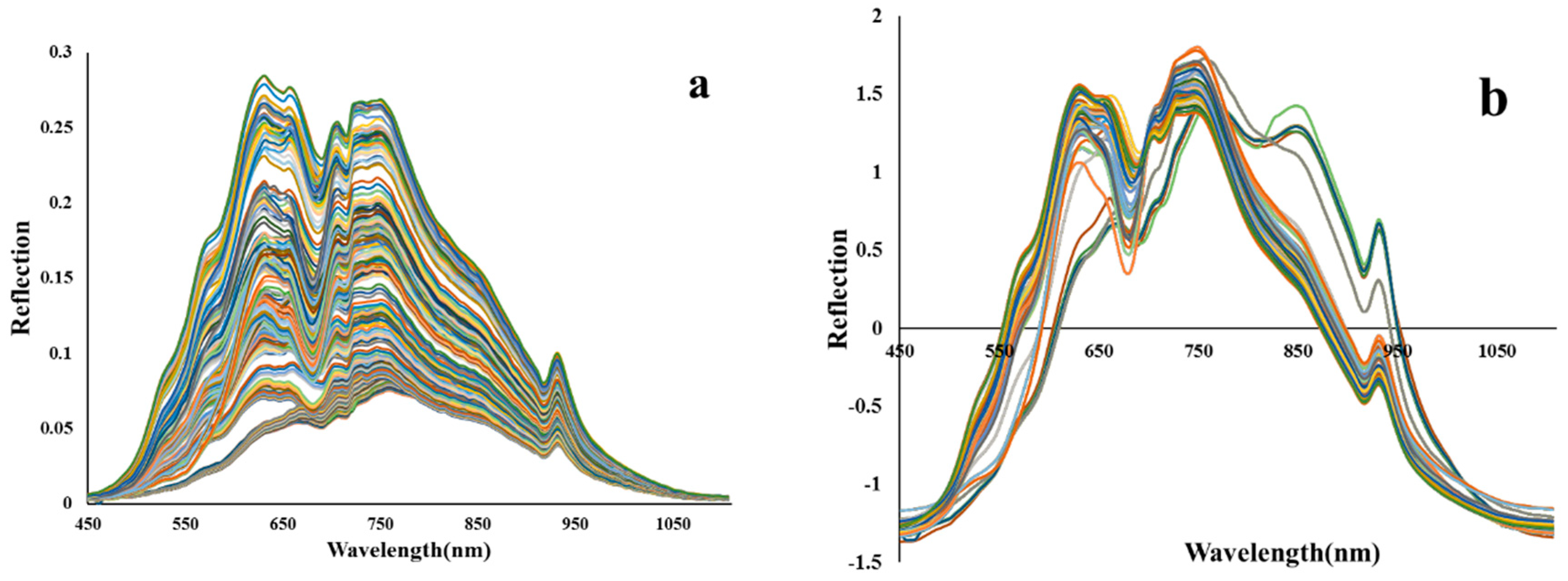
The changes in the spectra of the samples could be due to the chemical and structural properties of the crops; however, spectral curves may be influenced by unwanted factors; i.e. noises. Factors such as stray light, detector noise, changes in the intensity of the ambient light, and temperature variation of the detector, can result in unwanted alterations on the spectral curves [41]. Therefore, spectral pre-processing is the first step in the analysis of these data to eliminate the unwanted factors and further highlight the fine differences between the spectral curves of the samples [42]. Curve smoothing and elimination of the light scattering (normalization) are two common methods in preprocessing the spectra. The purpose of smoothing is to improve the signal-to-noise ratio. Here, the moving average method was adopted to eliminate the random noise and smooth the curves. Using this method, slight and periodic peaks are eliminated, resulting in smoother curves [43,44]. In the second step, standard normal variant (SNV) was used to eliminate the light scattering-induced noise. With the help of this method, the cumulative-increasing effect of light, physical-induced deviation (non-uniform distribution throughout the spectrum, improper sample size, and light refractive index), as well as the changes in the light distance can be resolved. This method further approaches the spectra and highlights their differences [45,46]. The Unscrambler 10.4 was employed for pre-processing of the spectral data. The main and pre-processed spectra of the peanut seeds are depicted in Figure 2.

2.5. Architecture of CNN for classification of HSI images

In the convolution process, a filter/kernel is placed on the input image to achieve a filtered output that includes its main features. The kernel is used in the convolution process to extract the image features. Kernel is a matrix that moves like a window on the input image matrix. Every time it moves, the value of this matrix is multiplied by the input matrix to finally get the desired output [47].

2.5.1. AlexNet architecture

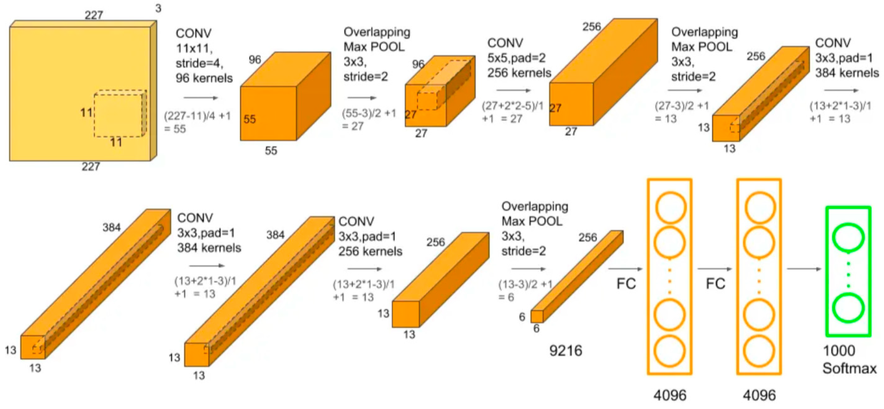
AlexNet is a deep convolutional neural network designed to identify and classify colored images with a size of 224x224x3. In general, this neural network possesses 62 million learning parameters and 11 layers as depicted in Figure 3 [48].
The AlexNet network consists of three types of different layer structures, including convolution layers, pooling layers, and fully connected layers. The convolution layer encompasses a number of filters or kernels, each filter has the duty of extracting certain features from different areas of the image. The first convolutional layer is often used to reduce and eliminate noise, i.e. some pre-processing methods. The subsequent convolutional layers extract the features of the image and check the correlation between different features to provide a feature map. The pooling layer reduces the size of feature maps, which declines the number of learning parameters and the extent of network calculations [50]. The pooling layer summarizes the features of each region of the feature map produced by the convolution layer. In fact, it selects the most important ones and transfers them to the next stage. This makes the model more robustness against changes in the position of the features in the input image. By reducing the size of the input image and summarizing the main and important features in the image, the pooling layer decrements the network computations and the problem of overfitting [51]. The fully connected layers are the last layers of a classification CNN. One of the main uses of the fully connected layer in the convolutional network is its application as a classifier. The set of features extracted by the convolutional layers will finally become a vector. Ultimately, this feature vector is given to a fully connected classifier to identify the correct class [52].

2.5.2. VGG architecture

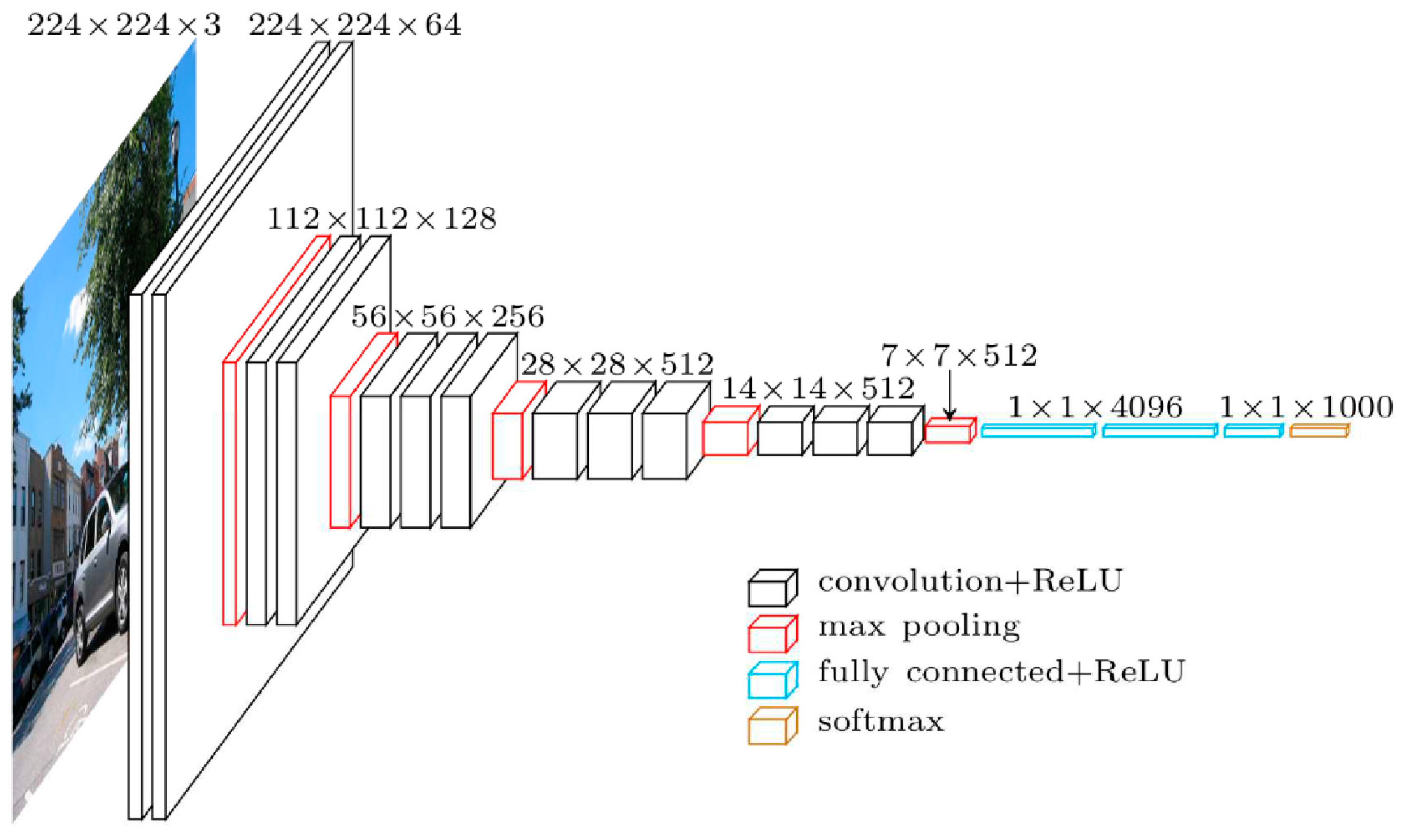
As shown in Figure 4, the VGG network includes 13 convolutional layers or 13 parameter layers. The arrangement of the layers is presented in Figure 4. This network is best known for its pyramid-like form, where layers closer to the image are wider, while those further away are deeper [53]. Convolution layers in this network use small filters (3x3, the smallest possible size for the filter) and also take into account the surrounding pixels. It also has convolutional layers with 1x1 filters, followed by a ReLU activation function [54]. Instead of using the large size filters used (in AlexNet) such as 11x11 or 7x7, In VGGNet utilizes small size filters. This enables the network to have more layers, further improving the network performance. Moreover, VGGNet has less parameters compared to Alexnet. In VGGNet, the number of parameters is 27 times the number of filters, while in AlexNet, this value is 49 times [55]. Furthermore, VGGNet uses 1x1 convolution, which is not present in AlexNet. This network uses 1x1 convolution to increase the nonlinearity of the decision function, but at the same time it does not change the number of filters; That is, the number of filters in the input and output of this convolution is equal [56]. The main drawback of this architecture is that it is very slow and time-consuming if you want to train it from scratch [57]. In this research, WekaDeeplearning4j package have been employed in Weka 3.8.6 software to implement convolutional neural network architectures [58].

2.6. Machine learning techniques for analyzing reflection spectra

2.6.1. Principal component analysis (PCA)

PCA is a transformation in vector space, enabling the analysis of large datasets with a large number of dimensions or features such as spectral data. It also provides the possibility of increasing the interpretability of data by preserving the maximum amount of information and visualizing multidimensional data [59]. PCA is indeed a statistical technique to decline the dimensions of a dataset by linear transformation of the data into a new coordinate system, such that the most variance in the data can be described with smaller dimensions than the original data [60]. In this approach, a linear combination of the initial variables with the highest correlation are used to form a new axis known as principal components (PC). The aim of each PC is to maximize the variance of the data to extract the maximum useful information. PCs are made with no correlation with each other [42]. The first two PCs usually contain the most variance of the data. The data of the same category can be clustered by drawing the data in a two-dimensional graph resulting from these PCs [16]. In this method, the matrix of primary variables (X) is divided into two new matrices called scores and loadings. The scores assigned to each sample in PCs identify the pattern of changes in the data. On the other hand, the weight of the main variables in the structure of PCs is determined using loadings. In this way, signs appear that determine which variables play an important role in the process of data changes [61].

2.6.2. Linear discriminant analysis (LDA)

LDA aims to find a linear separator between classes of objects and use this decision function to assign class membership to unknown samples. Other more complex decision levels (e.g., detecting nonlinear behaviors in quadratic discriminant analysis) also exist which require more parameters to be set [61]. LDA combined to PCA is known as a dimensionality reduction tool. However, in LDA, new axes are formed to maximize the separation of classes [59]. This is achieved by maximizing the distance between the average values of each class while minimizing the dispersion of the dataset in each class. Then the data are mapped to the new axis with a lower dimension [62]. However, LDA should not be used for matrices with more variables than the number of samples, especially in the presence of correlated variables. To resolve this limitation, LDA can be applied to the score matrix (t) obtained after applying PCA while keeping all non-zero principal components [63]. Due to the stability of LDA, it has been widely used to classify agricultural and food products based on hyperspectral data. In most of the studies on the use of LDA for classification by hyperspectral imaging, the average classification precision was reported to be more than 90%, suggesting the stability of the classifier [64,65].

2.6.3. Support vector machine (SVM)

SVM aims to obtain optimal hyperplane (points separating one class from others) through selecting items that cross the largest possible gaps between points of different classes. Then, the new points are classified into a special class depending on the surfaces they fall on. The process of creating an optimal hyperplane reduces the generalization error and thus the chance of overfitting [66]. SVM is specifically effective when dealing with high-dimensional spaces that require learning from multiple features in the problem. SVM is also effective in the cases with relatively small data, that is, a high-dimensional space with few sample points [62]. Moreover, SVM requires lower memory as a subset of points is used only to represent boundary surfaces. However, SVM models involve intensive computations during model training [67]. SVM-based machine learning techniques have been mostly used in the classification of different food products, agricultural products, disease detection, adulteration, seed viability, and quantification of chemical compounds in agricultural materials [68,69]. The use of a small number of PCs obtained from the PCA method instead of a large number of primary variables can greatly improve the classification model [70,71].
In this research, PCA was first employed to reduce the dimensions and decline the complexity. Then, new variables (PCs scores) were used to form methods of seed classification using LDA and SVM. These processes were all implemented in the Unscambler 10.4 software.

2.7. Evaluation criteria of models for peanut seed classification

The statistical criteria of accuracy, precision, sensitivity, specificity, and receiver operating characteristic (ROC) were used to evaluate the precision of peanut seed viability classification models. Accuracy determines how close the measured value is to the true value. Precision shows the closeness of the measurement values (implying constant error in different measurements) for consecutive measurements. Sensitivity reveals the fraction of positive answers that are correctly recognized; while specificity denotes the fraction of negative answers that are correctly detected. The mentioned criteria were calculated using Eqs. (1) to (4) [72]:
Accuracy = True   Positive + True   Negative True   Positive + False   Negative + False   Negative + True   Negative
Precision = True   Positive True   Positive + False   Positive
Sensitivity = True   Positive True   Positive   +   False   Negative
Specificity = True   Negative False   Positive   +   True   Negative
Where in:
True Positive = the number of samples in the i-th category that were correctly recognized by the algorithm.
False Negative = the number of samples in the i-th category that were incorrectly determined by the algorithm.
False Positive=The number of samples outside the i-th category that were placed in the i-th category by the algorithm.
True Negative=The number of samples outside the i-th category that were not placed in the i-th category by the algorithm.

3. Results and Discussion

3.1. Indices of seed viability

Table 2 lists the measurement results and calculated seed viability indices for each cultivar in three time periods. Accordingly, the accelerated aging test caused certain differences in the viability indices of the treatments. In both cultivars, accelerated aging treatment significantly declined the percentage of seed germination. Such that after 24 and 48 hours of incubation, the percentage of seed germination was decreased to 70% and 50%, respectively. Moreover, other seed germination indices significantly decreased after incubation.

3.2. Modeling of seed viability classification based on hyperspectral images using CNN

Table 3 presents the ability of CNN architectures in determining the seeds viability using hyperspectral images. Based on Table 3, both CNN architectures exhibited a high performance in seed classification. However, the VGGNet architecture showed slightly better performance in seed classification which can be attributed to the use of small sized filters rather than large ones used in AlexNet (11×11 or 7×7). As hyperspectral images separately provide spectral data of each pixel to CNN, small size filters can spatially track spectral changes in smaller areas and offer a more thorough analysis of the image [73,74]. On the other hand, the pyramidal architecture of VGGNet enables extracting the general features of the image in the initial layers; by increasing the layers, the spectral-spatial and partial features of the image can also be extracted [75,76]. It seems that the strategy of moving from whole to fraction for extracting image features in VGGNet architecture led to a realistic analysis of spectral-spatial changes. Such a structure, however, has disadvantages for instance, the execution time of VGGNet architecture is somewhat longer than AlexNet [77]. The results of this research were consistent with other studies on the combination of hyperspectral image technology and deep learning to identify the characteristics of agricultural products. AlexNet classifier was used to identify papaya fruit maturity based on hyperspectral images which provided high classification precision [78]. In another work, hyperspectral images with classifier were used to identify sorghum cultivars which also offered high classification precision [79]. Moreover, the efficiency of VGG classification in identifying agricultural products has been investigated in several studies which are in line with results of this research. The CNN-based classifiers such as VGG and AlexNet were used to determine the cultivar of peanut seeds based on the images which showed high classification precision [80]. In another study, CNN-based classifiers such as VGG and AlexNet were employed to classify corn seeds into specific classes, whose results indicated that this type of classifiers combined with spectral images had a high ability to identify the seed classes [30].
Figure 5 and Figure 6 respectively depicts the confusion matrix of AlexNet and VGGNet architectures to offer a comparison between the best and worst classifiers in each treatment. Accordingly, the most incorrect detections were for the determination of the seed cultivar; while the seeds were placed in relatively correct viability classes. Another important point is the better performance of the AlexNet architecture in correct determination of the NC-2 cultivar; while the VGGNet architecture presented better performance in the detection of the Florispan cultivar.

3.3. PC results

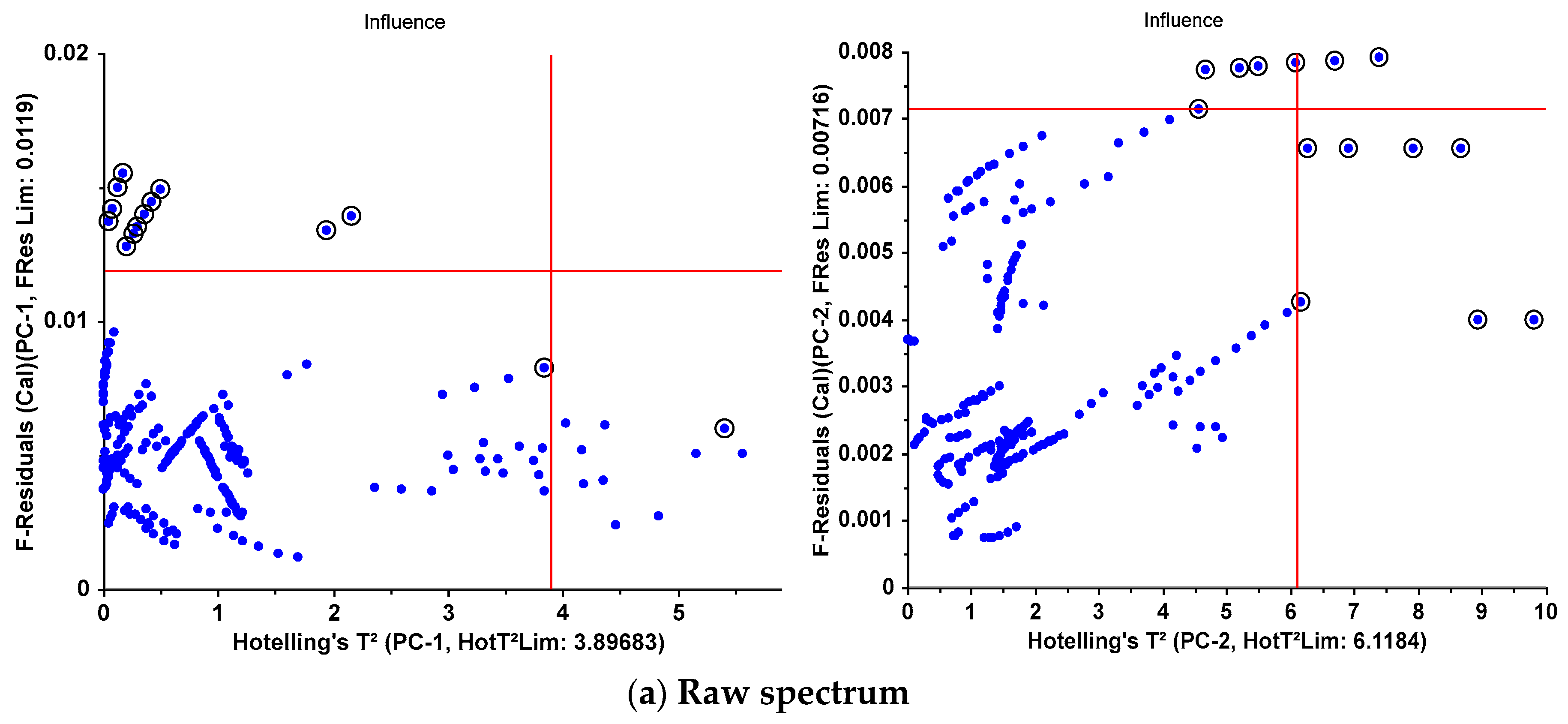
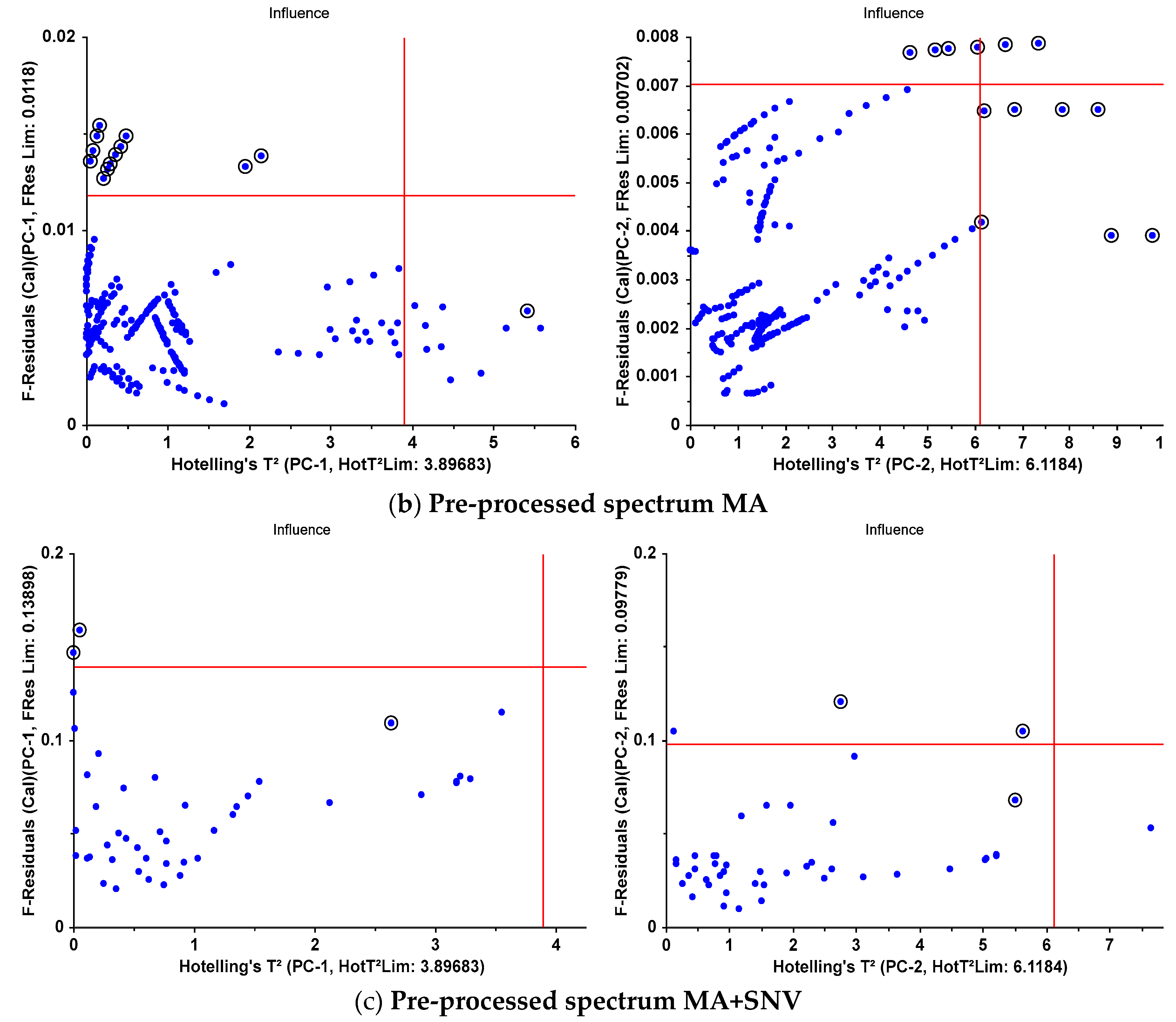
Identification of outliers is a significant and prerequisite step in modeling high-dimensional data (spectral data). By scrutinizing investigation the outlier data, it is possible to decide whether such data will have a negative effect on the performance and accuracy of the model or not, and thus a rule is established to remove them [81]. The outliers are generally observations which do not follow the overall distribution of the data. For two reasons, data may be considered outliers: those that are not well described by the model and have a high residual and data with too much impact on the model including several components to describe that (For two reasons, data may be considered outliers. Data that is not well described by the model and has a high residual; Data that affects the model too much and several components may be included in the model to describe it alone [7]. PCA is a common technique that has been used in several studies to identify outlier data. Leverages-residuals diagram is a powerful tool to identify outliers in PCA [82]. Figure 7 shows the configuration of outliers in the leverage-residual diagram for several pre-processing methods. Table 4 also lists the number of identified outliers and their position in the leverage-residual diagram for different pre-processing methods.
Samples with high residual variance, i.e. in the upper regions of the graph, are poorly described by the model. As long as samples with high residual variance are not influential (Samples with low Hotelling's T²), keeping them in the model may not be problematic (for example, high residual variance may be due to non-significant regions of a spectrum) [83]. But samples with high Hotelling'sT² are better to be removed from the model because even if they have a low residual, the model may be too influenced by them. In such a case, a component may be exclusively included in the model to describe one sample, thus deviating the model from the appropriate path to describe other samples. A sample with high residual variance and high Hotelling's T² is the most dangerous outlier; because it is not only poorly described by the model but it is also influential. Such samples may include several components on their own. Therefore, such samples must be removed from the model [84]. According to Table 4, the number of residual samples in PC1 is more than PC2 and the capacity of PC2 was used to describe these samples. Therefore, elimination of such samples with negligible count can result in a situation in which the capacity of PCs is dedicated to describing a larger set of data rather than describing a few samples, thus, the model provides better generalizability [85]. Another interesting point in Table 4 is that MA+SNV pre-processing showed less outliers compared to the raw data spectrum which can be due to the reduction of unimportant areas of a spectrum and also the elimination of noise from the data.
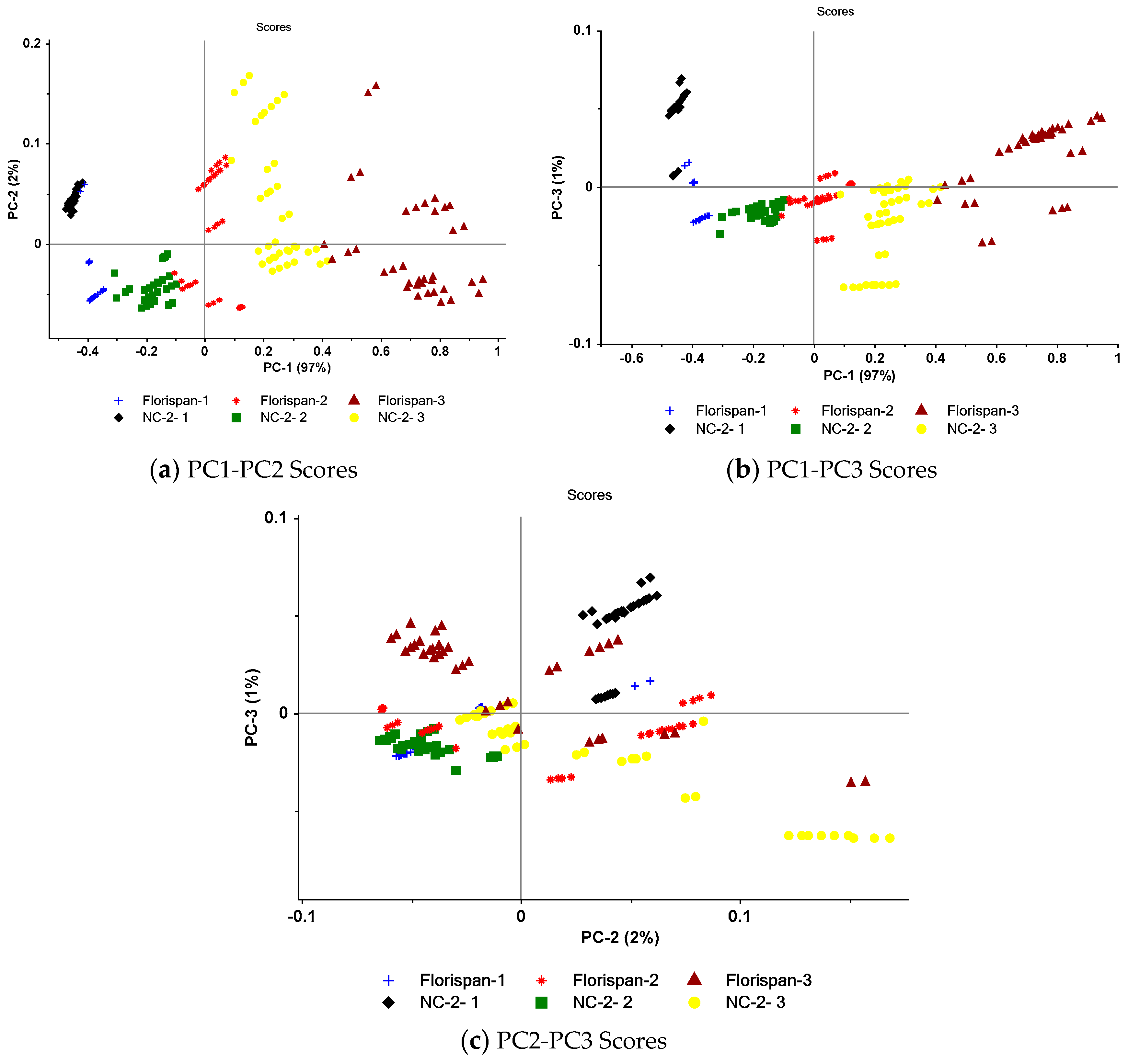
The score curve is plotted in Figure 8 which describes the data structure in terms of sample patterns and generally shows the differences or similarities of the sample.
Samples with close scores along a PC are similar to each other and most likely belong to the same class. This diagram also specifies which PCs (or primary variables) play a greater role in describing a particular sample [86]. Figure 8a is related to PC1-PC2. It is possible to easily identify the seed classes, and in particular, the distinction between seeds with high viability in both cultivars compared to other seeds. The samples had very close scores in the first period of viability, suggesting the similar and uniform properties of the seeds. In the third period, however, the scores of the seeds are somewhat different, indicating non-uniformity and variation of the properties of the seeds over time. According to Figure 8b,c, PC2 and PC3 did not play a significant role in describing the variance of the samples, and it is not possible to distinguish the classes based on the scores of these two PCs. The interesting point in Figure 8 is that the first three PCs can describe 100% of the variance in the samples, hence, these three PCs will be applied to model seed viability using LDA and SVM methods.

3.4. Modeling the seed viability classification based on reflection spectra using LDA and SVM

Table 5 lists the results of evaluating the ability of LDA and SVM techniques in identifying the viability of seeds using reflection spectra. As seen, both techniques have a high performance in seed classification. However, SVM has slightly better performance in seed classification.
Figure 9 and Figure 10 respectively depicts the confusion matrix for LDA and SVM classification, for a clear comparison between the best and worst classifiers in each treatment. Accordingly, both the classifiers showed a good ability to detect the seeds with the first viability (first period) such that the worst diagnosis was related to the samples of the second period. In general, careful examination of the figures shows no significant difference between the predictions of the two methods.
Various machine learning algorithms have been extensively utilized to classify agricultural products based on spectroscopic data. Interestingly, the models did not reach high precision in cases where raw spectra were used for modeling. The precision was greatly improved by adopting pre-processing models, variable selection techniques, and variable extraction method before modeling (prediction of corn seed viability by combining MSC+PCA+SVM methods [87], detection of contaminated cucumber seeds by PLS-DA [88], and prediction of seed viability by PCA+SVM and PCA+CNN [89]. This phenomenon can be assigned to the high amount of noise, excess data, and high-correlated variables of the high-dimensional datasets which make modeling more complicated and time consuming, hence, decrementing the ability of the model to predict new samples. The application of spectral preprocessing followed by PCA technique can eliminate the noise and excess data. By extracting new variables by a combination of the correlated variables, the excess data will be eliminated, decreasing the complexity of the model while incrementing its precision.
Comparing the results of CNN classifiers with LDA and SVM showed no significant difference between the efficiency of these models. However, the important point is that the CNN classification does not require a separate spectral preprocessing and variable extraction. All these steps are implemented in different layers of these classifications. Moreover, pre-trained AlexNet and VGGNet architectures have the capability of direct application on the hyperspectral images to analyze all points of the sample spatially and spectrally. The drawback of processing of HSI with CNN is its high computational burden and time-consuming process compared to the analysis of reflection spectra using LDA and SVM. Therefore, it can be concluded that the processing of hyperspectral images by CNN is more suitable for the cases with spatially varying features such as diseases on the surface of the fruits or detection of bruise on them. On the other hand, analysis of reflection spectra by LDA and SVM methods best suites the cases addressing the overall feature of the sample such as prediction of solid soluble materials, acidity, or viability of the seeds.

4. Conclusions

Evaluation of the seed quality is of crucial significance for the agricultural products. Identification of the seed viability can remarkably affect the product yield. The initial method of seed viability assessment are time consuming, costly, and destructive while lacking the generalizability to the entire seeds. Here, a combination of hyperspectral images with CNN architecture and on the other hand a combination of reflection spectra with LDA and SVM classification methods were used to determine the viability of peanut seeds. The results of this research indicated the high capability of CNN architectures such as AlexNet and CGGNet in determining the seed viability based on hyperspectral images with no preprocessing and separate feature extraction. The accuracy of the mentioned method was 0.985 and 0.986, respectively. Their computational time was, however, longer than the conventional machine learning methods.
The presence of abnormal data with high distance from the general mean value of the data which does not follow the overall trend of the data set can drastically affect the modeling process and disrupt the model performance. Such data are known as outliers. The results of this research indicated that PCA is a powerful method for identification of outliers. Moreover, the application of pre-processing methods such as MA and SNV can remarkably decline the number of outliers by smoothing and noise elimination. Therefore, the inhomogeneity due to the spectral disturbances will be resolved such that the number of outliers declined from 14 before preprocessing to 3 after that. Moreover, a combination of feature extraction method of PCA with LDA and SVM classifications showed that the use of a limited number of PCs instead of all wavelengths can decrement the complexity of modeling while enhancing the efficiency of the models. LDA and SVM classification methods resulted in accuracy of 0.983 and 0.986 in classification of peanut seeds, respectively. Overall, it can be concluded that the processing of hyperspectral images with CNN is appropriate for cases with spatially variable features, for instance detection of diseases on the surface of the fruits or bruise detection on the fruits. On the other hand, analysis of the reflection spectra by LDA and SVM is most suitable for cases addressing the overall feature of the sample for example prediction of solid soluble substances, acidity, or seed viability as well as online applications requiring high-speed processing.

Author Contributions

Conceptualization, M.R.-S., A.M. and M.T.; methodology, M.R.-S., Y.A-G., A.M. and M.T.; software, M.R.-S., A.M. and M.T.; validation, M.R.-S., Y.A-G.; A.M.,; formal analysis Y.A-G.; M.K.; investigation, Y.A-G.; M.R.-S., M.K; resources, M.R.-S., M.K.; data curation, M.R.-S., Y,A-G., writing—original draft preparation, M.R.-S.; A.M. and M.T.; writing—review and editing, Y.A-G., E.D.L.C.-G., M.H.-H., J.L.H.-H.; visualization, M.R.-S.; supervision, Y.A-G.; project administration, Y.A-G.; funding acquisition, Y.A-G.; E.D.L.C.-G., M.H.-H., J.L.H.-H. All authors have read and agreed to the published version of the manuscript.

Funding

This research received no external funding..

Data Availability Statement

The datasets used and/or analyzed during the current study are available from the corresponding author on reasonable request.

Conflicts of Interest

The authors declare that they have no known competing financial interest or personal relationship that could have appeared to influence the work reported in this paper.

References

  1. Yang, H.; Ni, J.; Gao, J.; Han, Z.; Luan, T. A novel method for peanut variety identification and classification by Improved VGG16. Scientific Reports 2021, 11, 15756. [CrossRef]
  2. Zhao, X.; Pang, L.; Wang, L.; Men, S.; Yan, L. Deep Convolutional Neural Network for Detection and Prediction of Waxy Corn Seed Viability Using Hyperspectral Reflectance Imaging. Mathematical and Computational Applications 2022, 27, 109. [CrossRef]
  3. Kandpal, L.M.; Lohumi, S.; Kim, M.S.; Kang, J.-S.; Cho, B.-K. Near-infrared hyperspectral imaging system coupled with multivariate methods to predict viability and vigor in muskmelon seeds. Sensors and Actuators B: Chemical 2016, 229, 534-544. [CrossRef]
  4. Pang, L.; Wang, L.; Yuan, P.; Yan, L.; Yang, Q.; Xiao, J. Feasibility study on identifying seed viability of Sophora japonica with optimized deep neural network and hyperspectral imaging. Computers and Electronics in Agriculture 2021, 190, 106426. [CrossRef]
  5. Kusumaningrum, D.; Lee, H.; Lohumi, S.; Mo, C.; Kim, M.S.; Cho, B.K. Non-destructive technique for determining the viability of soybean (Glycine max) seeds using FT-NIR spectroscopy. Journal of the Science of Food and Agriculture 2018, 98, 1734-1742. [CrossRef]
  6. Shrestha, S.; Knapič, M.; Žibrat, U.; Deleuran, L.C.; Gislum, R. Single seed near-infrared hyperspectral imaging in determining tomato (Solanum lycopersicum L.) seed quality in association with multivariate data analysis. Sensors and Actuators B: Chemical 2016, 237, 1027-1034. [CrossRef]
  7. Wang, X.; Zhang, H.; Song, R.; He, X.; Mao, P.; Jia, S. Non-destructive identification of naturally aged alfalfa seeds via multispectral imaging analysis. Sensors 2021, 21, 5804. [CrossRef]
  8. Marcos Filho, J. Seed vigor testing: an overview of the past, present and future perspective. Scientia agricola 2015, 72, 363-374. [CrossRef]
  9. Song, P.; Kim, G.; Song, P.; Yang, T.; Yue, X.; Gu, Y. Rapid and non-destructive detection method for water status and water distribution of rice seeds with different vigor. International Journal of Agricultural and Biological Engineering 2021, 14, 231-238. [CrossRef]
  10. ElMasry, G.; Mandour, N.; Al-Rejaie, S.; Belin, E.; Rousseau, D. Recent applications of multispectral imaging in seed phenotyping and quality monitoring—An overview. Sensors 2019, 19, 1090. [CrossRef]
  11. de Medeiros, A.D.; Bernardes, R.C.; da Silva, L.J.; de Freitas, B.A.L.; dos Santos Dias, D.C.F.; da Silva, C.B. Deep learning-based approach using X-ray images for classifying Crambe abyssinica seed quality. Industrial Crops and Products 2021, 164, 113378. [CrossRef]
  12. de Medeiros, A.D.; Pinheiro, D.T.; Xavier, W.A.; da Silva, L.J.; dos Santos Dias, D.C.F. Quality classification of Jatropha curcas seeds using radiographic images and machine learning. Industrial Crops and Products 2020, 146, 112162. [CrossRef]
  13. Li, L.; Chen, S.; Deng, M.; Gao, Z. Optical techniques in non-destructive detection of wheat quality: A review. Grain & Oil Science and Technology 2022, 5, 44-57. [CrossRef]
  14. Jia, B.; Wang, W.; Ni, X.; Lawrence, K.C.; Zhuang, H.; Yoon, S.-C.; Gao, Z. Essential processing methods of hyperspectral images of agricultural and food products. Chemometrics and Intelligent Laboratory Systems 2020, 198, 103936. [CrossRef]
  15. Saha, D.; Manickavasagan, A. Machine learning techniques for analysis of hyperspectral images to determine quality of food products: A review. Current Research in Food Science 2021, 4, 28-44. [CrossRef]
  16. Yang, Y.; Zhang, X.; Yin, J.; Yu, X. Rapid and nondestructive on-site classification method for consumer-grade plastics based on portable NIR spectrometer and machine learning. Journal of Spectroscopy 2020, 2020, 1-8. [CrossRef]
  17. Vega Diaz, J.J.; Sandoval Aldana, A.P.; Reina Zuluaga, D.V. Prediction of dry matter content of recently harvested ‘Hass’ avocado fruits using hyperspectral imaging. Journal of the Science of Food and Agriculture 2021, 101, 897-906. [CrossRef]
  18. Ravikanth, L.; Singh, C.B.; Jayas, D.S.; White, N.D. Classification of contaminants from wheat using near-infrared hyperspectral imaging. Biosystems Engineering 2015, 135, 73-86. [CrossRef]
  19. Zhou, S.; Sun, L.; Xing, W.; Feng, G.; Ji, Y.; Yang, J.; Liu, S. Hyperspectral imaging of beet seed germination prediction. Infrared Physics & Technology 2020, 108, 103363. [CrossRef]
  20. Caporaso, N.; Whitworth, M.B.; Fisk, I.D. Near-Infrared spectroscopy and hyperspectral imaging for non-destructive quality assessment of cereal grains. Applied spectroscopy reviews 2018, 53, 667-687. [CrossRef]
  21. Yu, Z.; Fang, H.; Zhangjin, Q.; Mi, C.; Feng, X.; He, Y. Hyperspectral imaging technology combined with deep learning for hybrid okra seed identification. Biosystems Engineering 2021, 212, 46-61. [CrossRef]
  22. Han, S.S.; Kim, M.S.; Lim, W.; Park, G.H.; Park, I.; Chang, S.E. Classification of the clinical images for benign and malignant cutaneous tumors using a deep learning algorithm. Journal of Investigative Dermatology 2018, 138, 1529-1538. [CrossRef]
  23. Huang, Q.; Li, W.; Zhang, B.; Li, Q.; Tao, R.; Lovell, N.H. Blood cell classification based on hyperspectral imaging with modulated Gabor and CNN. IEEE journal of biomedical and health informatics 2019, 24, 160-170. [CrossRef]
  24. Zhao, W.; Du, S. Spectral–spatial feature extraction for hyperspectral image classification: A dimension reduction and deep learning approach. IEEE Transactions on Geoscience and Remote Sensing 2016, 54, 4544-4554. [CrossRef]
  25. Sony, S.; Dunphy, K.; Sadhu, A.; Capretz, M. A systematic review of convolutional neural network-based structural condition assessment techniques. Engineering Structures 2021, 226, 111347. [CrossRef]
  26. Chen, L.; Li, S.; Bai, Q.; Yang, J.; Jiang, S.; Miao, Y. Review of image classification algorithms based on convolutional neural networks. Remote Sensing 2021, 13, 4712. [CrossRef]
  27. Ghosh, A.; Sufian, A.; Sultana, F.; Chakrabarti, A.; De, D. Fundamental concepts of convolutional neural network. Recent trends and advances in artificial intelligence and Internet of Things 2020, 519-567. [CrossRef]
  28. Kabir, M.H.; Guindo, M.L.; Chen, R.; Liu, F.; Luo, X.; Kong, W. Deep Learning Combined with Hyperspectral Imaging Technology for Variety Discrimination of Fritillaria thunbergii. Molecules 2022, 27, 6042. [CrossRef]
  29. Yang, Y.; Liao, J.; Li, H.; Tan, K.; Zhang, X. Identification of high-oil content soybean using hyperspectral reflectance and one-dimensional convolutional neural network. Spectroscopy Letters 2023, 56, 28-41. [CrossRef]
  30. Ma, X.; Li, Y.; Wan, L.; Xu, Z.; Song, J.; Huang, J. Classification of seed corn ears based on custom lightweight convolutional neural network and improved training strategies. Engineering Applications of Artificial Intelligence 2023, 120, 105936. [CrossRef]
  31. Wang, Y.; Song, S. Variety identification of sweet maize seeds based on hyperspectral imaging combined with deep learning. Infrared Physics & Technology 2023, 130, 104611. [CrossRef]
  32. Boulent, J.; Foucher, S.; Théau, J.; St-Charles, P.-L. Convolutional neural networks for the automatic identification of plant diseases. Frontiers in plant science 2019, 10, 941. [CrossRef]
  33. De Vitis, M.; Hay, F.R.; Dickie, J.B.; Trivedi, C.; Choi, J.; Fiegener, R. Seed storage: maintaining seed viability and vigor for restoration use. Restoration Ecology 2020, 28, S249-S255. [CrossRef]
  34. Zou, Z.; Chen, J.; Zhou, M.; Zhao, Y.; Long, T.; Wu, Q.; Xu, L. Prediction of peanut seed vigor based on hyperspectral images. Food Science and Technology 2022, 42, e32822. [CrossRef]
  35. Hampton, J.G.; TeKRONY, D.M. Handbook of vigour test methods; The International Seed Testing Association, Zurich (Switzerland). 1995.
  36. Moghaddam, M.; Moradi, A.; Salehi, A.; Rezaei, R. The effect of various biological treatments on germination and some seedling indices of fennel (Foeniculum vulgare L.) under drought stress. Iranian Journal of Seed Science and Technology 2018, 7.
  37. Panwar, P.; Bhardwaj, S. Handbook of practical forestry; Agrobios (India): 2005.
  38. Mohajeri, F.; Taghvaei, M.; Ramrudi, M.; Galavi, M. Effect of priming duration and concentration on germination behaviors of (Phaseolus vulgaris L.) seeds. Int. J. Ecol. Environ. Conserv 2016, 22, 603-609.
  39. Maguire, J.D. Speed of germination-aid in selection and evaluation for seedling emergence and vigor. Crop Sci. 1962, 2, 176-177. [CrossRef]
  40. Hunter, E.; Glasbey, C.; Naylor, R. The analysis of data from germination tests. The Journal of Agricultural Science 1984, 102, 207-213. [CrossRef]
  41. Jiao, Y.; Li, Z.; Chen, X.; Fei, S. Preprocessing methods for near-infrared spectrum calibration. Journal of Chemometrics 2020, 34, e3306. [CrossRef]
  42. Xu, Y.; Zhong, P.; Jiang, A.; Shen, X.; Li, X.; Xu, Z.; Shen, Y.; Sun, Y.; Lei, H. Raman spectroscopy coupled with chemometrics for food authentication: A review. TrAC Trends in Analytical Chemistry 2020, 131, 116017. [CrossRef]
  43. Roger, J.-M.; Mallet, A.; Marini, F. preprocessing NIR spectra for aquaphotomics. Molecules 2022, 27, 6795. [CrossRef]
  44. Suhandy, D.; Yulia, M. The use of UV spectroscopy and SIMCA for the authentication of Indonesian honeys according to botanical, entomological and geographical origins. Molecules 2021, 26, 915. [CrossRef]
  45. Cozzolino, D.; Williams, P.; Hoffman, L. An overview of pre-processing methods available for hyperspectral imaging applications. Microchemical Journal 2023, 109129. [CrossRef]
  46. Saha, D.; Senthilkumar, T.; Sharma, S.; Singh, C.B.; Manickavasagan, A. Application of near-infrared hyperspectral imaging coupled with chemometrics for rapid and non-destructive prediction of protein content in single chickpea seed. Journal of Food Composition and Analysis 2023, 115, 104938. [CrossRef]
  47. Ajit, A.; Acharya, K.; Samanta, A. A Review of Convolutional Neural Networks. In Proceedings of 2020 International Conference on Emerging Trends in Information Technology and Engineering (ic-ETITE), Vellore, India; pp. 1-9. [CrossRef]
  48. Lv, M.; Zhou, G.; He, M.; Chen, A.; Zhang, W.; Hu, Y. Maize leaf disease identification based on feature enhancement and DMS-robust alexnet. IEEE access 2020, 8, 57952-57966. [CrossRef]
  49. Tan, Y.; Jing, X. Cooperative spectrum sensing based on convolutional neural networks. Applied Sciences 2021, 11, 4440. [CrossRef]
  50. Sakib, S.; Ahmed, N.; Kabir, A.J.; Ahmed, H. An overview of convolutional neural network: Its architecture and applications. 2019. [CrossRef]
  51. Li, Z.; Liu, F.; Yang, W.; Peng, S.; Zhou, J. A survey of convolutional neural networks: analysis, applications, and prospects. IEEE transactions on neural networks and learning systems 2021. [CrossRef]
  52. Naranjo-Torres, J.; Mora, M.; Hernández-García, R.; Barrientos, R.J.; Fredes, C.; Valenzuela, A. A review of convolutional neural network applied to fruit image processing. Applied Sciences 2020, 10, 3443. [CrossRef]
  53. Gebrehiwot, A.; Hashemi-Beni, L.; Thompson, G.; Kordjamshidi, P.; Langan, T.E. Deep convolutional neural network for flood extent mapping using unmanned aerial vehicles data. Sensors 2019, 19, 1486. [CrossRef]
  54. Simonyan, K.; Zisserman, A. Very deep convolutional networks for large-scale image recognition. arXiv preprint arXiv:1409.1556 2014. [CrossRef]
  55. Yu, W.; Yang, K.; Bai, Y.; Xiao, T.; Yao, H.; Rui, Y. Visualizing and comparing AlexNet and VGG using deconvolutional layers. In Proceedings of Proceedings of the 33 rd International Conference on Machine Learning.
  56. Alsaadi, Z.; Alshamani, E.; Alrehaili, M.; Alrashdi, A.A.D.; Albelwi, S.; Elfaki, A.O. A real time Arabic sign language alphabets (ArSLA) recognition model using deep learning architecture. Computers 2022, 11, 78. [CrossRef]
  57. Khalifa, N.E.M.; Taha, M.H.N.; Hassanien, A.E. Aquarium family fish species identification system using deep neural networks. In Proceedings of International Conference on Advanced Intelligent Systems and Informatics; pp. 347-356. [CrossRef]
  58. Lang, S.; Bravo-Marquez, F.; Beckham, C.; Hall, M.; Frank, E. Wekadeeplearning4j: A deep learning package for weka based on deeplearning4j. Knowledge-Based Systems 2019, 178, 48-50. [CrossRef]
  59. Neo, E.R.K.; Yeo, Z.; Low, J.S.C.; Goodship, V.; Debattista, K. A review on chemometric techniques with infrared, Raman and laser-induced breakdown spectroscopy for sorting plastic waste in the recycling industry. Resources, Conservation and Recycling 2022, 180, 106217. [CrossRef]
  60. Park, H.; Son, J.-H. Machine learning techniques for THz imaging and time-domain spectroscopy. Sensors 2021, 21, 1186. [CrossRef]
  61. Peris-Díaz, M.D.; Krężel, A. A guide to good practice in chemometric methods for vibrational spectroscopy, electrochemistry, and hyphenated mass spectrometry. TrAC Trends in Analytical Chemistry 2021, 135, 116157. [CrossRef]
  62. Raschka, S.; Mirjalili, V. Python machine learning Packt Publishing Ltd. 2015.
  63. Brereton, R.G.; Lloyd, G.R. Partial least squares discriminant analysis: taking the magic away. Journal of Chemometrics 2014, 28, 213-225. [CrossRef]
  64. Qin, J.; Vasefi, F.; Hellberg, R.S.; Akhbardeh, A.; Isaacs, R.B.; Yilmaz, A.G.; Hwang, C.; Baek, I.; Schmidt, W.F.; Kim, M.S. Detection of fish fillet substitution and mislabeling using multimode hyperspectral imaging techniques. Food Control 2020, 114, 107234. [CrossRef]
  65. Delwiche, S.R.; Rodriguez, I.T.; Rausch, S.; Graybosch, R. Estimating percentages of fusarium-damaged kernels in hard wheat by near-infrared hyperspectral imaging. Journal of Cereal Science 2019, 87, 18-24. [CrossRef]
  66. Meza Ramirez, C.A.; Greenop, M.; Ashton, L.; Rehman, I.U. Applications of machine learning in spectroscopy. Applied Spectroscopy Reviews 2021, 56, 733-763. [CrossRef]
  67. Zhang, D.; Zhang, H.; Zhao, Y.; Chen, Y.; Ke, C.; Xu, T.; He, Y. A brief review of new data analysis methods of laser-induced breakdown spectroscopy: machine learning. Applied Spectroscopy Reviews 2022, 57, 89-111. [CrossRef]
  68. Bonah, E.; Huang, X.; Yi, R.; Aheto, J.H.; Yu, S. Vis-NIR hyperspectral imaging for the classification of bacterial foodborne pathogens based on pixel-wise analysis and a novel CARS-PSO-SVM model. Infrared Physics & Technology 2020, 105, 103220. [CrossRef]
  69. Pan, T.-t.; Chyngyz, E.; Sun, D.-W.; Paliwal, J.; Pu, H. Pathogenetic process monitoring and early detection of pear black spot disease caused by Alternaria alternata using hyperspectral imaging. Postharvest Biology and Technology 2019, 154, 96-104. [CrossRef]
  70. Liu, Y.; Nie, F.; Gao, Q.; Gao, X.; Han, J.; Shao, L. Flexible unsupervised feature extraction for image classification. Neural Networks 2019, 115, 65-71. [CrossRef]
  71. Chu, X.; Wang, W.; Ni, X.; Li, C.; Li, Y. Classifying maize kernels naturally infected by fungi using near-infrared hyperspectral imaging. Infrared Physics & Technology 2020, 105, 103242. [CrossRef]
  72. Dhakate, P.P.; Patil, S.; Rajeswari, K.; Abin, D. Preprocessing and Classification in WEKA using different classifiers. Inter J Eng Res Appl 2014, 4, 91-93.
  73. Muhammad, U.; Wang, W.; Chattha, S.P.; Ali, S. Pre-trained VGGNet architecture for remote-sensing image scene classification. In Proceedings of 2018 24th International Conference on Pattern Recognition (ICPR); pp. 1622-1627. [CrossRef]
  74. Saleem, M.H.; Potgieter, J.; Arif, K.M. Plant disease detection and classification by deep learning. Plants 2019, 8, 468. [CrossRef]
  75. Sharma, S.; Guleria, K. Deep learning models for image classification: comparison and applications. In Proceedings of 2022 2nd International Conference on Advance Computing and Innovative Technologies in Engineering (ICACITE); pp. 1733-1738. [CrossRef]
  76. Ullah, A.; Anwar, S.M.; Bilal, M.; Mehmood, R.M. Classification of arrhythmia by using deep learning with 2-D ECG spectral image representation. Remote Sensing 2020, 12, 1685. [CrossRef]
  77. Kolla, M.; Venugopal, T. Efficient classification of diabetic retinopathy using binary cnn. In Proceedings of 2021 International conference on computational intelligence and knowledge economy (ICCIKE); pp. 244-247. [CrossRef]
  78. Garillos-Manliguez, C.A.; Chiang, J.Y. Multimodal deep learning and visible-light and hyperspectral imaging for fruit maturity estimation. Sensors 2021, 21, 1288. [CrossRef]
  79. Bu, Y.; Jiang, X.; Tian, J.; Hu, X.; Han, L.; Huang, D.; Luo, H. Rapid nondestructive detecting of sorghum varieties based on hyperspectral imaging and convolutional neural network. Journal of the Science of Food and Agriculture 2023, 103, 3970-3983. [CrossRef]
  80. Yang, J.; Sun, L.; Xing, W.; Feng, G.; Bai, H.; Wang, J. Hyperspectral prediction of sugarbeet seed germination based on gauss kernel SVM. Spectrochimica Acta Part A: Molecular and Biomolecular Spectroscopy 2021, 253, 119585. [CrossRef]
  81. Hubert, M.; Reynkens, T.; Schmitt, E.; Verdonck, T. Sparse PCA for high-dimensional data with outliers. Technometrics 2016, 58, 424-434. [CrossRef]
  82. Mejia, A.F.; Nebel, M.B.; Eloyan, A.; Caffo, B.; Lindquist, M.A. PCA leverage: outlier detection for high-dimensional functional magnetic resonance imaging data. Biostatistics 2017, 18, 521-536. [CrossRef]
  83. Rafajłowicz, E.; Steland, A. The Hotelling—Like T^ 2 T 2 Control Chart Modified for Detecting Changes in Images having the Matrix Normal Distribution. In Proceedings of Stochastic Models, Statistics and Their Applications: Dresden, Germany, March 2019 14; pp. 193-206. [CrossRef]
  84. Camacho-Tamayo, J.H.; Forero-Cabrera, N.M.; Ramírez-López, L.; Rubiano, Y. Near-infrared spectroscopic assessment of soil texture in an oxisol of the eastern plains of Colombia. Colombia Forestal 2017, 20, 5-18.
  85. Chen, X.; Zhang, B.; Wang, T.; Bonni, A.; Zhao, G. Robust principal component analysis for accurate outlier sample detection in RNA-Seq data. Bmc Bioinformatics 2020, 21, 1-20. [CrossRef]
  86. Lörchner, C.; Horn, M.; Berger, F.; Fauhl-Hassek, C.; Glomb, M.A.; Esslinger, S. Quality control of spectroscopic data in non-targeted analysis–Development of a multivariate control chart. Food Control 2022, 133, 108601. [CrossRef]
  87. Pang, L.; Men, S.; Yan, L.; Xiao, J. Rapid vitality estimation and prediction of corn seeds based on spectra and images using deep learning and hyperspectral imaging techniques. Ieee Access 2020, 8, 123026-123036. [CrossRef]
  88. Lee, H.; Kim, M.S.; Lim, H.-S.; Park, E.; Lee, W.-H.; Cho, B.-K. Detection of cucumber green mottle mosaic virus-infected watermelon seeds using a near-infrared (NIR) hyperspectral imaging system: Application to seeds of the “Sambok Honey” cultivar. Biosystems Engineering 2016, 148, 138-147. [CrossRef]
  89. Ma, T.; Tsuchikawa, S.; Inagaki, T. Rapid and non-destructive seed viability prediction using near-infrared hyperspectral imaging coupled with a deep learning approach. Computers and Electronics in Agriculture 2020, 177, 105683. [CrossRef]
Figure 1. Normal and hyperspectral representation of peanut samples.
Preprints 91360 g001
Figure 2. Vis/NIR spectra of a) raw sample, b) MA+SNV-preprocessed spectrum.
Preprints 91360 g002
Figure 3. The general structure of the AlexNet network [49].
Preprints 91360 g003
Figure 4. VGG network architecture [56].
Preprints 91360 g004
Figure 5. confusion matrix for AlexNet architecture.
Preprints 91360 g005
Figure 6. confusion matrix for VGGNet architecture.
Preprints 91360 g006
Figure 7. Leverage-residual diagram for PC1 and PC2.
Preprints 91360 g007aPreprints 91360 g007b
Figure 8. Data scores for the first three PCs.
Preprints 91360 g008
Figure 9. confusion matrix for SVM classifier.
Preprints 91360 g009
Figure 10. confusion matrix for LDA classifier.
Preprints 91360 g010
Table 1. Equations used to calculate the indices.
The studied index Equation References
Germination Energy G E = M C G P N × 100 [36]
Germination Value G V = M D G × P V [35]
Germination Vigour G V I = G P × M e a n P L + P R 100 [37]
Allometric Coefficien A C = P L P R [38]
Daily Germination Speed D G S = 1 M D G [39]
Mean Daily Germination M D G = G P T [40]
Table 2. Viability indices of peanut seeds.
Variety Period Number Germination percentage Germination Energy Mean Daily Germination Germination Value Daily Germination Speed Simple vitality index
NC-2 1 100 91 86 11.3750 250.2500 0.0879 7.0752
NC-2 2 100 69 61 8.6250 146.6250 0.1159 3.7826
NC-2 3 100 47 34 5.8750 64.6250 0.1702 0.9795
Florispan 1 100 94 92 11.7500 329.0000 0.0851 9.5836
Florispan 2 100 72 63 9.000 153.0000 0.1111 4.0761
Florispan 3 100 52 65 6.5000 84.5000 0.1538 2.0072
Table 3. Results of CNN architecture for determination of the seed age.
Network architecture Accuracy Precision Sensitivity Specificity ROC Area Execution time
AlexNet 0.985 0.955 0.954 0.991 0.992 2153 (s)
VGGNet 0.986 0.959 0.958 0.992 0.981 2356 (s)
Table 4. Outliers detected based on pre-processing method.
Statistical criteria Pre-processing method
Raw MA MA+SNV
PC1 PC2 PC1 PC2 PC1 PC2
F-Residuals 13 4 12 3 2 2
Hotelling’sT² 1 7 1 7 1 1
both 0 3 0 3 0 0
F-Residuals: describe the sample distance to model; Hotelling’sT²: describe how well the sample is described by the model.; Both: Samples located in both critical areas.
Table 5. The results of seed classification based on the variables obtained from the PCA method.
Network architecture Accuracy Precision Sensitivity Specificity ROC Area
SVM-PC 0.986 0.959 0.958 0.991 0.970
LDA-PC 0.983 0.952 0.950 0.990 0.997
Disclaimer/Publisher’s Note: The statements, opinions and data contained in all publications are solely those of the individual author(s) and contributor(s) and not of MDPI and/or the editor(s). MDPI and/or the editor(s) disclaim responsibility for any injury to people or property resulting from any ideas, methods, instructions or products referred to in the content.
Copyright: This open access article is published under a Creative Commons CC BY 4.0 license, which permit the free download, distribution, and reuse, provided that the author and preprint are cited in any reuse.
Prerpints.org logo

Preprints.org is a free preprint server supported by MDPI in Basel, Switzerland.

Subscribe

© 2024 MDPI (Basel, Switzerland) unless otherwise stated