
Submitted:
25 November 2023
Posted:
28 November 2023
You are already at the latest version
Abstract
Modelling and presenting mathematical relationships for human behaviour is one of the most complex issues that researchers have always dealt with. In this article, a bottom-up framework for calculating agricultural needs is presented using the socioeconomic characteristics of farmers (such as education level, age, and dependence on income on agriculture) and how their lands are located concerning each other (interactions between neighbours). The objective function of this framework is to maximize the profit of individual farmers based on the amount of water received. Two scenarios, ABM1 (not considering neighbourhood effects) and ABM2 (all cases of farmers' placement and feeling neighbourhood effects), were investigated. In the first scenario (ABM1), there was a noteworthy reduction in water deficit volumes by approximately 35%, accompanied by a 20% increment in farmers' profits. Interestingly, higher risk-taking tendencies correlated with reduced profit margins. The second scenario (ABM2) underscored the significant role of neighborhood dynamics in cultivating diverse behavioral patterns among farmers, subsequently affecting their profitability. A granular examination revealed that farmers with a higher propensity for risk-taking generally accrued lower profits. Additionally, the study facilitated the calculation of total annual profits and average water consumption for each farmer, offering valuable insights for optimizing water resource management and allocation strategies. These findings are instrumental for planners and water resource managers aiming to promote sustainable agricultural practices and efficient water use.
Keywords:
Agriculture Demand
; Agricultural Risk
; Agent-Based Model
; Standard Operating Policy
1. Introduction
The lack of water in the last few decades has made the water supply issue one of the main limiting factors in the comprehensive development of watersheds now and in the future. In the meantime, the agricultural sector is considered the leading consumer of water resources, consuming the most extractable water [1,2]. Understanding farmers’ behavior may offer assistance to diminish existing pressures on water assets and increment sustainability and versatility to climate change [3,4]. So far, many m have been done regarding the models of water allocation to farmers, which can be referred to as Systems Dynamics (SDs) models [5,6], allocations based on game theory [7,8], allocations based on single or multi-objective optimization algorithms [9,10,11,12], and DPSIR models [13,14]. Each of these methods has specific limitations and strengths. The purpose of this article is to present a behavior model of farmers based on the amount of available water.
Agent-Based Model (ABM) is a relatively new approach to modelling systems composed of independent but interacting factors. Engineering and management sciences jointly seek to model the real world to describe, understand and manage phenomena, with the difference that engineering sciences model natural world phenomena and management sciences model human systems [15,16]. Since the knowledge of modelling in the field of natural phenomena and related laws has advanced a lot, many approximate models have been made for such phenomena, and the effectiveness of these models is evident and provable due to the continuous progress in engineering and physics sciences [17,18]. However, the natural human world is less presented in the form of a model due to the complexities of human behaviour. Also, human systems are much more dynamic and complex than the natural world and do not have a stable state. This causes the complexity and uncertainty of human issues more and more. To decide on how to model them, key factors, rules of behaviour of agents, how agents interact with each other and with the environment, and such issues must be considered [19].
In ABM, computational modelling is done from the bottom up. ABM involves representing individuals in a complex adaptive system as discrete agents interacting autonomously in a simulated space to produce emergent and non-intuitive outcomes at the population level [20]. Agents interact or communicate based on predefined “rules ” [21]. As the rules that govern agents’ behavior influence results, it is imperative to tightly couple all rule-based algorithms throughout the model development process. In addition to other programming languages (such as C, Java, and Python), ABM can be implemented using specialized toolkits such as NetLogo, Swarm, or Repast. ABM is generally based on incremental modeling, starting with a simple model and progressing to more complex models [22].
SDs use loops, stores and flows to model the behaviour of complex systems over time and deal with internal causal loops and time delays that affect the behaviour of the entire system; it is an approach for modelling and simulating systems using ordinary differential equations [23]. ABM refers to modelling in which a dynamic process of interactions between agents is simulated repeatedly over time, similar to what is used in SD and discrete event modelling or other types of simulation methods that happen traditionally [24,25]. The SDs have many problems, and the ABMs should help to solve these problems; although this does not mean that SD is weaker than the ABM, perhaps the SD is much more mature than the ABM, which is still in its early stages [15,26]. The comparison with more details of the two methods is shown in Figure 1. As shown in Figure 1, the main difference between the two methods is in the level of modelling and perspective, which is macro and top-down for SD, but in ABM, they are micro and bottom-up.
The application of ABMs in natural resource sciences was first studied by Bousquet et al. on managing renewable resources. In the mentioned study, a multi-agent simulator was created to better understand the interaction between users and natural resources [28]. Also, Balmann used these models in the field of managing agricultural operations. The research mentioned above focused more on the economic aspects of agriculture, and the most significant financial benefit for farmers was considered [29]. Becu et al. conducted a study in the field of ABM for water management in the catchment area in southern Thailand. For this purpose, they prepared an agent-based model, CATCHSCAPE, and investigated economic scenarios, land use and water resource management [30]. Linkola et al. developed an ABM for drinking water management, and their research showed that by using ABMs, results can be obtained that are difficult to achieve using methods such as SDs and other models [31]. In the field of water quality in the catchment area under the influence of agricultural pollution in a region, a study has been conducted using ABMs, the results of which showed that changing the behaviour of farmers is influential on the prediction and decision-making of other farmers, and the results of the agents’ reactions on Water sources are different [32].
In this paper, we present a framework for agricultural demand that relies on farmers’ socioeconomic characteristics to drive demand. This method exploits the heterogeneity of farmers with respect to age, income, education level, risk-taking, and the maintenance and updating of their memories. Psychological studies of agricultural systems are used to illustrate socioeconomic characteristics of farmers [33,34,35,36]. In the materials and methods section, the general framework of the proposed model is presented, and then two hypothetical scenarios are implemented by this model. Since the number of parameters introduced in the materials and methods section is large, all parameters are given in the abbreviation section along with the corresponding unit.
2. Materials and Methods
Agents involved in this research include farmers and reservoir operators. The decisions that farmers make according to their objective (here is to maximize the profit received from the sale of their products) change the water demand and force the reservoir operator to release according to the water demand. In this study, allocation is based on SOP (Standard Operating Policy). The decisions that farmers make based on their background and circumstances are explained in the following sections.
2.1. Farmers’ Features
The farmers’ decision to select the type of cultivation is influenced by various factors, with age and level of education being considered significant determinants [37,38,39]. Based on studies on agricultural risk [33,34,36,40], the parameter is defined as Equation (1), which shows the level of risk-taking of farmers.
2.2. Neighbourhood
Farmers’ decisions affect each other. To limit the impact of other farmers’ decisions on a farmer, a neighbourhood, according to Figure 2, is considered for each field (or farmer). The reason for the maximum distance of 6 meters in Figure 2 is that the farmers’ land may be partially connected, and the access road is located between them. As shown in Figure 1, polygons 7, 8, 12, 14, 17, and 18 are neighbors around farmer 13. The NF parameter is defined as the number of farmers neighbours a farmer.
2.3. Farmers’ Decisions
In this study, farmers can make three choices: changing the cropping pattern and the cultivation date and improving the irrigation technology. These choices are among the Farmers’ features, as explained in the previous sections.
2.4. Formulation
According to [41], Ω1, Ω2, Ω3 and Ω4 (Equations (2)–(5)) are the parameters that determine what choices the farmer makes in the short and long term based on their past decisions. Their neighbours influence the decisions that each farmer makes. Therefore, a set of neighbours is considered for each farmer. The initial conditions for farmers remain unchanged for the first five years in the model, with modifications being implemented from the fifth year onwards.
The economic evaluation of short-term and long-term decisions made by individual farmers in comparison to their neighbours is demonstrated by Ω1 and Ω2, respectively. If a farmer has earned more profit than their neighbours in the past five years, Ω1 (or Ω2) is assigned a value of 1. Otherwise, it is set to a value of zero.
Ω3 (Ω4) denotes the evaluation regarding the precision of their short-term water estimation concerning their long-term estimations. To illustrate, if the ratio of requested water to available water for each farmer is lower than the corresponding ratio observed in the past five years, Ω3 (Ω4) is assigned a value of 1; otherwise, it is assigned a value of zero. and calculate based on Equations (6)–(8).
The actual yield value (Ya) is obtained based on Equation (9), where Ky and Yp are yield response factor and potential yield (ton/ha), respectively.
The profit of each farmer in the yth year is obtained according to Equation (10), which is equal to the income from the sale of products minus the costs, including the costs of planting and irrigation and, harvesting and changing the irrigation technology if necessary.
2.4.1. Changing the Cropping Pattern
The calculation of the summation of Ω values, denoted as , determines whether a farmer’s demand for water would exceed the average available amount. The violation rate, referred to as β (Equation (11)), represents the farmer’s perception of the water quantity at their disposal [42].
The amount of water expected by each farmer () is obtained from Equation (12). In this article, the amount of water rights for each land is given based on its area (Ai) (so this equation can be changed according to the way water is distributed among farmers). In this equation, the amount of water released in each month is shown by the parameter () and the irrigation efficiency in each year for each farmer is shown by the symbol ().
The method of changing the planting date or changing the planting pattern is that no farmer changes his planting date or pattern in the first 5 years. In the following years, , , are calculated based on the last 5 years. Then the expected water () is calculated based on Equation (12) and the farmer decides according to it what cropping pattern and date to have, and this choice is based on maximizing the profit of each farmer in the same year (Maximizing Equation (10)).
2.4.2. Installing New Irrigation Technology
Creating new ideas in a group of people is a step-by-step process. This means learning about the new thing, what you think about it, deciding what to do, making it happen, and ensuring it works [43]. In the search phase to obtain information about new irrigation technology, alpha parameters, education level and water deficit in the last 5 years are suggested. According to Table 1, if the amount of water deficit in the last 5 years is more than the limit presented in the table (δ1-δ8), the farmer will seek information about new irrigation technology.
To simplify the problem, the next step after acquiring knowledge is to decide on the use of new irrigation technology (Table 2). The items in the table + mean the farmer’s decision to use the new irrigation technology.
The flowchart of the proposed model is shown in Figure 3. As is evident in the figure, at the end, the profit and the amount of agricultural demand in the studied period can be calculated. The ABM simulator shown in the middle of the flowchart determines how agricultural demand will change each year.
2.5. Model testing
The hypothetical study area includes 30,000 hectares of agricultural land, which is equally divided among 15 farmers with different ages and educational characteristics. Figure 4 shows the initial agricultural lands site plan. The dominant cultivation in this area is assumed to include four crops: wheat, barley, cucumber and tomato. At first, it is assumed that every 15 farmers cultivate all four crops equally. The characteristics of the 15 farmers considered in this section are given in Table 3. The α parameter, which is the main foundation of this study, was tried to be completely scattered.
β was considered 0.6 for the old irrigation technology and 0.8 for the new technology and ITC was considered 14 million dollars for each land. Also, the values of δ1 to δ4 were considered 30, 25, 20 and 15, and δ5 to δ8 35, 30, 25, 20, respectively. Crops agronomic characteristics (CD (m3/ha), Yp (ton/ha), Ky) and cost and sale of products (Cc (($/ha)) and Sc ($/Kg)) were given from our last published research, which was done downstream of the Karaj reservoir dam. In this study, bringing forward and postponing the cultivation date was considered 7, 14, 21, and 28 days [44].
The defined problem was investigated in two scenarios. In ABM1, all agricultural lands affect each other (neighbourhood has no meaning in this scenario), and in the second scenario (ABM2), the neighbourhood was defined according to what was specified in section 2-2. In the second scenario, the model for 15! (1,307,674,368,000 cases) were implemented for 20 years. The results of the two scenarios are fully presented in the results section
3. Results
3.1. ABM1 Scenario
In the first scenario, the neighbourhood concept is nonexistent, and all farmers influence each other. In the initial five years, the agricultural demand remained constant. From the sixth year onwards, the ABM begins to alter the decisions of the farmers and calculate agricultural demands. Figure 5 illustrates the agricultural demand and the volume of the hypothetical incoming flow over 30 years. As depicted in Figure 5, the amount of agriculture remains at 2307 MCM for the first five years. From the sixth year, farmers decide to enhance their profits by changing the crop pattern, adjusting the cultivation dates, or upgrading the irrigation system to meet their requirements better. In dry years, such as the 24th year, farmers make protective decisions that reduce water demand. Conversely, in wet years, their choices lead to increased water demand. The chart related to the first scenario demonstrates stability in agricultural demand for the initial five years, which is consistent with the unchanged decisions of the farmers during this period. From the sixth year onwards, changes in the decisions of the farmers begin to manifest in the chart. In dry years, like the 24th year, a noticeable reduction in agricultural water demand is due to the protective decisions made by the farmers. In contrast, in wet years, there is an increase in water demand, indicating changes in planting patterns and increased utilization of water resources. These variations highlight the sensitivity of farmers’ decisions to the environmental climatic and hydrological conditions, directly impacting agricultural water demand.
Figure 6 illustrates a comparative analysis of deficit water amounts under different scenarios. In the first scenario, where dynamic changes in agricultural demands are con-sidered, the model shows a lower amount of deficit water compared to the scenario where agricultural demand is held constant. A notable observation is the significant difference in deficit water amounts during the 20th and 25th years of modeling, corresponding to the dry years. This indicates that considering dynamic agricultural demands, influenced by various factors such as climatic conditions, leads to a more adaptable and resilient agri-cultural system, better equipped to manage water resources during dry periods. The mod-el suggests that adaptive strategies, such as changing cropping patterns and irrigation systems in response to varying environmental conditions, play a crucial role in optimiz-ing water use and reducing deficit, particularly in dry years.
Figure 7 delineates the annual profits, presented in millions of dollars, under differ-ent modeling scenarios. In the ABM1 scenario, where the agricultural demand is dynam-ically adjusted, an average annual profit of 3109 million dollars is observed. This signifies a substantial increase of about 1100 million dollars compared to the scenario where the agricultural demand is considered constant. A distinct trend is evident in the ABM1 sce-nario, where the annual profit exhibits variations in alignment with the inflow to the res-ervoir, albeit with a slight lag. This synchronization underscores the direct influence of water availability on agricultural profitability. In this adaptive model, the annual profit oscillates between 1875 and 4150 million dollars, reflecting the flexibility and responsive-ness of the agricultural system to fluctuating water inflows and demonstrating the eco-nomic advantage of an adaptable agricultural demand in optimizing profit outcomes.
Figure 8 elucidates the relationship between the average annual profit and the risk-taking parameter (α) at a micro-level, focusing on individual agents or farmers. The figure conspicuously reveals that a higher value of α, indicative of a greater propensity for risk-taking, correlates with diminished average profits. Farmers exhibiting a higher risk appetite tend to adopt novel irrigation technologies, seeking to optimize their agricultural practices. However, such technologies, while innovative, may inadvertently lead farmers to overestimate their available water resources, thereby affecting their decision-making and overall profitability adversely. The utilization of riskier strategies, such as the adoption of new technologies, may not always translate into enhanced profits or optimized resource use, as corroborated by an FAO study [40]. Hence, while risk-taking can sometimes be conducive to exploring innovative approaches and technologies in agriculture, it necessitates a nuanced and meticulous strategy to ensure that it contributes positively to the farmers’ profitability and sustainable resource management.
3.2. ABM2 Scenario
In this scenario, unlike the ABM1 scenario, the neighbourhood makes sense. So, model for 15! cases were examined for 30 years. The maximum and minimum band of the total water demands of farmers was calculated each year, as shown in Figure 9. The water requirement in scenario 1 is in this band in most year.
The most important reason for introducing scenario 2 is to investigate the effect of the neighbourhood on the profit of each agent. For further investigation, the agents were divided into three categories according to the α parameter: (0-0.3), (0.3-0.7) and (0.7-1). The average parameter α in the neighbourhood of each agent is also divided according to the categories above. The amount of profit obtained from each state was calculated, and a matrix was formed, which is presented in Figure 10. In this scenario, as in scenario 1, the agents with a higher α parameter and whose neighbourhood has a higher alpha get less profit.
4. Discussion and Conclusions
The purpose of this study was to introduce and create a relatively realistic model based on the socio-economic characteristics of farmers, which changes the water demand based on the existing conditions. To use the available volumes, the SOP rule was used, which is a common law in the use of dam reservoirs, which is used by operators and legislators of water resources. Legislators always try to determine the volume of release each year in such a way as to reduce the volume of deficit to the minimum possible amount. Recently, other Indexes have been presented regarding the performance of the dam reservoir, such as the Reliability Index and Vulnerability Index [12,45,46]. But, most of the conventional views are based on the top-down approach. To optimize the demand, different functions are introduced that can optimize the cultivation pattern or maximize the profit, which are single or multi-objective functions. In none of the conventional models, the needs, including drinking needs, industry, agriculture, and the environment, have yet to be combined as combined agents with the dam reservoir operation models.
In this study, the objective function was to maximize the farmers’ profit, which changed based on the situation and conditions in which the farmers were placed. In this study, the parameters that changed farmers’ behaviour (or agricultural water demand) were age, level of education, and income dependence on agriculture. For simplicity, it was assumed that the last two parameters remained constant over time. Two scenarios were studied to investigate the effect of each agent’s neighbourhood. In the first scenario (ABM1), the deficit volume was reduced by about 35% compared to the steady state of assuming agricultural needs. Also, the farmers earned more profit (about 20%). Investigations of parameter α (risk-taking level) in the first scenario showed that farmers (agents) with higher α earn less profit compared to other agents. In the second scenario (ABM2), where all the placement states of farmers (15! cases) were investigated, it showed that farmers with higher α in the neighbourhood of agents with higher average α earn less profit on average during the simulation period, which is which was consistent with the results of [40]’s study.
This study underscores the significant impacts that socio-economic characteristics and risk-taking behaviors of farmers have on agricultural water demand. Through agent-based modeling, we were successful in examining the influence of these factors within a dynamic and interactive system. Additionally, this study emphasizes that considering neighbourhood influences and interactions among farmers can offer valuable insights into decision-making and policy formulation related to agricultural water management.
For future studies and continuation of this research, the following are suggested:
- Exploration of alternative water resource utilization strategies beyond the SOP, such as the Hedging Rule (HR)
- Expansion of the ABM frameworks to encompass other water demands like domestic and industrial demands, facilitating a comprehensive multi-agent modeling approach
- The inflow model of a dam (with dead volume and maximum storage volume) can be modelled.
- Consideration of additional factors influencing water consumption, such as fertilization timing and types, and the implementation of deficit irrigation strategies, could be integrated into future models.
Author Contributions
All authors contributed to the study’s conception and design. Material preparation, data collection and analysis were performed by M.B. and I.Y. All authors have read and agreed to the published version of the manuscript.
Funding
This research received no external funding.
Data Availability Statement
The authors confirm that all data supporting the findings of this study are available from the corresponding author by request.
Conflicts of Interest
The authors declare no conflict of interest.
Abbreviations
| i | Index of farmer |
| y | Index of year |
| m | Index of month |
| Level of risk-taking of farmers | |
| Maximum age among farmers in the region (year) | |
| Maximum age among farmers in the region (year) | |
| The age of the ith farmer yth year (year) | |
| AID | The percentage of annual income dependence on agriculture (%) |
| The number of farmers in the neighborhood of ith farmer | |
| Binary parameters of ith farmer in yth year | |
| Pi | Profit of the ith farmer ($) |
| Wa | Actual available water to farmer (m3/ha) |
| Wp | potential water demand by plants (m3/ha) |
| Water share for each farmer (MCM) | |
| The amount of water released from the reservoir (MCM) | |
| sm and em | the first and last months of crop growth |
| η | Irrigation efficiency |
| CD | Monthly water requirement of each crop (m3/ha) |
| Ya | The actual yield (ton/ha) |
| Yp | The potential yield (ton/ha) |
| Ky | Yield response factor |
| The sales price of the cth crop ($/Kg) | |
| The cost of planting, harvesting and preparation of cth crop ($/ha) | |
| ITC | The installation cost of new irrigation technology ($) |
| Summation of Ω values | |
| β | The violation rate |
| The expected water for ith farmer in yth year | |
| δ1,…, δ8 | Thresholds for obtaining knowledge (%) |
References
- Ashofteh, P.-S.; Haddad, O.B.; Akbari-Alashti, H.; Marino, M.A. Determination of irrigation allocation policy under climate change by genetic programming. Journal of Irrigation and Drainage Engineering 2015, 141, 04014059. [CrossRef]
- Bagheri, A.; Hosseini, S.; Asadi, R.; Akbari Nodehi, D. Measurement of water consumption of Promising Rice Cultivars Using Mini-Cylindrical Lysimeters in Amol City. Journal of Water and Soil Resources Conservation 2023.
- Feola, G.; Lerner, A.M.; Jain, M.; Montefrio, M.J.F.; Nicholas, K.A. Researching farmer behaviour in climate change adaptation and sustainable agriculture: Lessons learned from five case studies. Journal of Rural Studies 2015, 39, 74-84. [CrossRef]
- Buelow, F.; Cradock-Henry, N. What you sow is what you reap?(Dis-) incentives for adaptation intentions in farming. Sustainability 2018, 10, 1133. [CrossRef]
- Sušnik, J.; Vamvakeridou-Lyroudia, L.S.; Savić, D.A.; Kapelan, Z. Integrated modelling of a coupled water-agricultural system using system dynamics. Journal of water and climate change 2013, 4, 209-231. [CrossRef]
- Egerer, S.; Cotera, R.V.; Celliers, L.; Costa, M.M. A leverage points analysis of a qualitative system dynamics model for climate change adaptation in agriculture. Agricultural Systems 2021, 189, 103052. [CrossRef]
- Moglewer, S. A game theory model for agricultural crop selection. Econometric: Journal of the Econometric Society 1962, 253-266. [CrossRef]
- Yoosefdoost, I.; Abrão, T.; Santos, M.J. Water Resource Management Aided by Game Theory. In Essential Tools for Water Resources Analysis, Planning, and Management; Springer: 2021; pp. 217-262. [CrossRef]
- Goli, A.; Khademi-Zare, H.; Tavakkoli-Moghaddam, R.; Sadeghieh, A.; Sasanian, M.; Malekalipour Kordestanizadeh, R. An integrated approach based on artificial intelligence and novel meta-heuristic algorithms to predict demand for dairy products: a case study. Network: computation in neural systems 2021, 32, 1-35. [CrossRef]
- Wen, F.; Guan, W.; Yang, M.; Cao, J.; Zou, Y.; Liu, X.; Wang, H.; Dong, N. The Optimization of Water Storage Timing in Upper Yangtze Reservoirs Affected by Water Transfer Projects. Water 2023, 15, 3393. [CrossRef]
- Pawar, S.; Garg, C. Optimal Operation policies for Reservoir Operation using Differential Evolution and Particle Swarm Optimization. Journal of Water Resources and Pollution Studies (e-ISSN: 2581-5326) 2023, 1-10.
- Yoosefdoost, I.; Basirifard, M.; Álvarez-García, J. Reservoir operation management with new multi-objective (MOEPO) and metaheuristic (EPO) algorithms. Water 2022, 14, 2329.
- Zhou, S.-d.; Mueller, F.; Burkhard, B.; CAO, X.-j.; Ying, H. Assessing agricultural sustainable development based on the DPSIR approach: case study in Jiangsu, China. Journal of integrative Agriculture 2013, 12, 1292-1299.
- Sun, S.; Wang, Y.; Liu, J.; Cai, H.; Wu, P.; Geng, Q.; Xu, L. Sustainability assessment of regional water resources under the DPSIR framework. Journal of Hydrology 2016, 532, 140-148.
- Epstein, J.M.; Axtell, R. Growing artificial societies: social science from the bottom up; Brookings Institution Press: 1996.
- De Marchi, S.; Page, S.E. Agent-based models. Annual Review of political science 2014, 17, 1-20. [CrossRef]
- Zhao, Q. Data acquisition and simulation of natural phenomena. Science China Information Sciences 2011, 54, 683-716.
- POLJAK, D.; JAKIĆ, M. A note on the character of physical models representing natural phenomena. International Journal of Design & Nature and Ecodynamics 2017, 12, 254-263.
- Bonabeau, E. Agent-based modeling: Methods and techniques for simulating human systems. Proceedings of the national academy of sciences 2002, 99, 7280-7287.
- Nejat, A.; Damnjanovic, I. Agent-based modeling of behavioral housing recovery following disasters. Computer-Aided Civil and Infrastructure Engineering 2012, 27, 748-763. [CrossRef]
- Wang, Z.; Butner, J.D.; Kerketta, R.; Cristini, V.; Deisboeck, T.S. Simulating cancer growth with multiscale agent-based modeling. In Proceedings of the Seminars in cancer biology, 2015; pp. 70-78.
- Nikolic, I. Co-evolutionary method for modelling large scale socio-technical systems evolution. 2009.
- Wu, D.D.; Kefan, X.; Hua, L.; Shi, Z.; Olson, D.L. Modeling technological innovation risks of an entrepreneurial team using system dynamics: an agent-based perspective. Technological Forecasting and Social Change 2010, 77, 857-869.
- Barbati, M.; Bruno, G.; Genovese, A. Applications of agent-based models for optimization problems: A literature review. Expert Systems with Applications 2012, 39, 6020-6028.
- Osman, H. Agent-based simulation of urban infrastructure asset management activities. Automation in Construction 2012, 28, 45-57.
- Lättilä, L.; Hilletofth, P.; Lin, B. Hybrid simulation models–when, why, how? Expert systems with applications 2010, 37, 7969-7975.
- Ding, Z.; Gong, W.; Li, S.; Wu, Z. System dynamics versus agent-based modeling: A review of complexity simulation in construction waste management. Sustainability 2018, 10, 2484.
- Bousquet, F.; Cambier, C.; Mullon, C.; Morand, P.; Quensière, J.; Pavé, A. Simulating the interaction between a society and a renewable resource. Journal of biological systems 1993, 1, 199-214.
- Balmann, A. Farm-based modelling of regional structural change: A cellular automata approach. European review of agricultural economics 1997, 24, 85-108.
- Becu, N.; Perez, P.; Walker, A.; Barreteau, O.; Le Page, C. Agent based simulation of a small catchment water management in northern Thailand: description of the CATCHSCAPE model. Ecological modelling 2003, 170, 319-331. [CrossRef]
- Linkola, L.; Andrews, C.J.; Schuetze, T. An agent based model of household water use. Water 2013, 5, 1082-1100.
- Ng, T.L.; Eheart, J.W.; Cai, X.; Braden, J.B. An agent-based model of farmer decision-making and water quality impacts at the watershed scale under markets for carbon allowances and a second-generation biofuel crop. Water Resources Research 2011, 47.
- Cancian, F. Stratification and risk-taking: A theory tested on agricultural innovation. American Sociological Review 1967, 912-927.
- Jianakoplos, N.A.; Bernasek, A. Financial risk taking by age and birth cohort. Southern Economic Journal 2006, 72, 981-1001.
- Knight, J.; Weir, S.; Woldehanna, T. The role of education in facilitating risk-taking and innovation in agriculture. The journal of Development studies 2003, 39, 1-22.
- Spicka, J. Socio-demographic drivers of the risk-taking propensity of micro farmers: Evidence from the Czech Republic. Journal of Entrepreneurship in Emerging Economies 2020, 12, 569-590. [CrossRef]
- Balbi, S.; Bhandari, S.; Gain, A.K.; Giupponi, C. Multi-agent agro-economic simulation of irrigation water demand with climate services for climate change adaptation. Italian Journal of Agronomy 2013, 8, 175-185.
- Ghazali, M.; Honar, T.; Nikoo, M.R. A hybrid TOPSIS-agent-based framework for reducing the water demand requested by stakeholders with considering the agents’ characteristics and optimization of cropping pattern. Agricultural Water Management 2018, 199, 71-85.
- Schreinemachers, P.; Berger, T. An agent-based simulation model of human–environment interactions in agricultural systems. Environmental Modelling & Software 2011, 26, 845-859. [CrossRef]
- Kahan, D. Managing risk in farming; Food and agriculture organization of the united nations Rome: 2008.
- Edwards, M.; Ferrand, N.; Goreaud, F.; Huet, S. The relevance of aggregating a water consumption model cannot be disconnected from the choice of information available on the resource. Simulation Modelling Practice and Theory 2005, 13, 287-307.
- Noël, P.H.; Cai, X. On the role of individuals in models of coupled human and natural systems: Lessons from a case study in the Republican River Basin. Environmental Modelling & Software 2017, 92, 1-16. [CrossRef]
- Kappelman, L.A. Measuring user involvement: A diffusion of innovation perspective. ACM SIGMIS Database: the DATABASE for Advances in Information Systems 1995, 26, 65-86.
- Yoosefdoost, I.; Basirifard, M.; Álvarez-García, J.; del Río-Rama, M.d.l.C. Increasing agricultural resilience through combined supply and demand management (Case study: Karaj Reservoir Dam, Iran). Agronomy 2022, 12, 1997.
- Hazbavi, Z.; Baartman, J.E.; Nunes, J.P.; Keesstra, S.D.; Sadeghi, S.H. Changeability of reliability, resilience and vulnerability indicators with respect to drought patterns. Ecological Indicators 2018, 87, 196-208. [CrossRef]
- Hoque, Y.M.; Hantush, M.M.; Govindaraju, R.S. On the scaling behavior of reliability–resilience–vulnerability indices in agricultural watersheds. Ecological Indicators 2014, 40, 136-146. [CrossRef]
Figure 1.
The comparison between SD and ABM [27].
Figure 1.
The comparison between SD and ABM [27].
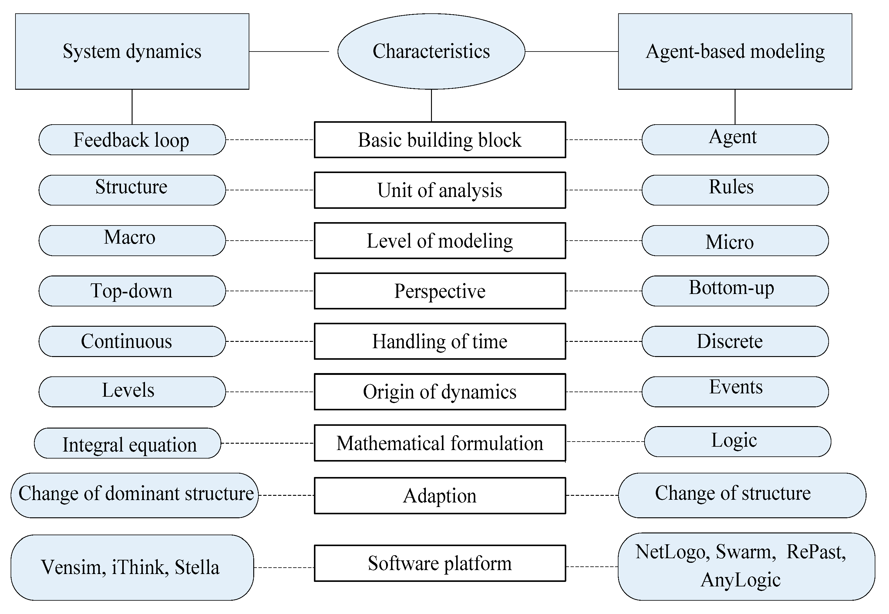
Figure 2.
Definition of neighbourhood for a farmer.
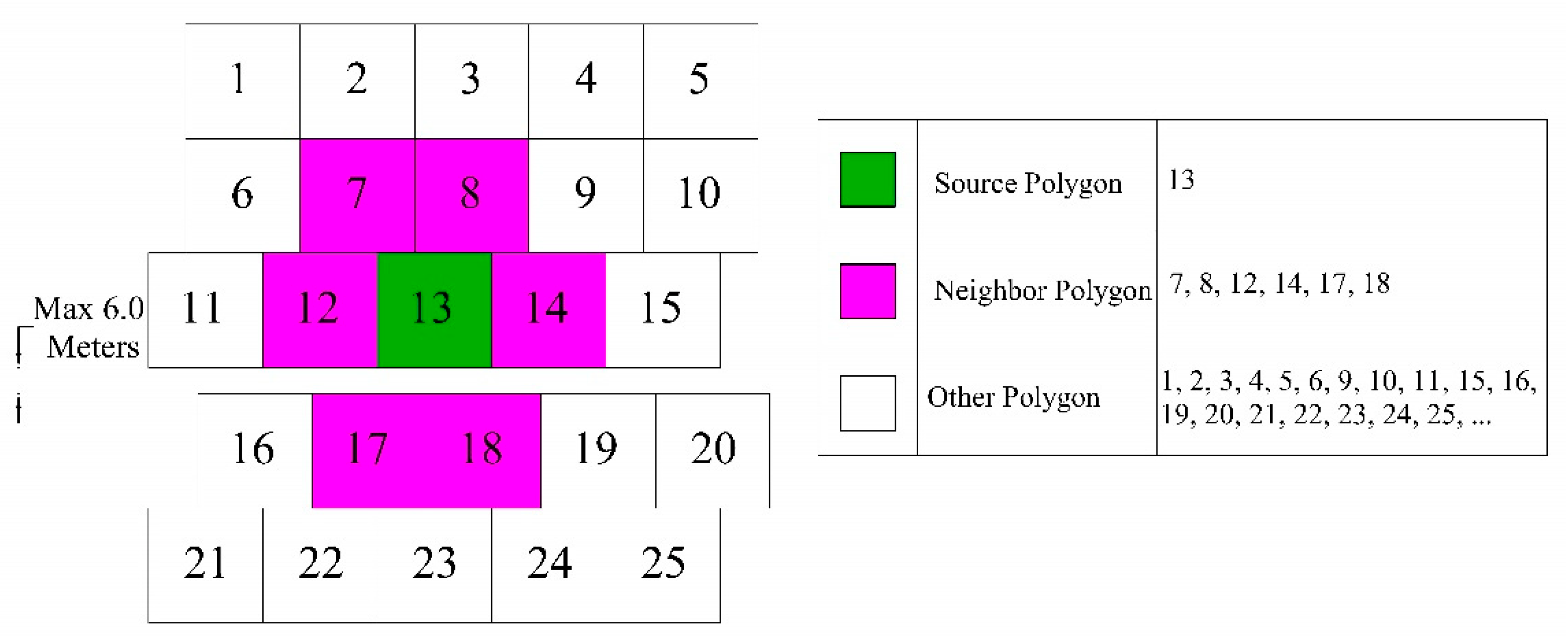
Figure 3.
The Proposed ABM Flowchart.
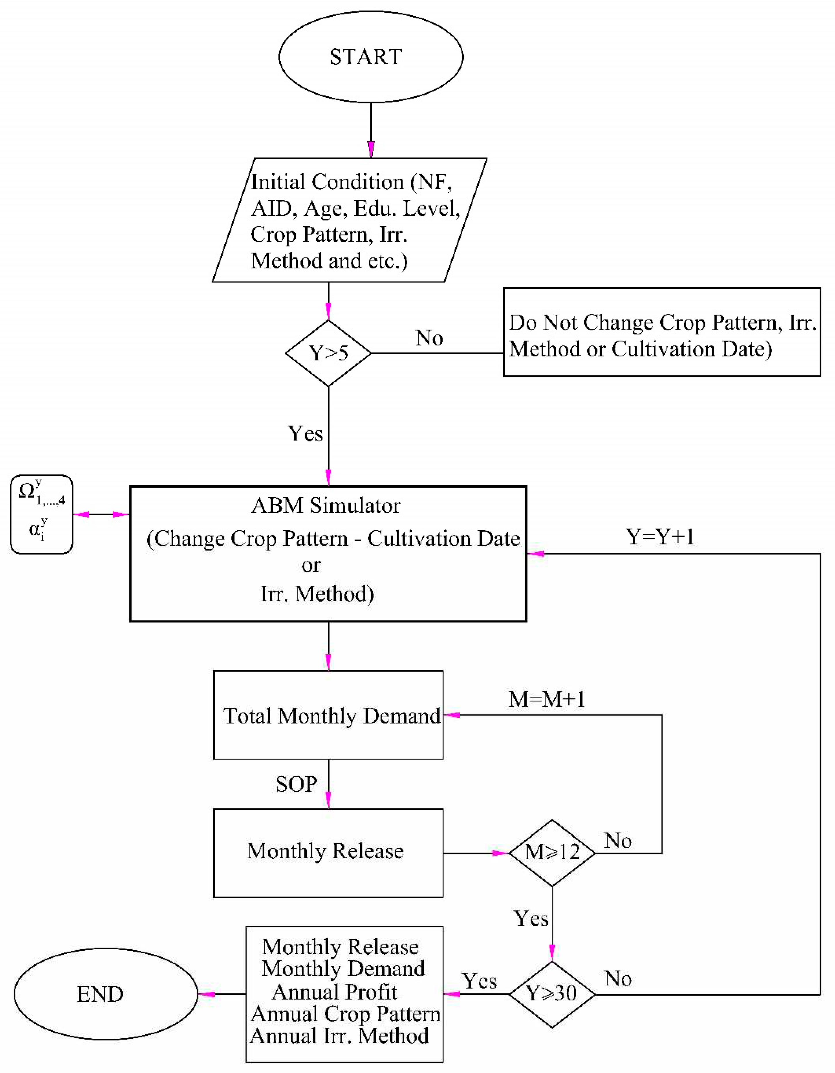
Figure 4.
Initial agricultural lands site plan.
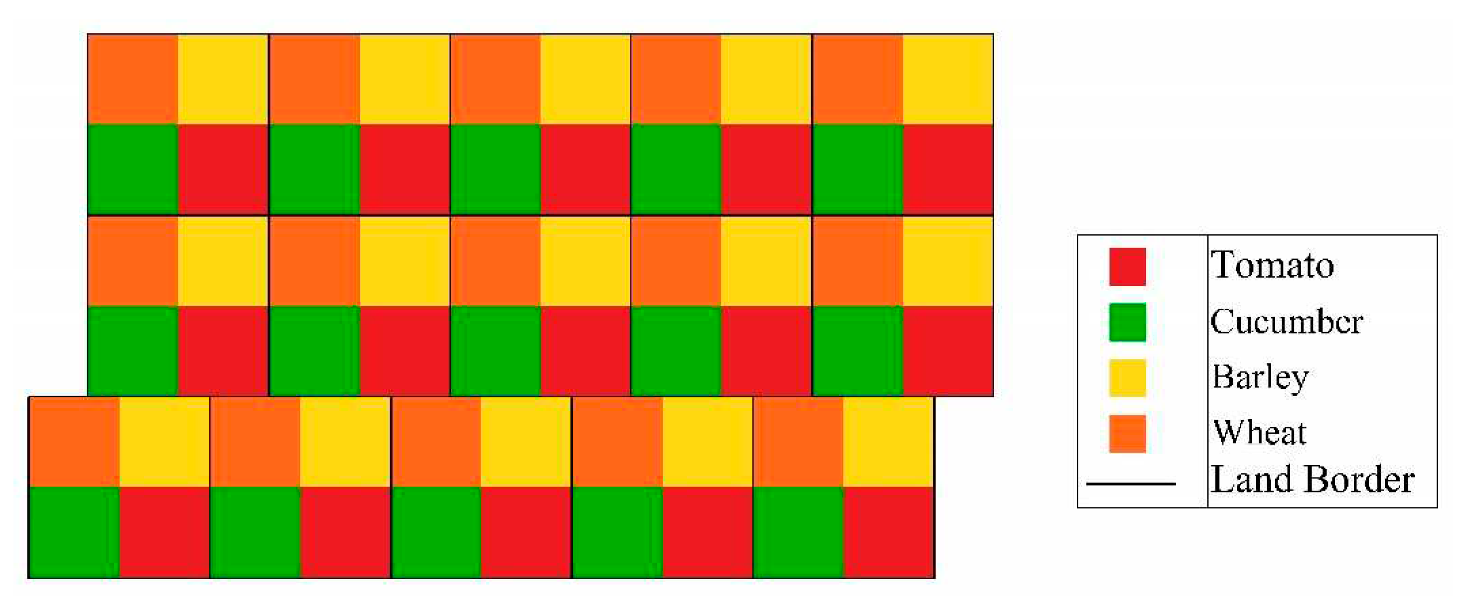
Figure 5.
Agricultural demand fluctuations in ABM1 Scenario.
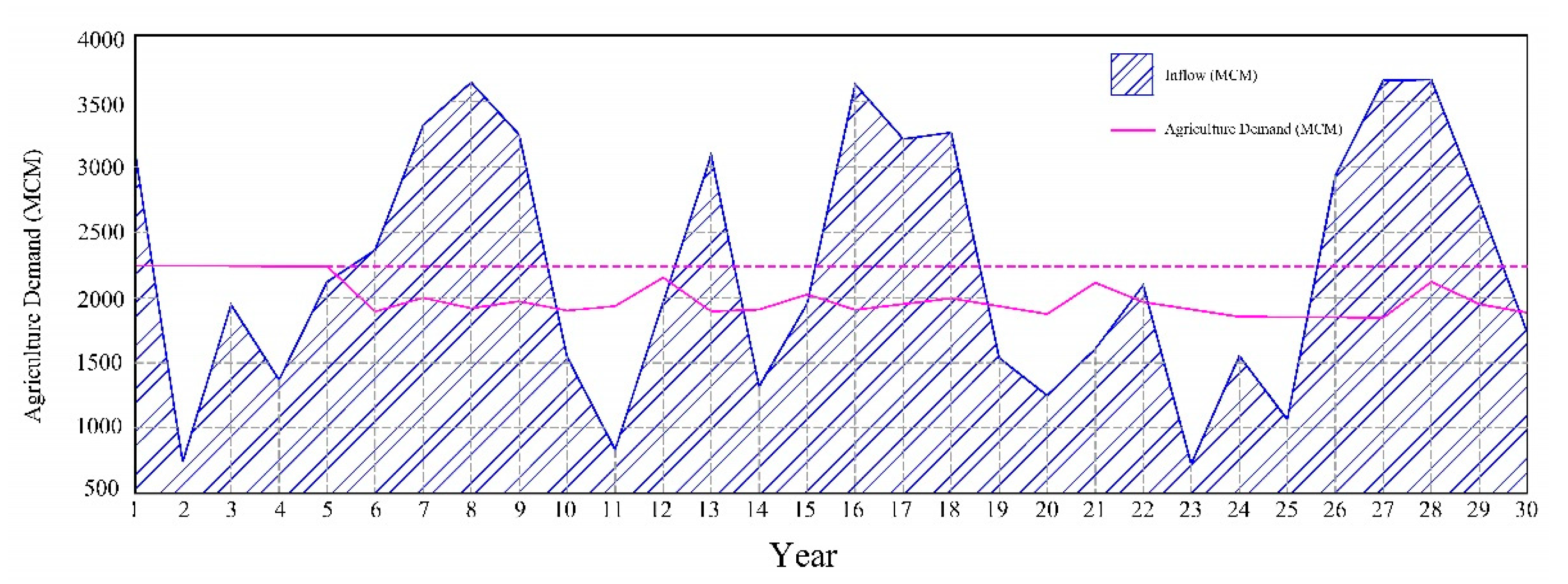
Figure 6.
Deficit fluctuations in ABM1 Scenario and constant agriculture demand case.
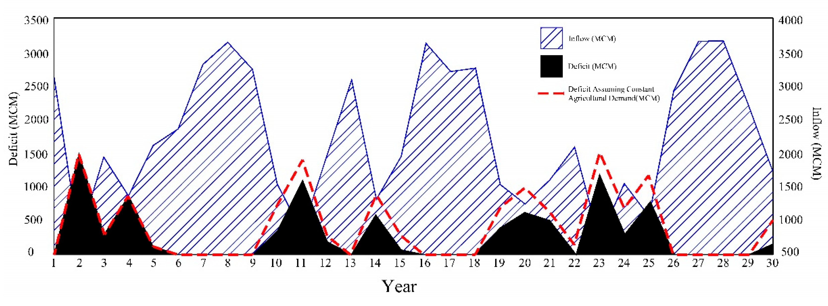
Figure 7.
Profit fluctuations in ABM1 Scenario and constant agriculture demand case.
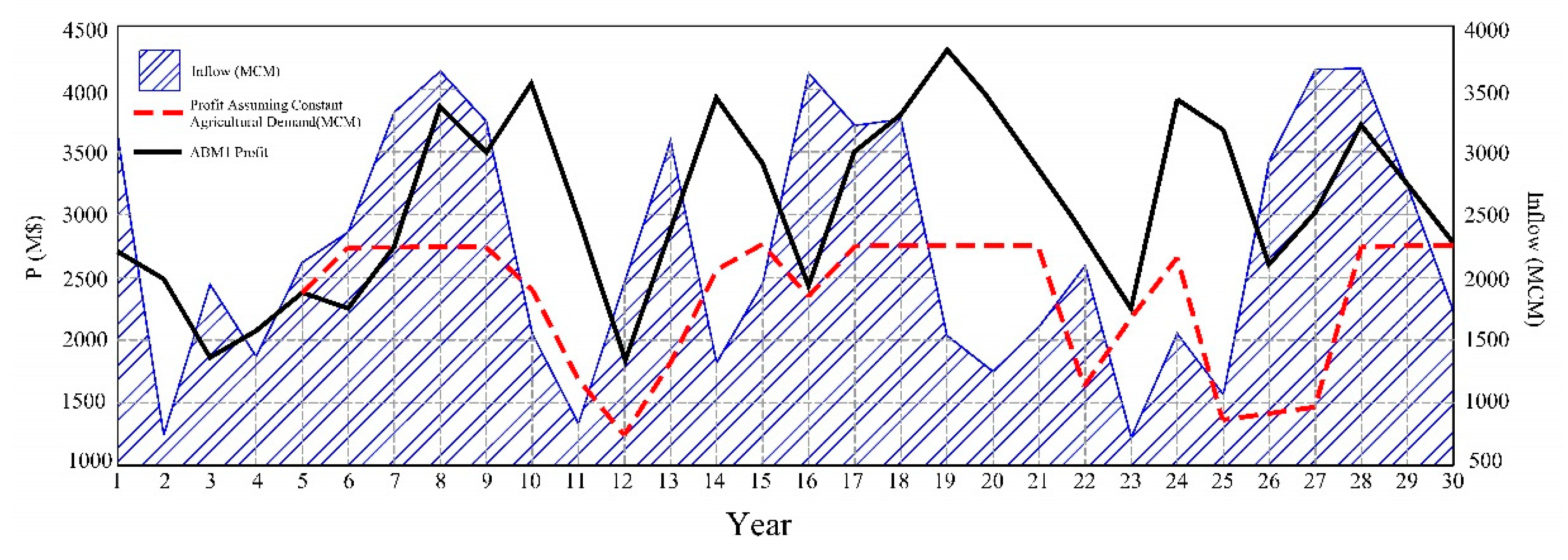
Figure 8.
Farmers’ profit diagram in terms of α (level of risk-taking of farmers).
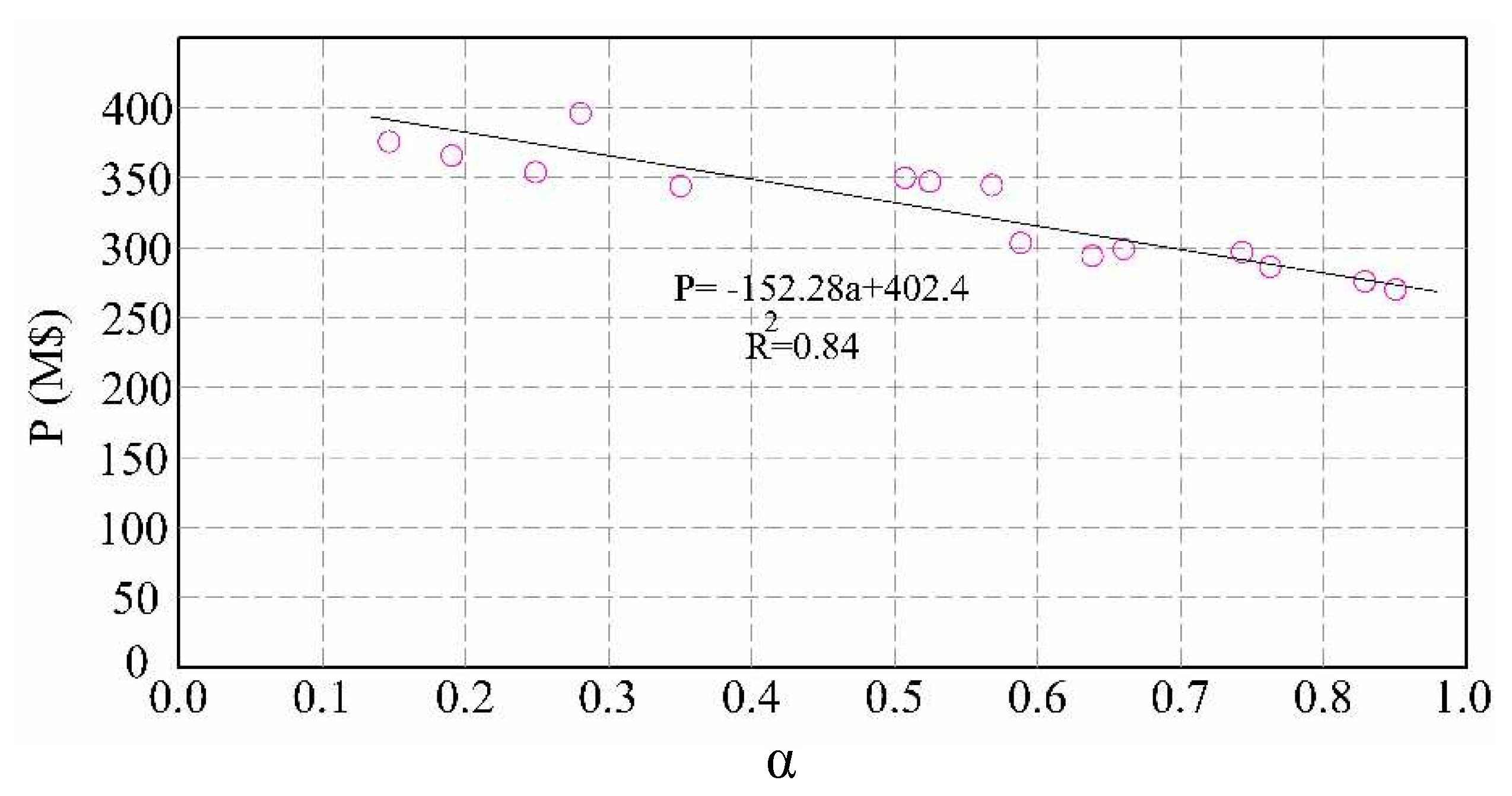
Figure 9.
Agricultural demand band in ABM2 Scenario.
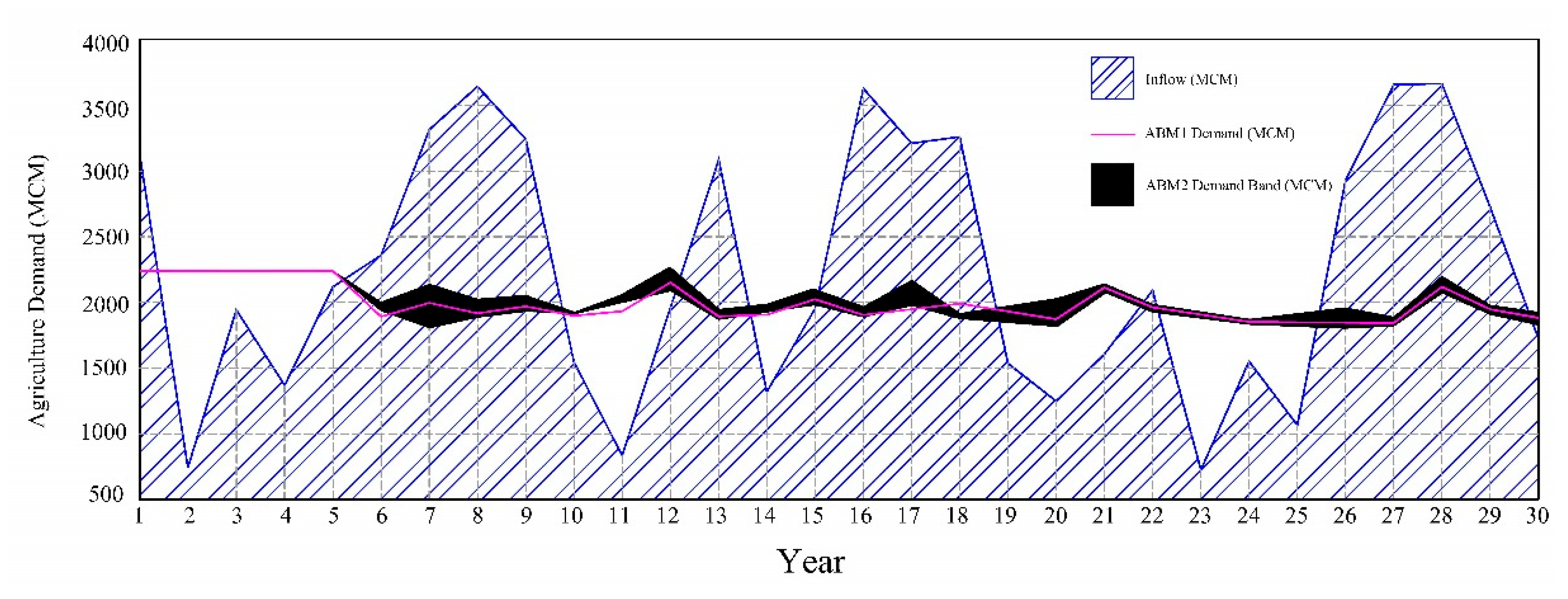
Figure 10.
Matrix of profit (M$) based on α parameter.
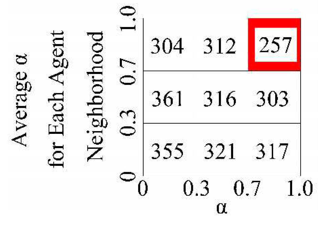

Table 1.
Thresholds for obtaining knowledge about new irrigation technology.
| High Educated Farmer | δ1 | δ2 | δ3 | δ4 |
| Low Educated Farmer | δ5 | δ6 | δ7 | δ8 |
Table 2.
Decide for using new irrigation technology.
| High Educated Farmer | - | 0 | + | + |
| Low Educated Farmer | - | - | 0 | + |
Table 3.
Characteristics of the farmers.
| Farmer ID | Age | AID (%) | Edu. Level | α |
| 1 | 24 | 15 | H | 0.85 |
| 2 | 36 | 35 | H | 0.64 |
| 3 | 55 | 85 | L | 0.15 |
| 4 | 60 | 45 | L | 0.51 |
| 5 | 18 | 55 | L | 0.57 |
| 6 | 45 | 45 | H | 0.53 |
| 7 | 30 | 35 | L | 0.66 |
| 8 | 20 | 30 | H | 0.74 |
| 9 | 19 | 20 | L | 0.83 |
| 10 | 42 | 80 | L | 0.25 |
| 11 | 38 | 40 | H | 0.59 |
| 12 | 25 | 25 | L | 0.76 |
| 13 | 55 | 70 | L | 0.28 |
| 14 | 45 | 65 | H | 0.35 |
| 15 | 55 | 80 | L | 0.19 |
Disclaimer/Publisher’s Note: The statements, opinions and data contained in all publications are solely those of the individual author(s) and contributor(s) and not of MDPI and/or the editor(s). MDPI and/or the editor(s) disclaim responsibility for any injury to people or property resulting from any ideas, methods, instructions or products referred to in the content. |
© 2023 by the authors. Licensee MDPI, Basel, Switzerland. This article is an open access article distributed under the terms and conditions of the Creative Commons Attribution (CC BY) license (http://creativecommons.org/licenses/by/4.0/).
Copyright: This open access article is published under a Creative Commons CC BY 4.0 license, which permit the free download, distribution, and reuse, provided that the author and preprint are cited in any reuse.


