Extraction of Significant Features by Fixed-Weight Layer of Processing Elements for the Development of an Effective Spiking Neural Network Classifier

In this paper, we demonstrate that fixed-weight layers, generated from random distribution or logistic functions, can effectively extract significant features from input data, resulting in high accuracy on a variety of tasks, including Fisher’s iris, Wisconsin Breast Cancer, and MNIST datasets. We have observed that logistic functions yield high accuracy with less dispersion in results. We have also assessed the precision of our approach under conditions of minimizing spikes number generated in the network, it is a practically useful for reducing energy consumption in spiking neural networks. Our findings reveal that the proposed method demonstrates a highest accuracy on Fisher’s iris and MNIST datasets with logistic regression. Furthermore, they surpass the accuracy of the conventional (non-spiking) approach using logistic regression in the case of Wisconsin Breast Cancer. We have also investigated the impact of non-stochastic spike generation on accuracy.

Keywords:

Subject: Computer Science and Mathematics - Artificial Intelligence and Machine Learning

1. Introduction

Spiking neural networks (SNNs), considered as the third generation of artificial neural networks, combine inspiration from biological neural networks with the capability to address traditional machine learning tasks. In SNNs, neurons are dynamic systems that communicate through current impulses.

Over the past two decades, alongside the rapid development of spiking neural networks, neuromorphic processors have emerged, such as TrueNorth [1], Loihi [2], Tianjic [3], and others [4]. These processors realize models which imitate functionality existing in the nervous system and perform machine learning, including realizations of reservoir-based spiking neural network topologies rooted on short-term effects [5] and long-term effects [6]. Their primary advantages include low energy consumption as demonstrated for ZnO-based memristor [7], high parallelism as demonstrated for image skeletonizing [8], signal processing efficiency as shown in [9] for a device with a very low switching current level and self-rectifying characteristics that can be utilized for reservoir computing and real-time adaptability as was discussed in [10]. Efficient solutions for a set of tasks, such as sensory information processing as demonstrated for novel artificial retinal neuron with ultra-low power in [11], pattern analysis as for Fashion MNIST dataset [12], speech recognition, e.g. for the Texas Instruments digit sequences dataset in [13] and the Free Spoken Digits dataset [14], and other perception and environment interaction-related activities as for reinforcement learning in [15] can be achieved by neuromorphic processors. In some cases, this requires the application of methods based on the utilization of a limited number of trainable synaptic weights, which necessitates the development of spiking neural network topologies with limited plasticity synapses [16]. This concern is especially pertinent when training networks on a chip. Lowering the number of trainable weights offers advantages such as reduced overfitting [17], simplifying the fitting algorithm’s complexity, and thus facilitating implementation on neuromorphic processors.

Our approach involves utilizing spiking networks with fixed synaptic weights that remain unchanged during training. This reduces the number of tunable network parameters, simplifying the potential hardware implementation of training on neuromorphic computing devices. This approach is inspired by reservoir neural networks [18]. However, instead of a reservoir with recurrent connections, we use a fully-connected layer with weights fixed based on logistic functions or a uniform random distribution. This approach has been previously demonstrated for conventional neural networks [19] and subsequently extended to spiking networks [20,21]. In our work, we explore the capabilities of layers with fixed weights in solving benchmark tasks of real-valued vector and image classification. With this aim, the current paper presents the following contributions:

We demonstrate the ability of the proposed layer to perform effective reduction in the dimension of the input data vectors without loss of classification performance;
We explore the tradeoff between the number of spikes needed for encoding the input information and classification performance, so that to find input encoding parameters that minimize the number of spikes while maintaining competitive classification performance;
We compare different methods for initializing the weights of the proposed layer.

As the result, we find that:

Layers with random or logistic function-generated weights can efficiently extract meaningful features from input data;
Logistic functions enable achieving high accuracy with less result dispersion.

We conduct numerical experiments on a set of commonly-used benchmark datasets described in Section 2: Fisher’s Iris, Wisconsin Breast Cancer, and MNIST. The spiking network used is described in Section 3. Section 4 provides descriptions of the experiments and their results. Finally, an analysis of the results is presented in Section 5.

2. Datasets

Several datasets, available in the scikit-learn library for Python, are utilized to evaluate the quality of the proposed approach:

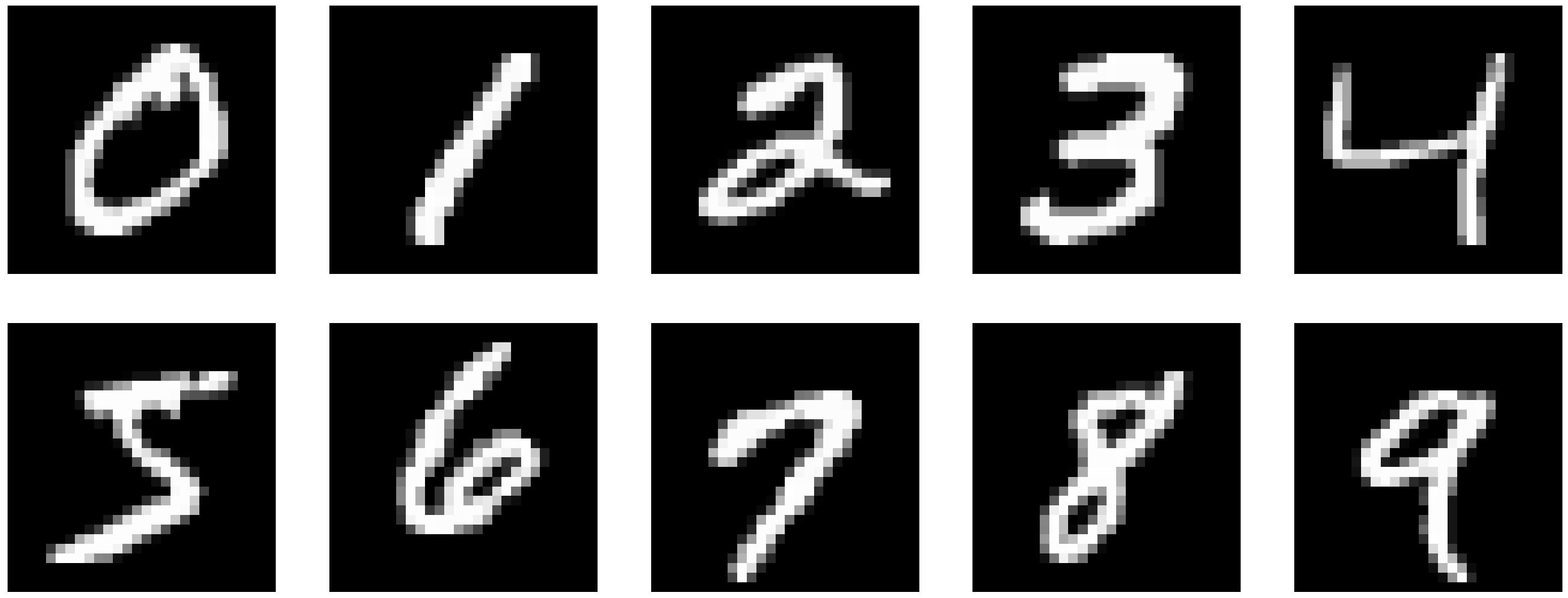
The MNIST dataset contains 60 000 training and 10 000 testing black-and-white images of size 28x28 pixels, representing handwritten digits from 0 to 9. The brightness of each pixel ranges from 0 to 255, where 0 corresponds to an absolutely black pixel and 255 to an absolutely white pixel. This dataset has become a benchmark for evaluating the performance of various classification algorithms. The examples from the dataset are depicted in Figure 1.
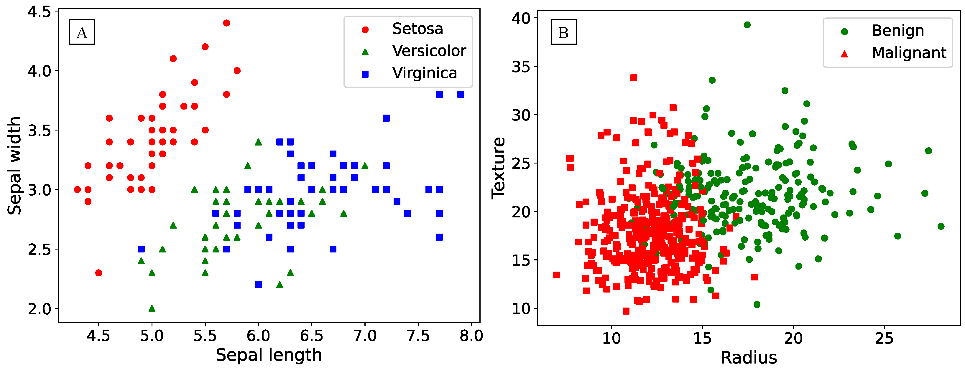
The Fisher’s Iris dataset contains 150 samples of iris flowers, with 50 samples for each of the three species. Each sample consists of four numeric features describing the length and width of the sepals, and the length and width of the petals. The data visualization is presented in the Figure 2 A, illustrating the non-linearity of the task using only two features.
The Breast Cancer Wisconsin (Diagnostic) dataset consists of 569 samples, containing information on cell characteristics from breast biopsy samples and their corresponding diagnosis: malignant or benign tumor, with 212 and 357 samples respectively. The features are numeric and describe the morphological and structural characteristics of the cells, such as nucleus size, radius, area, and others. The data visualization, as shown in Figure 2 B, employs only two features, akin to the case of Fisher’s irises.

3. Spiking neural network

3.1. General architecture

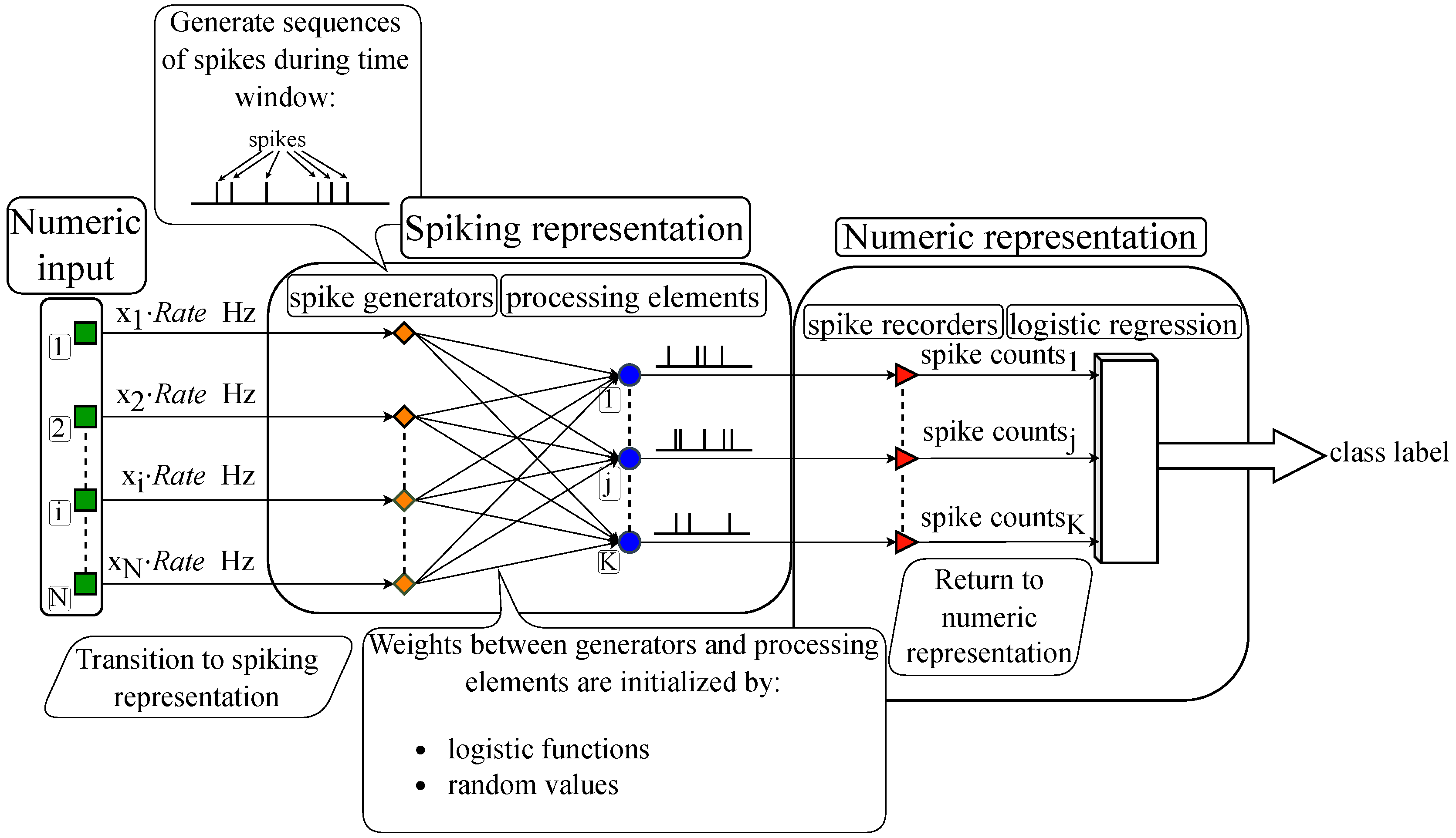
Figure 3 illustrates the proposed algorithm’s general scheme: The input is encoded from numeric representation into spike sequences, which are fed into the spiking layer, then the output spike sequences emitted by the layer are subsequently decoded back into numeric representation and processed by the classifier.

3.2. Spike generators

The transition from numeric to spiking representation of the input is based on frequency encoding, where a higher input value (e. g. for digit images, higher brightness) means higher number of spikes emitted by the corresponding generator in the spiking neural network. The advantage of frequency encoding lies in its naturalness and biological analogy, as neurons in the brain, for instance, in sensory cortical areas, often respond to signals by changing the spike generation frequency.

This numeric-to-spiking transition of performed by a layer of N spike generators, where N is the input dimension. The output of each generator is a sequence of spikes, the times of these spikes aligned to numerical simulation timesteps of 0.1 ms. Poisson generators emit spikes at random times so that the total number of spikes in the sequence that encodes its corresponding input vector component

x_{i}

obeys a Poisson distribution with the mean

x_{i} \cdot Rate

. Poisson generators, further referred to as stochastic generators, are used in all experiments except SubSection 4.6, where they are compared to non-stochastic generators that emit spikes with equal interspike intervals, keeping the total number of spikes equal to

x_{i} \cdot Rate

. Here,

R a t e

is an adjustable coefficient which is examined during the experiments.

3.3. Processing elements

We consider two types of processing elements. The first one is the Leaky Integrate-and-Fire spiking neuron with exponential post-synaptic currents. The dynamic of this neuron model is described by the following system:

\{\begin{matrix} \frac{d V_{j}}{d t} = - \frac{V_{j} - V_{rest}}{τ} + \frac{I_{j}^{syn}}{C}, \\ I_{j}^{syn} = \sum_{i} (w_{i j} \cdot I * \sum_{t_{i j}^{spike}} δ (t_{i j}^{spike})), \\ I (t) = e^{- \frac{t}{τ_{syn}}}, \\ V_{m} \geq V_{th} \Rightarrow V_{m} = V_{rest}, \end{matrix}

(1)

where

V_{j}

is the membrane potential of j-th neuron,

V_{rest} =

-70 mV is the resting potential,

τ =

10 ms is the synaptic decay time constant,

I_{syn}

is the total synaptic current,

C =

250 pF is the membrane capacitance,

w_{i j}

is the synaptic weight,

I_{i j}

is the individual synaptic current,

t_{spike}

is spike timing, and

τ_{syn} =

2 ms is the time constant of synaptic current. The asterisk (*) denotes convolution, and the sum is over the input synapses i of neuron j, and then over all times

t_{i j}^{spike}

of input spikes arriving at the i-th input of neuron j When the neuronal membrane potential reaches a threshold value of

V_{th}

, the neuron fires a spike, and the membrane potential resets to the

V_{rest}

value and remains unchanged during

t_{ref} =

2 ms.

V_{th}

was adjusted during the experiments.

After presenting an input vector to the spiking layer, the output of the spiking neuron is the number of spikes it emits.

In order to assess separately the influence of the discrete nature of the output of a spiking neuron, we also use another type of processing element, further referred to as Adder. It is an element that receives a vector of numbers of spikes emitted by spike generators as an input

s p i k e_c o u n t s_{i}

, then multiplies it by a vector of weights

w_{i j}

corresponding to this element j, and outputs the result:

o u t_{j} = \sum_{i = 1}^{N} w_{i j} \cdot s p i k e_c o u n t s_{i} .

(2)

Effectively, the output of an adder is the upper limit of the output a spiking neuron with infinitely small threshold and simulation timestep. On the plots, the adder is therefore symbolically placed as if it had

V_{th} = V_{rest}

3.4. Weight initialization

Below, we use and further compare two methods of weight initialization:

Random values — the weights are generated from a uniform distribution within the range of -1 to 1;
Logistic functions — the weights are determined by the values of logistic functions, the general form of which looks as follows:

$\{\begin{matrix} w_{i, 1} = A \cdot sin (\frac{i}{N} \cdot \frac{π}{B}), \\ w_{i, j} + 1 = 1 - r \cdot w_{i, j}^{2}, \end{matrix}$

(3)

that are described in more detail in study [19] and r was set at 1.885, A is 0.3, B is 5.9 for the purposes of this paper, N is a number of inputs.

3.5. Decoding

During a fixed time window, determined through experiments, generators emit spikes from 0 to the maximum per second depending on the feature value. These spikes reach adders or spiking neurons via the weights, triggering them to emit spikes themselves. The numbers of spikes fired by the neurons or the outputs of adders are recorded. At the end of the time window, these values are passed to a logistic regression, which outputs a class label based on the received numeric vector.

4. Experiments and Results

4.1. Agenda of experiments

In our experiments, we aimed to achieve optimal accuracies on the aforementioned benchmarks while using a limited number of spikes. This problem formulation is of practical interest when developing energy-efficient biomorphic systems.

For the benchmarks, we conducted sequences of experiments to clear:

The criteria for selecting the feed time window;
The accuracy dependence on number of processing elements;
The accuracy dependence on the maximal number of spikes in the case of more effective number of processing elements, defined in experiments of point 1;
The accuracy dependence on the number of output spikes with a given number of neurons with thresholds;
The influence of stochastic of input signal on the accuracy.

The experiments were conducted using both weight initialization methods: Logistic functions and Random values. The dependence of accuracy on the time window, the number of processing elements, and the number of input spikes, has been obtained for adders as processing elements, while the influence if spiking neuron dynamics is assessed separately in Section 4.5.

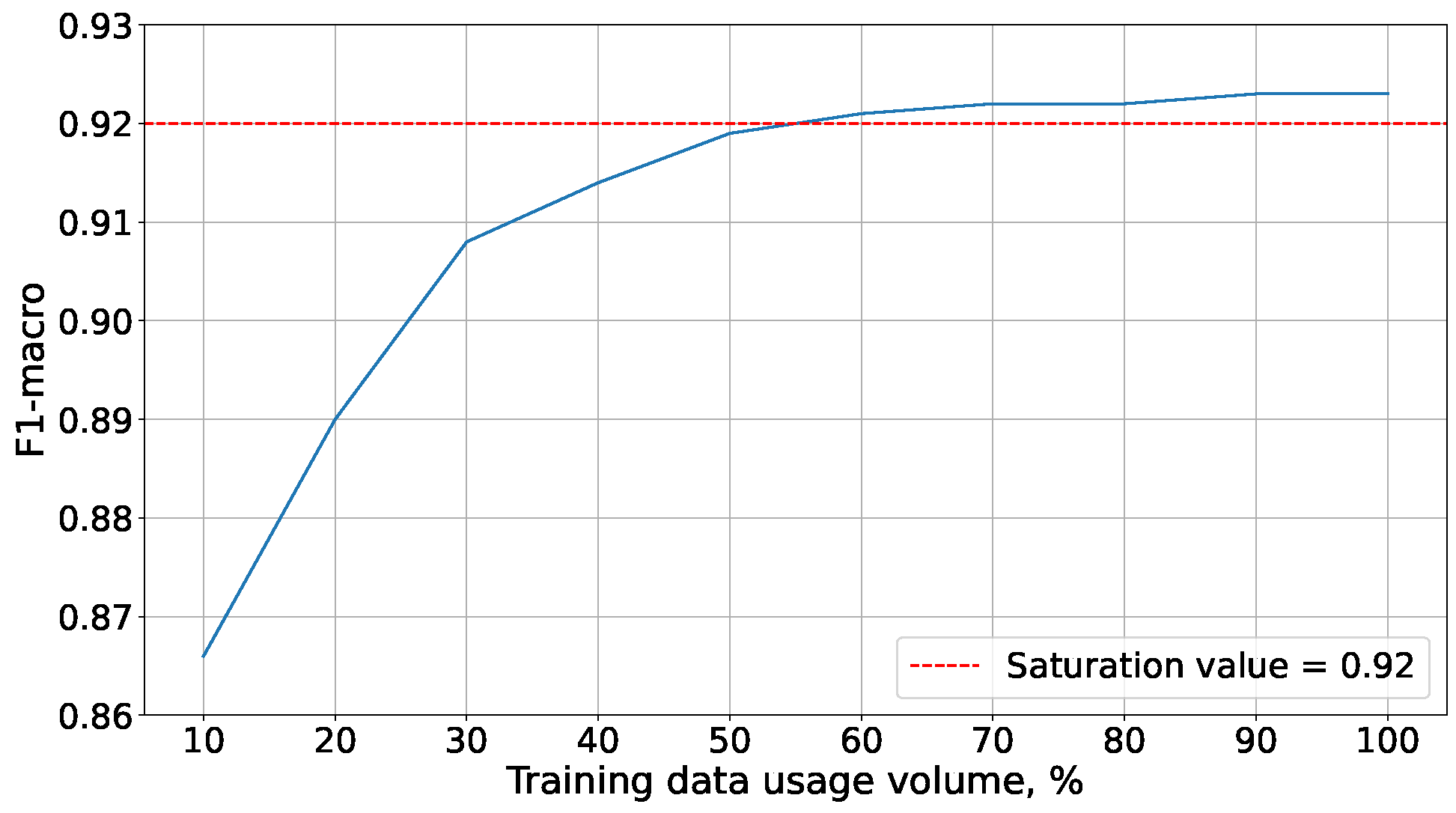
Due to the extensive time required for experiments with MNIST data, they were conducted on a reduced training set. Its size was determined through additional experiments, the results of which are presented in Figure 4. These demonstrated that accuracy saturation on the MNIST dataset is achieved at 60% of the training set. With such a volume of training data, logistic regression reached an accuracy comparable to that obtained on the full training data set:

All subsequent experiments were conducted on the reduced MNIST dataset.

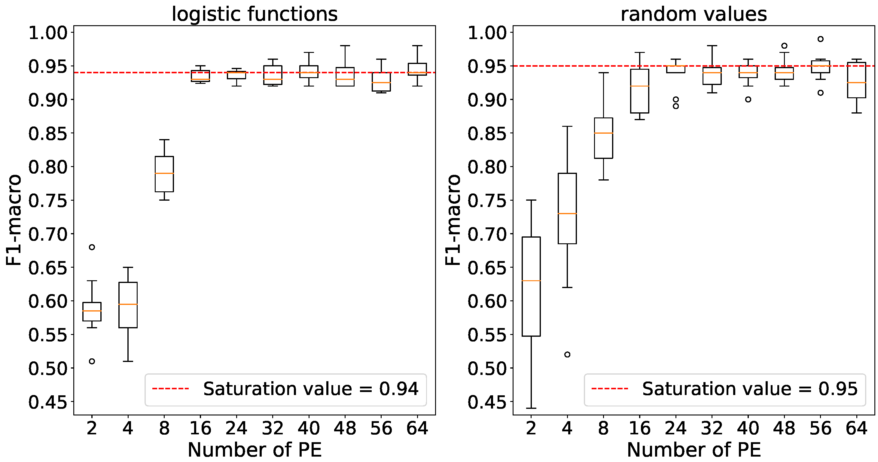
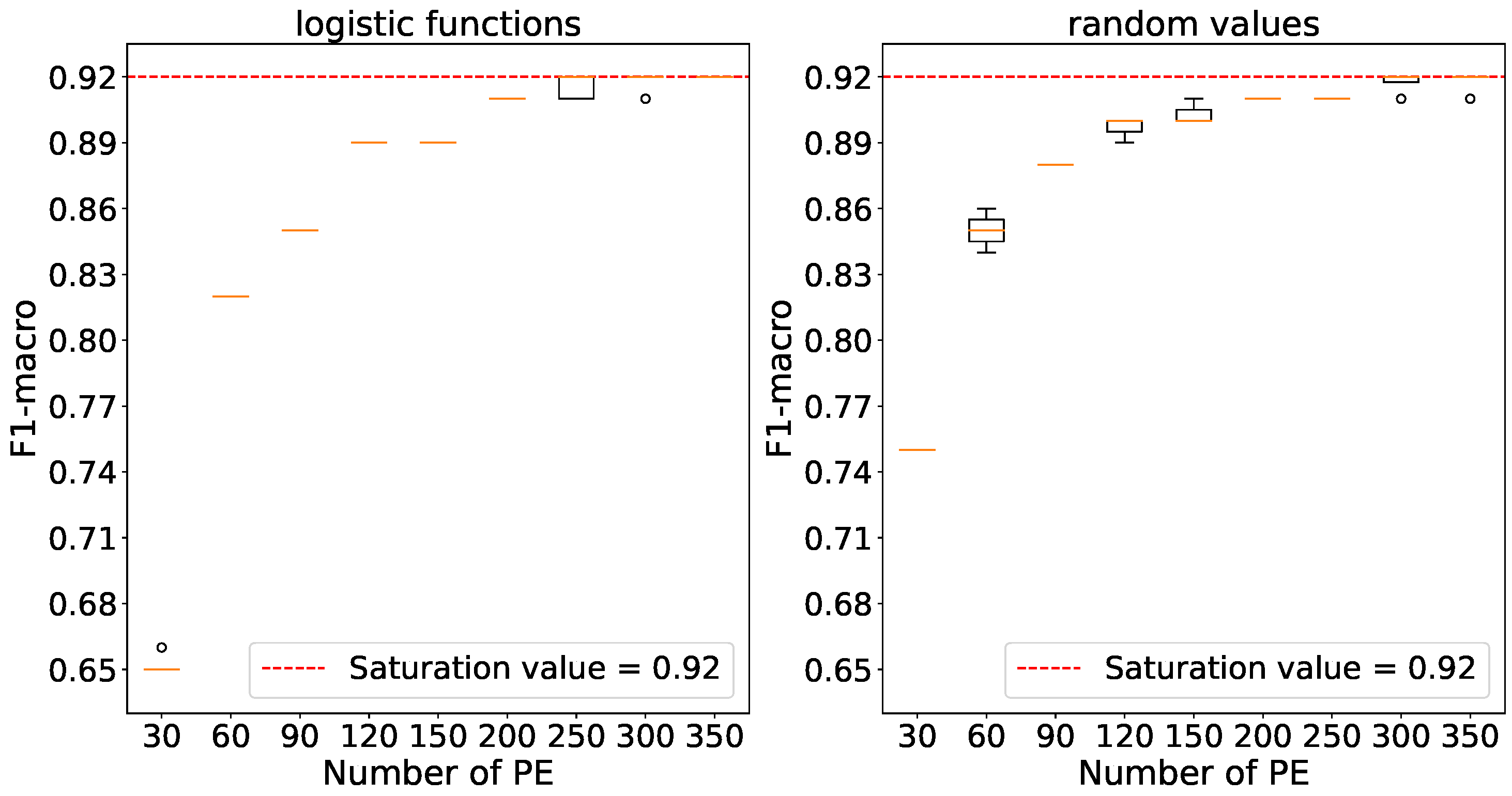
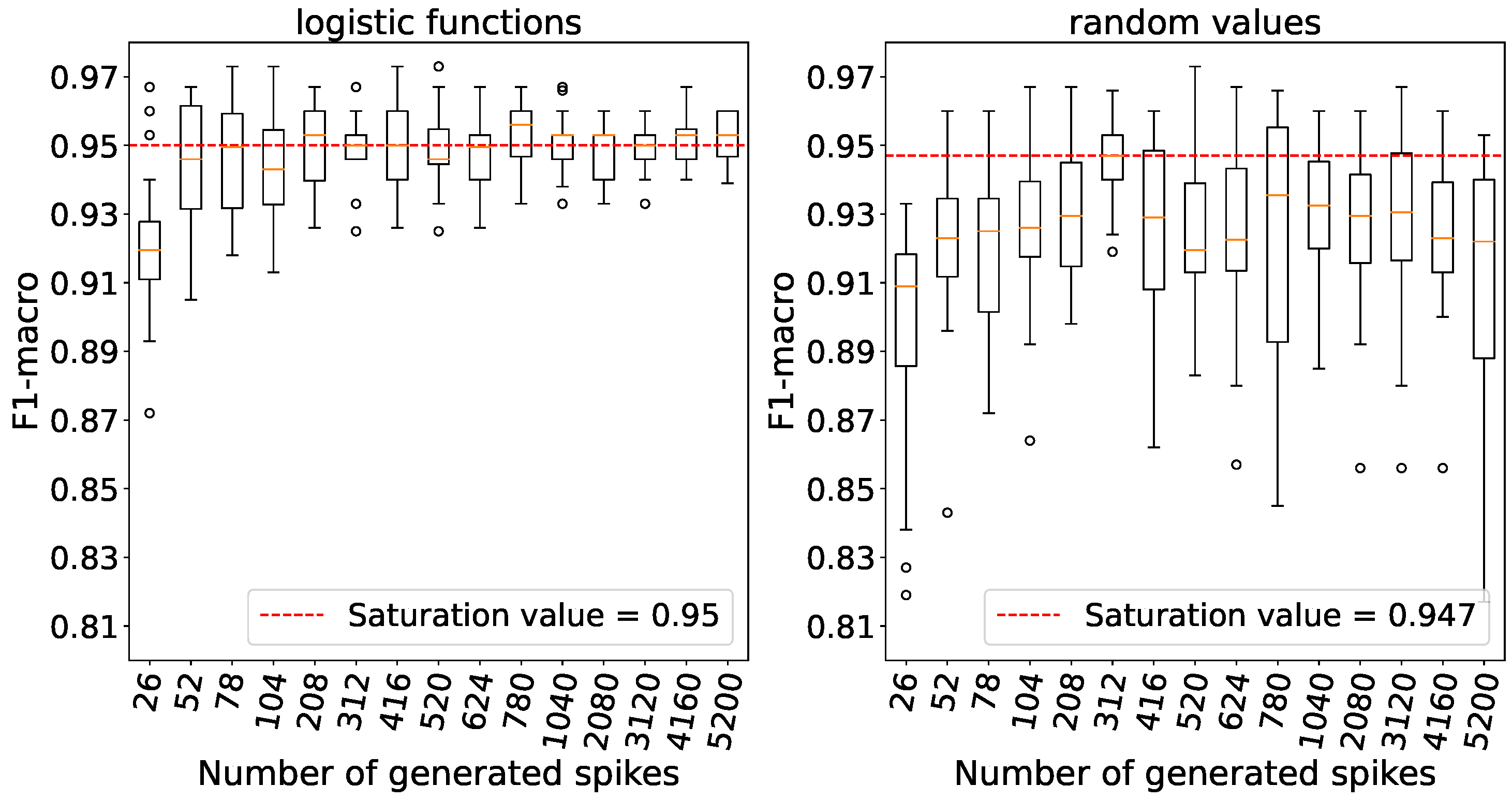
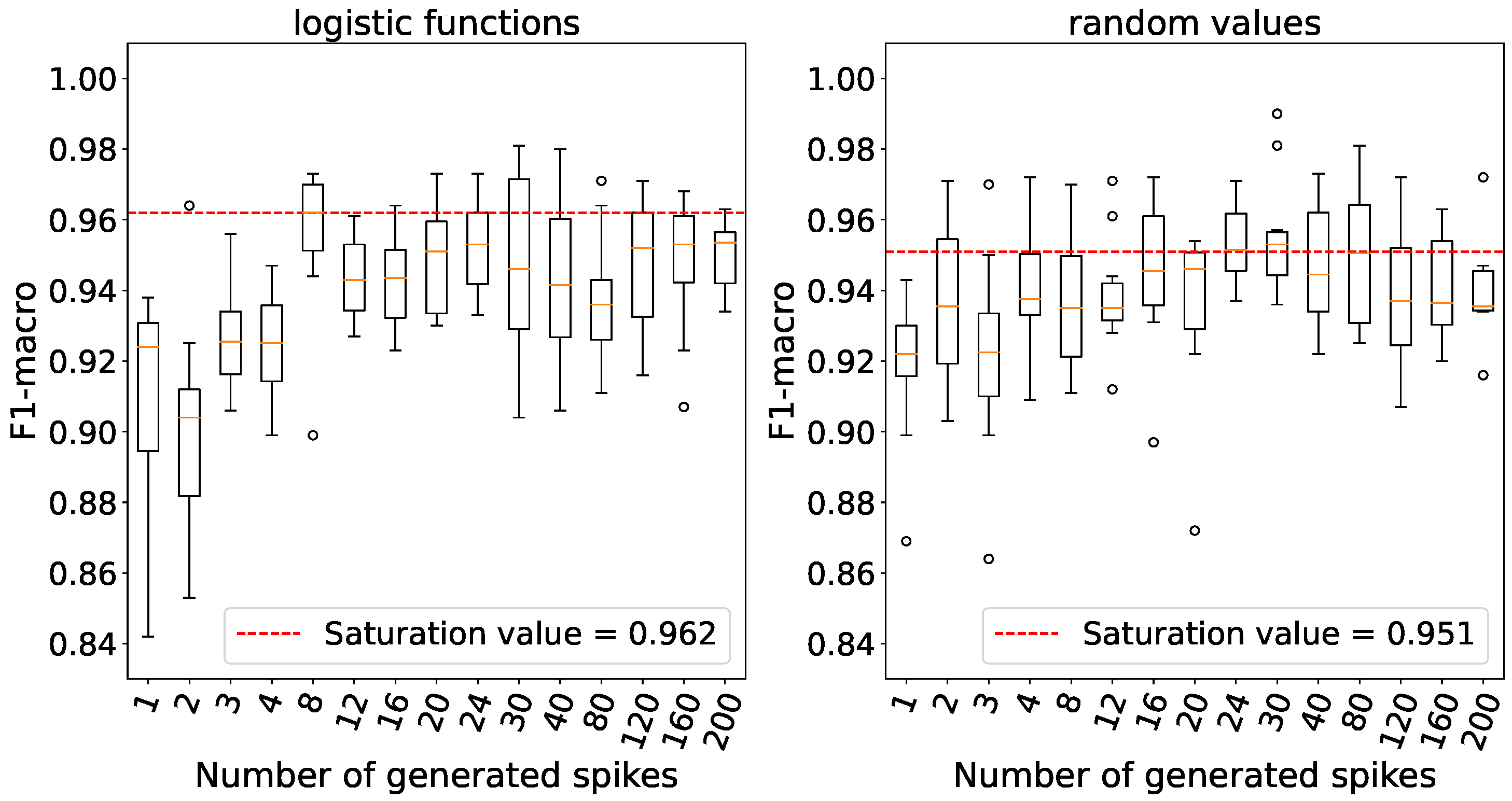
To mitigate the influence of randomness caused by the stochasticity of Poisson spike generators and weight initialization method, we performed several accuracy calculations (further we call it attempt) for each point in the experiments. Additionally, we conducted a 5-fold cross-validation on the Fisher’s Iris and Wisconsin’s Breast Cancer data. The ’box-and-whisker’ plots below are obtained over five attempts for the MNIST dataset and ten attempts for the Fisher’s Iris and Wisconsin’s Cancer datasets. Further in Table 1, the minimum and maximum accuracies obtained across all attempts are presented.

The dotted lines shown on the plots indicate the saturation level of accuracy, determined by the mean values of the boxplots. The parameters with which the saturation level of accuracy was achieved were chosen for subsequent experiments.

4.2. Analyzing the time window size for each dataset

In the experiments conducted in this study, the maximum spike generation frequency of the generators is capped at 1000 Hz. This limitation is imposed to prevent generators from emitting more than one spike per discretization step, which is physiologically implausible. The purpose of this experiment is precisely to determine the minimum temporal window required to achieve optimal accuracy under these constraints.

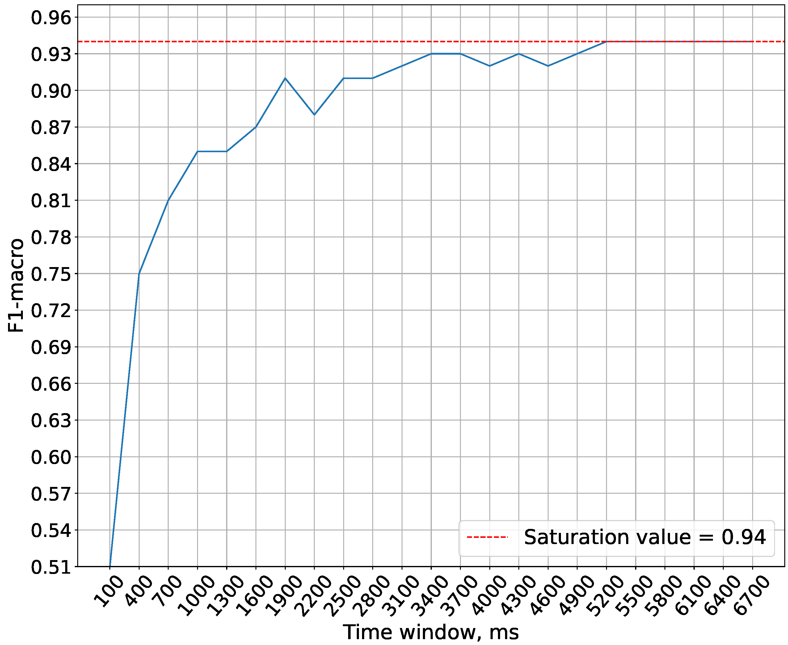
Figure 5 demonstrates that the saturation of accuracy is achieved at a time window size of 5200 ms. Therefore, this time window size is used in future experiments.

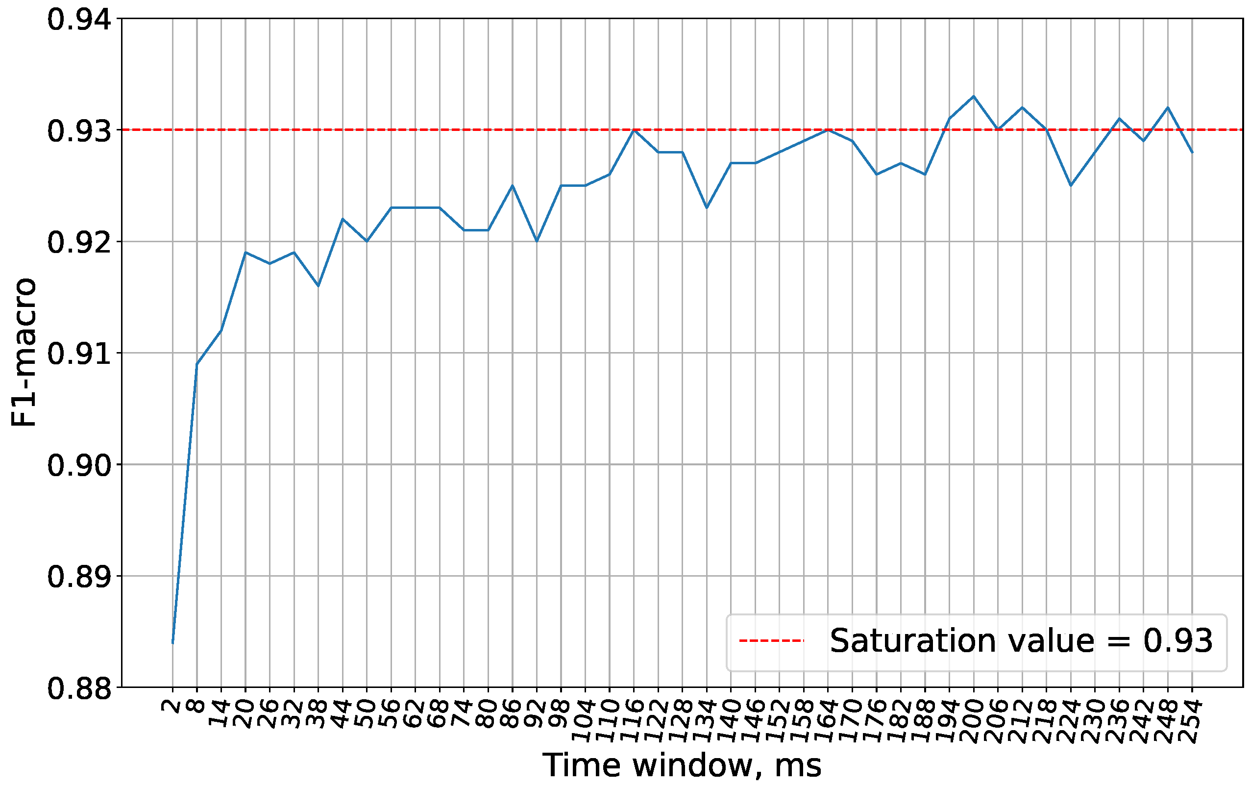
On Figure 6 it is shown that the optimal accuracy with the Wisconsin cancer dataset is achieved with a 200 ms time window. Therefore, this window size is used in subsequent experiments.

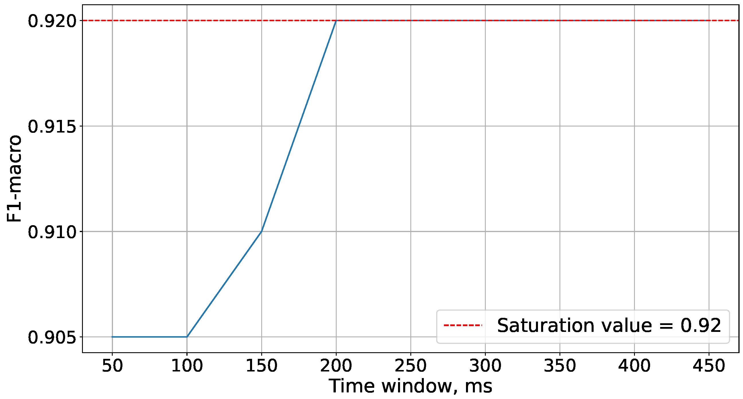
For subsequent experiments, the time window size of 200 ms has been chosen, at which the accuracy saturates as illustrated in Figure 7.

4.3. Searching the optimal number of processing elements

The objective of this experiment was to determine the minimum number of processing elements, directly influencing the amount of spikes propagating through the network, required to achieve saturation accuracy.

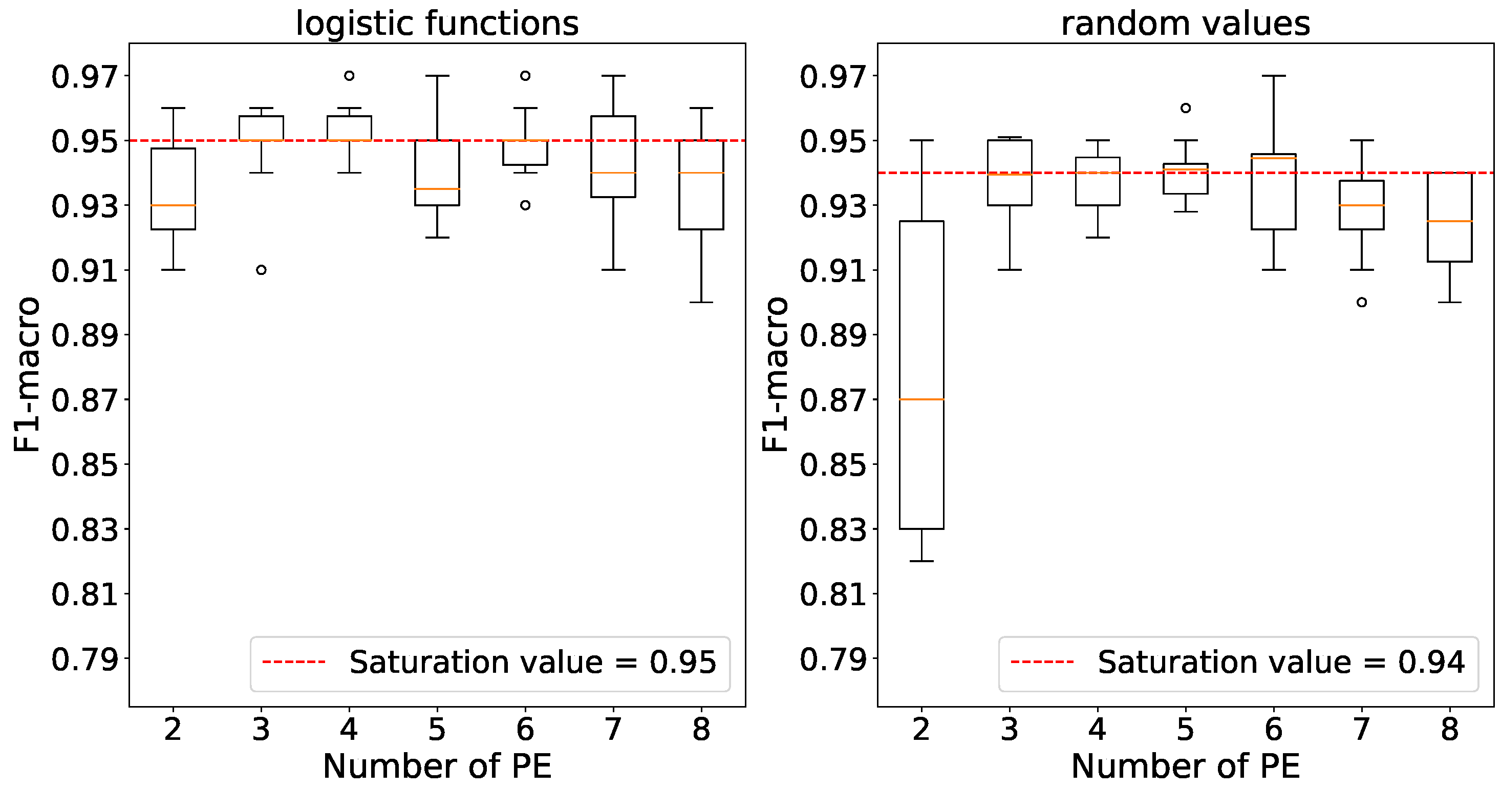
Using 3 processing elements, we observe that accuracy saturates for both weight initializations according to Figure 8.

For the subsequent experiments, we have chosen to use 24 processing elements, as the accuracy plateaus across all initiations at this number of elements following the details in Figure 9.

Figure 10 indicates that maximum accuracies are achieved using 250 processing elements with logistic function initialization and 200 elements with random number initialization. The relevant values have been selected for further experiments.

4.4. Searching the optimal number of generated spikes with a given number of PE from the previous experiments

During this experiment, generator frequencies were gradually increased to establish the minimum number of spikes required to achieve saturation accuracy.

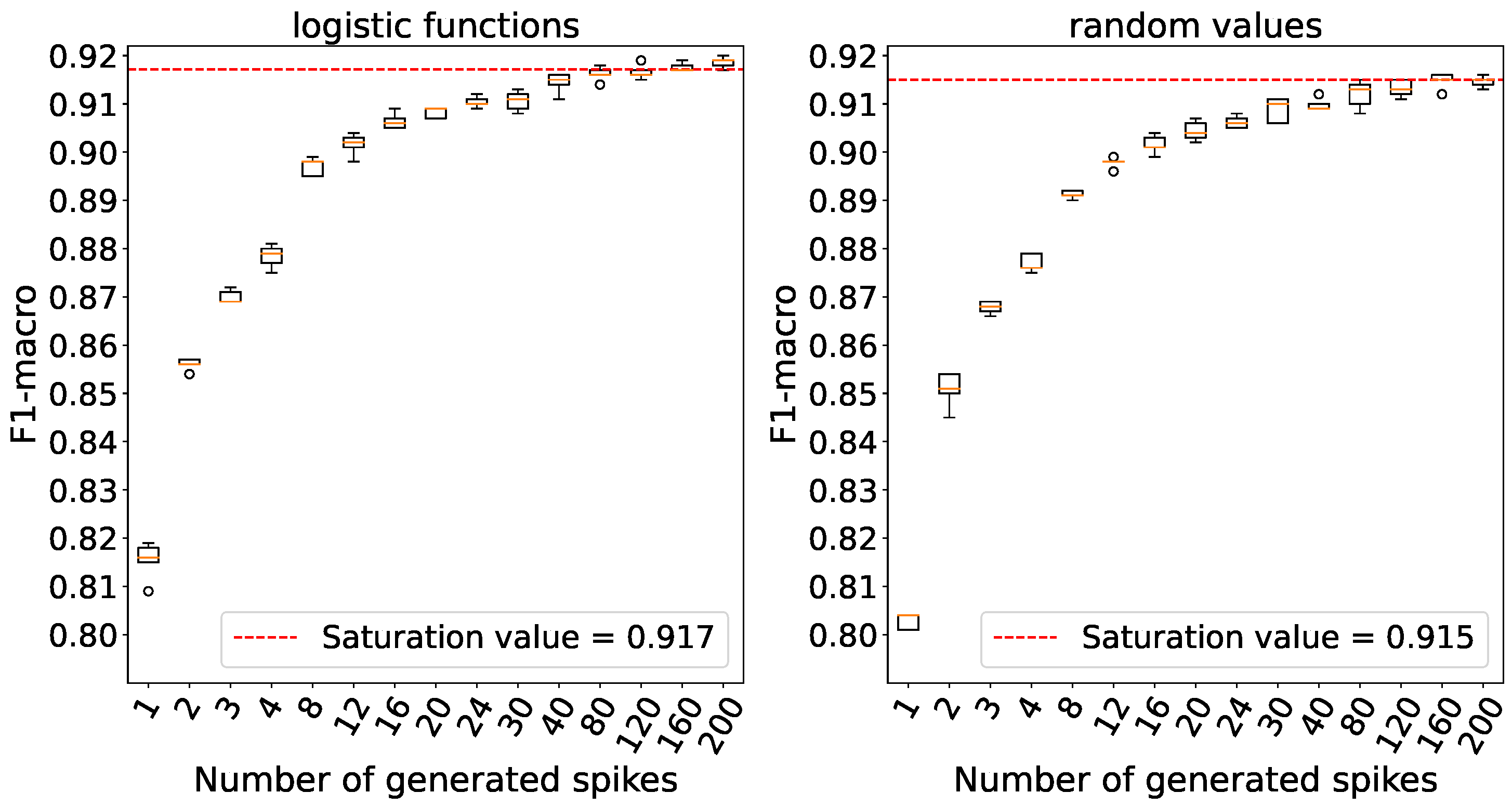
Accuracy reaches saturation with a number of generated spikes set at 52 for logistic weights and 312 for random weights as outlined in Figure 11. For subsequent experiments, we chose a value of 312 for logistic weights because the variance in accuracy is relatively small, and the average accuracy is comparable to that obtained with 52 spikes. It is also worth noting that when weights are initialized with random numbers, the variances in accuracy are higher compared to weight initialization using logistic functions.

Accuracy saturation is achieved with a number of generated spikes set at 8 for logistic weights and 24 for random weights as indicated by the data presented in Figure 12. These respective values were selected for subsequent experiments.

Saturation is reached when the number of generated spikes is set to 160 for both weight initializations as per Figure 13.

4.5. Searching the optimal threshold reflecting the number of output spikes with a given number of processing elements that are replaced by neurons and a number of generated spikes from the previous experiments

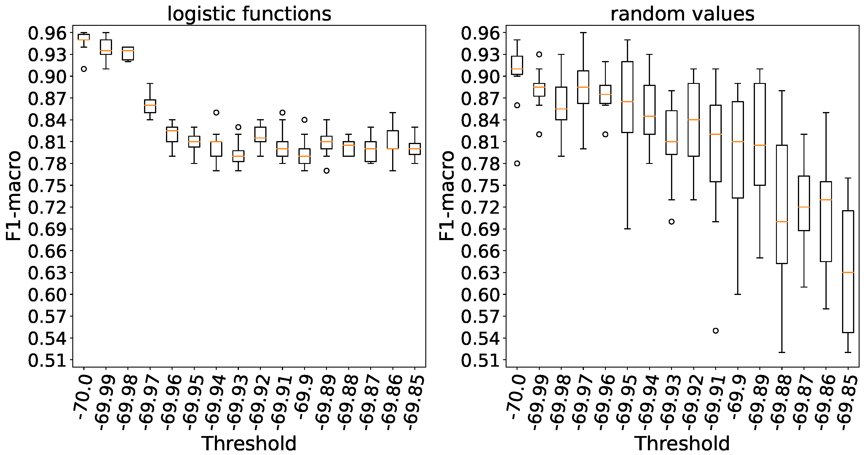
In this experiment, spiking neurons were employed to examine their impact on the accuracy of models. On the graphs, summators are denoted with a conditional threshold of -70.0 mV.

It is important to note that as the threshold potential value increases, the number of emitted spikes decreases. Therefore, the threshold value at which the firing rate saturates is sought from right to left, rather than from left to right as in previous experiments.

Figure 14 clearly demonstrates that processing elements without a threshold yield the highest level of accuracy. Similar to the previous experiment, we observe a relatively significant variance when weights are initialized with random numbers, in contrast to initializing them using logistic functions.

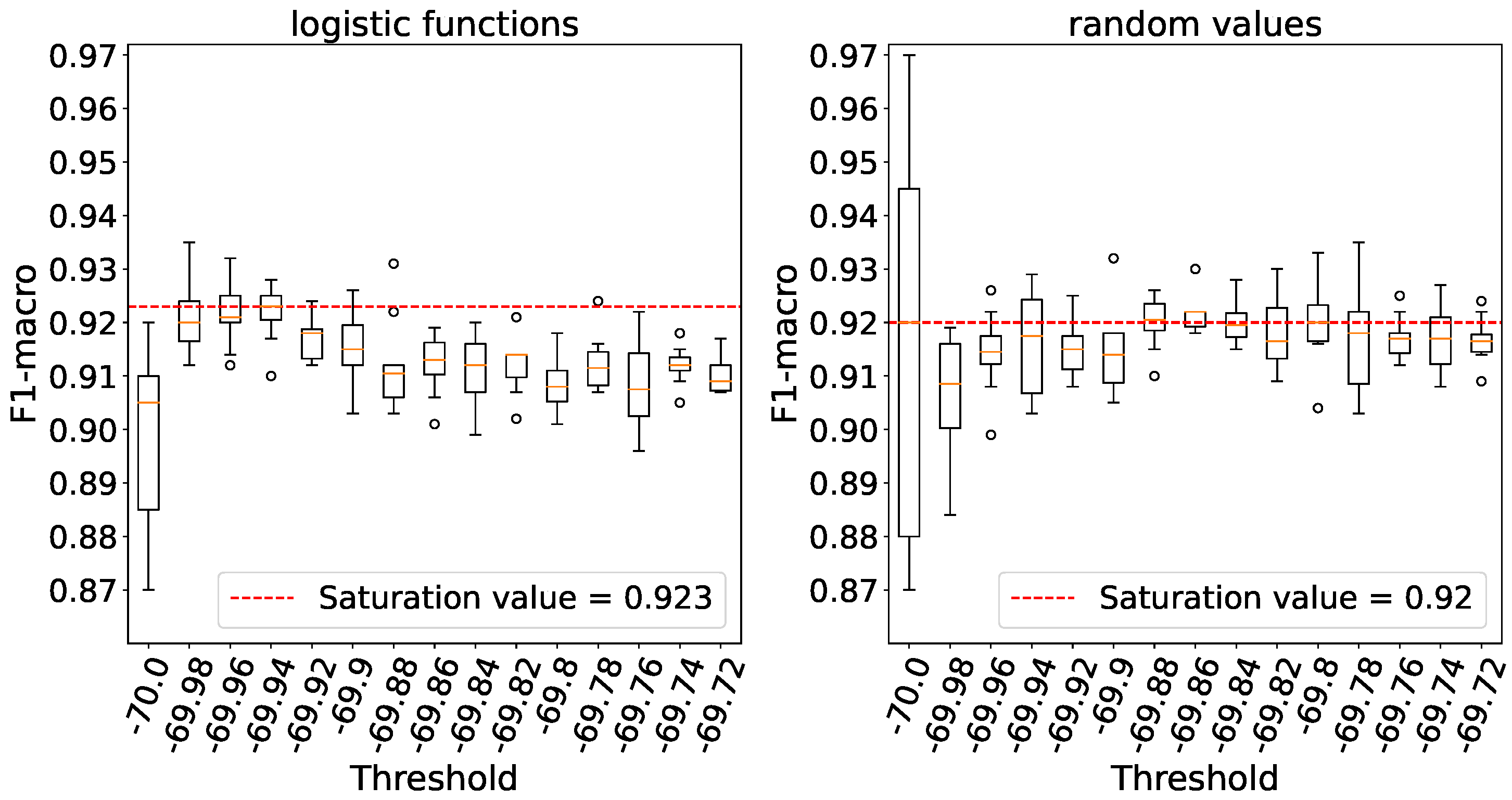
In Figure 15 it is evident that when weights are initialized with logistic functions, accuracy saturates at a threshold of -69.94,whereas with random weights, the plateau accuracy is observed at a threshold of -69.8, taking into account the variance. A higher threshold level indicates a lower number of spikes emitted by neurons.

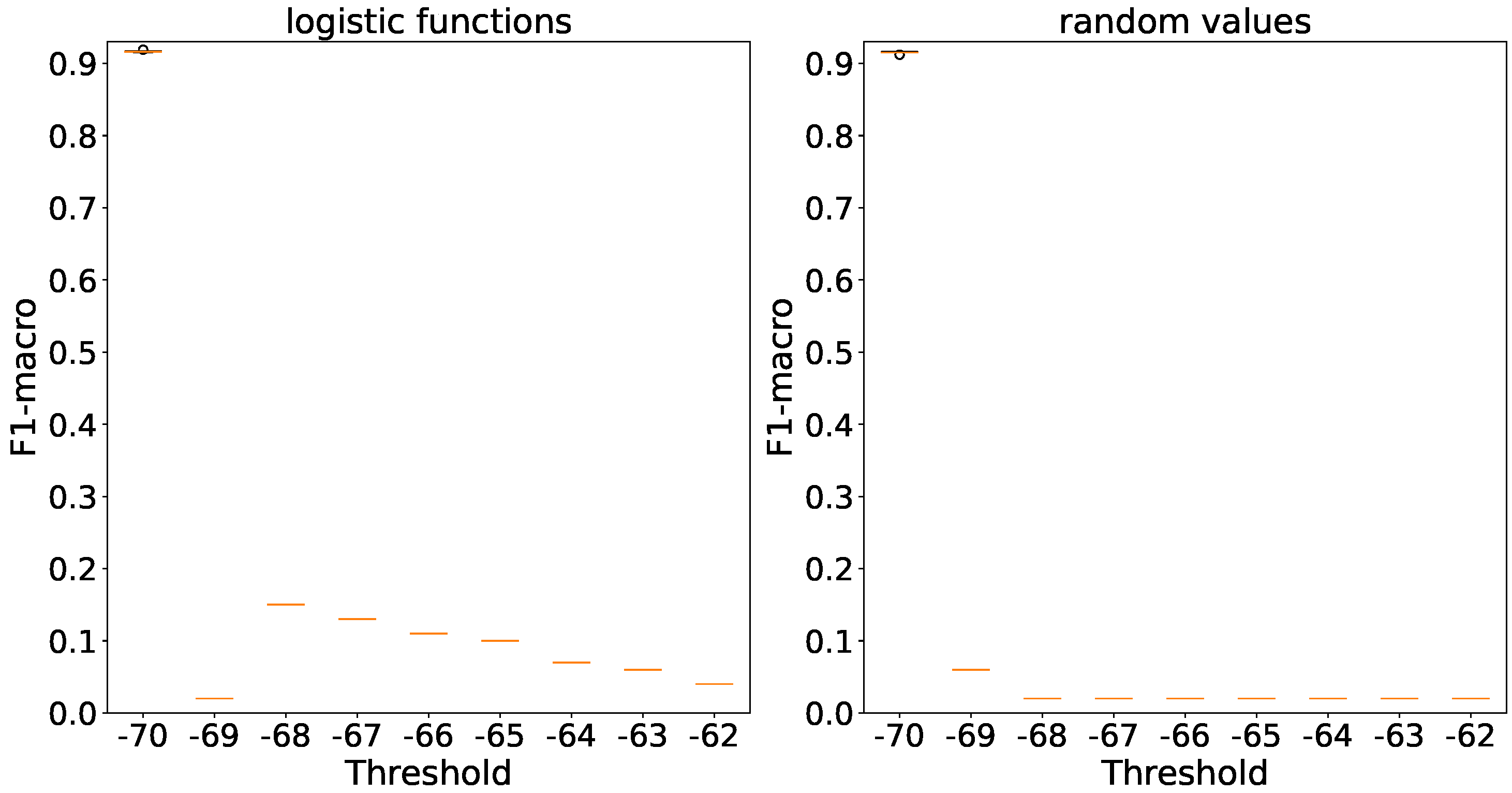
Increasing the threshold in both weight initialization methods results in a substantial reduction in accuracy based on Figure 16.

4.6. The influence of stochastic of input signal on the accuracy

During the experiment, we conducted a comparison between stochastic spike generation, where spikes are emitted according to a Poisson distribution at each discretization step of 0.1 ms, and non-stochastic spike generation, where they are uniformly generated within a time window determined by the corresponding input.

As before, accuracies were calculated several times, and the data were visualized using box plots. However, in order to eliminate the potential impact of weight initialization on the model’s accuracy, the weights were initialized once for all the attempts for both types of generators.

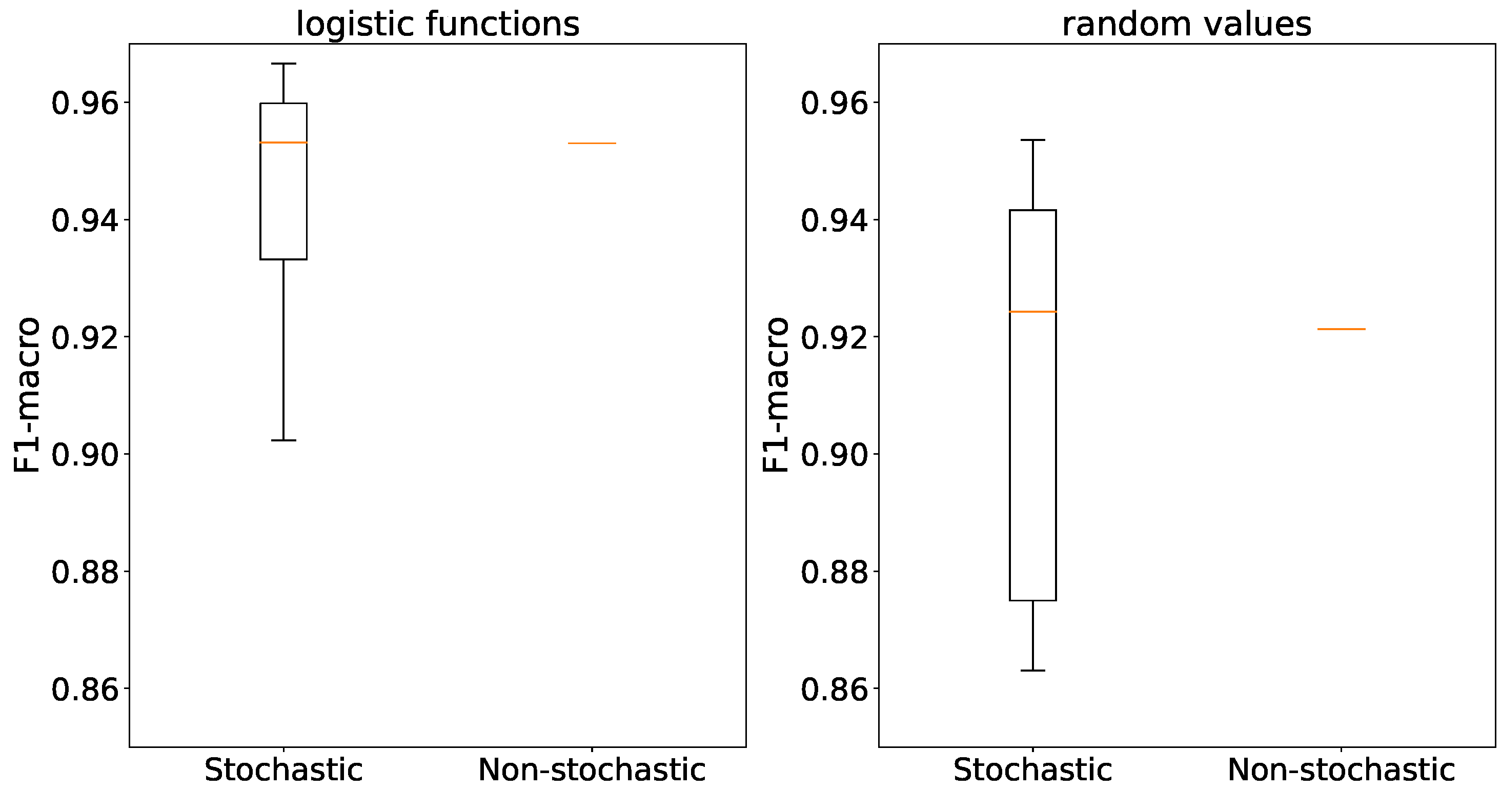
The use of stochastic generators results in outliers in accuracy, while the averages are comparable for both types of generators and both weight initialization methods as depicted in Figure 17.

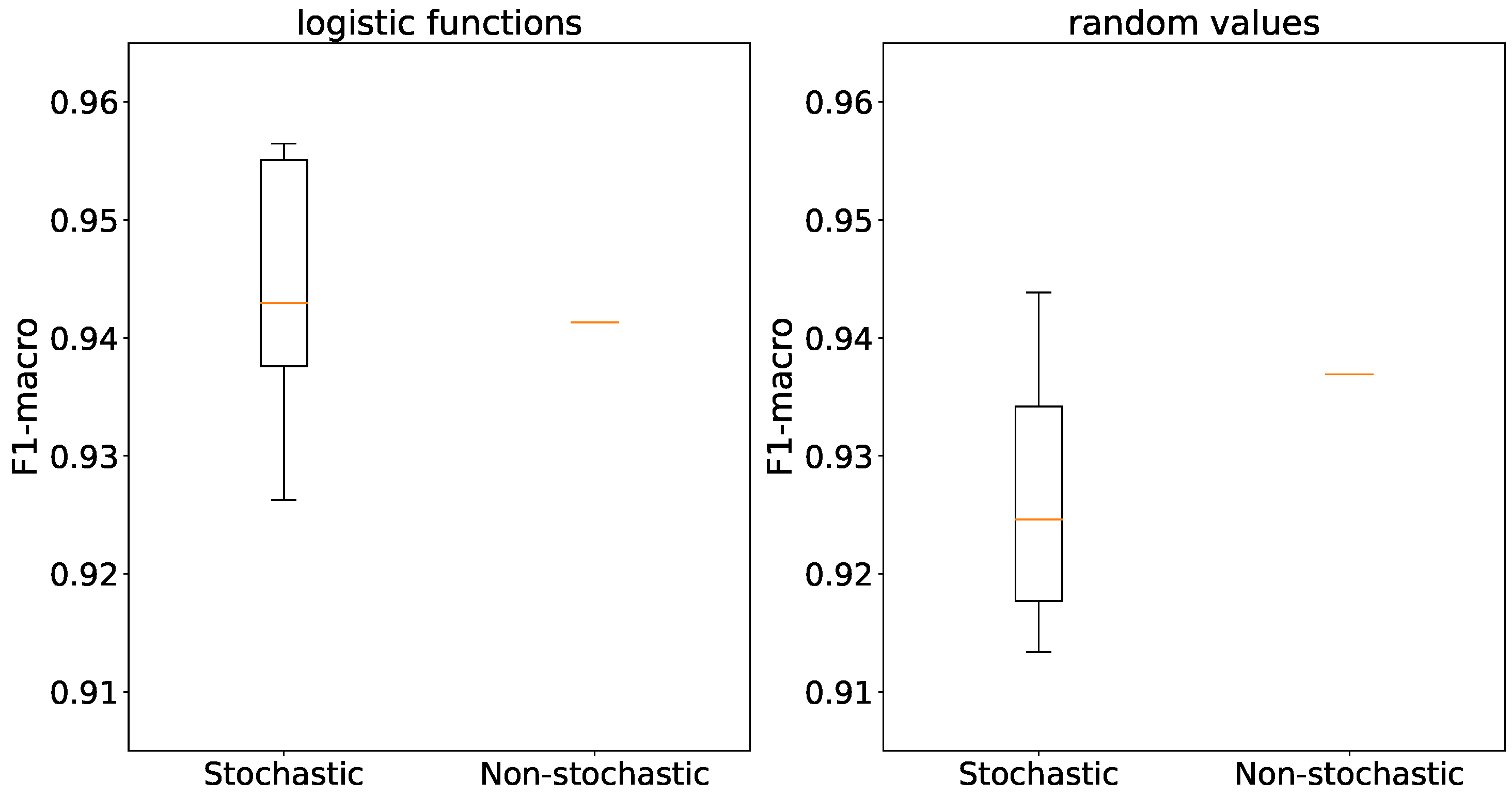
When using logistic functions, the accuracies of stochastic and non-stochastic generators are similar in line with Figure 18. However, in the case of random weight initialization, stochastic generators exhibit a considerable variance in accuracy compared to their non-stochastic counterparts.

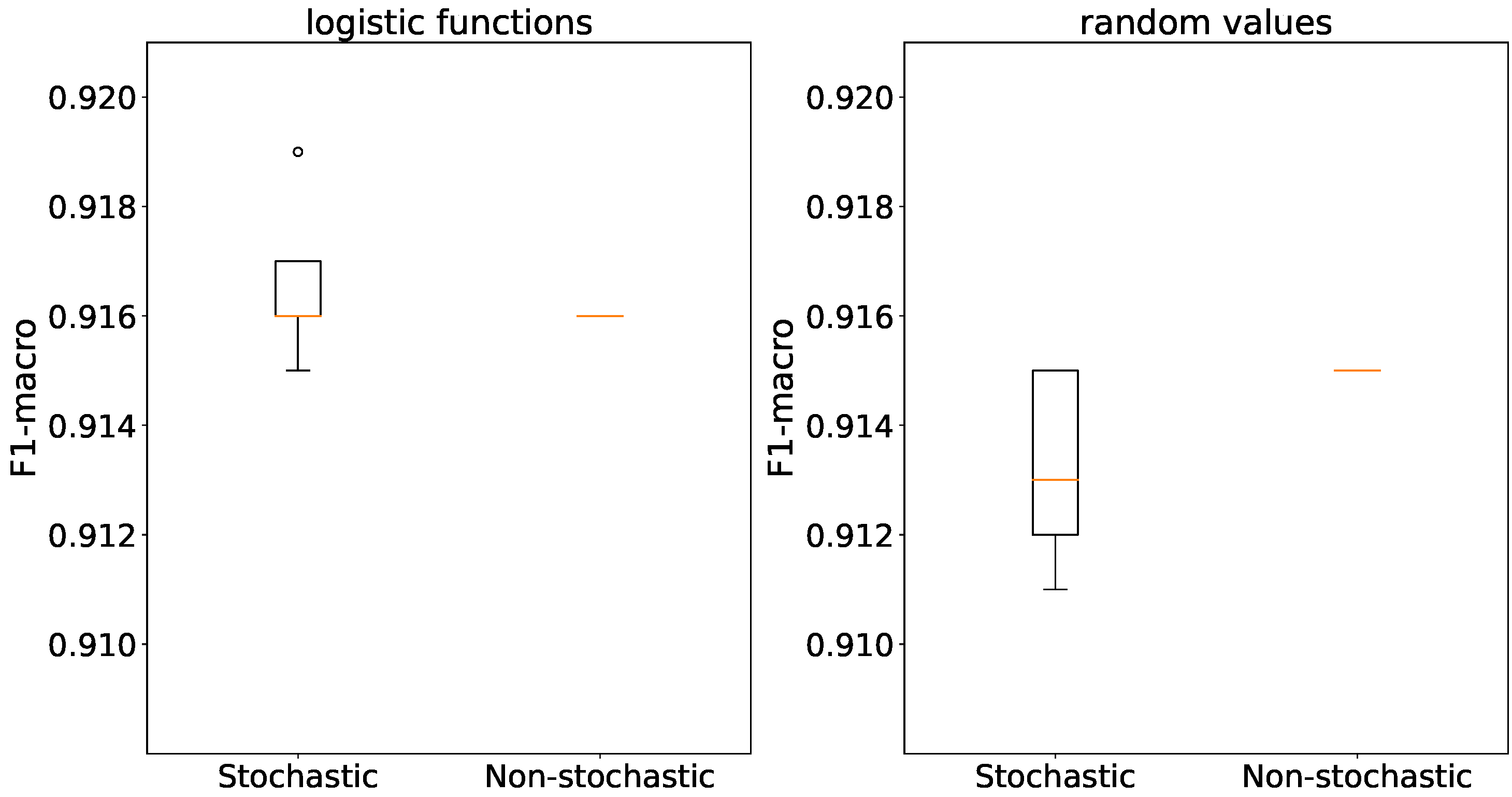
In in the context of Figure 16 accuracies are consistent for both initialization methods and generator types, with differences of no more than 1%. Non-stochastic generators completely remove accuracy deviation.

4.7. Efficiency of the proposed approach and comparison with other existing methods

In Table 1, we present the minimum spike counts required to achieve an average accuracy of 92% (referred to as Minimum Spike counts) and the spike counts needed to attain the highest achievable accuracy (referred to as Desired Spike counts) for each dataset for weight initialization method. The minimum and maximum F1-macro values across all attempts are linked to Desired Spike counts, which can be found in Figure 14 for the Fisher’s iris dataset, in Figure 15 for the Wisconsin Breast cancer dataset, in Figure 16 for the MNIST dataset. The table includes logistic regression and other existing spike-based approaches for comparative analysis. NC and PPX plasticities refer to the plasticity that models the conductance change of nanocomposite memristors [22] and the plasticity of highly-plastic poly-p-xylylene memristor [23] respectively. The table includes other existing methods for the MNIST dataset for comparison, whose accuracies were obtained using the complete training dataset.

Table 1. Comparison of accuracies with both weight initialization methods.

Weights	Spike counts		Performance
Weights	Minimum	Desired	Min	Max
Fisher’s Iris
Logistic functions	26	312	0.95	0.96
Random values	52	312	0.93	0.97
Logistic regression			0.93	0.97
STDP based approach on rate and temporal input encoding [24]			0.95	1.0
SpikeProp and Theta Neuron BP [25]			0.96	0.98
2-layer SNN with NC or PPX plasticity [26]			0.93	1.0
Wisconsin Breast Cancer
Logistic functions	3	8	0.94	0.97
Random values	2	24	0.94	0.97
Logistic regression			0.92	0.95
STDP based approach on rate and temporal input encoding [24]			0.88	0.92
SpikeProp and Theta Neuron BP [25]			0.97	0.99
2-layer SNN with NC or PPX plasticity [26]			0.88	0.96
MNIST
Logistic functions	160	160	0.92	0.92
Random values	160	160	0.92	0.92
Logistic regression			0.92	0.92
3-layer SNN with STDP [27]			0.95	0.95
3-layer SNN with STDP and BP [28]			0.98	0.98
2-layer SNN (100 neurons) with NC plasticity [29]			0.89	0.89

Table 2 presents the model parameters that result in the highest accuracies.

4.8. Discussion

Striving for low energy consumption of the prospective hardware implementation, our experiments were aimed at minimizing the number of processing elements in the layer, as well as the number of spikes in the network. However, input generators emitting too few spikes per input sample would lead to loss of information at the input encoding stage, while neurons emitting too few output spikes would lead to information loss at the decoding stage. Accordingly, lower neuron threshold makes samples of different classes more distinguishable by their output spike counts. Therefore, a processing element without a threshold, the adder, modelling an extreme case of a neuron with infinitely low threshold, allows one to obtain the lower bound on the number of input spikes sufficient for acceptable classification performance.

As a result, for all the three datasets used, we find that competitive accuracy can be achieved with as little as few hundred elements in the layer (furthermore, for the Wisconsin breast cancer dataset, just two neurons are sufficient, one neuron per class) and a few hundred input spikes per input vector.

Competitive accuracy was also achieved by the proposed approach on several other classification tasks. Our prior study [30] involving Free Spoken Digits data exhibited the accuracy of approximately 94%, while the Optical Recognition of Handwritten Digits data from our previous research [21] achieved the accuracy of around 92%. This shows the efficiency of the proposed approach for transforming input features into spike sequences.

Drawing weights from a random distribution rather than setting them on base of logsistic functions introduces more variability in accuracy, particularly in cases with limited datasets, such as Fisher’s Iris and Wisconsin Breast Cancer. Larger datasets, such as MNIST, yield more stable training results due to their larger number of examples.

The comparison of stochastic and non-stochastic spike generators did not reveal significant differences in the average accuracy between the two. However, the stochastic nature of the generators affects the accuracy variance, which increases for smaller datasets.

5. Conclusion

On a set of benchmarks – Fisher’s Iris, Wisconsin Breast Cancer and MNIST – we have empirically demonstrated the efficiency of the proposed non-trainable layer in transforming numeric input values into a less-dimensional space of counts of spikes emitted during a specified time window, allowing the subsequent decoding of the classes from the spike counts. We also show that the number of elements in the proposed layer, as well as the number of spikes needed for encoding an input sample, can be kept minimal without much accuracy loss. The highest classification accuracy achieved using this approach (see Table 1) are on par (in the case of Fisher’s Iris and MNIST) or exceed (in the case of Wisconsin Breast Cancer) the accuracy that logistic regression alone achieves on the respective tasks, thus proving the efficiency of the proposed layer as a feature extraction step. Synaptic weights of the non-trainable layer can be set random or on base of logistic functions; logistic functions reduce the result variability.

The obtained results lay a foundation for creating both efficient and economical spiking neural network topologies to be deployed on prospective biomorphic devices.

Author Contributions

Conceptualization, A.S. (Alexander Sboev); methodology, R.R.; software D.K., A.S. (Alexey Serenko); validation, D.K., A.S. (Alexey Serenko); formal analysis, A.S. (Alexey Serenko), V.I.; investigation, A.S. (Alexander Sboev), D.K., R.R.; resources, A.S. (Alexander Sboev), R.R.; data curation, A.S. (Alexey Serenko), V.P.; writing—original draft preparation, A.S. (Alexander Sboev), D.K.; writing—review and editing, A.S. (Alexander Sboev), R.R., A.S. (Alexey Serenko), V.I.; visualization, D.K., R.R.; supervision, A.S. (Alexander Sboev); project administration, A.S. (Alexander Sboev), R.R.; funding acquisition, A.S. (Alexander Sboev). All authors have read and agreed to the published version of the manuscript.

Funding

The study was supported by a grant from the Russian Science Foundation №23-11-00260, https://rscf.ru/project/23-11-00260/.

Data Availability Statement

The Fisher’s Iris and Wisconsin Breast Cancer datasets are publicly available through the Scikit-Learn Python library: https://scikit-learn.org/stable/. The MNIST dataset can be freely obtained from https://www.kaggle.com/datasets/oddrationale/mnist-in-csv.

Acknowledgments

Computational experiments were carried out using computing resources of the federal collective usage center Complex for Simulation and Data Processing for Mega-science Facilities at NRC “Kurchatov Institute”, http://ckp.nrcki.ru/.

Conflicts of Interest

The authors declare no conflict of interest.

Abbreviations

The following abbreviations are used in this manuscript:

BP	Backpropagation
MNIST	Modified National Institute of Standards and Technology
NC	Nanocomposite
SNN	Spiking neural network
STDP	Spike-timing-dependent plasticity
PE	Processing elements
PPX	Poly-p-xylylene

References

Diehl, P.U.; Pedroni, B.U.; Cassidy, A.; Merolla, P.; Neftci, E.; Zarrella, G. TrueHappiness: Neuromorphic emotion recognition on TrueNorth. In Proceedings of the 2016 International Joint Conference on Neural Networks (IJCNN), 2016; pp. 4278–4285. [Google Scholar] [CrossRef]
Davies, M.; Srinivasa, N.; Lin, T.H.; Chinya, G.; Cao, Y.; Choday, S.H.; Dimou, G.; Joshi, P.; Imam, N.; Jain, S.; et al. Loihi: A neuromorphic manycore processor with on-chip learning. IEEE Micro 2018, 38, 82–99. [Google Scholar] [CrossRef]
Pei, J.; Deng, L.; Song, S.; Zhao, M.; Zhang, Y.; Wu, S.; Wang, G.; Zou, Z.; Wu, Z.; He, W.; et al. Towards artificial general intelligence with hybrid Tianjic chip architecture. Nature 2019, 572, 106–111. [Google Scholar] [CrossRef]
Wan, W.; Kubendran, R.; Schaefer, C.; Eryilmaz, S.B.; Zhang, W.; Wu, D.; Deiss, S.; Raina, P.; Qian, H.; Gao, B.; et al. A compute-in-memory chip based on resistive random-access memory. Nature 2022, 608, 504–512. [Google Scholar] [CrossRef] [PubMed]
Kim, D.; Shin, J.; Kim, S. Implementation of reservoir computing using volatile WOx-based memristor. Applied Surface Science 2022, 599, 153876. [Google Scholar] [CrossRef]
Yang, J.; Cho, H.; Ryu, H.; Ismail, M.; Mahata, C.; Kim, S. Tunable synaptic characteristics of a Ti/TiO2/Si memory device for reservoir computing. ACS Applied Materials & Interfaces 2021, 13, 33244–33252. [Google Scholar]
Lin, Y.; Liu, J.; Shi, J.; Zeng, T.; Shan, X.; Wang, Z.; Zhao, X.; Xu, H.; Liu, Y. Nitrogen-induced ultralow power switching in flexible ZnO-based memristor for artificial synaptic learning. Applied Physics Letters 2021, 118. [Google Scholar] [CrossRef]
Díaz-Pernil, D.; Pena-Cantillana, F.; Gutiérrez-Naranjo, M.A. A parallel algorithm for skeletonizing images by using spiking neural P systems. Neurocomputing 2013, 115, 81–91. [Google Scholar] [CrossRef]
Ryu, H.; Kim, S. Implementation of a reservoir computing system using the short-term effects of Pt/HfO2/TaOx/TiN memristors with self-rectification. Chaos, Solitons & Fractals 2021, 150, 111223. [Google Scholar] [CrossRef]
Mikhaylov, A.; Pimashkin, A.; Pigareva, Y.; Gerasimova, S.; Gryaznov, E.; Shchanikov, S.; Zuev, A.; Talanov, M.; Lavrov, I.; Demin, V.; et al. Neurohybrid memristive CMOS-integrated systems for biosensors and neuroprosthetics. Frontiers in neuroscience 2020, 14, 358. [Google Scholar] [CrossRef] [PubMed]
Wang, Q.; Pan, G.; Jiang, Y. An Ultra-Low Power Threshold Voltage Variable Artificial Retina Neuron. Electronics 2022, 11, 365. [Google Scholar] [CrossRef]
Lee, Y.; Mahata, C.; Kang, M.; Kim, S. Short-term and long-term synaptic plasticity in Ag/HfO2/SiO2/Si stack by controlling conducting filament strength. Applied Surface Science 2021, 565, 150563. [Google Scholar] [CrossRef]
Wu, X.; Dang, B.; Wang, H.; Wu, X.; Yang, Y. Spike-Enabled Audio Learning in Multilevel Synaptic Memristor Array-Based Spiking Neural Network. Advanced Intelligent Systems 2022, 4, 2100151. [Google Scholar] [CrossRef]
Vlasov, D.; Davydov, Y.; Serenko, A.; Rybka, R.; Sboev, A. Spoken digits classification based on Spiking neural networks with memristor-based STDP. In Proceedings of the 2022 International Conference on Computational Science and Computational Intelligence (CSCI), 2022; pp. 330–335. [Google Scholar]
Vlasov, D.; Minnekhanov, A.; Rybka, R.; Davydov, Y.; Sboev, A.; Serenko, A.; Ilyasov, A.; Demin, V. Memristor-based spiking neural network with online reinforcement learning. Neural Networks 2023, 166, 512–523. [Google Scholar] [CrossRef] [PubMed]
Matsukatova, A.N.; Iliasov, A.I.; Nikiruy, K.E.; Kukueva, E.V.; Vasiliev, A.L.; Goncharov, B.V.; Sitnikov, A.V.; Zanaveskin, M.L.; Bugaev, A.S.; Demin, V.A.; et al. Convolutional Neural Network Based on Crossbar Arrays of (Co-Fe-B) x (LiNbO3) 100- x Nanocomposite Memristors. Nanomaterials 2022, 12, 3455. [Google Scholar] [CrossRef] [PubMed]
Shahsavari, M.; Boulet, P. Parameter exploration to improve performance of memristor-based neuromorphic architectures. IEEE Transactions on Multi-Scale Computing Systems 2017, 4, 833–846. [Google Scholar] [CrossRef]
Lukoševičius, M.; Jaeger, H. Reservoir computing approaches to recurrent neural network training. Computer science review 2009, 3, 127–149. [Google Scholar] [CrossRef]
Velichko, A. Neural Network for Low-Memory IoT Devices and MNIST Image Recognition Using Kernels Based on Logistic Map. Electronics 2020, 9. [Google Scholar] [CrossRef]
Sboev, A.; Kunitsyn, D.; Serenko, A.V.; Rybka, R.B. A spiking neural network with fixed synaptic weights based on logistic maps for a classification task. In Proceedings of the The 6th International Workshop on Deep Learning in Computational Physics, 2022; p. 10. [Google Scholar] [CrossRef]
Sboev, A.G.; Serenko, A.V.; Kunitsyn, D.E.; Rybka, R.B.; Putrolaynen, V.V. Towards Solving Classification Tasks Using Spiking Neurons with Fixed Weights. In Proceedings of the International Conference on Neuroinformatics, 2023; pp. 102–110. [Google Scholar] [CrossRef]
Demin, V.; Nekhaev, D.; Surazhevsky, I.; Nikiruy, K.; Emelyanov, A.; Nikolaev, S.; Rylkov, V.; Kovalchuk, M. Necessary conditions for STDP-based pattern recognition learning in a memristive spiking neural network. Neural Networks 2021, 134, 64–75. [Google Scholar] [CrossRef] [PubMed]
Minnekhanov, A.A.; Shvetsov, B.S.; Martyshov, M.M.; Nikiruy, K.E.; Kukueva, E.V.; Presnyakov, M.Y.; Forsh, P.; Rylkov, V.V.; Erokhin, V.V.; Demin, V.A.; et al. On the resistive switching mechanism of parylene-based memristive devices. Organic Electronics 2019. [Google Scholar] [CrossRef]
Sboev, A.; Serenko, A.; Rybka, R.; Vlasov, D. Solving a classification task by spiking neural network with STDP based on rate and temporal input encoding. Mathematical Methods in the Applied Sciences 2020, 43, 7802–7814. [Google Scholar] [CrossRef]
Paugam-Moisy, H.; Bohte, S.M. Computing with spiking neuron networks. Handbook of natural computing 2012, 1, 1–47. [Google Scholar]
Sboev, A.; Vlasov, D.; Rybka, R.; Davydov, Y.; Serenko, A.; Demin, V. Modeling the Dynamics of Spiking Networks with Memristor-Based STDP to Solve Classification Tasks. Mathematics 2021, 9. [Google Scholar] [CrossRef]
Li, J.; Xu, H.; Sun, S.Y.; Li, N.; Li, Q.; Li, Z.; Liu, H. In Situ Learning in Hardware Compatible Multilayer Memristive Spiking Neural Network. IEEE Transactions on Cognitive and Developmental Systems 2021, 14, 448–461. [Google Scholar] [CrossRef]
Gerlinghoff, D.; Luo, T.; Goh, R.S.M.; Wong, W.F. Desire backpropagation: A lightweight training algorithm for multi-layer spiking neural networks based on spike-timing-dependent plasticity. Neurocomputing 2023, 560, 126773. [Google Scholar] [CrossRef]
Demin, V.A.; Nekhaev, D.V.; Surazhevsky, I.A.; Nikiruy, K.E.; Emelyanov, A.V.; Nikolaev, S.N.; Rylkov, V.V.; Kovalchuk, M.V. Necessary conditions for STDP-based pattern recognition learning in a memristive spiking neural network. Neural Networks 2021, 134, 64–75. [Google Scholar] [CrossRef]
Sboev, A.; Kunitsyn, D.; Balykov, M.A. Spoken Digits Classification Using a Spiking Neural Network with Fixed Synaptic Weights. 2023 Annual International Conference on Brain-Inspired Cognitive Architectures for Artificial Intelligence, the 14th Annual Meeting of the BICA Society (in press).

Figure 1. The MNIST dataset.

Figure 2. Visualization of: A — Fisher’s Iris data, B - Wisconsin Breast (Diagnostic) Cancer data.

Figure 3. The topology of the proposed approach.

Figure 4. The impact of the volume of the used MNIST training data on model accuracy.

Figure 5. The accuracy dependence on the length of the time window on the Fisher’s Iris data.

Figure 6. The accuracy dependence on the length of the time window on the Breast Cancer Wisconsin (Diagnostic) data.

Figure 7. The accuracy dependence on the length of time window in the MNIST data.

Figure 8. The accuracy dependence on the number of processing elements on the Fisher’s Iris data.

Figure 9. The accuracy dependence on the number of processing elements on the Breast Cancer Wisconsin (Diagnostic) data.

Figure 10. The accuracy dependence on the number of processing elements in the MNIST data.

Figure 11. The dependence between accuracy and the number of spikes on the Fisher’s Iris data.

Figure 12. The dependence between accuracy and the number of spikes generated by the generators on the Breast Cancer Wisconsin (Diagnostic) data.

Figure 13. The dependence between accuracy and the number of spikes generated by the generators on the MNIST data.

Figure 14. The dependence between accuracy and the threshold potential of spiking neurons on the Fisher’s Iris data.

Figure 15. The dependence between accuracy and the threshold potential of spiking neurons on the Breast Cancer Wisconsin (Diagnostic) data.

Figure 16. The dependence between accuracy and the threshold potential of spiking neurons on the MNIST data.

Figure 17. The dependence between accuracy and spike generation method on the Fisher’s Iris data.

Figure 18. The dependence between accuracy and spike generation method on the Breast Cancer Wisconsin (Diagnostic) data.

Figure 19. The dependence between accuracy and spike generation method on the MNIST data.

Table 2. Parameter values of the models that achieved the best performance on each dataset and weight initialization.

Weights	Number of PE	Spike counts	$V_{th}$ , mV	Time window, ms
Fisher’s Iris
Logistic functions	3	312	-70	5200
Random values	3	312	-70	5200
Wisconsin Breast Cancer
Logistic functions	16	8	-69.94	200
Random values	16	24	-69.8	200
MNIST
Logistic functions	350	160	-70	200
Random values	350	160	-70	200

Disclaimer/Publisher’s Note: The statements, opinions and data contained in all publications are solely those of the individual author(s) and contributor(s) and not of MDPI and/or the editor(s). MDPI and/or the editor(s) disclaim responsibility for any injury to people or property resulting from any ideas, methods, instructions or products referred to in the content.

© 2023 by the authors. Licensee MDPI, Basel, Switzerland. This article is an open access article distributed under the terms and conditions of the Creative Commons Attribution (CC BY) license (http://creativecommons.org/licenses/by/4.0/).

Copyright: This open access article is published under a Creative Commons CC BY 4.0 license, which permit the free download, distribution, and reuse, provided that the author and preprint are cited in any reuse.

MDPI Initiatives

Important Links

Choose an area of interest and we will send you notifications of new preprints at your preferred frequency.

Disclaimer