Modeling Autonomous Vehicle Responses to Novel Observations using Hierarchical Cognitive Representations Inspired Active Inference

Preprint

Article

Modeling Autonomous Vehicle Responses to Novel Observations using Hierarchical Cognitive Representations Inspired Active Inference

Altmetrics

Downloads

124

Views

Comments

A peer-reviewed article of this preprint also exists.

This version is not peer-reviewed

Submitted:

27 November 2023

Posted:

28 November 2023

You are already at the latest version

Alerts

Abstract

Equipping autonomous agents for dynamic interaction and navigation is a significant challenge in intelligent transportation systems. This study aims to address this by implementing a brain-inspired model for decision-making in autonomous vehicles. We employ active inference, a Bayesian approach that models decision-making processes similar to the human brain, focusing on the agent's preferences and the principle of free energy. This approach is combined with imitation learning to enhance the vehicle's ability to adapt to new observations and make human-like decisions. The research involved developing a multi-modal self-awareness architecture for autonomous driving systems and testing this model in driving scenarios, including abnormal observations. The results demonstrated the model's effectiveness in enabling the vehicle to make safe decisions, particularly in unobserved or dynamic environments. The study concludes that the integration of active inference with imitation learning significantly improves the performance of autonomous vehicles, offering a promising direction for future developments in intelligent transportation systems.

Keywords:

Subject: Computer Science and Mathematics - Artificial Intelligence and Machine Learning

1. Introduction

Autonomous driving systems (ADS) are a rapidly developing field that has the potential to revolutionize transportation in smart cities [1,2]. One of the main challenges that ADS face is their ability to adapt to novel observations in a constantly changing environment. This challenge is due to the inherent complexity and uncertainty of the real world, which may lead to unexpected and unpredictable situations.

Driving scenarios involve multiple unpredictable factors, such as diverse driver behaviors and environmental fluctuations. These challenges require a shift from traditional rule-based learning models [3] to adaptive and cognitive entities, enabling autonomous vehicles (AVs) to navigate through complex and unpredictable terrains effectively.

Cognitive learning is a promising approach to tackle the challenge of adapting to novel situations in a dynamic environment [4]. This approach aligns with the principles of Bayesian brain learning [5], which suggests that the human brain operates as a Bayesian inference system, constantly updating its probabilistic models to perform a wide range of cognitive tasks such as perception, planning, and learning. This allows autonomous agents to update their beliefs about the external world in response to novel observations. In the context of ADS, integrating these concepts leads to the emergence of vehicles with a cognitive hierarchy. One of the open questions in this area is to what extent autonomous vehicles can move beyond mere rule-following or imitating prior sub-optimal experiences. The hierarchy principles go beyond rule-based behaviour, allowing autonomous vehicles to perceive their surroundings through probabilistic perception, infer causal structures, predict future states, and act with agency. This provides an adaptive learning agent that continuously enhances its cognitive models through experiences.

At the heart of the cognitive hierarchy of AVs is the critical role played by Generative Models (GMs) [6]. These models allow AVs to comprehend the underlying dynamics of the environment, which, in turn, empowers them to anticipate future behaviour and engage in proactive decision-making [7]. By relying on GMs, AVs go beyond simple perception and use predictive inferences to represent the agent’s beliefs about the world. Furthermore, the autonomous agent must be able to plan a sequence of actions that will help it gain information and reduce uncertainty about the surroundings.

Active inference [8], grounded in the Bayesian brain learning paradigm, is a computational framework bridging the gap between perception and action. It suggests that an intelligent agent, such as an autonomous vehicle (AV), should not just passively observe its environment but actively engage in exploratory actions to refine its internal probabilistic models. This is achieved through a continuous cycle of observation, belief updating, and action selection. The process begins with perception, where the AV uses an array of sensors to engage in multisensory and multimodal observation of its surroundings, accumulating sensory evidence about the external world. This sensory evidence is then integrated into a probabilistic model, commonly represented as a belief distribution. The belief distribution encapsulates the vehicle’s understanding of the environment, encompassing not only the current state but also a spectrum of potential states, inherently acknowledging uncertainty.

In active inference, messages are propagated between different layers of a probabilistic model, allowing for the exchange of information. These messages are probabilistic updates that convey crucial insights about the environment’s dynamics and help to refine the AV’s internal probabilistic representation. In addition, active inference introduces the concept of action selection guided by inference. Rather than responding automatically, the AV engages in a deliberate action-planning process. The agent chooses actions that maximize the expected sensory evidence while also accounting for their internal beliefs and uncertainty, contributing to the minimization of free energy [9].

Furthermore, active inference is a powerful technique that enables autonomous agents to develop a sense of self-awareness [10]. By continuously comparing their sensory observations with their internal beliefs, these agents strive to minimize free energy and gain an understanding of their own knowledge and the limits of their perception. This self-awareness allows them to recognize when to seek additional information through exploratory actions and when they can rely on their existing knowledge to make decisions. Simply put, active inference helps autonomous agents become cognitively self-aware while also compelling them to minimize the difference between their internal models and external reality. This allows them to adapt and learn from their environment, make better decisions, and navigate uncertain and complex situations.

Motivated by the previous discussion, we propose a cognitive hierarchical framework for modelling AV responses to abnormalities, such as novel observations, during a lane-changing scenario, based on Active Inference. The AV, equipped with self-awareness, should learn to self-drive in a dynamic environment while interacting with other participants. The proposed framework consists of two essential computational modules: a perception module and an adapting learning module. The perception module analyzes the sensory signals and creates a model based on the observed interaction between the participants in a dynamic environment. This allows the AV to perceive the external world as a bundle of exteroceptive and proprioceptive sensations from multiple sensory modalities and to integrate information from different sensory inputs and match them appropriately. In this work, the AV integrates proprioceptive stimuli (i.e., AV’s positions) with exteroceptive stimuli (i.e., the relative distance between AV and another object) and describes the integration process using Bayesian inference. The adapting learning module consists of a world model and an active model. The world model is essential to the cognitive processes of perception, inference, prediction, and decision-making in active inference systems. It bridges the agent’s internal representation and interactions with the external environment, enabling the agent to adapt its behaviour to uncertain scenarios. The active model plans the AV’s actions as inferred from the world model in terms of minimizing the cost function due to the uncertainty (i.e., unseen situation), which components are linked by the active inference process.

The main contributions of this paper can be summarized as follows:

We present a comprehensive hierarchical cognitive framework for autonomous driving, addressing the challenge of responding to novel observations in dynamic environments. This framework marks a fundamental shift from rule-based learning models to cognitive entities capable of AV navigating unseen terrains.
The proposed framework firmly grounded the principles of Bayesian learning, enabling ADS to adapt its probabilistic models continually. This adaptation is essential for the continuous improvement of the cognitive model through experiences. Consequently, an AV can consistently update its beliefs regarding the surroundings.
We expand upon a global dictionary to incrementally develop a dynamic world model during the learning process. This world model efficiently structures newly acquired environmental knowledge, enhancing AV perception and decision-making.
Through active inference, the proposed approach equipped the AV with a sense of self-awareness by continually comparing sensory observations with internal beliefs and aiming to minimize free energy. This self-awareness enables them to make informed decisions about seeking additional information through exploratory actions and when to rely on existing knowledge.
The dynamic interaction between the ego AV and its environment, as facilitated by active inference, forms the basis for adaptive learning. This adaptability augments AV’s decision-making capabilities, positioning it as a cognitive entity capable of navigating confidently and effectively in uncertain and complex environments.

2. Related Works

One of the most pivotal advancements in intelligent transportation is the development of autonomous driving (AD). AVs are defined as agents capable of navigating from one location to another without human control. These vehicles perceive their surroundings using a variety of sensors, processing this information to operate independently of human intervention [11]. AD involves addressing challenges in perception and motion planning, particularly in environments with dynamic objects. The complex interactions among multiple agents pose significant challenges, primarily due to the unpredictability of their future states. Most model-based AD strategies require the manual creation of driving policy models [12,13], or they incorporate safety assessments to assisst human drivers [14,15].

In recent years, there has been a substantial increase in the demand for AVs that can imitate human behavior. Advances in ADS have opened up a wide range of potential applications where an agent is required to make intelligent decisions and execute realistic motor actions in diverse scenarios. A key aspect of future developments in AVs hinges on the agent’s ability to perform as an expert in similar situations. Research indicates that utilizing expert knowledge is more effective and efficient than starting from scratch [16,17,18]. One practical method for transferring this expertise is through providing optimal demonstrations of the desired behavior for the learning agent

(L)

to replicate [19].

Imitation Learning (IL) involves acquiring skills or behaviors by observing an expert perform a specific task. This approach is vital to the development of machine intelligence, drawing inspiration and foundational concepts from cognitive science. IL has long been considered a crucial component in the evolution of intelligent agents [17].

Imitation Learning (IL) is similar to standard supervised learning, but instead of pairing features with labels, it pairs states with actions. In IL, a state represents the agent’s current situation and the condition of any target object involved. The IL process typically begins with collecting example demonstrations from an expert agent

(E)

, which are then translated into state-action pairs. However, simply learning a direct state-to-action relationship isn’t enough to ensure the desired behavior. Challenges such as errors in demonstration collection or a lack of comprehensive demonstrations can arise [20]. Additionally, the learner’s task might slightly differ from the demonstrated one due to environmental changes, obstacles, or targets. Therefore, IL often includes a step where the learner applies the learned actions and adjusts its approach based on task performance.

The existing works of the IL approach for driving can handle simple driving tasks such as lane following [21,22]. However, if the agent is dealing with a new environment or a more complicated task (such as lane-changing), the human driver must take control, or the system ultimately fails [23,24]. More specifically, a typical IL procedure is direct learning, where the main goal is to learn a mapping from states to actions that mimic the demonstrator explicitly [25,26]. Direct learning methods are categorized into classification methods when the learner’s actions can be classified into discrete classes [27,28], and regression methods which are used to learn actions in a continuous space [29]. Direct learning often fails to reproduce proper behavior due to issues such as insufficient demonstrations or the need to perform different tasks in changing environments. Additionally, indirect learning can complement direct approaches by refining the policies based on sub-optimal expert demonstrations [30].

The primary limitations of IL include the policy’s inability to surpass the expert’s suboptimal performance and its susceptibility to distributional shifts [31]. Consequently, IL often incorporates an additional step where the learning agent refines the estimated policy according to its current context. This self-improvement process can be guided by measurable rewards or learning from specific instances.

Many of these approaches fall under the umbrella of reinforcement learning (RL) methods. RL enables the encoding of desired behaviors, such as reaching a target and avoiding collisions, and does not solely rely on perfect expert demonstrations. Additionally, RL focuses on maximizing the expected return over an entire trajectory, unlike IL, which treats each observation independently [32]. This conceptual difference often positions RL as superior to IL. However, without prior knowledge from an expert, the RL learning agent may struggle to identify desired behaviors in environments with sparse rewards [33]. Furthermore, even when RL successfully maximizes rewards, the resulting policy may not align with the behaviors anticipated by the reward designer. The trial-and-error nature of RL also necessitates task-specific reward functions, which can be complex and challenging to define in many scenarios.

Learning approaches like IL and RL can be complex without adequate representation or model learning from the environment. To address these challenges, autonomous systems often adopt an incremental learning approach. This method enables the agent to acquire new knowledge while retaining previously learned information [34,35]. As a result, the learning agent becomes capable of processing and understanding new situations that it encounters over time.

3. Proposed Framework

The hierarchical cognitive schematic introduced in Figure 1 comprises several modules that form a cognitive cycle, preparing an Autonomous Vehicle (AV) to perceive its environment and interact with its surroundings. When the system faces a new situation (i.e., novel sensorial input), an AV interprets the external world by formulating and testing hypotheses about its evolution. It generates predictions based on prior knowledge acquired from past experiences, performs actions based on its beliefs, observes the outcomes, and refines the beliefs accordingly. The different modules in the architecture can be likened to different areas of the biological brain, each one handling particular functionalities. Some parts are responsible for sensory perception, while others are dedicated to planning and decision-making. All parts are interconnected and operate together. The cognitive model is characterized by inferences across different modules that enable it to predict the perceptual outcomes of actions. Moreover, the model must utilize these representations to minimize prediction errors and predict how sensory signals change under specific actions. The following sections present a detailed description of the different modules involved in the architecture.

3.1. Perception Module

An autonomous vehicle (AV) to effectively operate in its environment requires a perception module that can learn how it interacts with other dynamic entities. This module takes in multi-sensorial information to identify causalities among the data perceived by the agent. Using various sensors to gather information is vital in constructing a model capable of predicting the agent’s dynamics for motion planning. The ability to perceive multimodal stimuli is crucial, as it provides multimodal information under different conditions to augment the scene library of the ADS.

To accurately predict how information will be perceived, the module integrates exteroceptive and proprioceptive perceptions to formulate a contextual viewpoint. This viewpoint includes both internal and external perceptions of the agent. The primary aim is to use this information to predict subsequent internal or external states. To achieve this, the movements of both the AV and other participants are simulated at each instant through interacting rules dependent on their positions and motions, generating coupled trajectory data. Analyzing this multisensory data helps encode the dynamic interaction of the associated agents as probabilities into a coupled Generative Dynamic Bayesian Network (C-GDBN). The resulting dynamic interaction model is self-aware, capable of identifying abnormalities, and incrementally learning new interacting behaviours derived from an initial one, influencing the agent’s decision-making.

3.2. Adaptive Learning Module

In addition to the perception module, we have developed an adaptive learning module that enhances the AV’s ability to respond to its surroundings. This module continuously analyzes the agent’s interactions with the environment and adapts the AV’s responses accordingly by acquiring incremental knowledge of the evolving context. This approach ensures the AV can proactively anticipate changes, make better decisions, and respond adeptly. Integrating the adaptive learning module represents a significant step forward in promoting an adaptive interaction between the AV and its surroundings. The module comprises two components: the World Model and the Active Model.

3.2.1. World Model

The World Model (WM) acts like a simulator in the brain, providing insights into how the brain learns to execute sensorimotor behaviors [36]. In the proposed architecture, the WM is formulated using generative models, leveraging interactive experiences derived from multimodal sensory information. Initially, the WM is established by the Situation Model (SM), serving as a fundamental input module (see Figure 2). The SM, represented as a Coupled GDBN (C-GDB), models the motions and dynamic interactions between two entities in the environment, enabling the estimation of the vehicles’ intentions through probabilistic reasoning. This constructed C-GDBN demonstrates the gathered sub-optimal information concerning the interaction of an expert AV (

E

) with one vehicle (

V 1

) in the same lane, where

E

changes lanes to overtake

V 1

without a collision (comprehensive details on structuring the SM can be found in our previous work [37]). To initialize the WM by using the provided SM, we transfer the knowledge of

E

to a First-Person perspective, where an intelligent vehicle

(L)

learns by interacting with its environment via observing the

E

’s behaviour to integrate the gain knowledge into its understanding of the surroundings.

The First-Person model (FP-M) establishes a dynamic model that shifts

L

from a third-person viewpoint to a first-person experience. This allows

L

to perceive driving tasks as

E

does, enhancing its imitation accuracy. Such a perspective empowers

L

to react promptly during interactions with

V 1

. FP-M’s structure is derived by translating the hierarchical levels of SM into the FP context (as illustrated in Figure 3). The top level of hierarchy in FP-M denotes pre-established configurations

(\tilde{D})

from the dynamic behaviour of how

E

and

V 1

interact in the environment. Each configuration represents a joint discrete state as:

{\tilde{D}}_{k} = f ({\tilde{D}}_{k - 1}) + w_{k},

(1)

where

{\tilde{D}}_{k}

is a latent discrete state evolving from the previous state

{\tilde{D}}_{k - 1}

by a non-linear state evolution function

f (\cdot)

representing the transition dynamic model and by a Gaussian process noise

w_{k} \sim N (0, Q)

. The discrete state variables

{\tilde{D}}_{k} = [S_{k}^{E}, S_{k}^{V 1}]

represent jointly the discrete states of

E

and

V 1

where

S_{k}^{E} \in 𝓢^{E}

S_{k}^{V 1} \in 𝓢^{V 1}

{\tilde{D}}_{k} \in 𝓓

, and

𝓢^{E}

and

𝓢^{V 1}

are learned according to the approach discussed in [38], while

𝓓 = {{\tilde{D}}_{1}, {\tilde{D}}_{2}, \dots, {\tilde{D}}_{m}}

is the set that represents the dictionary consisting of all the possible joint discrete states (i.e., configurations) and m is the total number of configurations. Therefore, by tracking the evolution of these configurations over time, it is possible to determine the transition matrix that quantifies the likelihood of transitioning from one configuration to the next, as defined by:

Π = [\begin{matrix} P ({\tilde{D}}_{1} | {\tilde{D}}_{1}), & \dots, & P ({\tilde{D}}_{1} | {\tilde{D}}_{m}) \\ ⋮ & ⋱ & ⋮ \\ P ({\tilde{D}}_{m} | {\tilde{D}}_{1}), & \dots, & P ({\tilde{D}}_{m} | {\tilde{D}}_{m}) \end{matrix}]

(2)

where

Π \in R^{m, m}

P ({\tilde{D}}_{i} | {\tilde{D}}_{j})

represents the transition probability from configuration i to configuration j and

\sum_{k = 1}^{m} P (D_{i} | {\tilde{D}}_{k}) = 1

\forall i

The hidden continuous states

(\tilde{X})

in the FP-M represent the dynamic interaction in terms of generalized relative distance consisting of relative distance and relative velocity, which is defined as:

{\tilde{X}}_{k} = [{\tilde{X}}_{k}^{E} - {\tilde{X}}_{k}^{V 1}] = [(x_{k}^{E} - x_{k}^{V 1}), ({\dot{x}}_{k}^{E} - {\dot{x}}_{k}^{V 1})] .

(3)

The initialization is based on SM where the continuous latent state

{\tilde{X}}_{k} = [{\tilde{X}}_{k}^{E}, {\tilde{X}}_{k}^{V 1}] \in R^{n_{x}}

represent a joint belief state where

{\tilde{X}}_{k}^{E}

and

{\tilde{X}}_{k}^{V 1}

denote the hidden generalized states (GSs) of

E

and

V 1

, respectively. The GSs consist of the vehicles’ position and velocity where

{\tilde{X}}_{k}^{i} = [x_{k}^{i}, y_{k}^{i}, {\dot{x}}_{k}^{i}, {\dot{y}}_{k}^{i}]

and

i \in {E, V 1}

. The continuous variables

{\tilde{X}}_{k}

evolve from the previous state

{\tilde{X}}_{k - 1}

by the linear state function

g (\cdot)

and by a Gaussian noise

w_{k}

, as follow:

{\tilde{X}}_{k} = g ({\tilde{X}}_{k - 1}, D_{k}) = F {\tilde{X}}_{k - 1} + B U_{D_{k}} + w_{k},

(4)

where

F \in R^{n_{x}, n_{x}}

is the state evolution matrix and

U_{{\tilde{D}}_{k}} = {\dot{μ}}_{{\tilde{D}}_{k}}

is the control unit vector.

Likewise, the observations in the FP-M depict the measured relative distance between the two vehicles defined as

Z_{k} = [Z_{k}^{E} - Z_{k}^{V 1}]

, where

Z_{k} \in R^{n_{z}}

is the generalized observation, which is generated from the latent continuous states by a linear function

h (\cdot)

corrupted by Gaussian noise

ν_{k} \sim N (0, R)

as the following:

Z_{k} = h ({\tilde{X}}_{k}) + ν_{k} = H {\tilde{X}}_{k} + ν_{k} .

(5)

Since the observation transformation is linear, there exists the observation matrix

H \in R^{n_{z}, n_{z}}

mapping hidden continues states to observations.

Consequently, within the FP framework, L can reproduce anticipated interactive maneuvers, serving as a benchmark to assess its interaction with

V 1

. The concealed continuous states within the FP-M depict the dynamic interplay, characterized by a generalized relative distance that encompasses both relative distance and relative velocity.

3.2.2. Active Model

Active First-Person model (AFP-M) links the WM to the decision-making framework which is associated with

L

behavior. This connection is achieved by augmenting the FP-M with active states representing the

L

’s movements in the environment. Consequently, the AFP-M represents a Generative Model

P (\tilde{Z}, \tilde{X}, \tilde{D}, a)

as illustrated graphically in Figure 4, which is conceptualized based on the principles of a partially observed Markov decision process (POMDP). The AFP-M encompasses joint probability distributions over observations, hidden environmental states at multiple levels, and actions executed by

L

, factorized as follows:

\begin{array}{l} P (\tilde{Z}, \tilde{X}, \tilde{D}, a) = P ({\tilde{D}}_{0}) P ({\tilde{X}}_{0}) \prod_{k = 2}^{K} P ({\tilde{Z}}_{k} | {\tilde{X}}_{k}) \\ P ({\tilde{X}}_{k} | {\tilde{X}}_{k - 1}, {\tilde{D}}_{k}) P ({\tilde{D}}_{k} | {\tilde{D}}_{k - 1}, a_{k - 1}) P (a_{k - 1} | {\tilde{D}}_{k - 1}) . \end{array}

(6)

In the context of a POMDP:

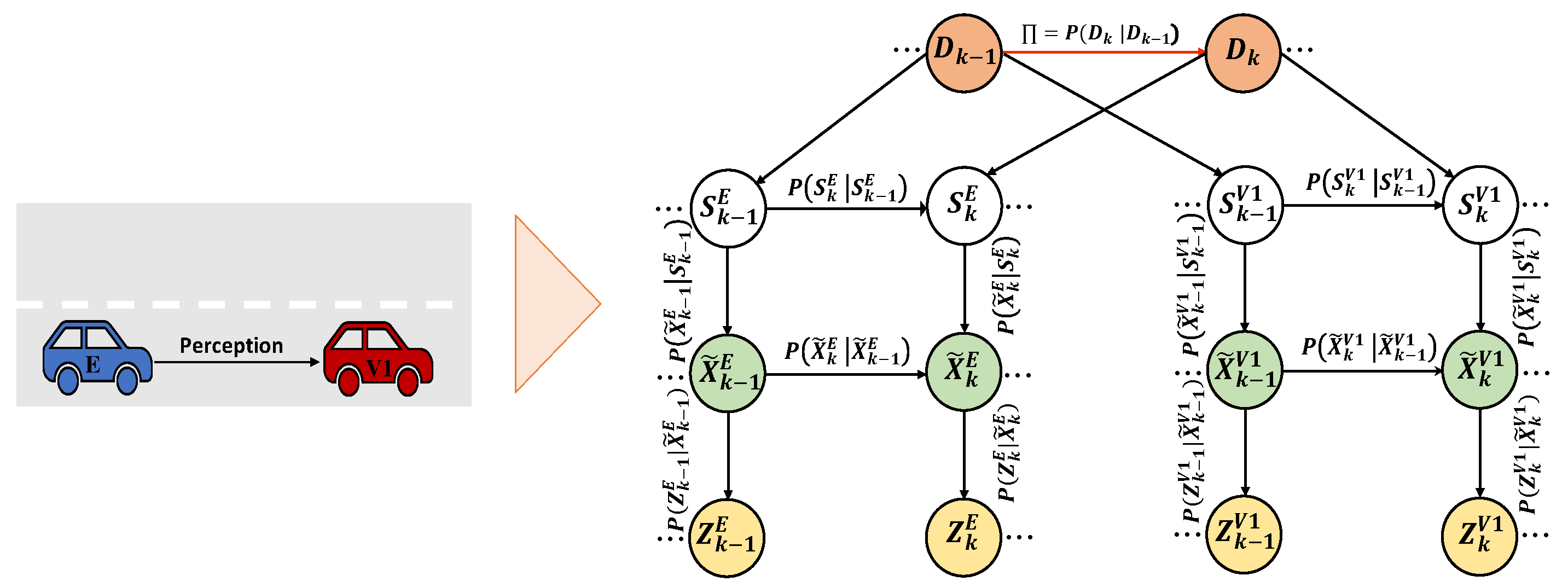
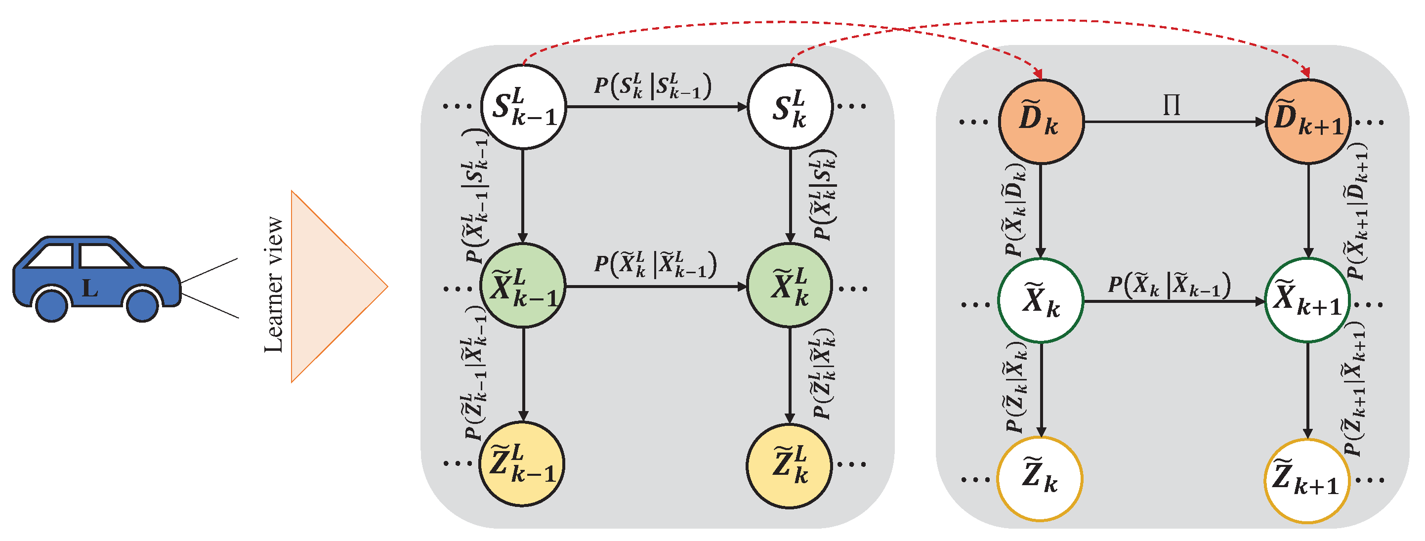
$L$ often relies on observations, formulated as $P ({\tilde{Z}}_{k} | {\tilde{X}}_{k})$ , to deduce actual environmental states that are not directly perceived.
$L$ forms beliefs about the hidden environmental states, represented as ( ${\tilde{D}}_{k}$ , ${\tilde{X}}_{k}$ ). These beliefs evolve according to $P ({\tilde{X}}_{k} | {\tilde{X}}_{k - 1}, {\tilde{D}}_{k})$ and $P ({\tilde{D}}_{k} | {\tilde{D}}_{k - 1}, a_{k - 1})$ .
$L$ engages with its surroundings by choosing actions that minimize the abnormalities and prediction errors.

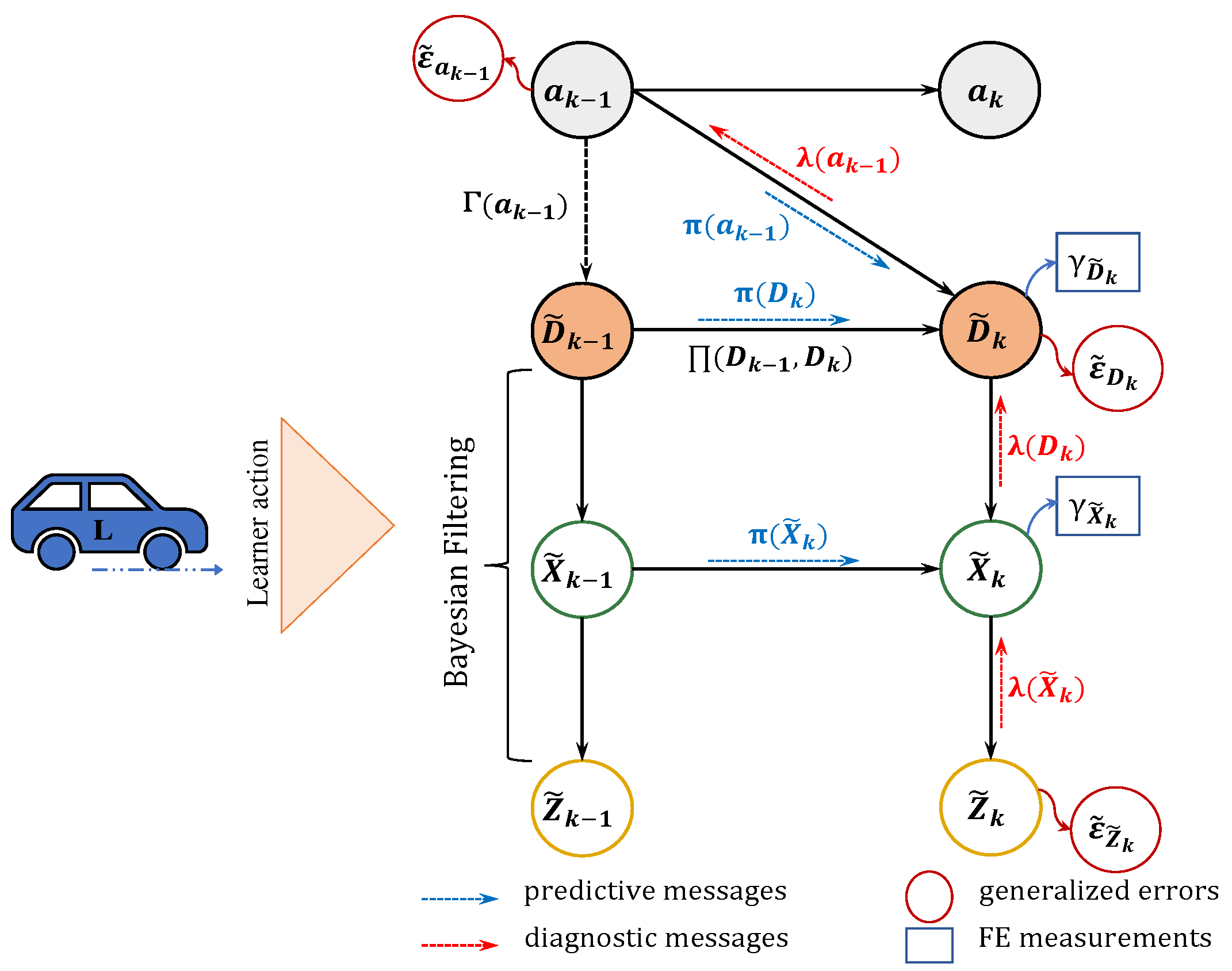
Joint Prediction and Perception:

In the initial stage of the process (at

k = 1

L

employs prior probability distributions, denoted as

P ({\tilde{D}}_{0})

and

P ({\tilde{X}}_{0})

, to predict environmental states. This prediction is realized through the expressions

{\tilde{D}}_{0} \sim P ({\tilde{D}}_{0})

and

{\tilde{X}}_{0} \sim P ({\tilde{X}}_{0})

. The methodological framework for the prediction is grounded in a sophisticated hybrid Bayesian filter, specifically the modified Markov jump particle filter (M-MJPF) [39], which integrates the functionalities of both particle filter (PF) and Kalman filter (KF). As the process progresses beyond the initial stage (for

k > 1

L

leverages the previously accumulated knowledge about the evolution of configurations. This knowledge is encapsulated in the probability distribution

P ({\tilde{D}}_{k} | {\tilde{D}}_{k - 1})

, which is encoded in the transition matrix as outlined in (2). The PF mechanism propagates N particles, each assigned equal weight and derived from the importance density distribution

π ({\tilde{D}}_{k}) = P ({\tilde{D}}_{k} | {\tilde{D}}_{k - 1}, a_{k - 1})

. This process results in the formation of a particle set, represented as

{\{{\tilde{D}}_{k}^{(i)}, w_{k}^{(i)}\}}_{i = 1}^{N}

. Concurrently, a series of Kalman Filters (KFs) is utilized for each particle in the set, facilitating the prediction of the corresponding continuous GSs, denoted as

{\{{\tilde{X}}_{k}^{(i)}\}}_{i = 1}^{N}

. The prediction of these GSs is directed by a higher-level, as indicated in Equation (4), which can be articulated in probabilistic terms as

P ({\tilde{X}}_{k}^{(i)} | {\tilde{X}}_{k - 1}^{(i)}, {\tilde{D}}_{k}^{(i)})

. The posterior distribution associated with these predicted GSs is characterized by the following description:

π ({\tilde{X}}_{k}^{(i)}) = P ({\tilde{X}}_{k}^{(i)}, {\tilde{D}}_{k}^{(i)} | {\tilde{Z}}_{k - 1}) = \int P ({\tilde{X}}_{k}^{(i)} | {\tilde{X}}_{k - 1}^{(i)}, {\tilde{D}}_{k}^{(i)}) λ ({\tilde{X}}_{k - 1}^{(i)}) d {\tilde{X}}_{k - 1}^{(i)},

(7)

where

λ ({\tilde{X}}_{k - 1}^{(i)}) = P ({\tilde{Z}}_{k - 1} | {\tilde{X}}_{k - 1}^{(i)})

represents the diagnostic message that has been previously propagated, following the observation of

{\tilde{Z}}_{k - 1}

at time

k - 1

. This mechanism plays a crucial role in the algorithm’s process: upon receiving a new observation

{\tilde{Z}}_{k}

, a series of diagnostic messages are propagated in a bottom-up manner to update the

L

’s belief about the hidden states. Consequently, the updated belief in the GSs is expressed as

P ({\tilde{X}}_{k}^{(i)}, {\tilde{D}}_{k}^{(i)} | {\tilde{Z}}_{k}) = π ({\tilde{X}}_{k}^{(i)}) \times λ ({\tilde{X}}_{k}^{(i)})

. In parallel, the belief in the discrete hidden states is refined by adjusting the weights of the particles, as denoted by

w_{k}^{(i)} = w_{k}^{(i)} \times λ ({\tilde{D}}_{k})

, where

λ ({\tilde{D}}_{k})

is defined as a discrete probability distribution.

λ ({\tilde{D}}_{k}) = [\frac{\frac{1}{λ ({\tilde{D}}_{k}^{(1)})}}{\frac{1}{\sum_{i = 1}^{m} λ ({\tilde{D}}_{k}^{(i)})}}, \frac{\frac{1}{λ ({\tilde{D}}_{k}^{(2)})}}{\frac{1}{\sum_{i = 1}^{m} λ ({\tilde{D}}_{k}^{(i)})}}, \dots, \frac{\frac{1}{λ ({\tilde{D}}_{k}^{(m)})}}{\frac{1}{\sum_{i = 1}^{m} λ ({\tilde{D}}_{k}^{(i)})}}],

(8)

such that,

\begin{array}{l} λ ({\tilde{D}}_{k}^{(i)}) = λ ({\tilde{X}}_{k}^{(i)}) P ({\tilde{X}}_{k}^{(i)} | {\tilde{D}}_{k}^{(i)}) = 𝓓_{B} (λ ({\tilde{X}}_{k}^{(i)}), P ({\tilde{X}}_{k}^{(i)} | {\tilde{D}}_{k}^{(i)})) = \\ - ln \int \sqrt{λ ({\tilde{X}}_{k}^{(i)}), P ({\tilde{X}}_{k}^{(i)} | {\tilde{D}}_{k}^{(i)})} d {\tilde{X}}_{k}^{(i)}, \end{array}

(9)

where

𝓓_{B}

denotes the Bhattacharyya distance, a measure used to quantify the similarity between two probability distributions. The probability distribution

P ({\tilde{X}}_{k} | {\tilde{D}}_{k})

is assumed to follow a Gaussian distribution

(N)

. This Gaussian distribution is characterized by a mean vector and a covariance matrix as

N (μ_{{\tilde{D}}_{k}}, Σ_{{\tilde{D}}_{k}})

Action Selection:

The decision-making process of

L

hinges on its ability to decide between exploration and exploitation, depends on its interaction with the external environment. This discernment is predicated on the detection of observation anomalies. Specifically,

L

assesses its current state by analyzing the nature of its interactions. In scenarios where the observations align with familiar or normal patterns,

L

solely observes

V 1

. Conversely, in instances characterized by novel or abnormal observations,

L

encounters a more complex situation involving multiple agents (e.g., two dynamic agents

V 1

and

V 2

). This latter scenario represents a deviation from the experiences encapsulated in the expert demonstrations (see Figure 5 and Figure 6). Consequently, based on this assessment,

L

opts for action

a_{k}

, which is informed by its interpretation of environmental awareness and the perceived need for exploration or exploitation according to:

a_{k} = \{\begin{matrix} \underset{a_{k} \in A}{argmax} P (a_{k} | {\tilde{D}}_{k}^{(β)}), if observation is normal then exploit ., \\ q (a_{k - 1}, d_{k}), if observation is abnormal then explore . . \end{matrix}

(10)

In (10), under normal observation,

L

will imitate

E

’s action selected from the active inference table

Γ

defined as:

Γ = [\begin{matrix} P (a_{1} | {\tilde{D}}_{1}), & P (a_{2} | {\tilde{D}}_{1}), & \dots, & P (a_{m} | {\tilde{D}}_{1}) \\ ⋮ & ⋮ & ⋱ & ⋮ \\ P (a_{1} | {\tilde{D}}_{m}), & P (a_{2} | {\tilde{D}}_{m}), & \dots, & P (a_{m} | {\tilde{D}}_{m}) \end{matrix}]

(11)

where

\sum_{i = 1}^{m} P (a_{i} | {\tilde{D}}_{k}) = 1

\forall k

P (a_{i} | {\tilde{D}}_{j}) = \frac{1}{m}

is the probability of selecting action

a_{i} \in A

conditioned to be in configuration

{\tilde{D}}_{j} \in 𝓓

A = {{\dot{μ}}_{{\tilde{D}}_{1}}, {\dot{μ}}_{{\tilde{D}}_{2}}, \dots, {\dot{μ}}_{{\tilde{D}}_{m}}}

is the set of available actions. In addition,

β

denotes the index of the particle with the maximum weight given by:

β = \underset{i}{argmax} {w_{k}^{(i)}}_{i = 1}^{N} .

(12)

In (10), if

L

encounters a situation that is abnormal and hasn’t been seen by

E

before, then

L

will look for new ways to act. It does this by calculating the Euclidean distance

(d_{k})

, which is the shortest distance, between itself and

V 1

when they are in the same lane. Based on the measured distance,

L

adjusts its speed to ensure it doesn’t exceed the speed of

V 1

, helping to prevent a collision (like slowing down or braking).

Free Energy Measurements and GEs

The predictive messages,

π ({\tilde{D}}_{k})

and

π ({\tilde{X}}_{k}^{(i)})

), propagated top-down the hierarchy. At the same time, the AFP-M receives sensory responses in the form of diagnostic messages,

λ ({\tilde{X}}_{k}^{(i)})

and

λ ({\tilde{D}}_{k})

, that move from the bottom level up of the hierarchy. Calculating multi-level Free Energy (FE) helps to understand how well the current observations match what the model predicts.

At the discrete level, FE is measured as the distinction between two types of messages,

π (\tilde{D} k)

and

λ (\tilde{D} k)

, as they enter the node

\tilde{D} k

. These messages are in the form of discrete probability distributions. Therefore, we propose using Kullback-Leibler Divergence (

𝓓 K L

) [40] as a method to measure the probability distance and calculate the difference between these distributions.

Y_{{\tilde{D}}_{k}} = 𝓓_{KL} (π ({\tilde{D}}_{k}), λ ({\tilde{D}}_{k})) + 𝓓_{KL} (λ ({\tilde{D}}_{k}), π ({\tilde{D}}_{k})),

(13)

At the continuous level, FE is conceptualized as the distance between different probabilistic messages arriving at node

\tilde{X} k

. This involves the Bhattacharyya distance between the messages

Y (\tilde{X} k^{(i)})

and

λ ({\tilde{X}}_{k}^{(i)})

, originating from the observation level, that is defined as follows:

Υ_{{\tilde{X}}_{k}^{(i)}} = - l n (BC (π ({\tilde{X}}_{k}^{(i)}), λ ({\tilde{X}}_{k}^{(i)}))),

(14)

where

BC

is the Bhattacharyya coefficient.

Furthermore, Generalized Errors (GEs) facilitate understanding of how to suppress such abnormalities in the future. The GE associated with (13) and conditioned upon transitioning from

{\tilde{D}}_{k - 1}

is defined as:

{\tilde{𝓔}}_{{\tilde{D}}_{k}} = [{\tilde{D}}_{k}, P ({\dot{𝓔}}_{{\tilde{D}}_{k}})] = [{\tilde{D}}_{k}, λ ({\tilde{D}}_{k}) - π ({\tilde{D}}_{k})],

(15)

where

\dot{𝓔} \tilde{D} k

represents an aleatory variable characterized by a discrete probability density function (pdf), denoted as

P (\dot{𝓔} \tilde{D} k)

. The errors identified at the discrete level are then conveyed to the observation level. This process is essential for computing the generalized error at this level, represented as

(\tilde{𝓔} \tilde{Z} k)

, which explains the emergence of a new interaction within the surroundings.

Incremental Active Learning

By integrating the principles of adaptive learning and active inference, our objective is to minimize the occurrence of abnormalities. This goal can be achieved either by constructing a robust and reliable WM or by actively adapting to the dynamics of the environment. Such an approach ensures a comprehensive understanding and interaction with environmental variables, thereby enhancing the system’s predictive accuracy and responsiveness. The information acquired in the previous phases will be utilized to modify the beliefs of

L

and to incrementally expand its knowledge regarding the environment. This process involves updating the active inference table

(Γ)

and expanding the transition matrix

(Π)

. These updates also will take into account the parameter of abnormality observation for considering the similarity between the two configurations.

In situations involving abnormalities,

L

incrementally encodes the novel experiences in WM by updating both the active inference matrix and the transition matrix. It’s important to note that during such abnormal situations,

L

may encounter scenarios that involve configurations not previously experienced. These configurations are characterized by new relative distances between

L

and other dynamic objects in its environment, differing from those configurations previously known by the entity

E

. The discovery and understanding of these new configurations enable

L

to learn and adapt, thereby enhancing its ability to respond to similar situations in the future.

Consequently, a set

𝓒

consisting of the relative distance-action pair can be performed during the abnormal period T (i.e., exploration) as

𝓒 = {{\tilde{Z}}_{k}, a_{k}}_{t}^{T}

can be defined as

𝓓^{'} = {D_{m + 1}, D_{m + 2}, \dots, D_{m + n}} = {D_{1}^{'}, D_{2}^{'}, \dots, D_{n}^{'}}

, where n is the total number of the newly acquired configurations and

D_{l}^{'} \sim N (μ_{D_{l}^{'}}, Σ_{D_{l}^{'}})

such that

D_{l}^{'} \in 𝓓^{'}

. Therefore, the newly experienced action-configuration pairs characterized by

P (a_{k}^{'} | D_{1}^{'})

are encoded in

Γ^{'}

according to:

Γ^{'} = [\begin{matrix} P (a_{1}^{'} | D_{1}^{'}), & P (a_{2}^{'} | D_{1}^{'}), & \dots, & P (a_{n}^{'} | D_{1}^{'}) \\ ⋮ & ⋮ & ⋱ & ⋮ \\ P (a_{1}^{'} | D_{n}^{'}), & P (a_{2}^{'} | D_{n}^{'}), & \dots, & P (a_{n}^{'} | D_{n}^{'}) \end{matrix}],

(16)

Similarly, by analyzing the dynamic evolution of these new configurations, it becomes possible to estimate their transition probabilities

P ({\tilde{D}}_{t} | {\tilde{D}}_{t - 1})

encoded in

Π^{'}

, which is defined as:

Π^{'} = [\begin{matrix} P (D_{1}^{'} | D_{1}^{'}), & \dots, & P (D_{1}^{'} | D_{n}^{'}) \\ ⋮ & ⋱ & ⋮ \\ P (D_{n}^{'} | D_{1}^{'}), & \dots, & P (D_{n}^{'} | D_{n}^{'}) \end{matrix}],

(17)

where

\sum_{k = 1}^{m} P (D_{i}^{'} | D_{k}^{'}) = 1

\forall i

. Consequently, the updated global transition matrix

Π^{″} \in R^{(m + n), (m + n)}

is expressed as:

Π^{″} = [\begin{matrix} Π & 0_{m, n} \\ 0_{n, m} & Π^{'} \end{matrix}],

(18)

where

Π

is the original transition matrix and

Π^{'}

is the newly acquired one.

Action Update:

L

evaluates performed action at time

k - 1

using the FE calculated at time k, as defined in (13) and (14). In abnormal conditions,

L

learns future behaviors by gathering information about its surrounding environment.

During the online learning procedure,

L

modifies/updates the current active inference table and transition matrix, which is based on diagnostic messages, represented by

λ (\tilde{D} k)

and

λ (a_{k - 1})

. Additionally, the transition matrix is refined using the GE defined in (15) as below:

π^{*} ({\tilde{D}}_{k}) = π ({\tilde{D}}_{k}) + P ({\dot{𝓔}}_{{\tilde{D}}_{k}}) .

(19)

The active inference table

Γ

can be adjusted according to:

π^{*} (a_{k}) = π (a_{k}) + P ({\dot{𝓔}}_{a_{k}}),

(20)

where,

π (a_{k}) = P (\cdot | \tilde{D} k)

represents a specific row within

Γ

. Furthermore,

P (\dot{𝓔} a_{k})

denotes the pdf of the GE associated with the active states, which can be calculated as the following:

𝓔_{a_{k - 1}} = [a_{k - 1}, P ({\dot{𝓔}}_{a_{k - 1}})] = [a_{k - 1}, λ (a_{k - 1}) - π (a_{k - 1})],

(21)

where

λ (a_{k - 1}) = λ ({\tilde{D}}_{k}) \times P ({\tilde{D}}_{k} | a_{k - 1})

4. Resuts

In this section, we evaluate the proposed framework across different settings. First, we introduce the experimental dataset. Then, we describe the learning process, encompassing both offline and online phases.

4.1. Experimental Dataset

The dataset used in this study was gathered from real experiments conducted on a university campus, involving various maneuvering scenarios with two Intelligent Campus Automobile (iCab) vehicles [41]. During these experiments, expert demonstrations were recorded. These involved two autonomous vehicles (AVs), iCab1 and iCab2, interacting to execute a specific driving maneuver: iCab2, acting as the expert vehicle (

E

), overtakes iCab1, which represents a dynamic object (

V 1

), from the left side (see Figure 7). Each AV, denoted as (i), was equipped with both exteroceptive and proprioceptive sensors. These sensors collected data on odometry trajectories and control parameters to study the interactions between the AVs. The sensory data provided four-dimensional information, including the AVs’ positions in

(x, y)

coordinates and their velocities (

\dot{x}

\dot{y}

4.2. Offline Learning Phase

The expert demonstrations from the interactions between the two autonomous vehicles, iCab1 and iCab2, are utilized to learn the Situation Model (SM) offline. The learned SM comprises 24 joint clusters that encode the dynamic interaction between the AVs and the corresponding transition matrix, as depicted in Figure 8. Following this, the FP-M is initialized with these 24 learned configurations, which include position data and control parameters, as detailed in Section 3.2.1.

4.3. Online Learning Phase

The offline-acquired FP-M is enhanced with the action node to shape the AFP-M, as discussed in Section 3.2.2. This model enables the learner agent (

L

) to operate in first-person during the online phase. As

L

undertakes a specific driving task, it assesses the situation based on its beliefs about the environmental state’s evolution and actual observations. In normal situations, where observations align with predictions,

L

opts to perform expert-like maneuvers by imitating the expert’s actions, known as exploitation. Conversely, in the face of abnormal conditions, such as encountering an unexpected vehicle,

L

begins to explore new actions based on these novel observations. This approach helps

L

avoid future abnormal situations and successfully achieve its goals. These goals are twofold: avoiding collisions with other vehicles in

L

’s home-lane when overtaking is not feasible due to traffic in the adjacent lane, and when observations are normal,

L

safely overtakes the home-lane vehicle by following the expert’s demonstration.

4.3.1. Action-Oriented Model

Figure 9 illustrates a trajectory performed by

L

in a normal situation, successfully overtaking the home-lane vehicle (

V 1

) by following the prediction.

Conversely, Figure 10 shows how

L

alternates between exploration and exploitation during a driving task when faced with an abnormality, such as encountering a vehicle (

V 2

) in the adjacent lane. In this scenario,

L

deviates from the predicted path to avoid a collision with

V 2

and slows down to maintain a safe distance from

V 1

. This exploratory behavior enables

L

to learn new actions, like braking, in response to the proximity of the two vehicles. As a result,

L

expands its knowledge, adjusts its beliefs, and later applies these novel collected experiences in similar situations. Figure 10 further demonstrates that after learning new observations and actions related to reducing speed,

L

switch to exploitative behavior, using the newly acquired data to maintain a safe distance from

V 1

as long as it observes traffic in the adjacent lane.

Furthermore, Figure 11 depicts how, after navigating the abnormality and with available space in the adjacent lane (as

V 2

is moving faster),

L

once again has the opportunity to overtake

V 1

. These results demonstrate the learned action-oriented model’s effective adaptation to the dynamic variability in the environment.

4.3.2. Cost of Learning

In this section, we explore how updating and expanding the agent’s beliefs about its surroundings minimizes the FE measurement. This minimization occurs through hierarchical processing, where prior expectations generate top-down predictions about likely observations. Any mismatches between these predictions and actual observations are then passed up to higher levels as prediction errors. We examine the efficiency of two action-oriented models in terms of cumulative FE measurement:

Model A, developed in a normal situation during the online learning phase, where $L$ can overtake $V 1$ .
Model B, formulated in an abnormal situation during the online learning phase, where $L$ is temporarily unable to overtake $V 1$ due to traffic in the adjacent lane.

Figure 12 presents the results for Model A, in which

L

undergoes training across 1000 episodes. Additionally, Figure 13 displays the outcomes for Model B, focusing on FE measurements over 2000 training episodes. The increased number of training episodes for Model B is attributed to the more complex experimental scenario it addresses.

5. Conclusions

In this study, we present a comprehensive framework for autonomous vehicle navigation that integrates principles of active inference and incremental learning. Our approach addresses both normal and abnormal driving scenarios, providing a dynamic and adaptive solution for real-world autonomous driving challenges. The proposed framework effectively combines offline learning from expert demonstrations with online adaptive learning. This dual approach allows the autonomous agent to not only replicate expert maneuvers in normal conditions but also to develop novel strategies in response to unobserved environmental changes. Additionally, we introduced an action-oriented model that enables the agent to alternate between exploration and exploitation strategies. This adaptability is crucial in dynamic environments where the agent must constantly balance the need for safety with efficient navigation. In the proposed scenarios involving abnormalities, the learning agent demonstrated an ability to incrementally encode novel experiences and update its beliefs and transition matrix accordingly. This capability ensures that the intelligent agent continuously enhances its understanding of the environment and improves its decision-making process over time. Moreover, the results highlight the effectiveness of the framework in minimizing free energy, indicating a suitable alignment between the agent’s predictions and environmental realities. This alignment is key to the agent’s successful navigation and decision-making abilities. In conclusion, this research contributes significantly to the field of autonomous navigation by presenting an ability to learn from both pre-existing knowledge and ongoing environmental feedback, which is a promising solution for real-world autonomous navigation challenges.

While the current framework shows promising results, future work could focus on scaling the model for more complex environments, such as urban settings crowded with dynamic elements like pedestrians or varied traffic patterns.

Author Contributions

Conceptualization, S.N. and C.R.; methodology, S.N.; software, S.N.; validation, S.N.; formal analysis, S.N., A.K. and C.R.; investigation, S.N.; resources, S.N., and A.K; data curation, S.N.; writing—original draft preparation, S.N.; writing—review and editing, S.N., A.K, L.M., D.G., and C.R.; visualization, S.N, A.K.; supervision, D.G., C.R.; project administration, L.M.; funding acquisition, L.M. All authors have read and agreed to the published version of the manuscript.

Funding

This research received no external funding.

Institutional Review Board Statement

Not applicable.

Informed Consent Statement

Not applicable.

Data Availability Statement

Not applicable.

Conflicts of Interest

The authors declare no conflict of interest.

Abbreviations

The following abbreviations are used in this manuscript:

AD	autonomous driving
ADS	autonomous driving systems
AFP-M	Active First-Person model
AV	autonomous vehicle
E	expert agent
FE	free energy
FP-M	First-Person model
GDBN	Generative Dynamic Bayesian Network
GE	Generalized error
GM	Generative model
GS	Generalized state
IL	imitation learning
KF	Kalman filter
L	learning agent
MJPF	Markov Jump Particle Filter
PF	particle filter
POMDP	partially observed Markov decision process
RL	reinforcement learning
SM	Situation model
WM	World mode

References

Bezai, N.E.; Medjdoub, B.; Al-Habaibeh, A.; Chalal, M.L.; Fadli, F. Future cities and autonomous vehicles: analysis of the barriers to full adoption. Energy and Built Environment 2021, 2, 65–81. [Google Scholar] [CrossRef]
Parekh, D.; Poddar, N.; Rajpurkar, A.; Chahal, M.; Kumar, N.; Joshi, G.P.; Cho, W. A review on autonomous vehicles: Progress, methods and challenges. Electronics 2022, 11, 2162. [Google Scholar] [CrossRef]
Fürnkranz, J.; Gamberger, D.; Lavrač, N. Foundations of rule learning; Springer Science & Business Media, 2012. [Google Scholar]
Goldstein, M.H.; Waterfall, H.R.; Lotem, A.; Halpern, J.Y.; Schwade, J.A.; Onnis, L.; Edelman, S. General cognitive principles for learning structure in time and space. Trends in cognitive sciences 2010, 14, 249–258. [Google Scholar] [CrossRef] [PubMed]
Knill, D.C.; Pouget, A. The Bayesian brain: the role of uncertainty in neural coding and computation. TRENDS in Neurosciences 2004, 27, 712–719. [Google Scholar] [CrossRef] [PubMed]
Gao, X.; Zhang, Z.Y.; Duan, L.M. A quantum machine learning algorithm based on generative models. Science advances 2018, 4, eaat9004. [Google Scholar] [CrossRef]
Krayani, A.; Khan, K.; Marcenaro, L.; Marchese, M.; Regazzoni, C. A Goal-Directed Trajectory Planning Using Active Inference in UAV-Assisted Wireless Networks. Sensors 2023, 23. [Google Scholar] [CrossRef] [PubMed]
Friston, K.; FitzGerald, T.; Rigoli, F.; Schwartenbeck, P.; Pezzulo, G. Active inference: a process theory. Neural computation 2017, 29, 1–49. [Google Scholar] [CrossRef]
Friston, K. The free-energy principle: a unified brain theory? Nature reviews neuroscience 2010, 11, 127–138. [Google Scholar] [CrossRef]
Regazzoni, C.S.; Marcenaro, L.; Campo, D.; Rinner, B. Multisensorial generative and descriptive self-awareness models for autonomous systems. Proceedings of the IEEE 2020, 108, 987–1010. [Google Scholar] [CrossRef]
Ondruš, J.; Kolla, E.; Vertal’, P.; Šarić, Ž. How do autonomous cars work? Transportation Research Procedia 2020, 44, 226–233. [Google Scholar] [CrossRef]
Paden, B.; Čáp, M.; Yong, S.Z.; Yershov, D.; Frazzoli, E. A survey of motion planning and control techniques for self-driving urban vehicles. IEEE Transactions on intelligent vehicles 2016, 1, 33–55. [Google Scholar] [CrossRef]
González, D.; Pérez, J.; Milanés, V.; Nashashibi, F. A review of motion planning techniques for automated vehicles. IEEE Transactions on intelligent transportation systems 2015, 17, 1135–1145. [Google Scholar] [CrossRef]
Pakdamanian, E.; Sheng, S.; Baee, S.; Heo, S.; Kraus, S.; Feng, L. Deeptake: Prediction of driver takeover behavior using multimodal data. In Proceedings of the 2021 CHI Conference on Human Factors in Computing Systems; 2021; pp. 1–14. [Google Scholar]
Wang, Y.; Liu, Z.; Zuo, Z.; Li, Z.; Wang, L.; Luo, X. Trajectory planning and safety assessment of autonomous vehicles based on motion prediction and model predictive control. IEEE Transactions on Vehicular Technology 2019, 68, 8546–8556. [Google Scholar] [CrossRef]
Atkeson, C.G.; Schaal, S. Robot learning from demonstration. ICML, 1997, Vol. 97, pp. 12–20.
Schaal, S. Is imitation learning the route to humanoid robots? Trends in cognitive sciences 1999, 3, 233–242. [Google Scholar] [CrossRef] [PubMed]
Billard, A.; Calinon, S.; Dillmann, R.; Schaal, S. Robot programming by demonstration. In Springer handbook of robotics; Springer, 2008; pp. 1371–1394. [Google Scholar]
Raza, S.; Haider, S.; Williams, M.A. Teaching coordinated strategies to soccer robots via imitation. In Proceedings of the 2012 IEEE International Conference on Robotics and Biomimetics (ROBIO); IEEE, 2012; pp. 1434–1439. [Google Scholar]
Hussein, A.; Gaber, M.M.; Elyan, E.; Jayne, C. Imitation learning: A survey of learning methods. ACM Computing Surveys (CSUR) 2017, 50, 1–35. [Google Scholar] [CrossRef]
Onishi, T.; Motoyoshi, T.; Suga, Y.; Mori, H.; Ogata, T. End-to-end learning method for self-driving cars with trajectory recovery using a path-following function. In Proceedings of the 2019 International Joint Conference on Neural Networks (IJCNN); IEEE, 2019; pp. 1–8. [Google Scholar]
Chen, Z.; Huang, X. End-to-end learning for lane keeping of self-driving cars. In Proceedings of the 2017 IEEE Intelligent Vehicles Symposium (IV); IEEE, 2017; pp. 1856–1860. [Google Scholar]
Bojarski, M.; Del Testa, D.; Dworakowski, D.; Firner, B.; Flepp, B.; Goyal, P.; Jackel, L.D.; Monfort, M.; Muller, U.; Zhang, J.; et al. End to end learning for self-driving cars. arXiv preprint 2016, arXiv:1604.07316. [Google Scholar]
Sauer, A.; Savinov, N.; Geiger, A. Conditional affordance learning for driving in urban environments. In Proceedings of the Conference on Robot Learning. PMLR; 2018; pp. 237–252. [Google Scholar]
Vogt, D.; Ben Amor, H.; Berger, E.; Jung, B. Learning two-person interaction models for responsive synthetic humanoids. Journal of Virtual Reality and Broadcastings 2014, 11. [Google Scholar]
Droniou, A.; Ivaldi, S.; Sigaud, O. Learning a repertoire of actions with deep neural networks. In Proceedings of the 4th International Conference on Development and Learning and on Epigenetic Robotics; IEEE, 2014; pp. 229–234. [Google Scholar]
Liu, M.; Buntine, W.; Haffari, G. Learning how to actively learn: A deep imitation learning approach. In Proceedings of the 56th Annual Meeting of the Association for Computational Linguistics (Volume 1: Long Papers); 2018; pp. 1874–1883. [Google Scholar]
Argall, B.D.; Chernova, S.; Veloso, M.; Browning, B. A survey of robot learning from demonstration. Robotics and autonomous systems 2009, 57, 469–483. [Google Scholar] [CrossRef]
Ross, S.; Bagnell, D. Efficient reductions for imitation learning. In Proceedings of the thirteenth international conference on artificial intelligence and statistics; JMLR Workshop and Conference Proceedings. 2010; pp. 661–668. [Google Scholar]
Gangwani, T.; Peng, J. State-only imitation with transition dynamics mismatch. arXiv preprint 2020, arXiv:2002.11879. [Google Scholar]
Ogishima, R.; Karino, I.; Kuniyoshi, Y. Combining imitation and reinforcement learning with free energy principle 2020.
Kuefler, A.; Morton, J.; Wheeler, T.; Kochenderfer, M. Imitating driver behavior with generative adversarial networks. In Proceedings of the 2017 IEEE Intelligent Vehicles Symposium (IV); IEEE, 2017; pp. 204–211. [Google Scholar]
Schroecker, Y.; Vecerik, M.; Scholz, J. Generative predecessor models for sample-efficient imitation learning. arXiv preprint 2019, arXiv:1904.01139. [Google Scholar]
Yang, Q.; Gu, Y.; Wu, D. Survey of incremental learning. In Proceedings of the 2019 chinese control and decision conference (ccdc); IEEE, 2019; pp. 399–404. [Google Scholar]
Chalup, S.K. Incremental learning in biological and machine learning systems. International Journal of Neural Systems 2002, 12, 447–465. [Google Scholar] [CrossRef]
Kim, S.; Laschi, C.; Trimmer, B. Soft robotics: a bioinspired evolution in robotics. Trends in biotechnology 2013, 31, 287–294. [Google Scholar] [CrossRef]
Nozari, S.; Krayani, A.; Marin, P.; Marcenaro, L.; Martin, D.; Regazzoni, C. Adapting Exploratory Behaviour in Active Inference for Autonomous Driving. In Proceedings of the ICASSP 2023-2023 IEEE International Conference on Acoustics, Speech and Signal Processing (ICASSP); IEEE, 2023; pp. 1–5. [Google Scholar]
Nozari, S.; Krayani, A.; Marin-Plaza, P.; Marcenaro, L.; Gomez, D.M.; Regazzoni, C. Active Inference Integrated With Imitation Learning for Autonomous Driving. IEEE Access 2022, 10, 49738–49756. [Google Scholar] [CrossRef]
Krayani, A.; Alam, A.S.; Marcenaro, L.; Nallanathan, A.; Regazzoni, C. Automatic Jamming Signal Classification in Cognitive UAV Radios. IEEE Transactions on Vehicular Technology 2022, 71, 12972–12988. [Google Scholar] [CrossRef]
Pardo, L. Statistical inference based on divergence measures; CRC press, 2018. [Google Scholar]
Marín-Plaza, P.; et al. Stereo Vision-based Local Occupancy Grid Map for Autonomous Navigation in ROS. In Proceedings of the 11th Joint Conference on Computer Vision, Imaging and Computer Graphics Theory and Applications - Volume 3: VISAPP, (VISIGRAPP 2016). INSTICC; SciTePress, 2016; pp. 701–706. [Google Scholar] [CrossRef]

Figure 1. The proposed cognitive architecture.

Figure 2. Coupled-GDBN representing the dynamic interactions between

E

and

V 1

Figure 2. Coupled-GDBN representing the dynamic interactions between

E

and

V 1

Figure 3. First-Person model consists of a proprioceptive model (right side) and the learned joint configurations (left side) from the learning agent view.

Figure 4. Graphical representation of the Active First-Person model.

Figure 5. Learning agent receives a normal observation. It is allowed to overtake the vehicle directly ahead in its home lane.

Figure 6. The learning agent detects an abnormal situation due to traffic in the adjacent lane, preventing it from overtaking the vehicle ahead.

Figure 7. a) Autonomous vehicles: iCab1 and iCab2. b) An example of an overtaking scenario.

Figure 8. c) Generated clusters and the associated mean actions to them, and d) the generated transition matrix based on AVs movements.

Figure 9. The learner observes a normal interaction, allowing it to follow its predictions.

Figure 10. Confronted with an abnormality, the learner explores new actions in response to these unexpected observations.

Figure 11. After overcoming the abnormality, the learner resumes imitating expert demonstrations.

Figure 12. Cumulative free energy related to Model A. The red curve shows the measurement trend.

Figure 13. Cumulative free energy related to Model B. The red curve shows the measurement trend.

Disclaimer/Publisher’s Note: The statements, opinions and data contained in all publications are solely those of the individual author(s) and contributor(s) and not of MDPI and/or the editor(s). MDPI and/or the editor(s) disclaim responsibility for any injury to people or property resulting from any ideas, methods, instructions or products referred to in the content.

© 2023 by the authors. Licensee MDPI, Basel, Switzerland. This article is an open access article distributed under the terms and conditions of the Creative Commons Attribution (CC BY) license (http://creativecommons.org/licenses/by/4.0/).

Copyright: This open access article is published under a Creative Commons CC BY 4.0 license, which permit the free download, distribution, and reuse, provided that the author and preprint are cited in any reuse.

MDPI Initiatives

Important Links

Choose an area of interest and we will send you notifications of new preprints at your preferred frequency.

Disclaimer

Modeling Autonomous Vehicle Responses to Novel Observations using Hierarchical Cognitive Representations Inspired Active Inference

Abstract

1. Introduction

2. Related Works

3. Proposed Framework

3.1. Perception Module

3.2. Adaptive Learning Module

3.2.1. World Model

3.2.2. Active Model

4. Resuts

4.1. Experimental Dataset

4.2. Offline Learning Phase

4.3. Online Learning Phase

4.3.1. Action-Oriented Model

4.3.2. Cost of Learning

5. Conclusions

Author Contributions

Funding

Institutional Review Board Statement

Informed Consent Statement

Data Availability Statement

Conflicts of Interest

Abbreviations

References

MDPI Initiatives

Important Links

Subscribe