Exploratory Dividend Optimization with Entropy Regularization

1. Introduction

The risk management problem of an insurance company has been studied extensively in the literature. It dates back to the Cramér-Lundberg (C-L) model of Lundberg (1903) which described the surplus process of the insurance company in terms of two cash flows: premiums received and claims paid. Consider an insurance company with claims arriving at Poisson rate $\nu$, i.e., the total number of claims $N_t$ up to time t is Poisson distributed with parameter $\nu t$. Denote by ${\xi }_i$ the size of the i-th claim, where $\left\{{\xi }_i\right\}$’s are independently and identically distributed with $\mathbb{E}\left[{\xi }_i\right]={\mu }_1$ and $\mathbb{E}\left[{\xi }_i^2\right]={\mu }_2$ for some constants ${\mu }_1,{\mu }_2>0$. Let ${\tilde{X}}_t$ denote the surplus process of the insurance company. Then

$$\begin{array}{c}\hfill {\tilde{X}}_t=x_0+\zeta t-\sum _{i=1}^{N_t}{\xi }_i,\end{array}$$

where $x_0$ is the initial surplus level, and $\zeta$ is the premium rate which is the amount of premium received by the insurance company per unit of time.

De Finetti (1957) first proposed the dividend optimization problem: An insurance company maximizes the expectation of cumulative discounted dividends until the ruin time by choosing dividend strategies, that is, when and how much of the surplus should be distributed as dividends to the shareholders. De Finetti (1957) derived that the optimal dividend policy under a simple discrete random walk model should be a barrier strategy. Gerber (1969) then generalized the dividend problem from a discrete-time model to the classical C-L model and showed that the optimal dividend strategy should be band strategy, which degenerates to a barrier strategy for exponentially distributed claim size.

With the development of technical tools such as dynamic programming, the dividend optimization problem has been analyzed under the stochastic control framework. In particular, ${\tilde{X}}_t$ in C-L model can be approximated by a diffusion process $X_t$ that evolves according to

$$\begin{array}{c}\hfill d{X}_t=\mu dt+\sigma d{W}_t,\end{array}$$

where $\mu :=\zeta -\nu {\mu }_1$, $\sigma :=\sqrt{\nu {\mu }_2}$, and $\left\{W_t\right\}$ is a standard Brownian motion; see, e.g., Schmidli (2007). It is worth noting that the diffusion approximation for the surplus process works well for large insurance portfolios, where an individual claim is relatively small compared to the size of the surplus. Under the drifted Brownian motion model the optimal dividend strategy is a barrier strategy, and if the dividend rate is further upper bounded, the optimal dividend strategy is threshold-type; see, e.g., Jeanblanc-Picqué and Shiryaev (1995) and Asmussen and Taksar (1997). Other extensions on the dividend optimization problem include Jgaard and Taksar (1999), Asmussen et al. (2000), Azcue and Muler (2005), Azcue and Muler (2010), Gaier et al. (2003), Kulenko and Schmidli (2008), Yang and Zhang (2005), Choulli et al. (2003), Gerber and Shiu (2006), Avram et al. (2007) and Yin and Wen (2013), etc.

Previous literature studied the dividend optimization problem based on the complete information of the environment, i.e., all the model parameter values are known. This assumption is no longer valid if the environment is a black-box or the model parameter values are unknown. One way to handle this issue is to use the past information to estimate the model parameters and then solve the problem with the estimated parameters. However, the optimal strategy in the classical dividend optimization problem is a barrier-type or threshold-type, which is extremely sensitive to the model parameter values; a slight change in the model parameters would lead to a totally different strategy.1

In contrast to the traditional approach that separates the estimation and optimization, reinforcement learning aims to learn the optimal strategy through trial-and-error interactions with the unknown environment without estimating the model parameters. In particular, one takes different actions in the unknown territory and receives feedbacks to learn the optimal action and use it to further interact with the environment. In recent years, reinforcement learning had successful applications in many fields such as health-care, autonomous control, natural language processing, and video games; see, e.g., Zhao et al. (2009), Komorowski et al. (2018), Mirowski et al. (2016), Zhu et al. (2017), Radford et al. (2017), Paulus et al. (2017), Mnih et al. (2015), Jaderberg et al. (2019), Silver et al. (2016), Silver et al. (2017). There is no doubt that reinforcement learning has become one of the most popular and fastest-growing fields today.

Exploration and exploitation are the key concepts in reinforcement learning, and they proceed simultaneously. On one hand, exploitation is to utilize the so-far-known information to derive the current optimal strategy which might not be optimal from the long-term view. On the other hand, exploration emphasizes learning from trial-and-error interactions with the environment to improve its knowledge for the sake of long-term benefit. While the optimal strategy of the classical dividend optimization problem is deterministic when the model parameter values are fully known, randomized strategies are considered to encourage exploration of other actions in the unknown environment. Although the exploration causes a cost in the short term, it helps to learn the optimal (or near-optimal) strategy and bring benefit from the long-term point of view.

Obviously, how to balance the trade-off between exploitation and exploration is an important issue. The $\epsilon$-greedy strategy is a frequently used randomized strategy in reinforcement learning. It balances the exploration and exploitation by illustrating that the agent should stick to the current optimal policy most of the time, while the agent could sometimes randomly take other non-optimal actions to explore the environment; see, e.g., Auer et al. (2002). Boltzmann exploration is another randomized strategy extensively studied in RL literature. Instead of assigning constant probabilities to different actions based on current information, Boltzmann exploration uses the Boltzmann distribution to allocate the probability to different actions, where the probability of each action is positively related to its reward. In other words, agent should choose action with higher expected rewards with higher probability; see, e.g., Cesa-Bianchi et al. (2017).

Another way to introduce a randomized strategy is to intentionally include a regularization term to encourage exploration. Entropy is a frequently used criterion in the RL family that measures the level of exploration. The entropy regularization framework directly incorporates entropy as a regularization term into the original objective function to encourage exploration; see, e.g., Todorov (2006), Ziebart et al. (2008), Nachum et al. (2017). In the entropy regularization framework, the weight of exploration is determined by the coefficient imposed on the entropy, which is called the temperature parameter. The larger the temperature parameter, the greater the weight of exploration. A temperature parameter that is too large may result in too much focus on exploring the environment and little effort in exploiting the current information; otherwise, if the temperature parameter is too small, one may stick to the current optimal strategy without the opportunity to explore better solutions. Therefore, careful selections of the temperature parameter is important for designing reinforcement learning algorithms.

While most existing literature in reinforcement learning focus on the Markov decision process, recently Wang et al. (2020) extended the entropy regularization framework to the continuous-time setting. The authors showed that the optimal distributional control is Gaussian distribution in the linear-quadratic stochastic control problem. In the series work, Wang and Zhou (2020) studied continuous-time mean-variance portfolio selection problem under the entropy-regularized RL framework and showed that the precommitted strategies are Gaussian distributions with time-decaying variance. Dai et al. (2023) considered the equilibrium mean-variance problem with log return target and showed that the optimal control is Gaussian distribution with the variance term not necessarily decaying in time.

This paper studies the dividend optimization problem in the entropy regularization framework to encourage the exploration in the unknown environment. We follow the same setting as in Wang et al. (2020) which use Shannon’s differential entropy. The key idea is to use distribution as the control to solve the entropy-regularized dividend optimization problem. Consequently, the optimal dividend policy is a randomization over the possible dividend paying rates. We derive the so-called exploratory HJB and establish the theoretical results to guarantee the existence of the solution. We obtain that the optimal exploratory dividend policy is a truncated exponential distribution whose parameter depends on the surplus level and the temperature parameter. We show that, for suitable choices of the maximal dividend paying rate and the temperature parameter, the value function of the exploratory dividend optimization problem could be significantly different from the value function in the traditional problem. In particular, we classify the value function of the exploratory dividend optimization problem into three cases based on its monotonicity.

Recently, Bai et al. (2023) also study the optimal dividend problem under the continuous time diffusion model. The authors then use a policy improvement argument along with policy evaluation devices to construct approximating sequences of the optimal strategy. The difference is that in their paper the feasible controls are open-loop, while we consider feedback controls only. We show that the value function is decreasing when the maximal dividend paying rate is relatively small compared to the temperature parameter, where in their paper the maximal dividend paying rate is assumed to be larger than one and thus the value function is always increasing.

The rest of the paper is organized as follows. In Section 2, we introduce the formulation of the entropy-regularized dividend optimization problem. In Section 3, we present the exploratory HJB and the theoretical results to solve the exploratory dividend problem. We then discuss the three cases of the value function for the exploratory dividend problem in Section 4. Some numerical examples to show the impact of parameters on the optimal dividend policy and the value function are presented in Section 5. Section 6 concludes.

2. Problem

2.1. The Model

Suppose an insurance company has surplus $X_t$ at time t, with

$$\begin{array}{c}\hfill d{X}_t=\mu dt+\sigma d{W}_t,X_0=x,\end{array}$$

(1)

where $\mu >0$, $\sigma >0$, and ${\left\{W_t\right\}}_{t\ge 0}$ is a standard Brownian motion defined on the filtered probability space $(\mathrm{\Omega },\mathcal{F},{\left\{{\mathcal{F}}_t\right\}}_{t\ge 0},\mathbb{P})$. As remarked by Asmussen and Taksar (1997), such a surplus process (1) can be viewed either as a direct modelling with drifted Brownian motion or as an approximation to the classical compound Poisson model.

A dividend strategy or policy is defined as $\mathbf{a}={\left\{a_t\right\}}_{t\ge 0}$, where $a_t$ is the dividend paying rate at time t, i.e., the cumulative amount of dividends paid from time $t_1$ to time $t_2$ is given by ${\int }_{t_1}^{t_2}{a}_{t}dt$. We consider herein the Markov feedback controls, i.e., $a_t=a\left(X_t\right)$, where $a(·)$ is a function of the surplus level $X_t$. Note that $a_t$ is nonnegative for any t. Further, we assume that $a_t$ is upper bounded by a positive constant M, which is consistent with the assumption made in the literature. We give the formal definition of the admissible dividend policy below.

Definition 1. 

A dividend policy $\mathbf{a}$ is said to be admissible if ${\left\{a_t\right\}}_{t\ge 0}$ is ${\mathcal{F}}_t$-adapted and $a_t\in [0,M]$ for all $t\ge 0$.

Denote by $\mathcal{A}$ the set of admissible dividend policies. For an insurance company whose surplus process evolves according to (1) and pays the dividend according to policy $\mathbf{a}={\left\{a_t\right\}}_{t\ge 0}\in \mathcal{A}$, the controlled surplus process for this insurance company is

$$\begin{array}{c}\hfill d{X}_t^{\mathbf{a}}=(\mu -a_t)dt+\sigma d{W}_t,X_0^{\mathbf{a}}=x.\end{array}$$

(2)

Define the ruin time to be the first time that the surplus level hits zero, i.e.,

$$\begin{array}{c}\hfill {\tau }_x^{\mathbf{a}}:=inf\{t\ge 0:X_t^{\mathbf{a}}\le 0\mid X_0^{\mathbf{a}}=x\}.\end{array}$$

For an insurance company starting with initial surplus $x\in [0,\infty )$, the problem is to find the optimal dividend policy that maximizes the expected value of exponentially discounted dividends to be accumulated until the ruin time, that is,

$$\begin{array}{c}\hfill J_{cl}(x,\mathbf{a}):=\mathbb{E}\left[{\int }_0^{{\tau }_x^{\mathbf{a}}}{e}^{-\rho t}a\left(X_t^{\mathbf{a}}\right)dt\right],\end{array}$$

where $\rho >0$ is the discounting rate. Then the optimal dividend problem is

$$\begin{array}{c}\hfill \underset{\mathbf{a}\in \mathcal{A}}{sup}{J}_{cl}(x,\mathbf{a}).\end{array}$$

(3)

2.2. Classical Optimal Dividend Problem

First, we briefly review the results of solving the dividend optimization problem (3) classically. Let $V_{cl}\left(x\right)$ be the value function of the dividend optimization problem:

$$\begin{array}{c}\hfill V_{cl}\left(x\right):=\underset{\mathbf{a}\in \mathcal{A}}{sup}{J}_{cl}(x,\mathbf{a}).\end{array}$$

Assume that the value function $V_{cl}\left(x\right)$ is twice-continuously differentiable. The standard dynamic programming approach leads to the following Hamilton-Jacobi-Bellman equation,

$$\begin{array}{c}\hfill \rho V_{cl}\left(x\right)=\underset{a\in [0,M]}{sup}\left\{a+(\mu -a)V_{cl}^{\prime }\left(x\right)+\frac{1}{2}{\sigma }^2{V}_{cl}^{\prime \prime }\left(x\right)\right\},\end{array}$$

(4)

with boundary condition $V_{cl}\left(0\right)=0$. It can be easily seen that the optimal dividend paying rate at surplus level x is

$$\begin{array}{c}\hfill a^{*}\left(x\right)=\left\{\begin{array}{cc}0,\hfill & \mathrm{if}{V}_{cl}^{\prime }\left(x\right)>1,\hfill \\ M,\hfill & \mathrm{if}{V}_{cl}^{\prime }\left(x\right)\le 1.\hfill \end{array}\right.\end{array}$$

(5)

Assume that $V_{cl}\left(x\right)$ is a concave function. Then there exists a nonnegative constant $x_b$ such that $V_{cl}^{\prime }\left(x\right)\le 1$ when $x\ge x_b$ and $V_{cl}^{\prime }\left(x\right)>1$ when $0\le x<x_b$. Substitute (5) into (4), then it turns into the following ODEs:

$$\begin{array}{c}\hfill \left\{\begin{array}{cc}\frac{1}{2}{\sigma }^2{V}_{cl}^{\prime \prime }\left(x\right)+\mu V_{cl}^{\prime }\left(x\right)-\rho V_{cl}\left(x\right)=0,\hfill & \mathrm{if}0\le x<x_b,\hfill \\ \frac{1}{2}{\sigma }^2{V}_{cl}^{\prime \prime }\left(x\right)+(\mu -M)V_{cl}^{\prime }\left(x\right)-\rho V_{cl}\left(x\right)+M=0,\hfill & \mathrm{if}x\ge x_b.\hfill \end{array}\right.\end{array}$$

(6)

Combining with the boundary condition, one can derive that

$$\begin{array}{c}\hfill V_{cl}\left(x\right)=\left\{\begin{array}{cc}{C}_1\left(e^{{\theta }_{1}x}-e^{-{\theta }_{2}x}\right),\hfill & \mathrm{if}0\le x<x_b,\hfill \\ \frac{M}{\rho }-C_2{e}^{-{\theta }_{3}x},\hfill & \mathrm{if}x\ge x_b,\hfill \end{array}\right.\end{array}$$

(7)

where

$$\begin{array}{c}\hfill {\theta }_1=\frac{-\mu +\sqrt{{\mu }^2+2\rho {\sigma }^2}}{{\sigma }^2},{\theta }_2=\frac{\mu +\sqrt{{\mu }^2+2\rho {\sigma }^2}}{{\sigma }^2},{\theta }_3=\frac{(\mu -M)+\sqrt{{(\mu -M)}^2+2\rho {\sigma }^2}}{{\sigma }^2}.\end{array}$$

$C_1$, $C_2$ and $x_b$ are determined by the smooth pasting conditions, i.e.,

$$\begin{array}{c}\hfill \left\{\begin{array}{c}{C}_1\left(e^{{\theta }_1{x}_b}-e^{-{\theta }_2{x}_b}\right)=\frac{M}{\rho }-C_2{e}^{-{\theta }_3{x}_b},\hfill \\ C_1\left({\theta }_1{e}^{{\theta }_1{x}_b}+{\theta }_2{e}^{-{\theta }_2{x}_b}\right)=1,\hfill \\ C_2{\theta }_3{e}^{-{\theta }_3{x}_b}=1.\hfill \end{array}\right.\end{array}$$

(8)

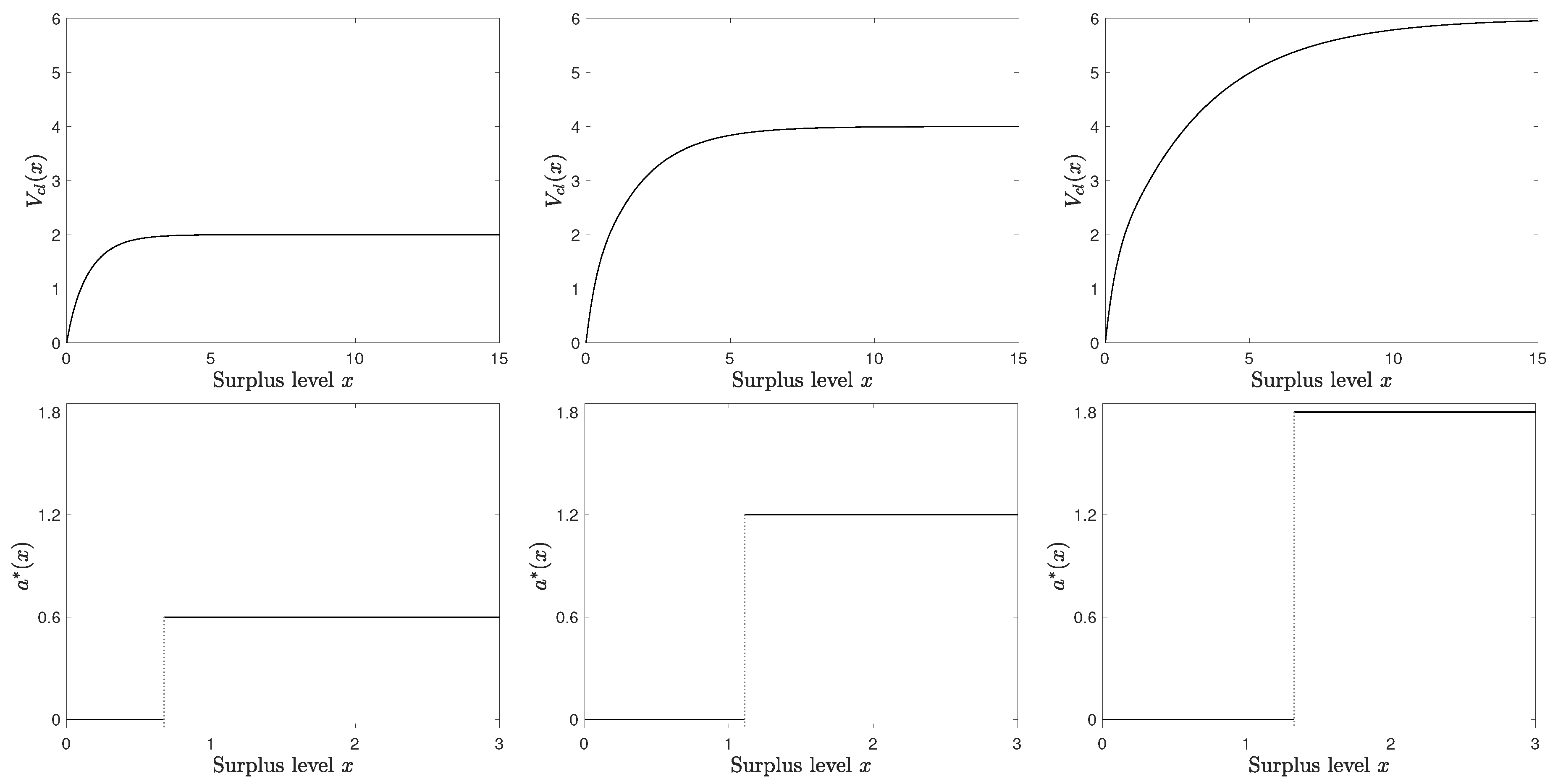
If $\frac{M}{\rho }-\frac{1}{{\theta }_3}>0$, there exists unique solution to (8). In this case, $V_{cl}\left(x\right)$ is given by (7), where $C_1,C_2,x_b$ are determined uniquely through (8). Consequently, the optimal dividend policy is to pay the maximal rate M when surplus level x exceeds threshold $x_b$ and to pay nothing if else. If $\frac{M}{\rho }-\frac{1}{{\theta }_3}\le 0$, then $V_{cl}\left(x\right)=\frac{M}{\rho }(1-e^{-{\theta }_{3}x})$. In this case, the optimal dividend policy is always to pay the maximal rate M. Detailed proofs can be found in Asmussen and Taksar (1997). It is also straightforward to check that the optimal value function $V_{cl}\left(x\right)$ is concave on x and always smaller than $M/\rho$ which is the limit of $V_{cl}\left(x\right)$ as x going to infinity. Figure 1 below illustrates the value function and the corresponding optimal dividend policy under the following parameter values: $\mu =1$, $\sigma =1$, $\rho =0.3$, $M=0.6$ (left panels), $M=1.2$ (middle panels), and $M=1.8$ (right panels), respectively.

2.3. Exploratory Formulation

The above optimal dividend policy (5) is implemented based on the complete information, i.e., the model parameters $\mu$ and $\sigma$ are known. In reality, however, it is difficult to know exactly the values of $\mu$ and $\sigma$, due to the uncertainty in premium rate, claim arrival process and claim size. Therefore, we consider a technique named reinforcement learning to learn the optimal (or near-optimal) dividend paying strategy through trial-and-error interactions with the unknown territory.

Whereas the majority of the work in reinforcement learning consider Markov decision process in discrete time, we follow the pioneering work of Wang et al. (2020) who model the reinforcement learning in continuous time as a relaxed stochastic control problem. At time t with surplus level $X_t$ the dividend paying rate a is randomly sampled according to a distribution ${\pi }_t:=\pi (a;X_t)$, where $\pi (·;·):[0,M]\times [0,\infty )\mapsto [0,\infty )$, satisfying ${\int }_0^M\pi (a;x)da=1$ for any $x\in [0,\infty )$. We call $\pi :={\left\{{\pi }_t\right\}}_{t\ge 0}$ the distributional dividend policy. Following the same procedure as in Wang et al. (2020), we derive the exploratory dynamic of the surplus process under $\pi$ to be

$$\begin{array}{c}\hfill d{X}_t^{\pi }=\left(\mu -{\int }_0^{M}a\pi (a;X_t^{\pi })da\right)dt+\sigma d{W}_t,X_0^{\pi }=x,\end{array}$$

(9)

and the expected value of total discounted dividends under exploration to be

$$\begin{array}{c}\hfill \mathbb{E}\left[{\int }_0^{{\tau }_x^{\pi }}{e}^{-\rho t}{\int }_0^{M}a\pi (a;X_t^{\pi })dadt\right],\end{array}$$

where the ruin time is

$$\begin{array}{c}\hfill {\tau }_x^{\pi }:=inf\{t\ge 0:X_t^{\pi }\le 0\mid X_0^{\pi }=x\}.\end{array}$$

In addition to the expected value of total discounted dividends under exploration, Shannon’s differential entropy is introduced into the objective to encourage exploration. For a given distribution $\pi$, the entropy is defined as

$$\begin{array}{c}\hfill \mathcal{H}\left(\pi \right):=-{\int }_0^M\pi \left(a\right)ln\pi \left(a\right)da.\end{array}$$

(10)

Thus, the objective of entropy-regularized exploratory dividend problem is

$$\begin{array}{cc}\hfill J(x,\pi ):& =\mathbb{E}\left[{\int }_0^{{\tau }_x^{\pi }}{e}^{-\rho t}\left({\int }_0^{M}a\pi (a;X_t^{\pi })da+\lambda \mathcal{H}\left({\pi }_t\right)\right)dt\right]\hfill \\ \hfill & =\mathbb{E}\left[{\int }_0^{{\tau }_x^{\pi }}{e}^{-\rho t}\left({\int }_0^M\left(a-\lambda ln\pi (a;X_t^{\pi })\right)\pi (a;X_t^{\pi })da\right)dt\right],\hfill \end{array}$$

(11)

where $\lambda >0$ is the so-called temperature parameter. Note that $\lambda$ controls the weight to be put on the exploration and is exogenously given. If $\lambda =0$, the distribution degenerates to the Dirac measure, which is the solution to classical optimal dividend problem without exploration. The entropy-regularized exploratory dividend problem is

$$\begin{array}{c}\hfill \underset{\pi \in \Pi }{sup}J(x,\pi ),\end{array}$$

(12)

where $\Pi$ is the set of admissible exploratory dividend policies. We give the formal definition of admissible exploratory dividend policy $\pi$ below.

Definition 2. 

An exploratory dividend policy π is admissible if the following conditions are satisfied:

(i) 

$\pi (·;x)\in {\Pi }_{[0,M]}$ for any $x\in [0,\infty )$, where ${\Pi }_{[0,M]}$ is a set of probability density functions with support $[0,M]$;

(ii) 

the stochastic differential equation (9) has a unique solution ${\left\{X_t^{\pi }\right\}}_{t\ge 0}$ under π;

(iii) 

$\mathbb{E}\left[{\int }_0^{{\tau }_x^{\pi }}{e}^{-\rho t}\left|{\int }_0^M\left(a-\lambda ln\pi (a;X_t^{\pi })\right)\pi (a;X_t^{\pi })da\right|dt\right]<\infty$.

The following proposition will be used later.

Proposition 1. 

For any distribution π on support $[0,M]$, the entropy $\mathcal{H}\left(\pi \right)\le lnM$.

3. Exploratory HJB Equation

To solve exploratory optimal dividend problem (12), we first derive the corresponding HJB equation, the so-called exploratory HJB; see Wang et al. (2020), Tang et al. (2022), etc.

Let $V\left(x\right)$ be the value function of entropy-regularized exploratory dividend problem, that is,

$$\begin{array}{c}\hfill V\left(x\right):=\underset{\pi \in \Pi }{sup}J(x,\pi ).\end{array}$$

Assume that the value function $V\left(x\right)$ is twice-continuously differentiable. Following the standard arguments in dynamic programming, we derive the exploratory HJB equation below:

$$\begin{array}{c}\hfill \rho V\left(x\right)=\underset{\pi \in {\Pi }_{[0,M]}}{sup}\left\{{\int }_0^M\left[a(1-V^{\prime }\left(x\right))-\lambda ln\pi (a;x)\right]\pi (a;x)da\right\}+\mu V^{\prime }\left(x\right)+\frac{1}{2}{\sigma }^2{V}^{\prime \prime }\left(x\right),\end{array}$$

(13)

with boundary condition

$$\begin{array}{c}\hfill V\left(0\right)=0.\end{array}$$

(14)

3.1. Exploratory Dividend Policy

To solve the supremum in (13) together with the constraint that ${\int }_0^M\pi (a;x)da=1$, we introduce the Lagrange multiplier $\eta$:

$$\begin{array}{c}\hfill \underset{\pi \in {\Pi }_{[0,M]}}{sup}\left\{{\int }_0^M\left[a(1-V^{\prime }\left(x\right))-\lambda ln\pi (a;x)-\eta \right]\pi (a;x)da+\eta \right\}.\end{array}$$

Maximizing the integrand above pointwisely and using the first-order condition leads to the solution

$$\begin{array}{c}\hfill {\pi }^{*}(a;x)=exp\left(a\left(\frac{1-V^{\prime }\left(x\right)}{\lambda }\right)-1-\frac{\eta }{\lambda }\right),a\in [0,M].\end{array}$$

Because ${\int }_0^M{\pi }^{*}(a;x)da=1$, we solve that

$$\begin{array}{c}\hfill {\pi }^{*}(a;x)=\frac{1}{Z_M((1-V^{\prime }\left(x\right))/\lambda )}exp\left(a\left(\frac{1-V^{\prime }\left(x\right)}{\lambda }\right)\right),a\in [0,M],\end{array}$$

(15)

where

$$\begin{array}{c}\hfill Z_M\left(y\right):=\left\{\begin{array}{cc}\frac{e^{My}-1}{y},\hfill & y\ne 0\hfill \\ M,\hfill & y=0.\hfill \end{array}\right.\end{array}$$

(16)

Recall that the classical optimal dividend policy given in (5) is two-threshold strategy, i.e., it pays nothing, $a^{*}\left(x\right)=0$, if $V_{cl}^{\prime }\left(x\right)>1$ or pays the maximal rate, $a^{*}\left(x\right)=M$, if $V_{cl}^{\prime }\left(x\right)\le 1$. In contrast, the exploratory dividend policy is not restricted to two extreme actions only but gives the probability to take certain actions. This result is very similar to [38] in which the authors study the temperature control problem for Langevin diffusions by incorporating randomization of the temperature control and regularizing its entropy. The classical optimal control of such a problem is of the bang-bang type, whereas the exploratory control is a state-dependent, truncated exponential distribution. Likewise, the optimal distribution ${\pi }^{*}(a;x)$ given in (15) is also a continuous version of Boltzmann distribution or Gibbs measure which is widely used in discrete reinforcement learning.

When $V^{\prime }\left(x\right)>1$, ${\pi }^{*}(a;x)$ is decreasing in a so it has large probability to take small dividend pay-out rate close to 0; when $V^{\prime }\left(x\right)<1$, ${\pi }^{*}(a;x)$ is increasing in a so it has large probability to take large dividend pay-out rate close to M ; when $V^{\prime }\left(x\right)=1$, it degenerates to a uniform distribution on $[0,M]$. In other words, the optimal exploratory dividend policy is an “exploration” of the classical dividend pay-out policy: it searches around the current optimal dividend rate given by the classical solution, 0 or M, with the probability to take a certain rate decreasing as it moving away from the classical solution.

The exploratory surplus process under the optimal policy is well-posed. Note that the optimal distributional policy is ${\pi }^{*}={\left\{{\pi }_t^{*}\right\}}_{t\ge 0}$, where

$$\begin{array}{c}\hfill {\pi }_t^{*}:={\pi }^{*}(a;X_t^{{\pi }^{*}})=\frac{1}{Z_M((1-V^{\prime }\left(X_t^{{\pi }^{*}}\right))/\lambda )}exp\left(a\left(\frac{1-V^{\prime }\left(X_t^{{\pi }^{*}}\right)}{\lambda }\right)\right).\end{array}$$

(17)

Applying the optimal distributional policy (17) into the exploratory surplus process (9), we obtain that

$$\begin{array}{cc}\hfill d{X}_t^{{\pi }^{*}}& =\left(\mu -{\int }_0^{M}a{\pi }^{*}(a;X_t^{{\pi }^{*}})da\right)dt+\sigma d{W}_t\hfill \\ \hfill & =\left[\mu -\left(M-\frac{\lambda }{1-V^{\prime }\left(X_t^{{\pi }^{*}}\right)}+\frac{M}{e^{M(1-V^{\prime }\left(X_t^{{\pi }^{*}}\right))/\lambda }-1}\right){\mathbf{1}}_{V^{\prime }\left(X_t^{{\pi }^{*}}\right)\ne 1}-\left(\frac{M}{2}\right){\mathbf{1}}_{V^{\prime }\left(X_t^{{\pi }^{*}}\right)=1}\right]dt\hfill \\ \hfill & +\sigma d{W}_t.\hfill \end{array}$$

(18)

Since ${\int }_0^{M}a{\pi }^{*}(a;X_t^{{\pi }^{*}})da\in [0,M]$, the SDE (18) has bounded drift and constant volatility. As a result, there exists unique solution $\left\{X_t^{{\pi }^{*}}\right\}$ to (18).

3.2. Verification Theorem

Substituting the optimal distribution ${\pi }^{*}(a;x)$ as shown in (15) into the HJB equation (13), we have the following equation for $V\left(x\right)$:

$$\begin{array}{c}\hfill \rho V\left(x\right)=\mu V^{\prime }\left(x\right)+\frac{1}{2}{\sigma }^2{V}^{\prime \prime }\left(x\right)+\lambda ln{Z}_M((1-V^{\prime }\left(x\right))/\lambda ),\end{array}$$

or equivalently,

$$\begin{array}{cc}\hfill \rho V\left(x\right)=& \mu V^{\prime }\left(x\right)+\frac{1}{2}{\sigma }^2{V}^{\prime \prime }\left(x\right)\hfill \\ \hfill & +\lambda ln\left(\frac{\lambda }{1-V^{\prime }\left(x\right)}\left(e^{M(1-V^{\prime }\left(x\right))/\lambda }-1\right){\mathbf{1}}_{V^{\prime }\left(x\right)\ne 1}+M{\mathbf{1}}_{V^{\prime }\left(x\right)=1}\right).\hfill \end{array}$$

(19)

The following verification theorem shows that $V\left(x\right)$ that solves (19) is indeed the value function of the exploratory dividend problem (12).

Theorem 1. 

Assume there exists twice-continuously differentiable function V that solves (19) with boundary condition (14), and $\left|V\right|,|V^{\prime }|$ are bounded. Then V is the value function of entropy-regularized exploratory dividend problem (12) under exponential discounting.

Theorem 1 shows that solution to the exploratory HJB equation (19) could be the value function of exploratory dividend problem (12). On the other hand, a similar argument could show that the value function shall also satisfy (19), while the optimal exploratory dividend strategy is given by (17). To establish a rigorous statement, we need the following result. The next proposition shows that the value function $V\left(x\right)$ converges as x going to infinity.

Proposition 2. 

Let V be the value function of (12) and suppose the optimal exploratory dividend strategy is (17). Then as x going to infinity, $V\left(x\right)$ converges to a constant, i.e.,

$$\begin{array}{c}\hfill \underset{x\to \infty }{lim}V\left(x\right)=\frac{\lambda ln\lambda +\lambda ln(e^{M/\lambda }-1)}{\rho }.\end{array}$$

(20)

3.3. Solution to Exploratory HJB

Compared with the differential equation (6) which solves the classical value function, the exploratory HJB equation (19) has a nonlinear term $ln{Z}_M((1-V^{\prime }\left(x\right))/\lambda )$, which makes it difficult to be solved explicitly. The theorem below guarantees the existence and uniqueness of solution $V\left(x\right)$.

Theorem 2. 

There exists a unique twice-continuously differentiable function $V\left(x\right)$ that solves (19) with boundary condition (14) and (20). Moreover, ${lim}_{\lambda \to 0}|V\left(x\right)-V_{cl}\left(x\right)|=0$ for all $x\in [0,\infty )$, where $V_{cl}\left(x\right)$ is the value function of classical dividend problem.

Theorem 2 follows from the results in Tang et al. (2022, Theorem 3.9, 3.10) and in Strulovici and Szydlowski (2015, Proposition 1). It is straightforward to check that the conditions to guarantee the existence and uniqueness of the solution to (19) and its twice-continuous differentiability are satisfied.

Theorem 2 also states that when $\lambda$ becomes smaller, the exploratory value function converges to the classical value function. Indeed, a stronger convergence is established by Tang et al. (2022) that V converges to $V_{cl}$ locally uniformly as $\lambda$ going to 0. Note that the parameter $\lambda$ is the weight to be put on the exploration in contrast to the exploitation. If it is more close to 0, the entropy term has smaller effect on the total objective value and the optimal exploratory distribution ${\pi }^{*}(a;x)$ in (15) are more concentrated and close to the Dirac distribution – the optimal solution to the classical dividend optimization problem. Then not surprisingly, the exploratory value function $V\left(x\right)$ also converges to the classical value function $V_{cl}\left(x\right)$ as $\lambda$ going to 0.

Now, thanks to Theorem 2, we have $V\left(x\right)$ that solves the exploratory HJB equation (19). On the other hand, it is straightforward to show that according to (20), if $M<\lambda ln\left(1/\lambda +1\right)$, the limit of $V\left(x\right)$ is negative; if $M>\lambda ln\left(1/\lambda +1\right)$, the limit of $V\left(x\right)$ is positive; if $M=\lambda ln\left(1/\lambda +1\right)$, the limit of $V\left(x\right)$ is zero. The next theorem shows that indeed, we classify $V\left(x\right)$ into three cases based on its monotonicity.

Theorem 3. 

Let $V\left(x\right)$ be the solution to (19) with boundary condition (14) and (20). Then $V\left(x\right)$ is monotone. To be more specific,

(i) 

if $M<\lambda ln\left(1/\lambda +1\right)$, $V\left(x\right)$ is non-increasing.

(ii) 

if $M>\lambda ln\left(1/\lambda +1\right)$, $V\left(x\right)$ is non-decreasing.

(iii) 

if $M=\lambda ln\left(1/\lambda +1\right)$, $V\left(x\right)\equiv 0$.

The following corollary is a direct result from above theorem.

Corollary 1. 

Let $V\left(x\right)$ be the solution to (19) with boundary condition (14) and (20). Then $\left|V\right(x\left)\right|$ and $|V^{\prime }\left(x\right)|$ are bounded.

Note that in Theorem 1 we need $\left|V\right|$ and $|V^{\prime }|$ to be bounded so that V – solution to (19) – is indeed the value function of exploratory optimal dividend problem. Corollary 1 verifies the boundedness conditions are satisfied. In other words, the solution to the exploratory HJB equation (19) is the value function of the exploratory dividend problem.

4. Discussion

In view of Theorem 3, value functions can be classified into three cases according to the monotonicity: (1) $M<\lambda ln\left(1/\lambda +1\right)$; (2) $M>\lambda ln\left(1/\lambda +1\right)$; (3) $M=\lambda ln\left(1/\lambda +1\right)$. The following proposition will be useful in analyzing the properties of value functions.

Proposition 3. 

(a) Define

$$\begin{array}{c}\hfill d_1\left(\lambda \right):=\lambda ln\left(1/\lambda +1\right){\mathbf{1}}_{\lambda >0}+0·{\mathbf{1}}_{\lambda =0},\lambda \in [0,\infty ).\end{array}$$

Then $d_1\left(\lambda \right)$ is increasing. Therefore, ${lim}_{\lambda \to 0}{d}_1\left(\lambda \right)=d_1\left(0\right)=0$ and ${lim}_{\lambda \to \infty }{d}_1\left(\lambda \right)=1$;

• (b) Define

  $$\begin{array}{c}\hfill d_2\left(\lambda \right):=\lambda ln\left(\lambda /\left(\lambda -1\right)\right){\mathbf{1}}_{\lambda >1}+\infty ·{\mathbf{1}}_{\lambda \in [0,1]},\lambda \in [0,\infty ).\end{array}$$
  Then $d_2\left(\lambda \right)>d_1\left(\lambda \right)$, and $d_2\left(\lambda \right)$ is decreasing on $\lambda >1$. Therefore, ${lim}_{\lambda \to 1}{d}_2\left(\lambda \right)=\infty$ and ${lim}_{\lambda \to \infty }{d}_2\left(\lambda \right)=1$.

Case 1: $M<d_1\left(\lambda \right)$.

The value function in this case is non-increasing and thus non-positive, as a sharp contrast to the results of classical dividend problem. To see the reason, on one hand, note that for $\lambda >0$,

$$\begin{array}{c}\hfill lnM<ln{d}_1\left(\lambda \right)=ln\left(\lambda ln\left(\frac{1}{\lambda }+1\right)\right)\le ln\left(\lambda ·\frac{1}{\lambda }\right)=0.\end{array}$$

Then due to Proposition 1, the entropy term is negative, that is, $\mathcal{H}\left(\pi \right)\le lnM<0$. On the other hand, when $d_1\left(\lambda \right)$ is large, it implies that the exploration parameter $\lambda$ is relatively large compared with the maximal dividend paying rate M. Then the negative entropy has a large weight in the total objective value, dominating the total expected dividends and leading to a negative value function.

Case 2: $M>d_1\left(\lambda \right)$.

When $M>d_1\left(\lambda \right)$, the value function is non-decreasing, which is closer to the increasing value function in classical dividend optimization problem than it does in Case 1. This is because a relatively small $\lambda$ compared with M decreases the weight of entropy term in the total objective value. Note that in classical dividend optimization the limit of value function is $M/\rho$, while in the current exploratory dividend optimization the limit of value function is given in (20). Therefore, if (i) $d_1\left(\lambda \right)<M\le d_2\left(\lambda \right)$, the limit of $V\left(x\right)$ is no larger than that of $V_{cl}\left(x\right)$; if (ii) $d_2\left(\lambda \right)<M$, then $V\left(x\right)$ asymptotically achieves a higher value than that of the classical dividend optimization. Then if $\lambda >1$ and $M>\lambda ln\lambda -\lambda ln(\lambda -1)=d_2\left(\lambda \right)$, the limit of $V\left(x\right)$ is larger than that of $V_{cl}\left(x\right)$.

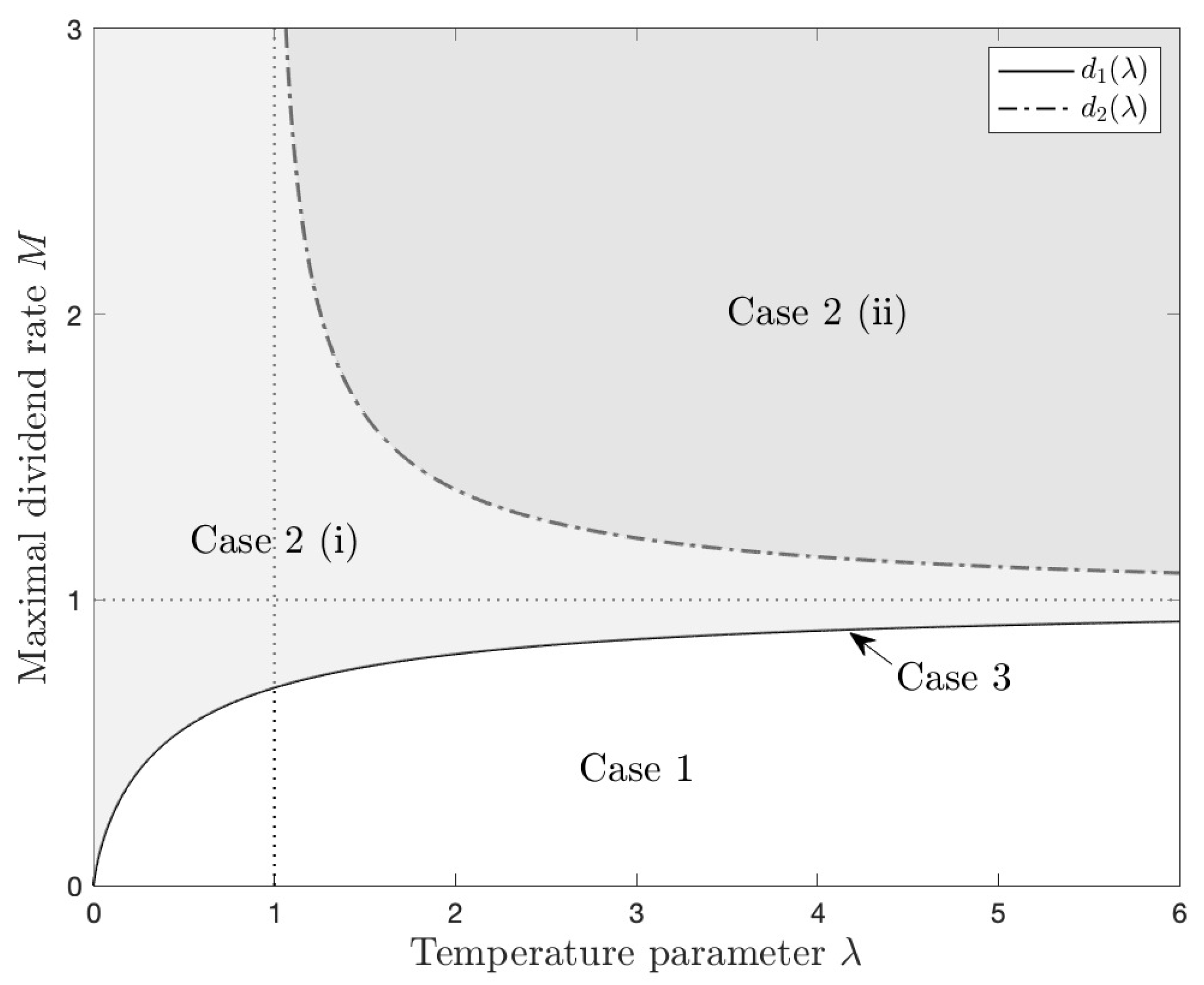
As shown in Proposition 3, for any $\lambda \ge 0$, $d_1\left(\lambda \right)<{lim}_{\lambda \to \infty }{d}_1\left(\lambda \right)=1$. Therefore, when $M\ge 1$, it always belongs to Case 2 for any $\lambda \ge 0$. On the other hand, for any $\lambda \ge 0$, $d_2\left(\lambda \right)>{lim}_{\lambda \to \infty }{d}_2\left(\lambda \right)=1$. Therefore, when $M\le 1$ or $\lambda \le 1$, since $d_2\left(\lambda \right)>M$, it cannot be Case 2 (ii); when $\lambda \le 1$ and $M\ge 1$, it is always Case 2 (i). Note that $\lambda =0$ corresponds to the classical dividend optimization and $d_1\left(0\right)=0$, $d_2\left(0\right)=\infty$ by definition. Since $d_1\left(0\right)<M<d_2\left(0\right)$ for any positive constant M, classical dividend optimization can be viewed as a special Case 2 (i). It implies that exploratory dividend optimization is a generalization of the classical dividend optimization.

Case 3: $M=d_1\left(\lambda \right)$.

As shown in Theorem 3, the value function in this case should be constantly zero. This is because $\lambda$ compared with M happens to strike a balance between exploitation and exploration such that the total expected dividends is offset by the entropy.

Figure 2 depicts the different cases of value functions given different combinations of M and $\lambda$. When $M<d_1\left(\lambda \right)$, the value function falls into Case 1 area. When $M>d_1\left(\lambda \right)$, the value function corresponds to Case 2, which can be further classified into two cases based on the comparison of M and $d_2\left(\lambda \right)$, i.e., whether the value function asymptotically achieves a higher value than that of the classical problem. When $M=d_1\left(\lambda \right)$, the value function should be Case 3 type.

5. Numerical Examples

In this section, we present numerical examples of optimal exploratory policy and corresponding value function which solves exploratory HJB equation (19) based on the theoretical results obtained in the previous sections.2 To have a clear vision on the weight of cumulative dividends and that of entropy in the total objective value, we further decompose $V\left(x\right)$ into two parts: the expected total discounted dividends under the optimal exploratory dividend policy

$$\begin{array}{c}\hfill Dv\left(x\right):=\mathbb{E}\left[{\int }_0^{{\tau }_x^{{\pi }^{*}}}{e}^{-\rho t}\left({\int }_0^{M}a{\pi }^{*}(a;X_t^{{\pi }^{*}})da\right)dt\right];\end{array}$$

and the expected total weighted discounted entropy under the optimal exploratory dividend policy

$$\begin{array}{c}\hfill Entr\left(x\right):=\lambda \mathbb{E}\left[{\int }_0^{{\tau }_x^{{\pi }^{*}}}{e}^{-\rho t}\mathcal{H}\left({\pi }_t^{*}\right)dt\right],\end{array}$$

where the entropy of ${\pi }^{*}$ is derived via substituting the optimal distribution (15) into the definition of entropy (10), i.e.,

$$\begin{array}{c}\hfill \mathcal{H}\left({\pi }^{*}\right)=ln\left(Z_M((1-V^{\prime }\left(x\right))/\lambda )\right)-\frac{M{e}^{M(1-V^{\prime }\left(x\right))/\lambda }}{Z_M((1-V^{\prime }\left(x\right))/\lambda )}+1.\end{array}$$

(21)

Hence, $V\left(x\right)=Dv\left(x\right)+Entr\left(x\right)$. We show examples of three cases, respectively, with commonly used parameters: $\mu =1$, $\sigma =1$, $\rho =0.3$.

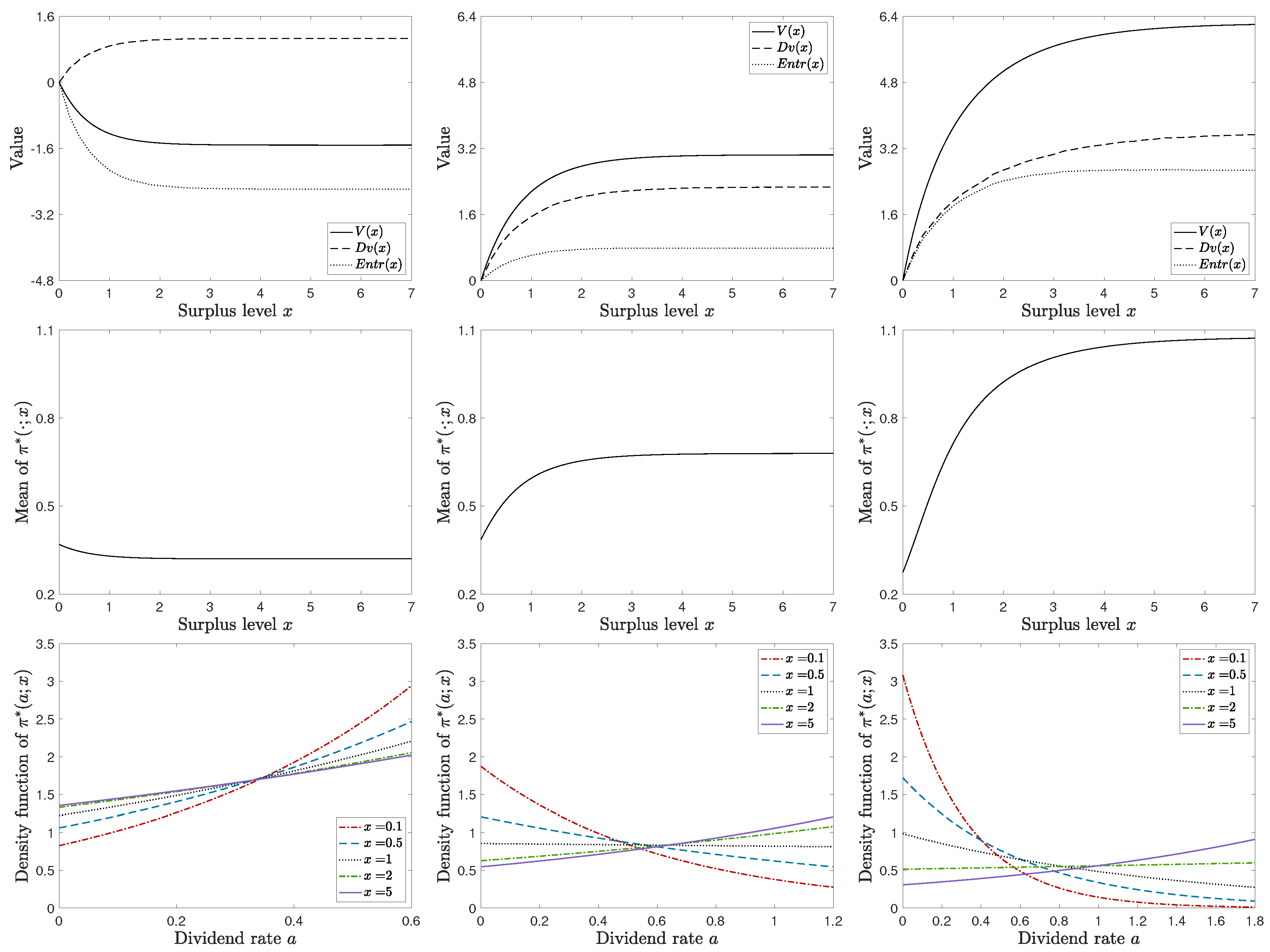
First, let $\lambda =1.5$, $M=0.6$. Then $M<d_1\left(\lambda \right)$ and it belongs to Case 1. Note that $V\left(x\right)$ in this case is decreasing and non-positive, as a sharp contrast to the results of classical dividend problem. The figure on the top row, left column of Figure 3 plots the corresponding value function and its two components $Dv\left(x\right)$ and $Entr\left(x\right)$.3 The figure on the middle row, left column of Figure 3 plots the mean of the optimal distribution ${\pi }^{*}(·;x)$, which is decreasing on x. The figure on the bottom row, left column of Figure 3 shows the density function of the optimal distribution with respect to different surplus level x. Because $V^{\prime }\left(x\right)\le 0$, the optimal distribution is a truncated exponential distribution with rate $-\lambda /\left(1-V^{\prime }\left(x\right)\right)<0$ for any $x\ge 0$. Therefore, it is more likely to pay high dividend rate. Furthermore, as surplus x increases, the density function becomes more flat because $V^{\prime }\left(x\right)$ is increasing to 0 and the rate $-\lambda /\left(1-V^{\prime }\left(x\right)\right)$ is decreasing on x.

Second, let $\lambda =1.5$, $M=1.2$. Then $d_1\left(\lambda \right)<M<d_2\left(\lambda \right)$ and it belongs to Case 2 (i). The figure on the top row, middle column of Figure 3 shows the corresponding value function, $Dv\left(x\right)$ and $Entr\left(x\right)$. In contrast to Case 1, $Entr\left(x\right)$ in this case becomes positive since M is sufficiently large, making the value function $V\left(x\right)$ positive. The figure on the middle row, middle column of Figure 3 plots the mean of the optimal distribution ${\pi }^{*}(·;x)$, which is increasing on x. The figure on the bottom row, middle column of Figure 3 shows the density function of optimal distribution with respect to different surplus level x. When x is small, it is more likely to choose a low dividend paying rate, because paying too high dividend rate would probably cause the insurance company to go bankruptcy and harms the shareholder’s benefit in the long run. When x becomes larger, it is more likely to pay high dividend rate.

Third, let $\lambda =1.5$, $M=1.8$. Then $M>d_2\left(\lambda \right)$ and it belongs to Case 2 (ii). The figure on the top row, right column of Figure 3 shows the corresponding value function, $Dv\left(x\right)$ and $Entr\left(x\right)$. In this case, the limit of $V\left(x\right)$ is higher than that of the classical value function $V_{cl}\left(x\right)$, which is $M/\rho =6$. Note that the expected total discounted dividends under exploratory policy $Dv\left(x\right)$ does not exceed that of the classical policy $V_{cl}\left(x\right)$, because the classical optimal dividend policy fully exploits the known environment. For sufficiently large M and $\lambda$, $Entr\left(x\right)$ is large enough to make $V\left(x\right)$ larger than $V_{cl}\left(x\right)$. The figure on the middle row, right column of Figure 3 plots the mean of the optimal distribution ${\pi }^{*}(·;x)$ and the figure on the bottom row, right column of Figure 3 plots the density function of the optimal distribution, which are similar to that of Case 2 (i).

When $\lambda =1.5$, $M=0.7662$, it belongs to Case 3 and the value function in this case should be constantly zero.

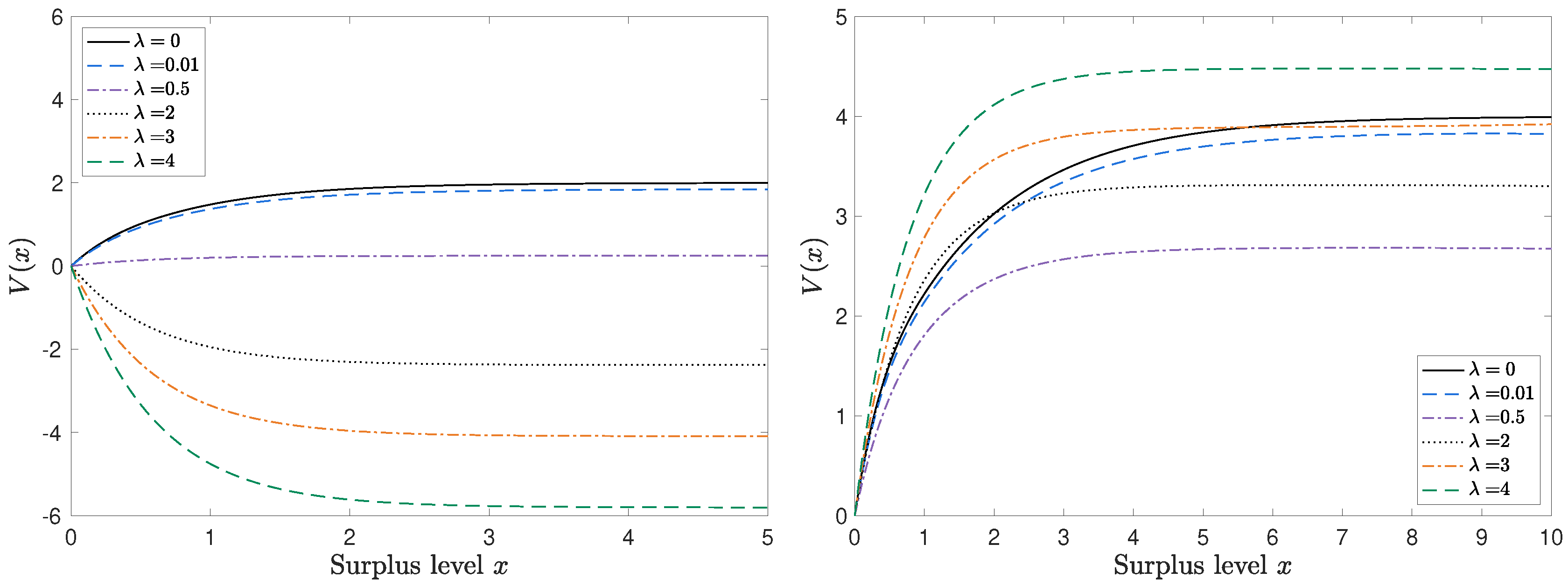
We also vary the value of $\lambda$ while keeping the other parameter values unchanged. Figure 4 shows the value function under different values of $\lambda$ with $M=0.6$ and $M=1.2$ respectively. Note that when $\lambda =0$, $V\left(x\right)$ degenerates to the classical value function $V_{cl}\left(x\right)$. For $M=0.6$, it is Case 2 (ii) when $\lambda$ is small and then becomes Case 3 and Case 1 as $\lambda$ getting larger. As aforementioned, it cannot be Case 2 (ii) since $M<1$. Indeed, the left panel of Figure 4 shows the value function could not exceed the classical one as $\lambda$ getting smaller. On the other hand, for $M=1.2$, it can only be Case 2 and even Case 2 (ii) if $\lambda$ is large enough. The right panel of Figure 4 shows the value function is always increasing on x for different values of $\lambda$ and it can exceed the classical value function for a sufficiently large $\lambda$.

6. Conclusion

This paper studies the dividend optimization problem in the entropy regularization framework. In an unknown environment, the entropy is incoprated into the objective function to encourage the exploration and an exploratory dividend policy is introduced. We establish the exploratory HJB equation, we find that the optimal distributional control is a truncated exponential distribution. Compared to the classical value function, the value function in the exploratory dividend problem is classified into three cases. The monotonicity of the value function is determined by the maximal dividend paying rate and the temperature parameter which controls the weight of exploration.

One future research direction is to consider the exploratory dividend policy under the non-exponential discounting which makes the problem time-inconsistent. Furthermore, reinsurance could also be considered as part of the insurance company’s strategy in addition to the dividend policy, which is more technically challenging under the entropy regularization framework. Finally, one could take other definitions of the entropy, instead of the Shannon’s differential, as a measure of the level of exploration in reinforcement learning.

References

1. Wang, H.; Zariphopoulou, T.; Zhou, X.Y. Reinforcement Learning in Continuous Time and Space: A Stochastic Control Approach. Journal of Machine Learning Research 2020, 21, 1–34. [Google Scholar]
2. Lundberg, F. Approximerad framställning af sannolikhetsfunktionen. Återförsäkring af kollektivrisker. Akademisk afhandling; Almqvist &Wiksells, 1903.
3. De Finetti, B. Su un’impostazione alternativa della teoria collettiva del rischio. Transactions of the XVth international congress of Actuaries. New York, 1957, Vol. 2, pp. 433–443.
4. Gerber, H.U. Entscheidungskriterien für den zusammengesetzten Poisson-Prozess. PhD thesis, ETH Zurich, 1969.
5. Schmidli, H. Stochastic control in insurance; Springer Science & Business Media, 2007.
6. Jeanblanc-Picqué, M.; Shiryaev, A.N. Optimization of the flow of dividends. Uspekhi Matematicheskikh Nauk 1995, 50, 25–46. [Google Scholar] [CrossRef]
7. Asmussen, S.; Taksar, M. Controlled diffusion models for optimal dividend pay-out. Insurance: Mathematics and Economics 1997, 20, 1–15. [Google Scholar] [CrossRef]
8. Jgaard, B.H.; Taksar, M. Controlling risk exposure and dividends payout schemes: insurance company example. Mathematical Finance 1999, 9, 153–182. [Google Scholar] [CrossRef]
9. Asmussen, S.; Højgaard, B.; Taksar, M. Optimal risk control and dividend distribution policies. Example of excess-of loss reinsurance for an insurance corporation. Finance and Stochastics 2000, 4, 299–324. [Google Scholar] [CrossRef]
10. Azcue, P.; Muler, N. Optimal reinsurance and dividend distribution policies in the Cramér-Lundberg model. Mathematical Finance: An International Journal of Mathematics, Statistics and Financial Economics 2005, 15, 261–308. [Google Scholar] [CrossRef]
11. Azcue, P.; Muler, N. Optimal investment policy and dividend payment strategy in an insurance company. The Annals of Applied Probability 2010, 20, 1253–1302. [Google Scholar] [CrossRef]
12. Gaier, J.; Grandits, P.; Schachermayer, W. Asymptotic ruin probabilities and optimal investment. The Annals of Applied Probability 2003, 13, 1054–1076. [Google Scholar] [CrossRef]
13. Kulenko, N.; Schmidli, H. Optimal dividend strategies in a Cramér–Lundberg model with capital injections. Insurance: Mathematics and Economics 2008, 43, 270–278. [Google Scholar] [CrossRef]
14. Yang, H.; Zhang, L. Optimal investment for insurer with jump-diffusion risk process. Insurance: Mathematics and Economics 2005, 37, 615–634. [Google Scholar] [CrossRef]
15. Choulli, T.; Taksar, M.; Zhou, X.Y. A diffusion model for optimal dividend distribution for a company with constraints on risk control. SIAM Journal on Control and Optimization 2003, 41, 1946–1979. [Google Scholar] [CrossRef]
16. Gerber, H.U.; Shiu, E.S. On optimal dividend strategies in the compound Poisson model. North American Actuarial Journal 2006, 10, 76–93. [Google Scholar] [CrossRef]
17. Avram, F.; Palmowski, Z.; Pistorius, M.R. On the optimal dividend problem for a spectrally negative Lévy process. The Annals of Applied Probability 2007, 17, 156–180. [Google Scholar] [CrossRef]
18. Yin, C.; Wen, Y. Optimal dividend problem with a terminal value for spectrally positive Levy processes. Insurance: Mathematics and Economics 2013, 53, 769–773. [Google Scholar] [CrossRef]
19. Zhao, Y.; Kosorok, M.R.; Zeng, D. Reinforcement learning design for cancer clinical trials. Statistics in medicine 2009, 28, 3294–3315. [Google Scholar] [CrossRef] [PubMed]
20. Komorowski, M.; Celi, L.A.; Badawi, O.; Gordon, A.C.; Faisal, A.A. The artificial intelligence clinician learns optimal treatment strategies for sepsis in intensive care. Nature medicine 2018, 24, 1716–1720. [Google Scholar] [CrossRef]
21. Mirowski, P.; Pascanu, R.; Viola, F.; Soyer, H.; Ballard, A.J.; Banino, A.; Denil, M.; Goroshin, R.; Sifre, L.; Kavukcuoglu, K. ; others. Learning to navigate in complex environments. arXiv:1611.03673. [CrossRef]
22. Zhu, Y.; Mottaghi, R.; Kolve, E.; Lim, J.J.; Gupta, A.; Fei-Fei, L.; Farhadi, A. Target-driven visual navigation in indoor scenes using deep reinforcement learning. 2017 IEEE international conference on robotics and automation (ICRA). IEEE, 2017, pp. 3357–3364. [CrossRef]
23. Radford, A.; Jozefowicz, R.; Sutskever, I. Learning to generate reviews and discovering sentiment. arXiv:1704.01444. [CrossRef]
24. Paulus, R.; Xiong, C.; Socher, R. A deep reinforced model for abstractive summarization. arXiv:1705.04304. [CrossRef]
25. Mnih, V.; Kavukcuoglu, K.; Silver, D.; Rusu, A.A.; Veness, J.; Bellemare, M.G.; Graves, A.; Riedmiller, M.; Fidjeland, A.K.; Ostrovski, G.; others. Human-level control through deep reinforcement learning. Nature 2015, 518, 529–533. [Google Scholar] [CrossRef] [PubMed]
26. Jaderberg, M.; Czarnecki, W.M.; Dunning, I.; Marris, L.; Lever, G.; Castaneda, A.G.; Beattie, C.; Rabinowitz, N.C.; Morcos, A.S.; Ruderman, A.; others. Human-level performance in 3D multiplayer games with population-based reinforcement learning. Science 2019, 364, 859–865. [Google Scholar] [CrossRef] [PubMed]
27. Silver, D.; Huang, A.; Maddison, C.J.; Guez, A.; Sifre, L.; Van Den Driessche, G.; Schrittwieser, J.; Antonoglou, I.; Panneershelvam, V.; Lanctot, M.; others. Mastering the game of Go with deep neural networks and tree search. Nature 2016, 529, 484–489. [Google Scholar] [CrossRef]
28. Silver, D.; Schrittwieser, J.; Simonyan, K.; Antonoglou, I.; Huang, A.; Guez, A.; Hubert, T.; Baker, L.; Lai, M.; Bolton, A.; others. Mastering the game of go without human knowledge. Nature 2017, 550, 354–359. [Google Scholar] [CrossRef]
29. Auer, P.; Cesa-Bianchi, N.; Fischer, P. Finite-time analysis of the multiarmed bandit problem. Machine learning 2002, 47, 235–256. [Google Scholar] [CrossRef]
30. Cesa-Bianchi, N.; Gentile, C.; Lugosi, G.; Neu, G. Boltzmann exploration done right. Advances in neural information processing systems 2017, 30. [Google Scholar]
31. Todorov, E. Linearly-solvable Markov decision problems. Advances in neural information processing systems 2006, 19. [Google Scholar]
32. Ziebart, B.D.; Maas, A.L.; Bagnell, J.A.; Dey, A.K. ; others. Maximum entropy inverse reinforcement learning. Aaai. Chicago, IL, USA, 2008, Vol. 8, pp. 1433–1438.
33. Nachum, O.; Norouzi, M.; Xu, K.; Schuurmans, D. Bridging the gap between value and policy based reinforcement learning. Advances in neural information processing systems 2017, 30. [Google Scholar]
34. Wang, H.; Zhou, X.Y. Continuous-time mean–variance portfolio selection: A reinforcement learning framework. Mathematical Finance 2020, 30, 1273–1308. [Google Scholar] [CrossRef]
35. Dai, M.; Dong, Y.; Jia, Y. Learning equilibrium mean-variance strategy. Mathematical Finance 2023, 33, 1166–1212. [Google Scholar] [CrossRef]
36. Bai, L.; Gamage, T.; Ma, J.; Xie, P. Reinforcement Learning for optimal dividend problem under diffusion model. arXiv:math/2309.10242. [CrossRef]
37. Tang, W.; Zhang, Y.P.; Zhou, X.Y. Exploratory HJB equations and their convergence. SIAM Journal on Control and Optimization 2022, 60, 3191–3216. [Google Scholar] [CrossRef]
38. Gao, X.; Xu, Z.Q.; Zhou, X.Y. State-dependent temperature control for Langevin diffusions. SIAM Journal on Control and Optimization 2022, 60, 1250–1268. [Google Scholar] [CrossRef]
39. Strulovici, B.; Szydlowski, M. On the smoothness of value functions and the existence of optimal strategies in diffusion models. Journal of Economic Theory 2015, 159, 1016–1055. [Google Scholar] [CrossRef]
1
For example, the dividend paying rate under the threshold strategy is the maximal rate if the surplus exceeds the threshold; otherwise, it pays nothing. Since the threshold is determined by the model parameters, the change in the estimated parameters may dramatically change the dividend paying rate from zero to the maximal rate, or conversely.
2
We apply the shooting method which adjusts the initial value of first-order derivative such that the boundary conditions (14) and (20) are satisfied and use “ode45” function in Matlab to find the numerical solution to (19).
3
For each initial surplus x, we discretize the continuous time into small pieces ( Δ t = 0.0005 ) and sample 2000 independent surplus processes X t π * to simulate D v ( x ) and E n t r ( x ) .
Figure 1. The classical value functions (top) and the optimal dividend-paying rate (bottom) for μ = 1 , σ = 1 , ρ = 0.3 , M = 0.6 (left panels), M = 1.2 (middle panels), and M = 1.8 (right panels), respectively.
Preprints 91638 g001
Figure 2. Cases of value functions given M and λ .
Preprints 91638 g002
Figure 3. Let μ = 1 , σ = 1 , ρ = 0.3 , λ = 1.5 . Let M = 0.6 (left column); M = 1.2 (middle column); M = 1.8 (right column), respectively. The figures on the top row show the value function V ( x ) , the expected total discounted dividends D v ( x ) and the expected total weighted discounted entropy E n t r ( x ) . The figures on the middle row show the mean of the optimal distribution π * ( · ; x ) . The figures on the bottom row show the density function of the optimal distribution with respect to different surplus level x.
Preprints 91638 g003
Figure 4. The value function V ( x ) given different values of λ with M = 0.6 (left) and M = 1.2 (right)
Preprints 91638 g004
Disclaimer/Publisher’s Note: The statements, opinions and data contained in all publications are solely those of the individual author(s) and contributor(s) and not of MDPI and/or the editor(s). MDPI and/or the editor(s) disclaim responsibility for any injury to people or property resulting from any ideas, methods, instructions or products referred to in the content.
Copyright: This open access article is published under a Creative Commons CC BY 4.0 license, which permit the free download, distribution, and reuse, provided that the author and preprint are cited in any reuse.
Prerpints.org logo
Preprints.org is a free preprint server supported by MDPI in Basel, Switzerland.
Subscribe
© 2024 MDPI (Basel, Switzerland) unless otherwise stated