
Submitted:
28 November 2023
Posted:
29 November 2023
You are already at the latest version
Abstract
This paper presents an approach to enhancing the clarity and intelligibility of speech in digital communications compromised by various background noises. Utilizing deep learning techniques, specifically a Variational Autoencoder (VAE) with 2D convolutional filters, we aim to suppress background noise in audio signals. Our method focuses on four simulated environmental noise scenarios: storms, wind, traffic, and aircraft. Training dataset has been obtained from public sources (TED-LIUM 3 dataset, which includes audio recordings from the popular TED-TALK series) combining with these background noises. The audio signals were transformed into 2D power spectrograms, upon which our VAE model was trained to filter out the noise and reconstruct clean audio. Our results demonstrate that the model outperforms existing state-of-the-art solutions in noise sup-pression. Although differences in noise types were observed, it was challenging to definitively conclude which background noise most adversely affects speech quality. Results have been assessed with objective methods (mathematical metrics) and subjective (listening to a set of audios by humans). Notably, wind noise showed the smallest deviation between the noisy and cleaned audio, perceived subjectively as the most improved scenario. Future work involves refining the phase calculation of the cleaned audio and creating a more balanced dataset to minimize differences in audio quality across scenarios. Additionally, practical ap-plications of the model in real-time streaming audio are envisaged. This research contributes significantly to the field of audio signal processing by offering a deep learning solution tailored to various noise conditions, enhancing digital communication quality.
Keywords:
Speech enhancement
; Noise suppression
; Deep learning
; Variational autoencoders
1. Introduction
Signal processing is the storage, edition or transmission of a signal, either in analog or digital form [1]. Sound, after the acquisition and transformation of acoustic waves into electrical ones, becomes a signal that can be processed. [2] shows the first approached the particular method of treating audio as an electrical signal. Digital processing was introduced later by converting a sound signal into a piece of information of binary numbers using an Analogue-to-Digital Converter (ADC). On the other hand, the Digital-to Analogue Converter (DAC) is used to transform a digital signal into an analog one.
The quality of the digital signal depends on two features: sampling rate and bit depth. The first one indicates the number of samples per second obtained from the original audio [3]. If we want excellent audio quality, we need a high sample rate to capture a more accurate signal so that the digital version could be more similar to the original one. The second feature indicates the number of bits of storage for each audio sample [4]. These factors are directly related to the different storage formats. For example, one minute of a high-quality recording in WAV format requires 10 Megabytes of storage.
Although the quality used to store audio allows them to be very faithful to the originals, some information may be lost during transmission. In particular, we call noise to that signal or set of signals that distort the wave that transmits the original sound. Within this concept there can be artificial noises (those generated by the means of communication, such as interferences) or natural noises (those generated by the environment where the communication takes place). When the transmission is in noisy scenarios, ambient sounds may affect the intelligibility of the received message.
The motivation for this research arises from the critical need to enhance the clarity and intelligibility of speech in various communication settings, where background noise often compromises the quality of transmitted audio. While existing noise reduction techniques have made strides in mitigating this issue, our work aims to develop a deep learning model specifically tailored to suppress background noise across a range of simulated scenarios. However, our objectives extend beyond mere noise elimination. We also seek to quantitatively assess the relative difficulty of filtering out different types of background noises present in the same audio fragment. By doing so, we aim to identify which types of noise have a more detrimental impact on speech quality, thereby a guide for future research and technological development in the field of audio signal processing.
The real problem comes when the noise is equal to or stronger than the signal and causes its complete distortion. This fact opens up the possibility of using techniques that can eliminate background noise for safer and more reliable transmissions, which is desirable in cases such as phone communications, especially in emergency situations.
Artificial intelligence has demonstrated its ability to remove noisy information from various formats, such as images or signals [5,6]. Deep learning models have obtained the best results in recent years among all the artificial intelligence techniques. Deep learning was defined by Lecun [7] as models composed of multiple processing layers that learn representations of data with various levels of abstraction. These models have shown exemplary performance in speech enhancement [8].
Audio signals can be analyzed either in the time domain or the frequency domain, with the latter often represented visually as images. Our approach capitalizes on the image-processing capabilities of convolutional layers in deep learning neural networks, specifically for tasks like cleaning and restoration. We have trained a deep learning model that can remove four types of background noise with pairs of original audio and audio mixed with background noise. Original audio signals have been transformed into a 2D representation by converting it into a power spectrogram. Following this transformation, we employ a two-dimensional Variational Autoencoder (VAE) to remove noise from the signal and reconstruct the clean audio. As no particular dataset solves the presented use cases, we have created our own. To carry out the model development and training we have used a dataset with recordings of TED talks (TED-LIUM 3 dataset) as expected output and the same dataset mixed with four different background noises (aircrafts, rain and thunderstorms, wind and traffic) obtained from different specialized websites as input to the network.
Results show that our model performs better than other solutions in the state of the art. Regarding the proposed scenarios, although there are differences between them, we cannot assure that one of the background noises influence more than others. The only, thing confirmed by the results is that the audios with wind are perceived with better improvement, but this perception is a bit tricky as the differences between the clean audios and the audios with this background noise are smaller.
The paper is structured as follows. Section 2 compiles some works framed in speech enhancements, audio denoising, etc. Section 3 formally describes the dataset used to train the model and the deep learning models used in the research. Section 4 compiles the different results that have been obtained and their interpretation. Finally, section 5 gives some conclusions and future works.
2. State of the Art
Building on the foundational need to improve speech communication in noisy environments, as outlined in our introduction, a variety of models have been developed to address challenges in speech enhancement and background noise reduction. This section aims to review these related works, highlighting their contributions and limitations, to contextualize our own approach, which extends beyond mere noise removal to a nuanced understanding of how different types of noise uniquely impact speech quality.
Some of these works apply techniques not encompassed in the deep learning field. [9] reduces the presence of background music over conversational audios. It uses trigonometric transformation and wavelet denoising techniques. In [10], the audio denoising is made with speech audios and noises like buzzing equipment or background noise from the street. Spectrograms form the training dataset and use a block thresholding estimation procedure. The same authors present in [11] a similar approach to suppressing the harmonic noise of music by using its spectrograms. The method applies block attenuation techniques. Finally, [12] implement a process to denoise speech audios containing slight background noises (which do not work with loud ones). It works with raw audio and applies Wiener filters, a well-known method of the previous age of audio denoising.
The present work focuses on speech enhancement but uses deep learning techniques. The following studies make use of these methods in similar use cases. In [13], an autoencoder with a bottleneck that uses Recurrent Neural Networks (RNNs) addresses speech enhancement in recordings made with mobile phones. In [14], the audios are isolated from videos. The work uses two models combining convolutional networks and Fourier transformations. One model detects that a person is speaking, and another isolate the speech. The use of Generative Adversarial Networks (GANs) for speech enhancement can be found in [15]. In this case, they used raw audios of 10 use cases (8 of them are genuine cases and 2 of them artificially created). Another interesting work is [16], which separates the different waves of raw audios with voices of women and men mixed with songs. In this case, deep autoencoders are used to achieve the issue. To end,
Another distinguishing feature is the use of power log spectrograms to train the deep learning model, as in [17] that eliminates background noise from factories in conversational audios of Japanese people. The approach uses a deep autoencoder and spectrograms. In [18], RNNs detect if a person is speaking and predict the voice without background noise. The dataset consists of spectrograms with white noise, traffic jams, and street environments. In [19], a Long Short-Term memory neural network (LSTM) is trained with frequency spectrograms to improve the speech quality in audios with background noises, reverberations, and a poor communication environment. Another work that uses power spectrograms is [20], which represents cases of passing cars and café babble noise. It uses a convolutional neural network in the approach. Similar, there is [21] that use voice sound with background noises characteristics of conversations represented as spectrograms. Then, a deep neural network of 4 layers is used to eliminate the noise in the spectrograms. Finally, [22] use a type of Autoencoder called U-Net with spectrograms that account for the wave's phase in the audio.
This research stands out in the field due to several key innovations. Primarily, it targets evaluating the impact of four distinct real-world background noises on speech audios. To achieve this, we have developed a unique deep learning model designed to effectively eliminate these noises from a series of speech recordings. Our choice of a variational autoencoder for this purpose distinguishes our approach. Moreover, our study is the first of its kind to incorporate a subjective evaluation method. This involves a panel assessing the clarity of speech audios post noise-removal. While other studies rely solely on mathematical metrics, our approach adds a crucial human dimension to the assessment. This step is often overlooked in other research due to the technical challenges and potential information loss when converting spectrograms back into raw audio, possibly leading to subpar results that others might choose not to report. Our willingness to undertake this complex transformation and evaluation process further underlines the novelty and depth of our work.
3. Materials and Methods
In this paper we have trained a deep learning model, specifically a Variational Autoencoder, with pairs of power logs spectrograms of voice audios mixed with four different background noises: aircrafts, rain and thunderstorms, wind and traffic jams. The research followed a four-step process that are described following. First, the creation of the dataset by mixing speech audios with background noise. Second, the transformation of the audios into a visual representation, a spectrogram, that is more efficient to manage by the model. Third, the training of the model with the dataset. Finally, the objective and subjective evaluations. The workflow followed from working with the raw data until obtaining the trained model is represented in Figure 1.
3.1. Datasets of Speech Audios and Background Noises
3.1.1. Audio Features Decision
The first step consists of selecting the audio files format and the signal processing characteristics: sampling rate, bit-depth, and the number of channels. As file format, we use WAV or WAVE (apocope of Waveform), launched in 1991 by Microsoft based on RIFFF (Resource Interchange File Format) specification. It has the advantage of being an uncompressed format, in which the user hears what is stored. It also supports different quality characteristics such as sampling frequency and bit depth [23], which are the most important features for audio management [24]. We have decided to use 22.5 kHz, a bit-depth of 16 bits and only one audio channel corresponding to monaural sound re-production. These characteristics are sufficient and adequate for the problem we want to solve.
During the second step, we need to create the pairs of audios. As no particular dataset solves the presented use cases, we have created our own. For that, we need speech audios and background noises that represent the four use cases.
For the former, we are using the TED-LIUM 3 dataset, which includes audio recordings of the well-known TED-TALK series. The dataset contains 2,351 audio files in NIST Sphere format (SPH), which is very common in audio speech files as it includes the audio alongside a transcription of the speech. It uses a sampling rate of 16 kHz and a bit-depth of 16 bits. The total length of the dataset reaches more than 452 hours. In the audios, we can find a diverse range of people with different types of tones and quality recordings under other circumstances, which augments the problem's difficulty. The dataset is freely available to download from Open Speech and Language resources.
For the latter, we have obtained the different background noises from two websites. They used WAV format, a sampling rate of 16 kHz, and a bit-depth of 16. The number of audios per use case differs, as the availability was not the same. This problem will be, lately, solved during the preprocessing stage. Also, the length of the audio varies depending on the use case. Table 1 summarizes this information for the four use cases.
3.1.2. Audio Preprocessing
The first problem arose with the TED LIUM dataset as it has an SPH format. We transformed it into WAV format using a Python script using the SoX tool [25] to convert the audio.
Next, we describe all the modifications done to obtain the final dataset of pairs of audios. First, we have eliminated the first and last 15 seconds of the speech audios to avoid moments without speech and irrelevant sounds like applause or music. Then, we generated 60,000 chunks with a length of 3 seconds with a balance of 25% in-stances for each use case. At this stage, we have also set the value of the sampling rate, bit-depth, and the number of channels, which have been set at 22.5 kHz, 16 bits, and audio-mono channel, respectively. In the case of finding audio with different value ranges, the corresponding transformation applies min-max normalization. This method allows all audio values to be in the same range between 0.0 and 1.0. as shown in Equation 1.
Given the complexity of the problem, the neural model requires many audios for proper training. In our case, the availability of audios is scarce, so it has been necessary to apply data augmentation techniques and create synthetic data. Once we have the audios chunked in pieces of 3 seconds with standardized features, we have mixed the speech audios with the different background noises randomly but ensure the number of audios for the four use cases. In the cases where the background noise does not have a length of 3 seconds, different audio of the same case is chosen until the speech audio length is reached.
3.1.3. Visual Representation of Audios
Audio signals can be processed as a time-domain or a frequency domain representation. The former uses the signal as raw audio. The latter uses images of visual representations of the audio. Due to the high complexity of the problem where the original speech audios and its version with background noise do not match any of the values (increasing the difficulty of a reconstruction problem), we have decided to use the second option as images perform well in auto-encoders. We use autoencoders with convolutional filters of 2 dimensions which have demonstrated better performances in these models than those of 1 dimension [26].
Many audio representations in the frequency domain are log power spectrograms (LPS), Mel spectrograms, or Mel-frequency cepstral coefficients spectrograms (MFCCS). In this case, we are using LPS because it includes an audio feature called power representing wave decibels at a particular moment. LPS consists of an image representing the audio information. In this case, it captures more information than other standard spectrums, [27].
Spectrograms are created using a Python script and a library called librosa, [28], which specializes in music and audio management. The script implements a Short-Term Fourier Transformation (STFT) that converts the audio from the time domain to the frequency domain. Each spectrogram was created using a sliding window of 23 widths and 11.6 steps in milliseconds. The output spectrograms had a size of 256x256x1 for each instance. Finally, the dataset contains 60,000 spectrograms belonging to 15,000 for each use case.
3.2. Using a Variational Autoencoder for Noise Suppression
As noted in the state-of-the-art section, autoencoders perform well to do speech enhancement, audio denoising, etc. We have selected a variational autoencoder as the DL model to perform this task because of its ability to represent the input data more accurately using a latent space. With this representation, the output images have higher definition, and therefore the quality when transforming them backwards into raw audio will be better. In the following, we formalize some deep learning concepts to better understand this type of architecture.
3.2.1. Convolutional Operator
This operator lets to find image features like edges, which is why their main application is image classification [29]. In particular, it led to the creation of the 2-Dimensional Convolutional Neural Networks (2D CNNs) used in Deep Learning since 1999 [30]. Convolutional operators al-low finding a feature in one part of an image that can later be found in another. As we work with images of power log spectrograms, the convolutional operators of the Variational Autoencoder will find feature representations from one spectrogram to another.
3.2.2. Autoencoders
These two-part models first use a multilayer encoder network to represent high-dimensional structures in a low-dimensional space. Then, there is a decoder network to convert the data from this space into high-dimensional structures with some relations to the first one [31]. This architecture works as follows. The input data go through the different convolutional layers of the encoder, obtaining a small piece of data with the main features. These data are dis-tributed in the bottleneck, creating a representation called latent space. Finally, the feature representation goes through the decoder to obtain an output like the input data.
3.2.3. Variational Autoencoders
This Autoencoder solves the problem that classical ones have with the latent space. Instead of placing a single point in the latent space, this case provides a distribution. This latent space can also be better organized by adding a regularization to the loss function, [32]. In our case, it creates a distribution using the input data's mean and variance. The following Equation represents the distribution of this space.
Where represents the mean vector of the different distributions in the latent space, and |∑| the covariance matrix of the distributions. The last two parameters are calculated using Equations 3, and 4 applied to a space of 2 dimensions.
To sample a point into the latent space, we have used the formula of sampling points, depicted in Equation 5. In this case, we have modified it to get negative values, so we have a more expansive dimensional space to represent the information where ε is a sampled point from a standard normal distribution.
3.3. Training Phase
To train the model, we have split the dataset into a percentage of 80 for training/validation and 20 for the test. The final dataset has an amount of 60,000 LPS that represent audios of 3 seconds without overlapping. The model was trained with pairs of audios with mixed background noise and the original version of these audios.
The hyperparameters during training were found using a grid search strategy. This method guides the training in finding the best hyperparameter setting for the model by using different combinations of the values [33]. The different hyperparameters and values used in the grid search have been compiled in the Table 2.
Optimizer and loss function hyperparameters have not been changed during the process. Optimizer is an adaptive learning rate optimization algorithm. In particular, we have used Adam as it was explicitly designed for training deep neural networks, [34]. All the efforts to create a variational bottleneck do not make sense unless the network knows how to learn about the input data representations in the latent space. Therefore, the loss function needs a change to distribute the information in the latent space precisely and accurately. The loss function uses the Root Mean Squared Error (RMSE) and the Kullback-Leibler divergence DKL(P||Q) (KL). This last metric will allow the network to check if the distributions are placed correctly in the latent space. RMSE and KL have been formalized in Equations 6 and 7.
where N(μ,σ) is a normal distribution having as mean the mean µ and as standard deviation the standard deviation σ of the output data obtained in training and N(0,1) is the standard normal distribution.
Finally, Equation 8 shows the modified loss function we have used.
In this case, α is a hyperparameter that weights the KL metric. After fine tuning, the selected value for this hyperparameter was 100,000, indicating that the RMSE be-tween the input and output signals was not a primary concern in our optimization process. This decision was based on the understanding that RMSE is relatively poor metric for evaluating the noise level in an audio signal, especially when the audio is represented as an image in the form of a power spectrogram. In such a representation, even a minor deviation in a single pixel can significantly impact the RMSE, but this does not necessarily translate to a perceptible error when the image is converted back to an audio signal. Therefore, our model's loss function is designed to prioritize other aspects over RMSE for a more accurate and meaningful evaluation of audio quality.
The model comprises 306,762,465 hyperparameters, and we used an AMD Threadripper 2950X with 128 Gigabytes of DDR4 RAM and a GeForce RTX 2080 TI GPU. The training lasted more than 22 hours. The final metric at the end of the training phase was 0.0153.
3.4. Proposed Method
The proposed solution is a two-dimensional VAE that is trained with pairs of spectrograms of speech audios with real background noise and the original speech audios. After some convolutional operation, the encoder reduces the size to a minimal piece of information that represents its main features. These pieces of information are then placed in a latent space, which is a distribution of the encoded data obtained at the convolutional stage. The mean and variance of each input is used to fit the distribution in the latent space, this feature being the main difference from a standard encoder. For a VAE, each input represents a distribution in latent space rather than a single point. Information is recovered and upsampled from the latent space until the output has the expected dimensions. Finally, this output is compared to the spectral representation of the original audio without background. This comparison evaluates how well the background noise has been suppressed and lets the model adjust its hyperparameters and learn the information. After training with the whole dataset that comprises audios from the four use cases, the model can remove real background noise.
The input layer of the model has a size of 256x256x1, representing the audio of one channel, which is connected to the following layer. The input layer aims to feed the audio to the convolutional blocks. These blocks are responsible for reducing the dimensionality of the information. The convolutional stage consists of 6 convolutional blocks, where each of them obtains a feature map of the previous data. Each block has two convolutional layers with two 2-dimensional filters of size 3x3, stride one, and max-pooling of 2x2 (except in the last block). Convolutional layers in the same block have the same number of neurons using Rectified Liner Unit (ReLU) as an activation function. The number of neurons from one block to another is the following: 32, 64, 128, 256, 512, and 1,024. At the end of this convolutional stage, the input data has been reduced to 8x8x1,024. This small piece of information represents the input data with all the main features. Finally, a flattened layer is applied to process information as a one-dimensional vector of size 65,536.
At this point, the information goes through the bottleneck, which in the case of VAEs builds a latent space of its representation. The bottleneck entrance has a dense layer of 2,048 neurons that introduces the information from the last convolutional block. Then, we have two other dense layers that manage the distribution's mean and variance, having 2,048 neurons. A lambda layer is applied to choose the point representing the input data in the latent space. After getting this point, we can position it in a multivariate space and recreate the last convolution dimensions before the bottleneck, allowing the decoder to do the inverse process. To start this process, we use a dense layer that converts the point into information that can be processed in the de-convolutional stage.
The stage of dimensionality upsampling, or deconvolution, now begins. This stage starts with a reshape layer so the information can be introduced in the two dimensions' deconvolutional blocks of 2 dimensions. This process has five deconvolution blocks. Each block comprises two convolution layers, with an upsampling layer in the first position. Again, the number of neurons within the layers of the same block is the same, and all use the ReLU activation function. The number of neurons per layer of each block is 512, 256, 128, 64, and 32. These blocks increase the dimensionality of the feature map. In this deconvolution process, starting from the tiny feature map in the bottleneck stage, new audio spectrograms are created using only the essence of the original audio. In each convolution block, concatenate layers have been used with the even blocks of the encoder to speed up the training and not lose the substantial relationship between the data. Lastly, a final convolution layer with one neuron is used to achieve the same final audio size as the input. The last layer uses the hyperbolic tangent (tanh) activation. A representation of the model is in Figure 2.
Finally, the output data is compared to the spectral representation of the original audio without background noise. This comparison evaluates how well the back-ground noise has been suppressed and lets the model adjust its hyperparameters and learn the information. After feeding the whole dataset that comprises audios from the four use cases, the model is trained so it can remove real background noise.
4. Results and Evaluation
This section compiles the results obtained by evaluating the model for the four different use cases with objective and subjective tests. The first ones compare our model with others in the state of the art using mathematical metrics. The second type of tests are based on the subjective perception of a group of people who will evaluate how good the model is at eliminating noise.
4.1. Objective Evaluations
4.1.1. Evaluation of Noise Reduction Performance
We will assess the performance of our approach in eliminating background noise by comparing it with two baseline methods. This evaluation involves comparing the noisy audio input to the model with the model's output, which is a denoised signal. The two baseline models are a classical method using Wiener filters and a more recent technique known as Deep Audio Priors Design (DAP). Wiener filters were used by [35] to reduce the noise in audios utilizing the frequency domain. DAP Design is an update of U-Net that uses dilated convolutions and dense connections [36].
The evaluation has been made with a set of audios that comprises 400 instances, 100 for each use case. Each audio has a length of 3 seconds, with a sample rate of 22 kHz and a bid-depth of 16.
To make an accurate comparison, we use two metrics: MSE and Signal to Noise Ratio (NSR). The first one measures the Euclidean distance between two images that are the spectrograms of an audio with background noise and the same audio after being processed by the denoising model, [37]. The larger the value of MSE, the greater the difference between the noise signal and the cleaned signal, from which it can be inferred that the model eliminates background noise better. The metric is depicted in the Equation 9 where is the value of a particular position in the noisy audio, and a value of the denoising audio in the same place.
The second metric measures the difference in decibels (dB) between the same two signals once they have been converted back to the audio domain. SNR values range between -35 and 35 dB, which is the theoretical magnitude of noise. The closer the value is to zero (either positive or negative), the better the performance of the model [38]. Equation 10 mathematically formalized this metric.
In Table 3, we compile both metrics and compare our model with the two pro-posed baselines.
It is important to note that MSE is not an accurate metric for assessing audio quality. When starting with an image that is essentially a Fourier transform of an audio signal, converting it back to an audio signal using the inverse transform doesn't necessarily reflect how well the audio will turn out. Even a minor change in a single pixel can drastically alter the sound obtained upon reversing the transformation. This fact is due to the use of a parameter of the original audio called the phase of the wave. This parameter is lost when transforming the audio into spectrogram and a change in its value can made the audio obtained after transforming back the spectrogram into something inaudible. In our case, we have used the Inverse STF, and we have used the phase of the audio with noise that is used as an input in the model. Although the results are not perfect, the evaluation demonstrate that are good enough but should be improved in the future.
Therefore, MSE values do not precisely represent differences in the quality of the resulting sound. However, we can assert that if the MSE is very low, the two images are highly similar at the pixel level. This implies that the spectrogram obtained after the noise-cleaning process is highly like the original (noisy) one that was fed into the model meaning that the cleaning process worked poorly. Therefore, while MSE may not be a perfect indicator of audio quality, it does serve as a useful metric for evaluating how closely the processed image resembles the original one in terms of pixel-level similarity. SNR works with the converted signal and reflects whether the amount of noise in the signal is high or low. Combination of both metrics provides a more comprehensive evaluation of the model's performance in both the image and audio domains.
Based on the results shown in Table 3, our model outperforms in all scenarios, reducing both the image noise and the actual noise in the subsequently converted signal. In terms of MSE, Wiener filters perform poorly across all four use cases, as the audios being compared are nearly identical. DAP Design shows better results, but it's important to note that this method removes all information, including the speech, resulting in silent audio. Obviously, in this case, the MSE value should be high, as noisy audio differs significantly from silent audio. MSE can still be calculated when comparing images, even if the audio signal itself is inaudible. Regarding the Signal-to-Noise Ratio (SNR), our model significantly outperforms Wiener filters. On the other hand, DAP Design's approach leads to silent audio, rendering the SNR value empty.
When we look at the results for different situations, it seems that storm and rain noises are easier to eliminate when evaluated using both MSE and SNR metrics. When considering the standard deviation, instances involving wind noise tend to yield poorer results in some examples. This variability in performance across different types of environmental noise underscores the complexity of the problem and the need for a more nuanced approach to noise reduction in audio signals.
4.1.2. Evaluation of Background Noise Suppression Based on Noise Type
This evaluation quantifies the differences between the spectrogram of the original audio, sourced from the TED-LIUM 3 dataset before adding background noise, and two other spectrograms: one corresponding to the audio with background noise and the other to the denoised audio. The relationship between these values serves as a measure of the level of noise suppression relative to the original clean signal. In other words, it helps us identify which type of background noise has been most effectively suppressed. By referencing both values to the same baseline—the original TED talk audio that is free of noise—we obtain a common metric for all scenarios. The difference between these metrics indicates the effectiveness of noise reduction in each case. Specifically, the better the second measurement (difference between the restored audio spectrogram and the original audio spectrogram) is compared to the first (difference between the noisy audio spectrogram and the original audio spectrogram), the more effectively the background noise has been eliminated in that particular use case.
We will use two metrics applied to the spectrograms: again, the MSE and the Structural Similarity Index Measure (SSIM). SSIM was introduced by Wang et al. (2004) and measures the perceptual similarity between images regardless of which is of better quality. It considers three image features: luminance (l), contrast (c), and structure (s) that are weighted through three constants: α, β, and γ. SSIM is calculated using Equation 11:
This evaluation has used the 100 samples for each scenario from the previous evaluation. So, 400 instances have been evaluated in total.
For both metrics, the same analysis can be applied. The suppression of wind noise yields the poorest performance. Both in absolute terms and as a percentage, the difference in MSE and SSIM values is the smallest. In the case of MSE, which measures pixel-to-pixel similarity between spectrograms, the restored audio does resemble the original more than the noisy audio does, but by a smaller percentage (37.2%) com-pared to other scenarios. It's worth noting that these are the cases that most closely resemble the original audio, meaning that the distortion introduced by the noise is the lowest among all use cases. Therefore, the margin for improvement is smaller as will be reflected in the subjective assessment where noise cleanliness depends on auditory perception. In the other scenarios, although the MSE of the restored audio is still high, the reduction compared to the audio with background noise is much greater. Specifically, in the case of thunderstorms and rainfall, the quality of the work is significantly higher. This is also noteworthy considering that these types of background noise most severely affect the intelligibility of the original spoken segments. A similar analysis and conclusions apply when considering the SSIM metric instead of MSE. In this case, storms are the best, wind is the worst and traffic interchange its position with aircrafts. The results of Table 4 confirm what the comparison with the baselines describes in Table 3.
4.2. Subjective Tests
We present an evaluation based on listening to audios. In this case, we have created a set of audios that comprises the four use cases that have been listened to by a group of people to evaluate the amount of background noise that has been suppressed. The dataset consists of 22 different audios; for each audio, the volunteers must listen to the audio with background noise and the same audio after being processed by our model. For each of the four use cases, there were four different audios, totaling 20 audios. The two remaining audios correspond to control audios where no background noise was eliminated and have been used to check that the surveyed people were performing the test well.
During the process, volunteers could listen to each pair of audios as often as possible. Then, they must choose between four different options: "No or practically no noise eliminated", "Some noise eliminated", "Much noise eliminated" and "All or almost all noise eliminated". The evaluation was delivered through a Google Form, and 61 people answered it. All the information has been compiled in Figure 3. The top pie chart represents the average results of the evaluation of the 20 valid audios. The other pie charts depict the evaluation results for each of the use cases.
Looking at the figure above, we can conclude that most of the people think that the model could suppressed much noise or almost all (90%). Only in a few cases (10%), the evaluation result on no noise eliminated. If we look at the use cases separated, there are no big differences obtaining evaluations where good evaluations (from much noise to all noise) are around percentages of 90%. It should be highlighted that wind scenario is the one with more cases of removing all the noise which corroborates the objective evaluations obtained with the mathematical metrics (the margin for improvement is less than in the other cases). If we looked at the scenarios considering that at much noise is eliminated storms/wind is the one that performs the best, but differences are not remarkable. Another interesting point is that wind/storms, rain and traffic are the scenarios that have reported cases where no noise was eliminated.
5. Conclusions and Future Work
Audio signals can be processed either in the time domain, treating the raw signal, or in the frequency domain. In the latter case, visual representations of the audio (images) are used. This research proposes a model for cleaning background noise in audio signals (human speech) using a VAE composed of 2D convolutional filters applied to a two-dimensional representation of the audio signal, namely power log spectrograms. In the research, we propose four different scenarios that simulate environmental noise produced by storms, wind, traffic jams and aircrafts. The whole workflow of the research comprises different stages. First, we created an ad-hoc dataset by mixing speech audios with background noises representing the four use cases. Then, we have used this dataset to train a VAE with pairs of audios with background noise and only the speech audio using spectrograms. To measure if we have trained the model accurately, we have used objective and subjective measures. Objective measures allow to measure mathematically which is the scenario where the background noise is more difficult to suppress and if the proposed model overcomes other models proposed before. The subjective evaluation allows to confirm the previous results based on the auditive perception of some people. Subjective evaluations are normally not per-formed in the works compiled in the state of the art as there is a need to transform the spectrograms into audios so they can be listened by the surveyed people. This transformation is not easy to apply as it depends on the phase that corresponds to the original speech clean audio. In our case, we have applied the IFTF that although it does not achieve perfect results, it does obtain perfectly evaluable audios by using the phase of the audios that are input for the model.
Mathematical metrics produced by our model confirm that it performs better than the selected baselines in all cases. If we look at the results between use cases, we can see that storms and rains are easier to eliminate. Looking at the standard deviation, we can see that wind cases have worse results in a few examples. In this case, it should be highlighted that the scenario of background wind is the one with the smallest differences between the noisy audio and the cleaned one. This is confirmed in the objective evaluation where surveyed people evaluate this scenario as the one with best performance.
As future works, the main need is to obtain a method that could calculate in a more precise way the phase of the cleaned audio. Also, there is a need to obtain a more balanced dataset where the differences between the audio with background noise and the audio after using the model are smaller between scenarios. From practical perspective, the model could be integrated into applications, so the model works with streaming audio.
6. Patents
The Spanish Patent and Trademark Office (OEPM) has processed the patent application related to the work presented in this article, assigning it the number P202330047 and the filing date of January 24, 2023.
Author Contributions
Conceptualization, AN and AJGT; methodology, AN; software, JCC; validation, AN, JCC and AJGT; formal analysis, AN, JCC and AJGT; investigation, AN and AJGT; resources, AJGT; data curation, JCC; writing—original draft preparation, AN; writing—review and editing, AN and AJGT; supervision, AJGT and AN; project administration, AJGT; funding acquisition, AJGT. All authors have read and agreed to the published version of the manuscript.
Funding
This research received no external funding.
Data Availability Statement
Publicly available datasets were analyzed in this study. TED-LIUM dataset data can be found here: https://www.openslr.org/51/. Background noises can be obtained from https://www.videvo.net/es/efectos-de-sonido/viento/ and https://zenodo.org/record/4279220#.YpdZVKhByUk
Conflicts of Interest
The authors declare no conflict of interest.
References
- Thon, L.E. (2003). 50 years of signal processing at ISSCC. 2003 IEEE International Solid-State Circuits Conference, 2003. Digest of Technical Papers. ISSCC., San Francisco, CA, USA, 2003, pp. 27-28. [CrossRef]
- Franks, L.; Witt, F. Solid-state sampled-data bandpass filters. 1960 IEEE International Solid-State Circuits Conference. Digest of Technical Papers. [CrossRef]
- Pras, A.; Guastavino, C. (2010). Sampling Rate Discrimination: 44.1 kHz vs. 88.2 kHz. In Audio Engineering Society Convention 128. Audio Engineering Society.
- Kipnis, A.; Goldsmith, A.J.; Eldar, Y.C. (2015). Optimal trade-off between sampling rate and quantization precision in Sigma-Delta A/D conversion. International Conference on Sampling Theory and Applications (SampTA), 2015, pp. 627-631. [CrossRef]
- Liu, B.; Liu, J. (2019, March). Overview of image denoising based on deep learning. In Journal of Physics: Conference Series (Vol. 1176, No. 2, p. 022010). IOP Publishing.
- Zie, J.; Colonna, J.G.; Zhang, J. Bioacoustic signal denoising: a review. Artificial Intelligence Review 2021, 54, 3575–3597. [Google Scholar] [CrossRef]
- LeCun, Y.; Bengio, Y.; Hinton, G. Deep learning. Nature 2015, 521, 436–444. [Google Scholar] [CrossRef]
- Yuliani, A.R.; Amri, M.F.; Suryawati, E.; Ramdan, A.; Pardede, H.F. Speech Enhancement Using Deep Learning Methods: A Review. Jurnal Elektronika dan Telekomunikasi 2021, 21, 19–26. [Google Scholar] [CrossRef]
- Hammam, H.; Elazm, A.A.; Elhalawany, M.E.; El-Samie, A.; Fathi, E. Blind separation of audio signals using trigonometric transforms and wavelet denoising. International Journal of Speech Technology 2010, 13, 1–12. [Google Scholar] [CrossRef]
- Yu, G.; Mallat, S.; Bacry, E. Audio denoising by time-frequency block thresholding. IEEE Transactions on Signal processing 2008, 56, 1830–1839. [Google Scholar] [CrossRef]
- Yu, G.; Bacry, E.; Mallat, S. (2007, April). Audio signal denoising with complex wavelets and adaptive block attenuation. In 2007 IEEE International Conference on Acoustics, Speech and Signal Processing-ICASSP'07 (Vol. 3, pp. III-869). IEEE.
- Ng, L.C.; Burnett, G.C.; Holzrichter, J.F.; Gable, T.J. (2000, June). Denoising of human speech using combined acoustic and EM sensor signal processing. In 2000 IEEE International Conference on Acoustics, Speech, and Signal Processing. Proceedings (Cat. No. 00CH37100) (Vol. 1, pp. 229-232). IEEE.
- Tan, K.; Zhang, X.; Wang, D. Deep learning based real-time speech enhancement for dual-microphone mobile phones. IEEE/ACM Transactions on Audio, Speech, and Language Processing 2021, 29, 1853–1863. [Google Scholar] [CrossRef] [PubMed]
- Afouras, T.; Chung, J.S.; Zisserman, A. The conversation: Deep audio-visual speech enhancement. arXiv 2018, arXiv:1804.04121. [Google Scholar]
- Pascual, S.; Bonafonte, A.; Serra, J. SEGAN: Speech enhancement generative adversarial network. arXiv 2017, arXiv:1703.09452. [Google Scholar]
- Abouzid, H.; Chakkor, O.; Reyes, O.G.; Ventura, S. Signal speech reconstruction and noise removal using convolutional denoising audioencoders with neural deep learning. Analog Integrated Circuits and Signal Processing 2019, 100, 501–512. [Google Scholar] [CrossRef]
- Lu, X.; Tsao, Y.; Matsuda, S.; Hori, C. (2013, August). Speech enhancement based on deep denoising autoencoder. In Interspeech (Vol. 2013, pp. 436-440).
- Valin, J.M. (2018, August). A hybrid DSP/deep learning approach to real-time full-band speech enhancement. In 2018 IEEE 20th international workshop on multimedia signal processing (MMSP) (pp. 1-5). IEEE.
- Pandey, A.; Wang, D. On cross-corpus generalization of deep learning-based speech enhancement. IEEE/ACM transactions on audio, speech, and language processing 2020, 28, 2489–2499. [Google Scholar] [CrossRef]
- Roy, S.K.; Nicolson, A.; Paliwal, K.K. (2020, October). A Deep Learning-Based Kalman Filter for Speech Enhancement. In INTERSPEECH (pp. 2692-2696).
- Nossier, S.A.; Wall, J.; Moniri, M.; Glackin, C.; Cannings, N. An experimental analysis of deep learning architectures for supervised speech enhancement. Electronics 2020, 10, 17. [Google Scholar] [CrossRef]
- Choi, H.S.; Kim, J.H.; Huh, J.; Kim, A.; Ha, J.W.; Lee, K. Phase-aware speech enhancement with deep complex u-net. arXiv 2019, arXiv:1903.03107. [Google Scholar]
- Siegert, I.; Lotz, A.F.; Duong, L.L.; Wendemuth, A. Measuring the impact of audio compression on the spectral quality of speech data. Studientexte zur Sprachkommunikation: Elektronische Sprachsignalverarbeitung 2016, 2016, 229–236. [Google Scholar]
- Kanetada, N.; Yamamoto, R.; Mizumachi, M. Evaluation of Sound Quality of High Resolution Audio. The Japanese Journal of the Institute of Industrial Applications Engineers 2013, 1, 52–57. [Google Scholar] [CrossRef]
- Sourceforge SoX-Sound. Available online: http://sox.sourceforge.net/ (accessed on 26 November 2023).
- Wu, N.; Wang, X.; Lin, B.; Zhang, K. A CNN-based end-to-end learning framework toward intelligent communication systems. IEEE Access 2019, 7, 110197–110204. [Google Scholar] [CrossRef]
- Repp, A.; Szapudi, I. Precision prediction of the log power spectrum. Monthly Notices of the Royal Astronomical Society: Letters 2017, 464, L21–L25. [Google Scholar] [CrossRef]
- McFee, B.; Raffel, C.; Liang, D.; Ellis, D.P.; McVicar, M.; Battenberg, E.; Nieto, O. (2015, July). librosa: Audio and music signal analysis in python. In Proceedings of the 14th python in science conference (Vol. 8, pp. 18-25).
- LeCun, Y.; Boser, B.; Denker, J.; Henderson, D.; Howard, R.; Hubbard, W.; Jackel, L. (1989). Handwritten digit recognition with a back-propagation network. Advances in neural information processing systems, 2.
- LeCun, Y.; Haffner, P.; Bottou, L.; Bengio, Y. (1999). Object Recognition with Gradient-Based Learning. In: Shape, Contour and Grouping in Computer Vision. Lecture Notes in Computer Science, vol 1681. Springer, Berlin, Heidelberg. [CrossRef]
- Hinton, G.E.; Salakhutdinov, R.R. Reducing the dimensionality of data with neural networks. Science 2006, 313, 504–507. [Google Scholar] [CrossRef] [PubMed]
- Kingma, D.P.; Welling, M. Auto-encoding variational bayes. arXiv 2013, arXiv:1312.6114. [Google Scholar]
- Bergstra, J.S.; Bardenet, R.; Bengio, Y.; K´egl, B. (2011). Algorithms for hyper-parameter optimization. In Advances in neural information processing systems (pp. 2546–2554).
- Kingma, D.P.; Ba, J. Adam: A method for stochastic optimization. arXiv 2014, arXiv:1412.6980. [Google Scholar]
- Lim, J.S.; Oppenheim, A.V. Enhancement and bandwidth compression of noisy speech. Proceedings of the IEEE 1979, 67, 1586–1604. [Google Scholar] [CrossRef]
- Narayanaswamy, V.S.; Thiagarajan, J.J.; Spanias, A. On the Design of Deep Priors for Unsupervised Audio Restoration. arXiv 2021, arXiv:2104.07161. [Google Scholar]
- Sammut, C.; Webb, G.I. (Eds.) (2011). Encyclopedia of machine learning. Springer Science & Business Media.
- Elkum, N.; Shoukri, M.M. Signal-to-noise ratio (SNR) as a measure of reproducibility: design, estimation, and application. Health Services and Outcomes Research Methodology 2008, 8, 119–133. [Google Scholar] [CrossRef]
Figure 1.
Workflow for training a model for background noise suppression.
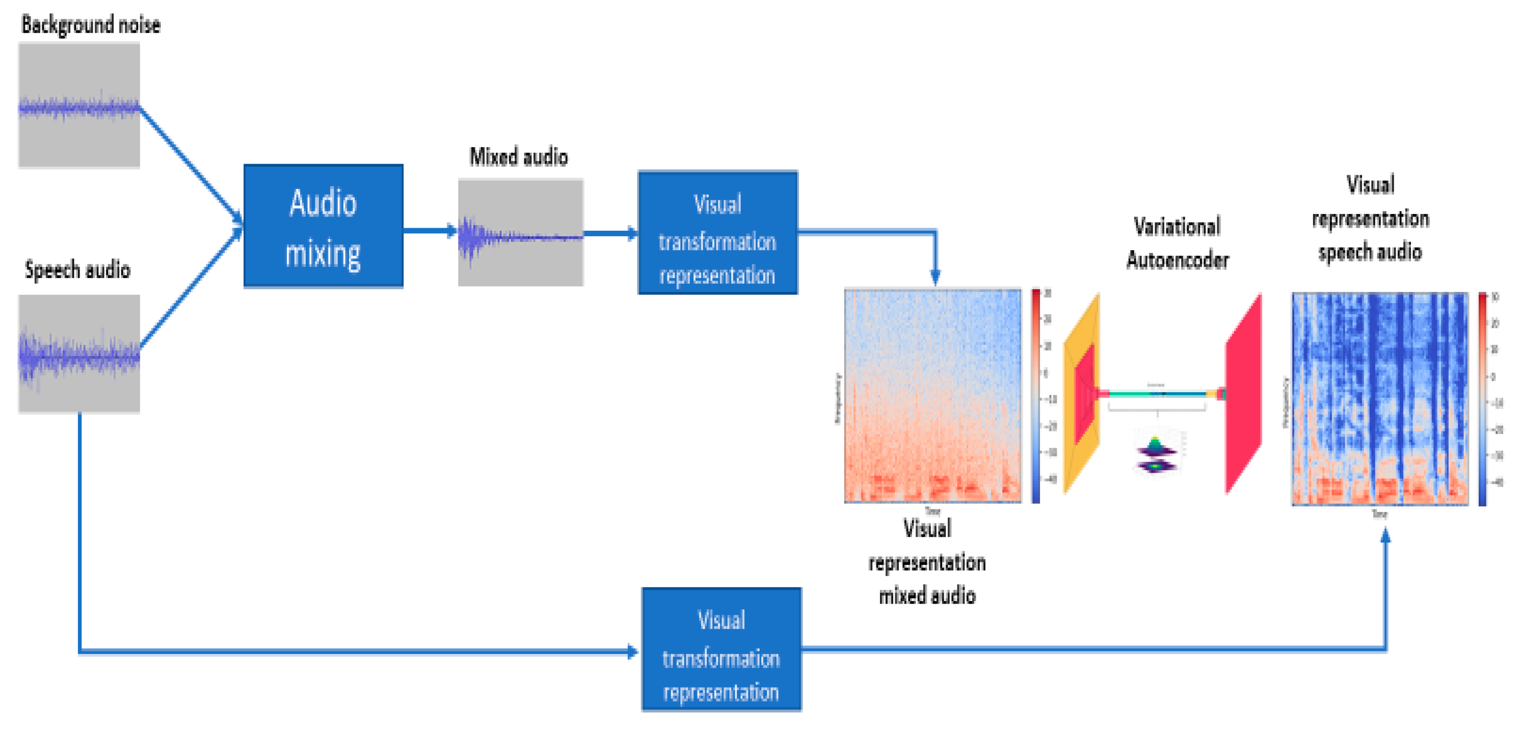
Figure 2.
Architecture of the model.
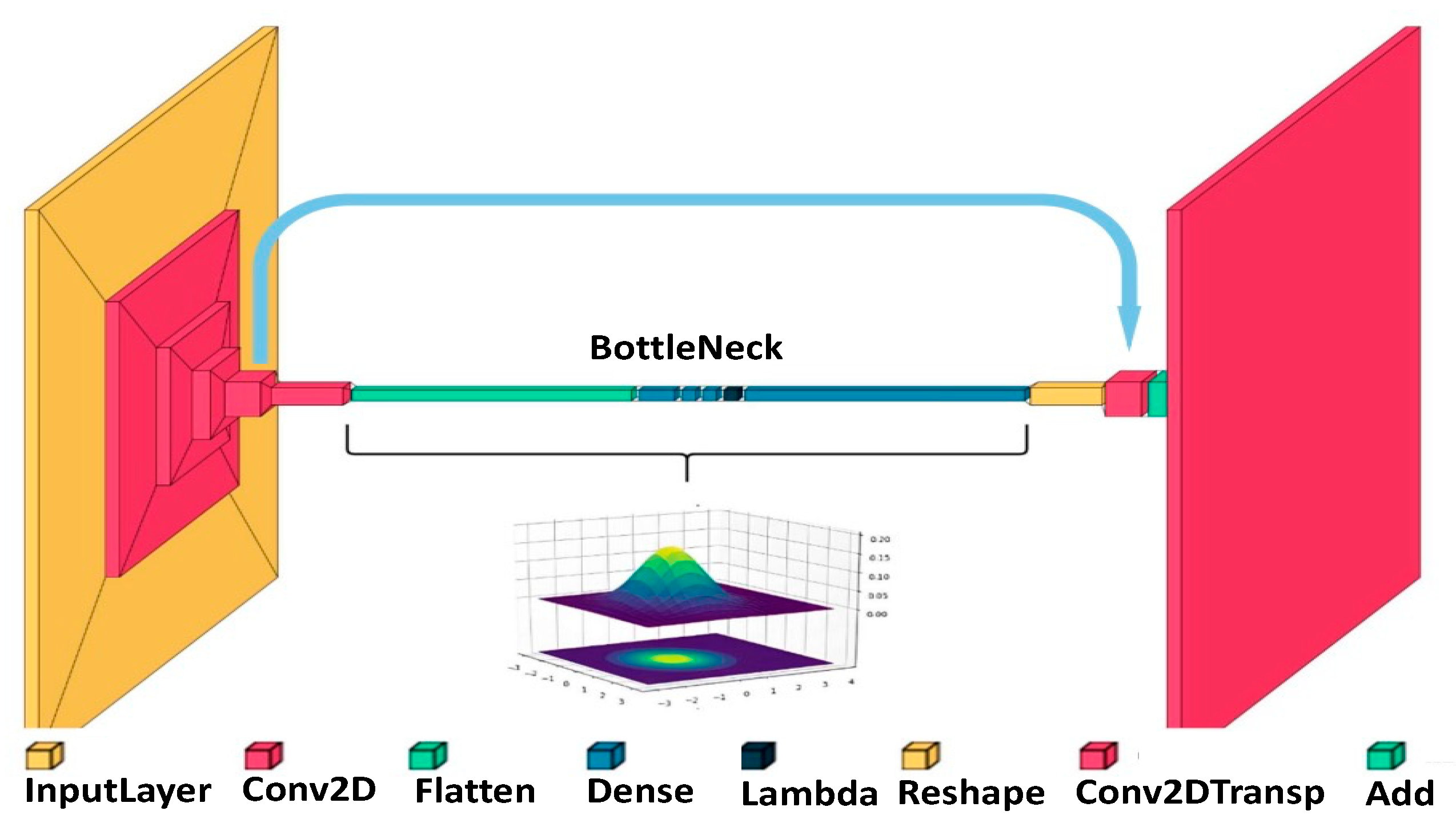
Figure 3.
Human evaluation of noise suppression by listening to a set of audios.
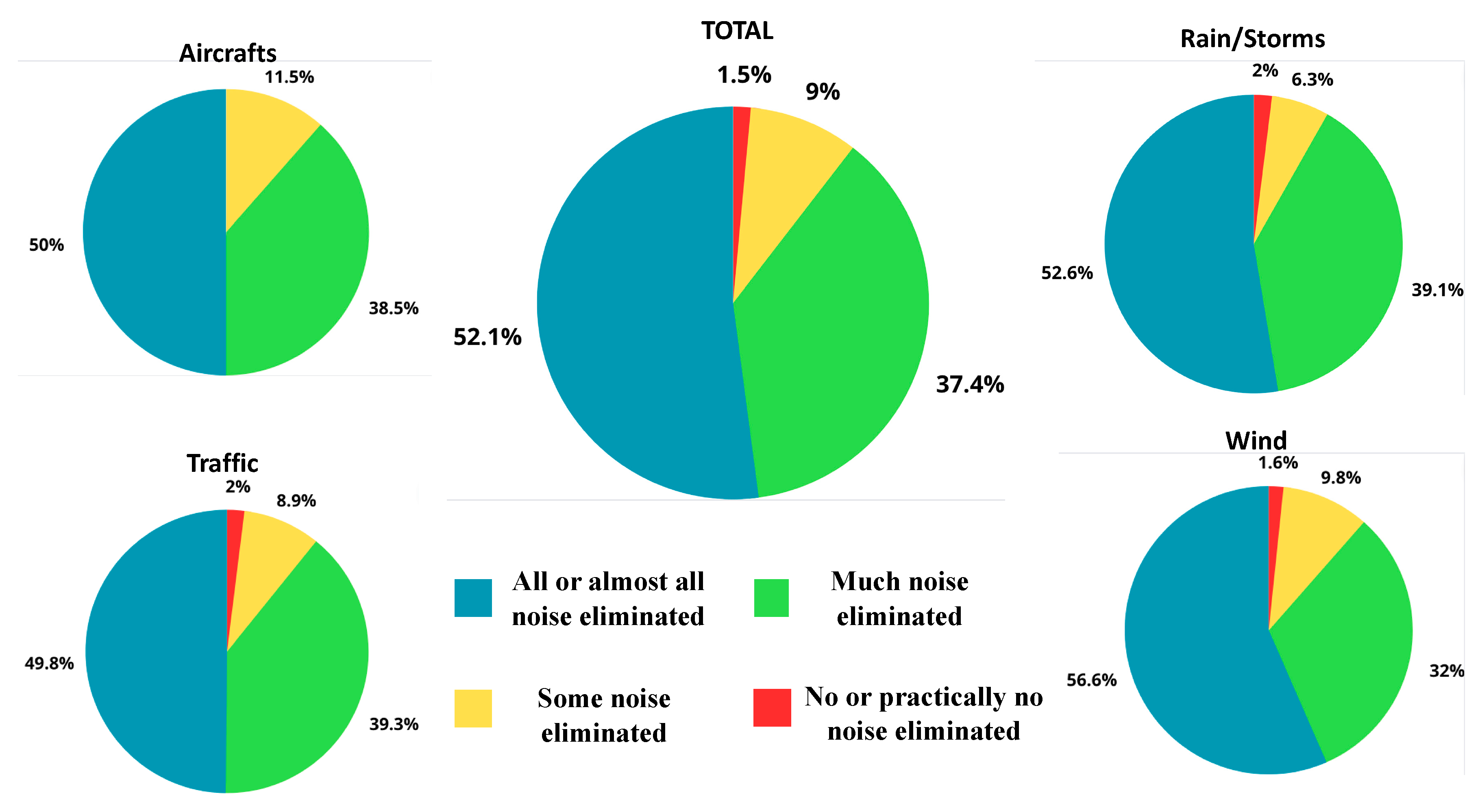

Table 1.
Background noise use cases dataset.
| Use case | Number of audios | Length per audio |
|---|---|---|
| Aircrafts | 80 | Around 5 seconds |
| Storm lights and rain | 18 | Around 5 minutes |
| Wind | 522 | From 3 seconds to 5 minutes |
| Traffic jams | 512 | Around 3 seconds |
Table 2.
Hyperparameters and values used in the grid search.
| Hyperparameter | Values |
|---|---|
| Latent space | 128, 200, 400, 800, 1,024 and 2,048 neurons |
| Dense layer | 100, 200, 256, 1,024, 2,48 and 4,096 neurons |
| Convolutional blocks | 3, 4, 5 and 6 |
| Skip connections | 3, 4 and 5 |
| Learning rate | 0.01, 0.001 and 0.0001 |
Table 3.
Comparison against baselines.
| Use case | MSE | SNR | |
|---|---|---|---|
| Aircrafts | Wiener | 0.0006 ± 0.0035 | 16.378 ± 7.4762 |
| DAP Design | 0.0761 ± 0.1621 | - | |
| Our model | 0.0182 ± 0.0234 | 1.3702 ± 0.8983 | |
| Storms and rain | Wiener | 0.0007 ± 0.0064 | 16.908 ± 6.8374 |
| DAP Design | 0.0877 ± 0.0879 | - | |
| Our model | 0.0202 ± 0.0758 | -1.2728 ± 3.7621 | |
| Traffic jams | Wiener | 0.0006 ± 0.0036 | 17.328 ± 13.1234 |
| DAP Design | 0.0693 ± 0.3245 | - | |
| Our model | 0.0154 ± 0.2522 | 0.4991 ± 1.3253 | |
| Wind | Wiener | 0.0004 ± 0.0003 | 17.505 ± 9.6523 |
| DAP Design | 0.0687 ± 0.0319 | - | |
| Our model | 0.0182 ± 0.9325 | -0.1870 ± 3.2167 | |
Table 4.
Comparison between spectrograms.
| Use case | MSE | SSIM | |
|---|---|---|---|
| Aircrafts | Noisy audio | 1,628 ± 1,246 | 0.6173 ± 0.1257 |
| Restored audio | 680 ± 323 | 0.6257 ± 0.1012 | |
|
Absolute difference % reduction |
948 58,2% |
-0.0084 -1,4% |
|
| Storms and rain |
Noisy audio | 1,867 ± 1,100 | 0.5780 ± 0.0848 |
| Restored audio | 698 ± 267 | 0.6075 ± 0.0754 | |
|
Absolute difference % reduction |
1,169 62,6% |
-0.0375 -5,1% |
|
| Traffic jams | Noisy Audio | 1,329 ± 1,139 | 0.6282 ± 0.1127 |
| Restored audio | 609 ± 349 | 0.6437 ± 0.0891 | |
|
Absolute difference % reduction |
720 54,2% |
-0.0155 -2,5% |
|
| Wind | Noisy audio | 683 ± 541 | 0.7287 ± 0.1107 |
| Restored audio | 429 ± 174 | 0.7311 ±0.0769 | |
|
Absolute difference % reduction |
209 37,2% |
-0.0024 -0,3% |
Disclaimer/Publisher’s Note: The statements, opinions and data contained in all publications are solely those of the individual author(s) and contributor(s) and not of MDPI and/or the editor(s). MDPI and/or the editor(s) disclaim responsibility for any injury to people or property resulting from any ideas, methods, instructions or products referred to in the content. |
© 2023 by the authors. Licensee MDPI, Basel, Switzerland. This article is an open access article distributed under the terms and conditions of the Creative Commons Attribution (CC BY) license (http://creativecommons.org/licenses/by/4.0/).
Copyright: This open access article is published under a Creative Commons CC BY 4.0 license, which permit the free download, distribution, and reuse, provided that the author and preprint are cited in any reuse.


