
Submitted:
29 November 2023
Posted:
29 November 2023
You are already at the latest version
Abstract
This article combines the traditional definition of portfolio risk with minimum spanning tree based “interconnectedness risk" to improve the equal risk contribution portfolio performance. We use betweenness centrality to measure an asset’s importance in a market graph (network). After filtering the complete correlation network to a minimum spanning tree, we calculate the centrality score and convert it to a centrality heuristic. We develop an adjusted variance-covariance matrix using the centrality heuristic, to bias the model to assign peripheral assets in the minimum spanning tree higher weights. We test this methodology using the constituents of the S&P 100 index. The results show that the centrality equal risk portfolio can improve upon the base equal risk portfolio returns, with a similar level of risk. We observe that during bear markets, the centrality-based portfolio can surpass the base equal risk portfolio risk.
Keywords:
networks
; portfolio optimization
; equal risk portfolio
; asset allocation
; centrality
; market graph
1. Introduction
Traditionally in finance, risk is described by the variance of asset returns. In this article we extend the consideration of risk to include the risk (“interconnectedness” risk) based on minimum spanning tree topology. The goal of this article is to show that by taking this broader risk consideration into account we can improve the equal risk contribution (ERC) portfolio performance. We use the constituents of the S&P100 index to illustrate the improvement in the portfolio’s risk- adjusted return.
Modern portfolio theory (MPT) measures the risk of an asset by its volatility/variance (Markowitz 1952). Higher volatility assets carry higher risk. With the introduction of MPT, (Markowitz 1952) also introduced the mean variance portfolio (MVO). MVO portfolios rely on predicted asset returns and a variance-covariance (VCV) matrix to create a portfolio that minimizes risk while aiming for a specific expected return.
Generally, the expected returns and VCV matrix are estimated based on historical returns. As shown in (Chopra and Ziemba 1993), the risk and return estimations can carry large errors, making the MVO portfolio unstable. Since the bulk of the estimation error lies in the return estimation, one way to improve the portfolio is by only using the VCV matrix to optimize asset allocations (Chopra and Ziemba 1993). Such strategies are called risk-based strategies. The simplest example of this is the minimum variance (MV) portfolio (the risk-only alteration of the MVO portfolio). While MV portfolios are more stable than MVO portfolios, they lack diversification. This is due to the optimization model concentrating funds in the assets with the lowest volatility. In contrast, the ERC portfolio allocates the weights so each asset contributes equal risk to the total portfolio risk (Maillard et al. 2010). This means each asset will have a non-zero weight, thus creating a diversified portfolio from the pool of assets. The ERC portfolio is often compared with the equal weighted (EW) portfolio (Maillard et al. 2010).
In comparison to MPT, market graphs are a fairly recent way to analyze the market. The introduction of market graphs (networks) by (Mantegna 1999) allowed for another way to understand asset relationships. Market graphs are a hierarchical organization of the assets in consideration (Mantegna 1999). Analysis of these networks can provide information about asset relationships and how risk is transferred between assets (Konstantinov et al. 2020). Market graphs are typically developed based on correlations between assets.
In each network, the assets (typically stocks) are the nodes, and edges connecting the nodes are dictated by the correlations between the assets (Mantegna 1999). The graph can be filtered into a minimum spanning tree (MST), which retains only the most important relationships in the full network ((Mantegna 1999); (Tumminello et al. 2005)). Within the study of networks, centrality is a key network property that helps us understand how important a node is within a network (Rodrigues 2019). Centrality can be quantified in various ways, of which five common methods are; betweenness centrality, closeness centrality, eigenvector centrality, eccentricity and degree centrality (Pozzi et al. 2013). Recently there has been more research on the use of centrality and MSTs to improve portfolio performance. Such articles on centrality based portfolios show that portfolio performance can be improved by favouring the peripheral assets in a graph (Peralta and Zareei 2016,Pozzi et al. 2013). In (Pozzi et al. 2013), the authors explain that peripheral asset portfolios preform better since central assets are more likely to carry more risk in comparison to peripheral assets, as they are subject to more sudden changes. As well, as shown in (Baitinger and Papenbrock 2017), the risk associated with a stock’s importance in the network (“interconnectedness” risk) is not related to the risk captured by the VCV matrix.
So far, network-based risk using MSTs has been used to improve MVO and MV portfolio construction. Most of this literature does not consider other important portfolio models such as those based on ERC. The contribution of this paper is to demonstrate that by considering both “interconnectness” risk and VCV risk concepts, we can improve on the ERC portfolio risk-return performance. We do this by simply augmenting the VCV matrix with the MST topology information.
The rest of the paper is organized as follows; Section 2 reviews the current literature in the area of network based portfolios. Section 3 presents the methodology of centrality-based portfolio construction. Section 4 gives the experimental framework and computational results for centrality-based ERC portfolios. We present the conclusions of this work in Section 5.
2. Literature Review
Since the introduction of market graphs (Mantegna 1999), many articles have studied the various aspects of financial networks and their applications (Boginski et al. 2005,Bonanno et al. 2001,Onnela et al. 2003,Tumminello et al. 2005). (Onnela et al. 2003) is one of the first articles to study changes in network topology (primarily MSTs) over time. The authors concluded two key findings. Firstly, during a crisis, the stocks become highly correlated causing the tree to shrink. Secondly, the authors found that the stocks in a minimum variance portfolio tend to be on the peripheral of the tree. Following this study, networks have also been used to study systemic risk within financial networks (Huang et al. 2009,Huang et al. 2016,Lai and Hu 2021).
Using networks to build a portfolio is not a new concept. Networks have previously been used to develop portfolios via the use of clustering. As done in (Tola et al. 2008), (Puerto et al. 2020) and (Boginski et al. 2014), clustering can be used to select assets for a portfolio to improve its performance. However, recently there has been more interest in the concept of using the asset relationships understood from networks to improve the portfolio weights and attain better portfolio performance (better risk-adjusted return).
(Pozzi et al. 2013) studied the portfolios consisting of only central assets of a network and compared them to portfolios only consisting of peripheral assets. The results showed that peripheral asset portfolios preformed better than the central asset portfolios. (Li et al. 2019) also presented similar results using the centrality heuristic introduced by (Pozzi et al. 2013) in combination with using market mode to filter noise and improve basic MVO and EW portfolio performance. The idea of asset returns being negatively linked to asset centrality was also confirmed by (Peralta and Zareei 2016). Based on the findings of articles like (Pozzi et al. 2013), (Onnela et al. 2003) and (Peralta and Zareei 2016), there have been many articles showcasing the various ways MSTs and centrality can be used to improve traditional portfolio methods. (Baitinger and Papenbrock 2017) calculated the optimal asset allocations by using the the five centrality measures discussed in (Pozzi et al. 2013). Using the base MVO model, the authors minimized (peripheral assets weighted more) or maximized (central assets weighted more) each centrality measure instead of the more traditional risk measure, portfolio variance. The results highlighted that centrality based (centrality minimizing) portfolios can out-preform traditional portfolios methods. (Baitinger and Papenbrock 2017) also found that the “interconnectedness risk" (risk based on network relationships) were not related to the risk captured by the VCV matrix. Therefore combining the two can help improve traditional portfolio methods.
Table 1 provides a summary of some current relevant literature on the use of centrality measures to improve traditional portfolio methods. Many of the articles in Table 1 focus on the improvement of the MVO or MV portfolios. The key distinguishing factor between each of the articles is how they have implemented the centrality information (typically based on MST) into the traditional optimization methods. Some articles use constraints (Výrost et al. 2019), while others use a multi-objective approach (Giudici et al. 2022). Some authors, such as (Peralta and Zareei 2016), implemented the centrality within the closed form solution (which allows short-selling). Instead of only using centrality for the purposes of asset allocation, (Cho and Song 2023), (Zhao et al. 2018) and (Peralta and Zareei 2016) use centrality measures to select the assets for a portfolio. Centrality is not the only way to measure a node’s importance in a network. (Clemente et al. 2021) uses the local clustering coefficient (similar to measuring local density in a network (Hansen et al. 2011)) to improve the MV portfolio. To calculate the local clustering coefficient, the authors use threshold filtering, which discards the edges with weight less than a given threshold. The authors implement the local clustering coefficient by using a modified matrix instead of the VCV matrix when calculating the optimal weights. The modified matrix uses the local clustering coefficient to represent the asset relationships, instead of the covariance, and scales the coefficients using the variances of the assets. Naïve equal risk portfolios are also commonly combined with network centrality. The key difference is naïve ERC portfolios do not take into account the asset covariance, while traditional ERC portfolios do. One such article is (Kaya 2013), which uses eccentricity to scale the weights of the naïve equal risk portfolio. (Konstantinov et al. 2020) demonstrates how eigenvector centrality, based on factor-asset networks, can be used to outpreform the MV, naïve ERC and EW portfolios.
(Lopez de Prado 2016) presented a novel technique called hierarchical risk parity (HRP). HRP is an ERC based strategy using network information to improve portfolio performance. However the HRP portfolio method uses the hierarchical nature of a network via hierarchical clustering and not by directly studying network measures like centrality. Other articles, such as (Ricca and Scozzari 2024), use networks to develop mixed integer formulations for portfolio optimization, which include the network topology information in the objective function (multi-objective problem) or as constraints.
In contrast, we find little literature concerning the improvement of more complex portfolios like ERC with centrality and MST. (Clemente et al. 2022) is one of the few articles in which the authors have extended the use of the local clustering coefficient to an ERC portfolio. (Clemente et al. 2022) extends upon (Clemente et al. 2021) by expanding the use of modified matrix (using the clustering coefficient) to maximum diversification and ERC portfolios. (Clemente et al. 2022) also noted that including the use of shrinkage can improve the performance of both portfolios.
Our contribution is the extension of articles such as (Baitinger and Papenbrock 2017) and (Výrost et al. 2019) by using centrality measures (we focus on betweenness centrality) based on MSTs to improve the equal risk contribution (ERC) portfolio. Following (Clemente et al. 2021) we implement the centrality by scaling the VCV matrix based on each nodes centrality, instead of a multi-objective (Giudici et al. 2022) or constraint approach (Výrost et al. 2019). This provides a simpler method to include the centrality in the optimization model. Our goal is to show the effect of using “interconnectedness" risk in the ERC portfolio formulation and how the performance compares to the base ERC model. The next section provides an overview of the network and portfolio methods employed in this article.
3. Materials and Methods
In this section we present our method for implementing centrality into the ERC portfolio model. We first explain how the MST is developed. Based on the MST, the centrality is calculated using a modified heuristic presented in literature. Following (Clemente et al. 2021), we implement the centrality within a modified VCV matrix. As shown in previous literature, peripheral asset portfolios preform better than central asset portfolios. Therefore, in our modified VCV matrix, our goal is to favour the peripheral assets. In our implementation, we scale the VCV matrix so the peripheral assets (central assets) co-variances and variances become smaller (larger). This allows the ERC portfolio model to favour the peripheral assets as they have lower co-variances, and thus assign them a higher weight. Finally, we implement this modified matrix into a convex formulation of the ERC portfolio model. Following the steps outlined in (Mantegna 1999) we develop the correlation matrix using log returns for the look-back period. Next using the equation,
we transform the correlations into distances. In the equation above is the correlation between asset i and asset j. This creates a weighted network, as the edges contain information about the strength of the connection between nodes they connect.
We follow the procedure of (Baitinger and Papenbrock 2017) and (Pozzi et al. 2013), by using a MST to calculate the centrality measures. An minimum spanning tree (MST) is a filtered graph which only preserves its strongest connections. There are many different ways to develop a MST. In this case, we use the Kruskal algorithm (Kruskal 1956), which adds the edges to a empty graph, starting with the shortest edge (strongest correlation). The edges are added so no cliques and no self loops are formed. As stated by (Baitinger and Papenbrock 2017) (citing (Lopez de Prado 2016)), the MST reduces the estimation error when used for forming portfolios as it only focuses on the strongest relationships (shortest distances) (Mantegna 1999). An unweighted MST can be developed from this weighted MST by assigning each edge a value of 1 if its exists and 0 if the edge does not exist.
We use betweenness centrality () in this article. Betweenness centrality is the fraction of the all shortest paths a node lies on ((Freeman 1977)). This essentially measures the nodes influence on the flow of information in the network ((Rodrigues 2019)). The centrality measure is implemented through the Python package, Networkx ((Hagberg et al. 2008)).
We then transform the raw centrality measure following a modified version of the heuristic introduced by (Pozzi et al. 2013). By using the equation,
we can transform the centrality measure for asset i so . In Equation (2), N is the number of assets, u is for the unweighted MST and w is for the weighted MST. Following (Pozzi et al. 2013), is the tied ranking of the raw centrality values for each asset in the MST. This transformation allows us to use the information in both the weighted and unweighted graphs. The fact that is important since this means that when the centralities are applied as multipliers, they do not erase any asset relationships in the VCV matrix. Here, a lower indicates a more peripheral asset while a larger indicates a more central asset, according to the betweenness centrality measure.
We can use these transformed values as multipliers for the VCV matrix as explained in the following section.
(Pozzi et al. 2013) provides code and a more detailed explanation for the calculation of the hybrid metric our formulation is based on. The key difference in the way we calculate the metric is the ranking of the centrality is done so that the most peripheral assets are given a smaller ranking and the more central assets are given larger ranking.
In this study, we focus on long-only optimization and leave the option of shorting as future work. As discussed in (Bai et al. 2016), the individual risk contribution of asset i is calculated as,
where is a vector of weights and is the i-th component of vector. The total risk in the equal risk contribution (ERC) portfolio is then defined as , for N assets (Maillard et al. 2010). The goal of the equal risk contribution portfolio is to make the contributions of each asset equal, . As defined in (Maillard et al. 2010), the ERC portfolio optimization problem is as follows:
To work around the non-linear and non-convex nature of the objective function, we use the second order cone programming model by (Mausser and Romanko 2014) shown below.
Our method for introducing the network topology information to the portfolio model has been influenced by (Clemente et al. 2021). We do note a few key differences in our approach in comparison to (Clemente et al. 2021). Firstly, we use a simpler filtering approach in comparison to the multiple threshold filtering approach used in (Clemente et al. 2021). MST filtering provides a more concise understanding of the asset relationships in comparison to threshold filtering and is commonly used to calculate centrality, as seen in (Baitinger and Papenbrock 2017) and (Peralta and Zareei 2016). Secondly, the centrality we use, betweenness centrality, uses the whole network to understand the relative importance of a node. This is because betweenness centrality of a node is based on the fraction of all shortest paths it is on (Freeman 1977,Rodrigues 2019). In comparison, local clustering coefficient, as the name suggests, is local and only considers the node and its neighbours when calculating the nodes importance. Finally, our implementation of the centrality preserves the asset co-variances, and is more intuitive from a traditional portfolio optimization perspective. In comparison, (Clemente et al. 2021) uses the combined clustering coefficients to represent the asset co-movements/relationships.
When we combine the centrality and VCV matrix, we do so with the goal of the ERC portfolio model favouring the peripheral assets over the central assets. This is in-line with previous literature such as (Pozzi et al. 2013) and (Peralta and Zareei 2016) who show that centrality is negatively linked to asset centrality. In the ERC portfolio, equal risk is implemented by assigning assets with larger risk (smaller risk) a smaller weight (larger weight). Therefore, by using the centrality to scale down the peripheral asset risk, we are essentially assigning the peripheral stocks a larger weight.
We define our combination matrix, Q by the following equation,
where is the VCV matrix and D is a diagonal matrix whose diagonal entries are the transformed betweenness centrality measures calculated in Equation (2) for asset i. Q replaces the matrix in the ERC objective function.
By combining the centrality and the VCV matrix in this way we are scaling the variances and co-variances by the centrality of the nodes. Nodes with less centrality (smaller ) will make the variance and co-variances smaller (shrinking the“risk"), allowing the ERC model to favour these stocks by allocating them higher weights. If a stock is central, its higher centrality metric will enlarge its risk and the ERC model will lower its weight to balance out this increased risk.
For the optimization problem to remain convex in nature, the matrix Q must be at least positive semi-definite.
Proof (Proof of PSD Q Matrix).
Following (Horn and Johnson 2012), by definition if A is a positive semi-definite matrix. If , then as well. That means is positive semi-definite as well, with D being a Hermitian matrix as well. □
Shrinkage is a estimation technique used to reduce the estimation error in the VCV matrix (Ledoit and Wolf 2004a). As previously mentioned, the sample covariance matrix estimation carries estimation errors since we calculate it from the historical data (Chopra and Ziemba 1993). This is especially true when the number of observations is less than the number stocks considered (Ledoit and Wolf 2004a,Ledoit and Wolf 2004b). We employ the shrinkage method suggested in (Ledoit and Wolf 2004a), which involves the calculation of the convex combination of the sample VCV matrix and an estimator. We use the python package Scikit-Learn (Pedregosa et al. 2011) to preform the VCV shrinkage.
4. Computational Experiments
In this section we test the methodology presented in the previous section using historical data. We provide details about our data set and present the methodology for data cleaning. We then present how the periods are calculated using the rolling window method. Finally, demonstrate the step by step process for each period, to show how the optimal weights are calculated and applied to the out-of-sample period. To measure the out-of-sample performance, we also use performance measures, which are a common way to compare portfolio performance.
4.0.1. Experimental Design
The data is retrieved from Yahoo Finance and consists of daily adjusted closing stock prices for the index constituents of S&P100 assets from December 1998 to December 2022. We use December 2003 as the beginning of the back-testing period.
Any assets with missing data are removed to avoid any alterations to the return time series with data imputation. The remaining 75 assets are used to develop the portfolio. The log returns () of the data at time i are calculated according to the equation, , where is the price of the asset at time i. The resulting daily prices are then used in the calculation of the variance-covariance matrix (VCV) and the correlation matrix.
The risk free rate is approximated by 10-year US T-Bill rate. The risk-free rate data is retrieved from Federal Reserve Bank of St. Louis (FRED) (Board of Governors of the Federal Reserve System (US) 2023) on a daily basis for the same time period as the stocks. The rates are converted to a daily rate by dividing by a factor of 252. Any days with missing risk free rates are replaced with the previous days rate. The portfolio back-testing process is done on a moving window basis. The length of the total window is H. The first T days are the look-back period. The remaining t days are the out-of-sample period.
Using the returns from the look-back period, we estimate the the VCV matrix . By optimizing the portfolio based on the VCV matrix, we obtain the optimal weights for that period. We calculate the daily portfolio returns in the out-of-sample period using the optimal weights.
We then roll the window forward by t days, removing the first t days in the current window, and adding on t days to the end of the window.
This is repeated for the entirely of the back-testing period. We can vary the look-back period length T and the out-of-sample period t. For every rolling window instance the portfolio optimization process as follows:
- Isolate the training period returns (defined by look-back period).
- Calculate the correlations from the training period returns.
- Convert the correlations to distances as shown in Equation (1) and develop the graph based on the correlations from the previous step.
- Filter the graph to a MST (both weighted and unweighted)
- Calculate the centrality metric in Equation (2)
- Use the training period returns to calculate the VCV matrix ()
- Calculate
- Calculate the optimal weights using the ERC portfolio optimization model
- Calculate the portfolio out of sample returns using , where is the vector of out-of-sample simple returns for the individual assets on a daily basis.
4.1. Performance Measures
Performance measures allow us to better understand the portfolio out-of-sample performance and compare the performance of the three portfolios in question; ERC, centrality ERC and EW portfolios. This section presents an overview of what the selected performance measures are and how they will be computed. The performance measures are calculated using simple returns, . The first performance measure is the annualized return which is calculated as the geometric mean using the equation,
In Equation (13), is the portfolio return for the i-th day in the back-testing period and where W is the total number of days in back-testing period. For calculating annualized risk we use the equation,
The Sharpe Ratio is calculated based on the formula in (Sharpe 1966),
where, is the portfolio return, is the risk free rate and is the volatility of the risk adjusted return of the portfolio. Finally Jensen’s alpha denotes how much the portfolio "beats the market" by comparing the actual returns to those predicted by the Capital Asset Pricing Model (CAPM) (Jensen 1968). The expected return for the market (we use the S&P500 index to represent the market), and portfolio return are all computed using the geometric return formula shown in Equation (13). The is calculated as,
where are the market returns and are the portfolio returns. Putting the expected returns and all together, the formula for Jensen’s alpha () is,
4.1.1. Downside Risk Measures
To compare the risk of each portfolio, we use downside risk measures to understand the potential losses in a bear market. Two of the most commonly used downside risk measures are value at risk (VaR) and and conditional value at risk (CVaR). Value at risk indicates the losses for a given probability. The VaR is calculated as,
where is the distribution of the returns (Artzner et al. 1999). We use a probability of 5% () to find the 5% of the worst losses. CVaR is the expected value of the returns that are at or below the percentile. The measure is calculated using the following equation,
The maximum draw-down is a downside risk measure which quantifies the largest loss (from trough to peak) before another peak is attained. For a given period, the MDD is calculated using,
where is the peak portfolio value and is the trough portfolio value.
5. Results
This section presents the results of the experiment as previously outlined. We discuss the results for the overall back-testing period, as well as specific instances of a bear market. Figure 1 shows a the results for the out-of-sample period of December 2003 to December 2022. We use an initial portfolio value of $100. We used a look-back period of three and a half years and an out-of-sample period of six months following the framework of (Gambeta and Kwon 2020).
Table 2 shows the comparison of the key metrics for the different portfolio methods. In terms of the overall performance the benchmark ERC portfolio and the centrality portfolios are not considerably different due to the conservative nature of the risk parity portfolio. The main improvement is the 3.5% overall increase in the returns with the centrality ERC portfolio. These findings are inline with conclusions of (Pozzi et al. 2013), since the centrality ERC portfolio favours the peripheral assets. Mainly due to the increase in returns, the centrality ERC portfolio also has a better Sharpe ratio in comparison to both ERC and EW portfolios. Figure 1 shows further evidence of this, as the centrality ERC portfolio attains a larger portfolio value than the ERC portfolio over the back-testing period.
From Table 2, we can observe that the centrality ERC portfolio only shows slightly lower volatility (0.45% decrease relative to the ERC portfolio) over the back-testing period in comparison to the ERC portfolio. Therefore the ERC and centrality ERC portfolios are almost equivalent in terms of risk. This is partially contradicted when looking at the bear market sub-period analysis with downside risk measures. Table 3 shows all the metrics calculated for the 2008-2009 recession and 2020 pandemic periods. The dates isolating the 2008-2009 and 2020 periods are from (Gambeta and Kwon 2020) and (Cho and Song 2023). The downside risk measures during high stress periods allows us to better compare the portfolio risks. We can see in these high stress situations, that the centrality ERC portfolio actually is on par during 2008 crisis but is riskier during the 2020 pandemic in comparison to the benchmark portfolio. Although the difference is not more than 1-3% in these scenarios, we need to be keep in mind that these are daily return worst case scenarios, so on a yearly scale the difference will be larger. During the 2020 period, we can observe a larger draw-down and annualized return. The most interesting result is the small difference in the CVaR of the EW and centrality ERC portfolios, as the EW portfolio is known for its higher risk level. Overall, these downside risk measures show that in bear market situations, the centrality ERC portfolio has the chance to preform worse than the ERC portfolio. These findings are in line with the risk-return relationship introduced in MPT, since improving the ERC portfolio returns, has also increased the risk.
We note that the turnover rate for the centrality based portfolio is higher than the turnover rate for the ERC portfolio. Since the base ERC portfolio has such a low turnover rate, it is difficult to improve upon or stay at the same rate while improving the overall performance. Instead we compare it to the minimum variance portfolio for the same period, which has an average turnover rate (per re-balancing period) of 36.93%. Using this turnover rate as a benchmark, the centrality ERC portfolio has a reasonable turnover rate in comparison.
The values measure the performance of the portfolio in comparison to the market (S&P500 index). Specifically, if the portfolio is able to beat the portfolio return, as predicted by CAPM. The goal for the centrality ERC portfolio is to be greater than zero and larger than the ERC portfolio. From Table 2 we can see this is true, with the centrality ERC portfolio being 7.77% larger than the ERC portfolio .
To test the peripheral assets performance, we can compare it to the performance of an ERC portfolio weighting the central assets more highly. In Figure 2, we can see that the central assets ERC portfolio not only preforms worse than the peripheral assets based portfolio but also does worse than the ERC portfolio. This analysis provides further evidence of the effects of favouring central versus peripheral assets in a MST.
Figure 3, Figure 4 and Figure 5 show the MSTs for the S&P 100 assets. In each MST shown, the size of the node is proportional the weight allocated to that asset. In the case of the ERC portfolio which does not use any networks information, we see the asset weights more evenly distributed, with some preference to the peripheral assets. In contrast, as seen in Figure 4, the centrality ERC portfolio has a clear preference for the peripheral assets (an effect of using the Q matrix). We can see in both cases, there is good diversification, in comparison to the weights from an MV portfolio shown in Figure 5, were only a handful of assets are favoured and the other assets are given little to no weight.
When combining the ERC portfolio with the centrality metrics, the risk contributions will differ according to the matrix used to measure risk. Figure 6 shows the risk contributions of the each asset based on Q, the VCV matrix scaled with centrality. However, when considering the base matrix (original VCV matrix), as shown in Figure 7 we see that the risk contributions are not equal. The conclusion from this comparison is that without the use of the centrality scaling, the ERC portfolio would not have deemed this solution optimal considering the variations between asset risk contributions.
Table 4 shows the performance of the centrality based ERC and ERC portfolios with different look-back (denoted in years) and out-of-sample (denoted in months) period lengths. Even by varying the look-back and out-of-sample period lengths, we observe that the centrality ERC portfolio is able to meet or exceed the benchmark ERC portfolio performance. In all cases, the Sharpe ratio of the EW portfolio (0.57) is lower than both ERC and the centrality ERC portfolio, due to its larger volatility. Generally, we see that the centrality ERC portfolio preforms better with more data (longer look-back periods) and shorter holding periods.
In this study the effect of shrinkage is negligible. We see this in both Table 4 and Table 5. The differences in the Sharpe ratios are negligible. From the downside risk measures, we can observe that the centrality ERC portfolio preforms slightly worse with shrinkage. Overall, the negligible change in performance due to shrinkage is not surprising, as when the ratio of assets to observations is increasingly small, the estimated matrix by shrinkage will be very close to the VCV matrix estimated by historical data (Ledoit and Wolf 2004b). Since our portfolio only consists of 75 assets, this is easily achieved with two years of daily data.
6. Discussion
In this article we use betweenness centrality, based on the MST of the market graph, to improve the performance of the ERC portfolio. We add to the current literature such as (Giudici et al. 2022), (Výrost et al. 2019) and (Baitinger and Papenbrock 2017)), which show a similar concept but predominately with the MVO or MV portfolio. We expand on this literature by improving the risk adjusted performance of the ERC portfolio with a modified VCV matrix based on betweenness centrality. This in line with the conclusion that including the “interconnectedness" risk can help improve portfolio performance (Baitinger and Papenbrock 2017).
The results show that the network based portfolio improves the returns with similar risk. By observing many different performance measures like , annualized returns, and Sharpe ratio, we can conclude that there is a clear improvement in performance. However, considering the performance in the bear markets and larger turnover rate, there are improvements that can be made to this portfolio model.
Future research can compare the centrality ERC portfolio to other network-based portfolio methods such as (Lopez de Prado 2016) and (Clemente et al. 2022). The centrality ERC portfolio could also be applied with other network topology measures like the local clustering coefficient.
As well, we only test this portfolio on a limited stock data set and so expanding upon this set to include a wider variety of assets like bonds and commodities would provide a better idea of the performance of the centrality based ERC portfolio. A natural extension of this article involves comparing the performance of this Pearson correlation based model with various combinations of methods used for constructing and filtering a network (such as Planar Maximally Filtered Graph (Tumminello et al. 2005)).
Author Contributions
S.P.: Conceptualization; Formal Analysis; Methodology; Software; Validation; Writing-original draft; Writing—review & editing; R.K.: Conceptualization; Methodology; Supervision; Writing-original draft; Writing—review & editing; Y.L.: Supervision, Writing—review & editing. All authors have read and agreed to the published version of the manuscript.
Funding
This research was funded by the Center for Management of Technology & Entrepreneurship
Data Availability Statement
Data is available upon request.
Acknowledgments
The authors acknowledge the insights of Pierre Miasnikof and Christoph Lohrmann for their on-going support.
Conflicts of Interest
The authors declare no conflict of interest.
Abbreviations
The following abbreviations are used in this manuscript:
| MV | Minimum Variance |
| MVO | Minimum Variance Optimization |
| ERC | Equal Risk Contribution |
| EW | Equally Weighted |
| VaR | Value at Risk |
| CVaR | Conditional Value at Risk |
| MDD | Maximum Drawdown |
| VCV | Variance Co-variance Matrix |
| MST | Minimum Spanning Tree |
References
- Artzner, Philippe, Freddy Delbaen, Jean-Marc Eber, and David Heath. 1999. Coherent measures of risk. Mathematical finance 9: 203–228. [Google Scholar] [CrossRef]
- Bai, Xi, Katya Scheinberg, and Reha Tutuncu. 2016. Least-squares approach to risk parity in portfolio selection. Quantitative Finance 16: 357–376. [Google Scholar] [CrossRef]
- Baitinger, Eduard, and Jochen Papenbrock. 2017. Interconnectedness risk and active portfolio management. Journal of Investment Strategies. [Google Scholar]
- Board of Governors of the Federal Reserve System (US). 2023. Market yield on u.s. treasury securities at 10-year constant maturity, quoted on an investment basis [dgs10]. Accessed on 15-09-2023.
- Boginski, Vladimir, Sergiy Butenko, and Panos M Pardalos. 2005. Statistical analysis of financial networks. Computational statistics & data analysis 48: 431–443. [Google Scholar]
- Boginski, Vladimir, Sergiy Butenko, Oleg Shirokikh, Svyatoslav Trukhanov, and Jaime Gil Lafuente. 2014. A network-based data mining approach to portfolio selection via weighted clique relaxations. Annals of Operations Research 216: 23–34. [Google Scholar] [CrossRef]
- Bonanno, Giovanni, Fabrizio Lillo, and Rosario N Mantegna. 2001. High-frequency cross-correlation in a set of stocks. [Google Scholar]
- Cho, Younghwan, and Jae Wook Song. 2023. Hierarchical risk parity using security selection based on peripheral assets of correlation-based minimum spanning trees. Finance Research Letters 53: 103608. [Google Scholar] [CrossRef]
- Chopra, Vijay K. and William T. Ziemba. 1993, Winter. The effect of errors in means, variances, and covariances on optimal portfolio choice. Journal of Portfolio Management 19: 6. [CrossRef]
- Clemente, Gian Paolo, Rosanna Grassi, and Asmerilda Hitaj. 2021. Asset allocation: new evidence through network approaches. Annals of Operations Research 299: 61–80. [Google Scholar] [CrossRef]
- Clemente, Gian Paolo, Rosanna Grassi, and Asmerilda Hitaj. 2022. Smart network based portfolios. Annals of Operations Research 316: 1519–1541. [Google Scholar] [CrossRef]
- Freeman, Linton C. 1977. A set of measures of centrality based on betweenness. Sociometry 40: 35–41. [Google Scholar] [CrossRef]
- Gambeta, Vaughn, and Roy Kwon. 2020. Risk return trade-off in relaxed risk parity portfolio optimization. Journal of risk and financial management 13: 237. [Google Scholar] [CrossRef]
- Giudici, Paolo, Gloria Polinesi, and Alessandro Spelta. 2022. Network models to improve robot advisory portfolios. Annals of Operations Research, 1–25. [Google Scholar] [CrossRef]
- Hagberg, Aric A., Daniel A. Schult, and Pieter J. Swart. 2008. Exploring network structure, dynamics, and function using networkx. In G. Varoquaux, T. Vaught, and J. Millman (Eds.), Proceedings of the 7th Python in Science Conference, Pasadena, CA USA, pp. 11 – 15. [Google Scholar]
- Hansen, Derek L., Ben Shneiderman, and Marc A. Smith. 2011. Chapter 3 - social network analysis: Measuring, mapping, and modeling collections of connections. In D. L. Hansen, B. Shneiderman, and M. A. Smith (Eds.), Analyzing Social Media Networks with NodeXL, pp. 31–50. Boston: Morgan Kaufmann. [CrossRef]
- Horn, Roger A, and Charles R Johnson. 2012. Matrix analysis. Cambridge university press. [Google Scholar]
- Huang, Wei-Qiang, Xin-Tian Zhuang, and Shuang Yao. 2009. A network analysis of the chinese stock market. Physica A: Statistical Mechanics and its Applications 388: 2956–2964.
- Huang, Wei-Qiang, Xin-Tian Zhuang, Shuang Yao, and Stan Uryasev. 2016. A financial network perspective of financial institutions’ systemic risk contributions. Physica A: Statistical Mechanics and its Applications 456: 183–196.
- Jensen, Michael C. 1968. The performance of mutual funds in the period 1945-1964. The Journal of finance 23: 389–416. [Google Scholar]
- Kaya, Hakan. 2013. Eccentricity in asset management. Available at SSRN 2350429.
- 2020. Konstantinov, Gueorgui, Andreas Chorus, and Jonas Rebmann. 2020. A network and machine learning approach to factor, asset, and blended allocation. Journal of Portfolio Management 46: 54–71.
- Kruskal, Joseph B. 1956. On the shortest spanning subtree of a graph and the traveling salesman problem. Proceedings of the American Mathematical society 7: 48–50. [Google Scholar] [CrossRef]
- Lai, Yujie and Yibo Hu. 2021. A study of systemic risk of global stock markets under covid-19 based on complex financial networks. Physica A: Statistical Mechanics and its Applications 566: 125613. [CrossRef]
- Ledoit, Olivier and Michael Wolf. 2004a, Summer. Honey, i shrunk the sample covariance matrix. Journal of Portfolio Management 30: 110–119, Copyright - Copyright Euromoney Institutional Investor PLC Summer 2004; Document feature - graphs; tables; references; equations; Last updated - 2022-11-06; SubjectsTermNotLitGenreText - United States–US. [CrossRef]
- Ledoit, Olivier and Michael Wolf. 2004b. A well-conditioned estimator for large-dimensional covariance matrices. Journal of multivariate analysis 88: 365–411. [CrossRef]
- Li, Yan, Xiong-Fei Jiang, Yue Tian, Sai-Ping Li, and Bo Zheng. 2019. Portfolio optimization based on network topology. Physica A: Statistical Mechanics and its Applications 515: 671–681.
- Lopez de Prado, Marcos. 2016. Building diversified portfolios that outperform out-of-sample. Journal of Portfolio Management. [Google Scholar] [CrossRef]
- Maillard, Sébastien, Thierry Roncalli, and Jérôme Teïletche. 2010. The properties of equally weighted risk contribution portfolios. The journal of portfolio management 36: 60–70.
- Mantegna, Rosario N. 1999. Hierarchical structure in financial markets. The European Physical Journal B-Condensed Matter and Complex Systems 11, 193–197. [Google Scholar] [CrossRef]
- Markowitz, Harry. 1952. Portfolio selection. The Journal of Finance 7: 77–91. [Google Scholar]
- Mausser, H., and O. Romanko. 2014. Computing equal risk contribution portfolios. IBM Journal of Research and Development 58: 1–5:12. [Google Scholar] [CrossRef]
- Onnela, J-P, Anirban Chakraborti, Kimmo Kaski, Janos Kertesz, and Antti Kanto. 2003. Dynamics of market correlations: Taxonomy and portfolio analysis. Physical Review E 68: 056110.
- Pedregosa, F., G. Varoquaux, A. Gramfort, V. Michel, B. Thirion, O. Grisel, M. Blondel, P. Prettenhofer, R. Weiss, V. Dubourg, J. Vanderplas, A. Passos, D. Cournapeau, M. Brucher, M. Perrot, and E. Duchesnay. 2011. Scikit-learn: Machine learning in Python. Journal of Machine Learning Research 12: 2825–2830.
- Peralta, Gustavo and Abalfazl Zareei. 2016. A network approach to portfolio selection. Journal of Empirical Finance 38: 157–180.
- Pozzi, Francesco, Tiziana Di Matteo, and Tomaso Aste. 2013. Spread of risk across financial markets: better to invest in the peripheries. Scientific reports 3: 1665.
- Puerto, Justo, Moisés Rodríguez-Madrena, and Andrea Scozzari. 2020. Clustering and portfolio selection problems: A unified framework. Computers & Operations Research 117: 104891.
- Ricca, Federica and Andrea Scozzari. 2024. Portfolio optimization through a network approach: Network assortative mixing and portfolio diversification. European Journal of Operational Research 312: 700–717. [CrossRef]
- Rodrigues, Francisco Aparecido. 2019. Network centrality: an introduction. In A mathematical modeling approach from nonlinear dynamics to complex systems. pp. 117–196. [Google Scholar]
- Sharpe, William F. 1966. Mutual fund performance. The Journal of Business 39: 119–138. [Google Scholar] [CrossRef]
- 2008. Tola, Vincenzo, Fabrizio Lillo, Mauro Gallegati, and Rosario N Mantegna. 2008. Cluster analysis for portfolio optimization. Journal of Economic Dynamics and Control 32: 235–258.
- Tumminello, Michele, Tomaso Aste, Tiziana Di Matteo, and Rosario N Mantegna. 2005. A tool for filtering information in complex systems. Proceedings of the National Academy of Sciences 102: 10421–10426.
- Výrost, Tomas, Štefan Lyócsa, and Eduard Baumöhl. 2019. Network-based asset allocation strategies. The North American Journal of Economics and Finance 47: 516–536. [CrossRef]
- Zhao, Longfeng, Gang-Jin Wang, Mingang Wang, Weiqi Bao, Wei Li, and H Eugene Stanley. 2018. Stock market as temporal network. Physica A: Statistical Mechanics and its Applications 506: 1104–1112.
Figure 1.
Portfolio Value from December 2003 to December 2022
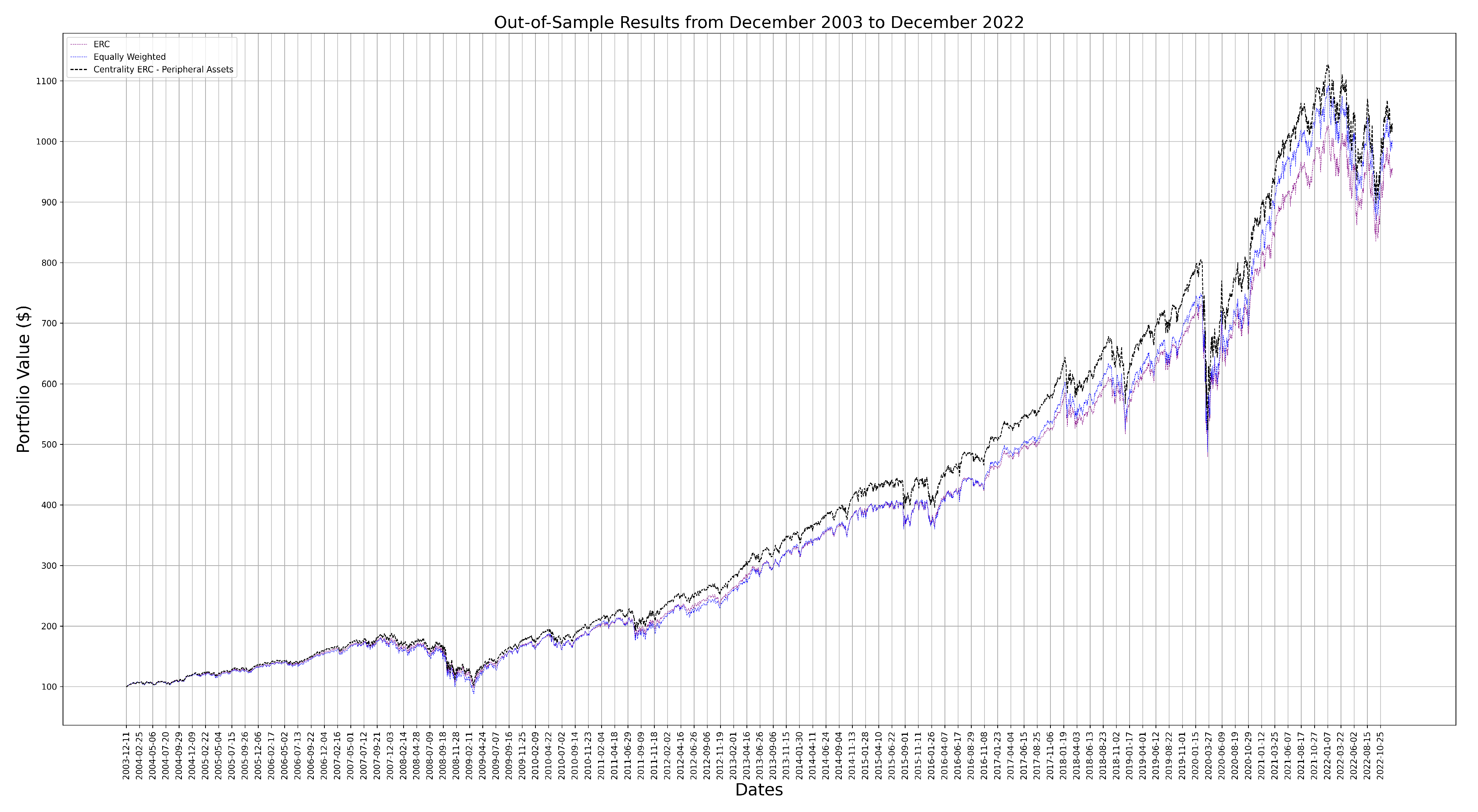
Figure 2.
Comparing Portfolio Value for Peripheral vs Central Asset Portfolios
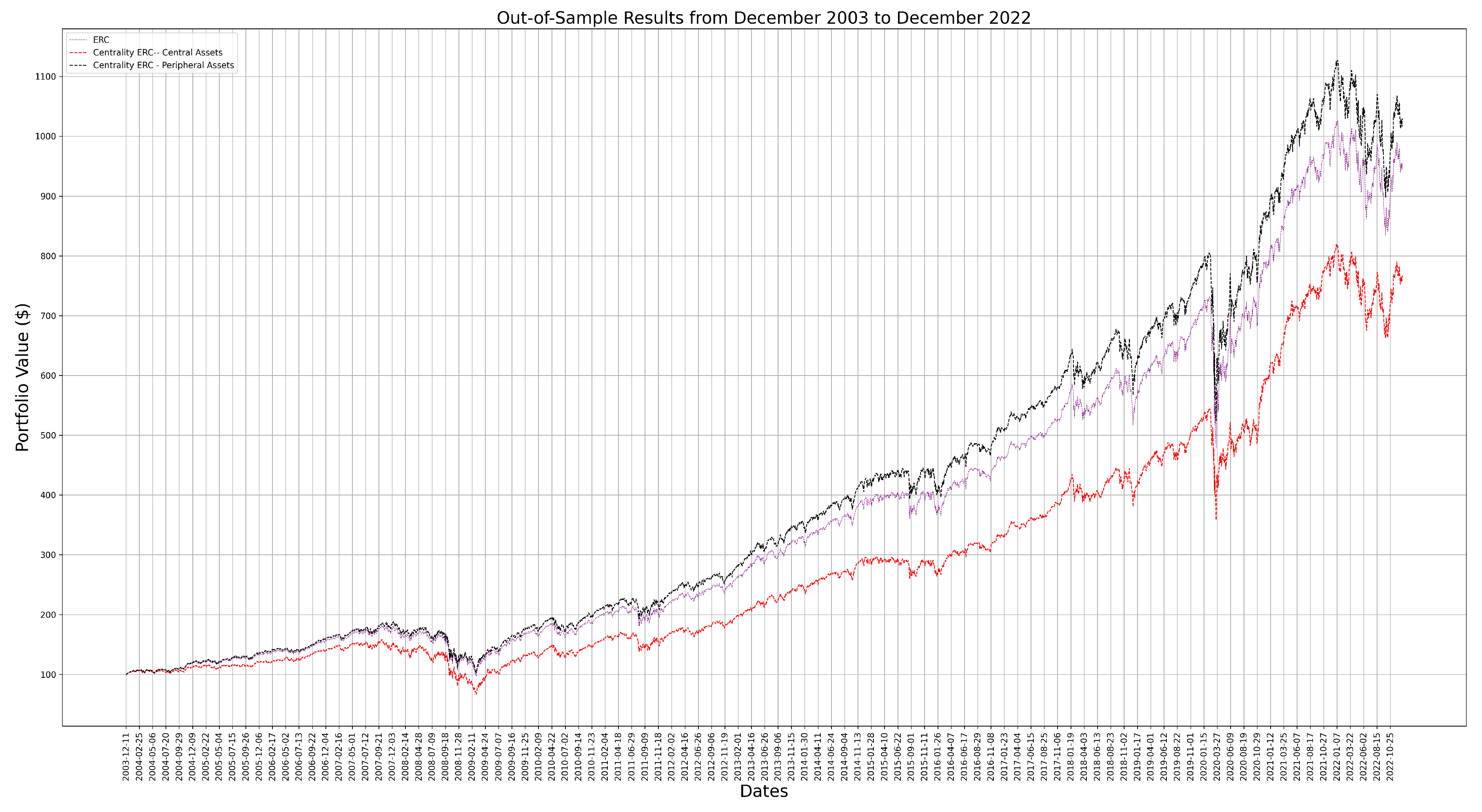
Figure 3.
ERC Weight Distribution on MST.
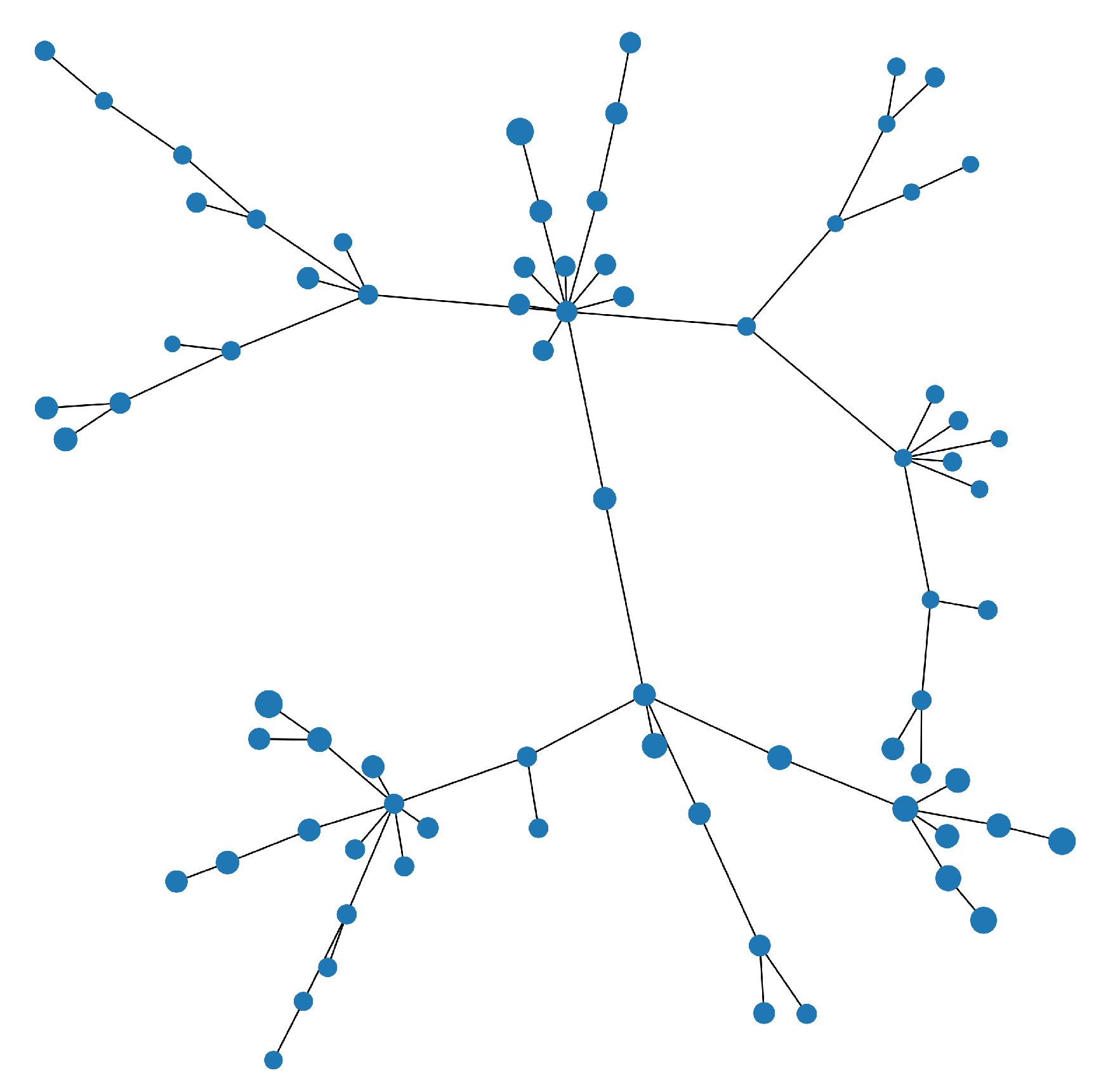
Figure 4.
Centrality ERC Weight Distribution on MST.
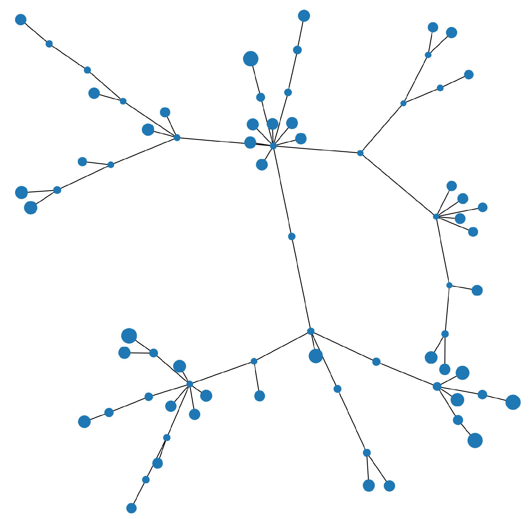
Figure 5.
MV Weight Distribution on MST.
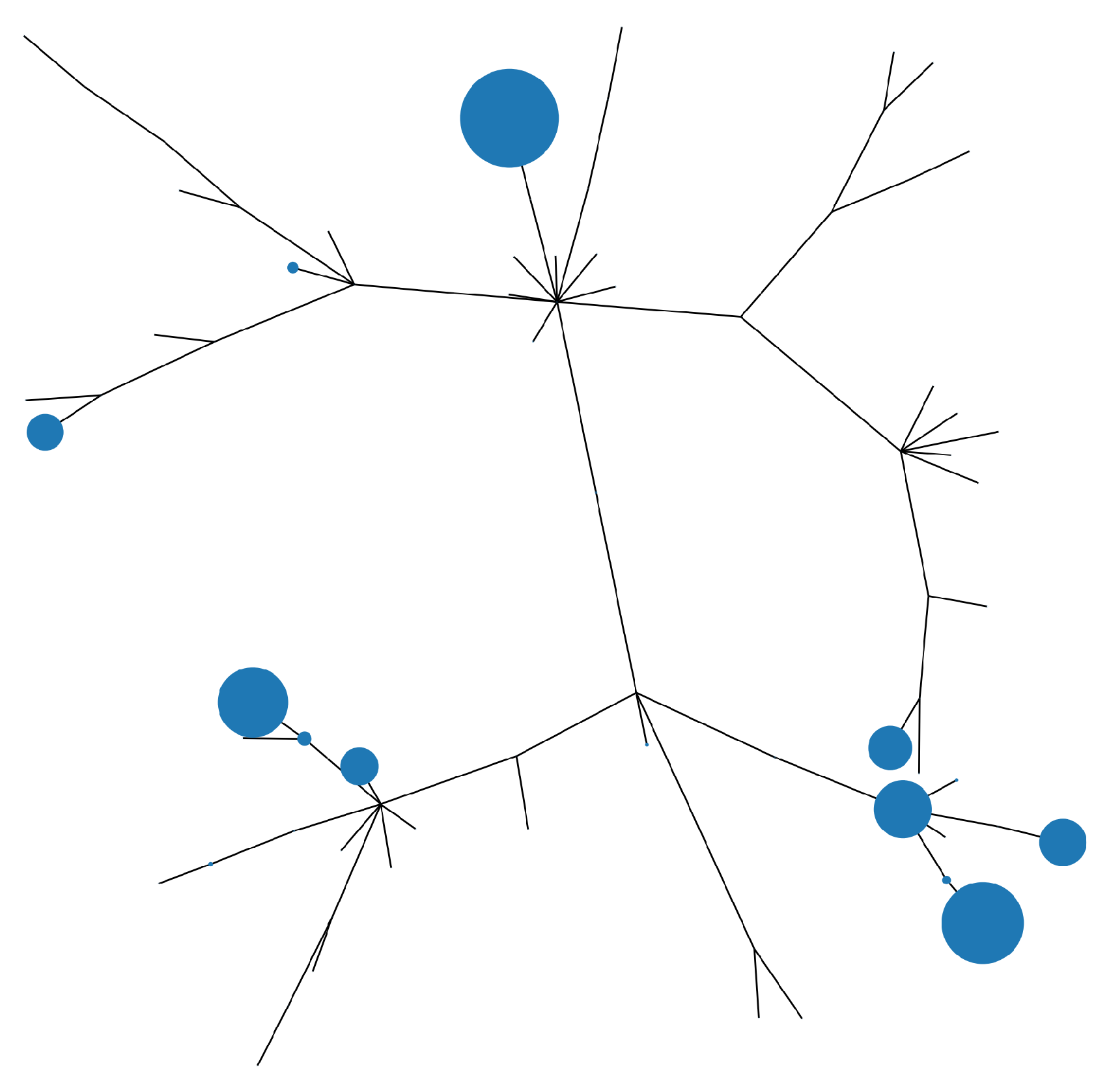
Figure 6.
Risk Contributions using Q Matrix
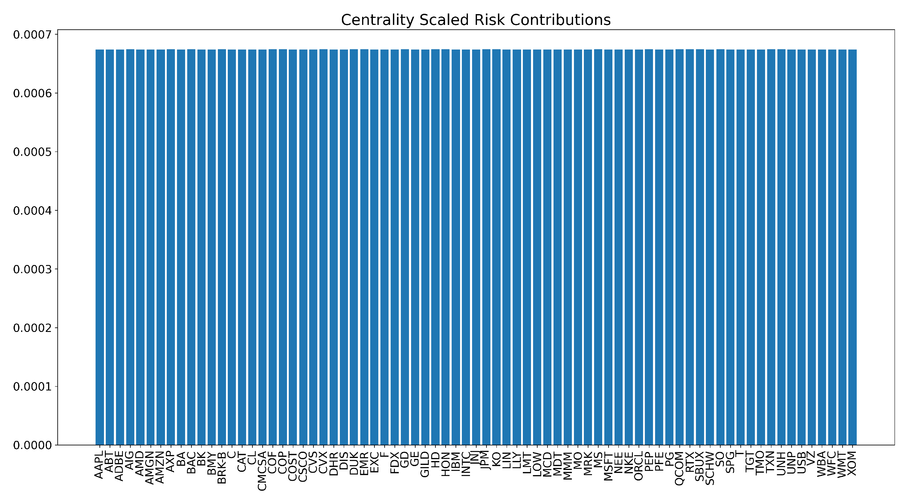
Figure 7.
Risk Contributions using Matrix
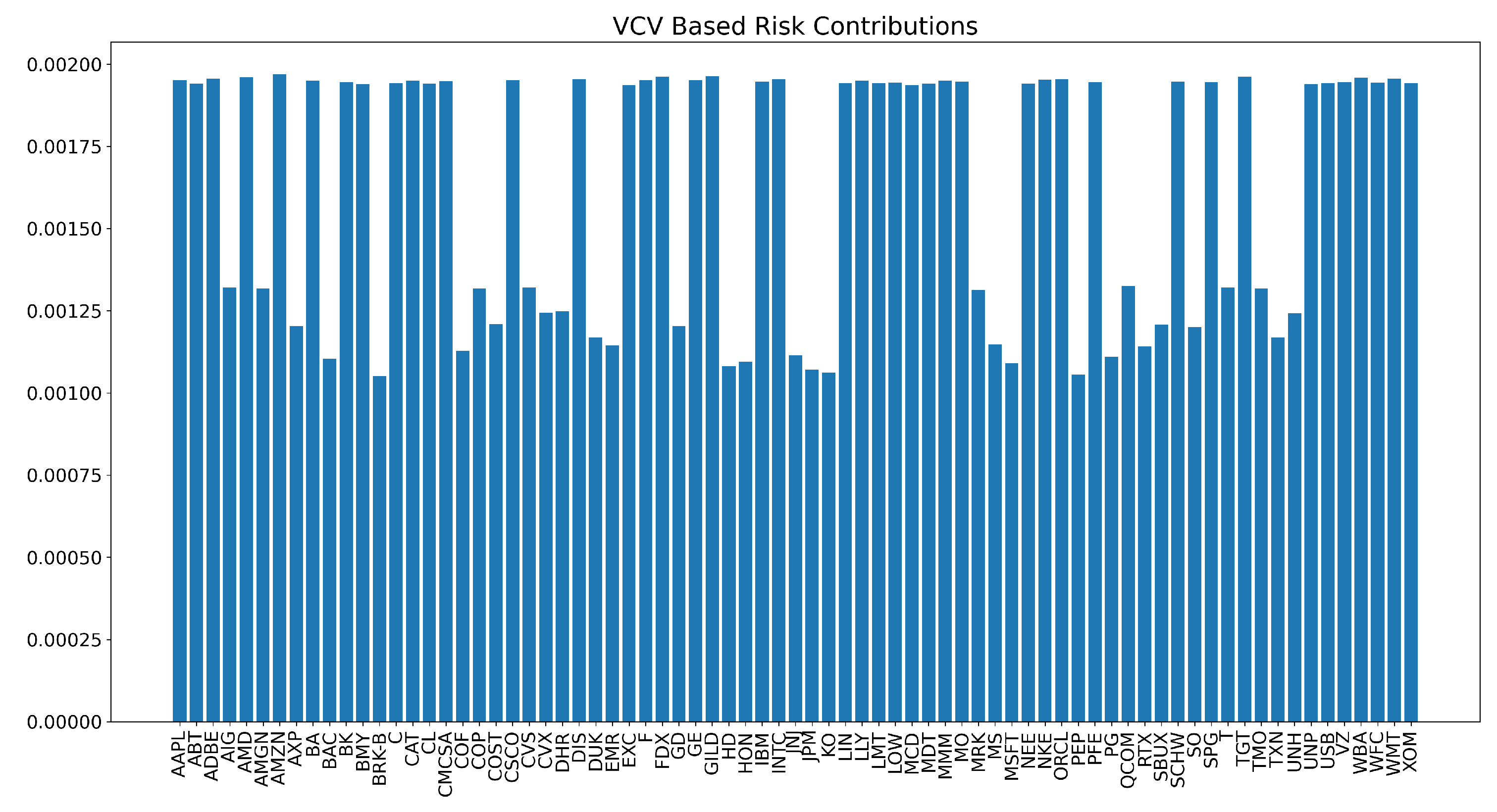

Table 1.
Summary of Literature on Network-Based Portfolios.
| Article | Traditional Portfolio Model Used | How Network Topology is Applied |
|---|---|---|
| (Peralta and Zareei 2016) | MVO (Minimize Variance objective) , MV |
|
| (Výrost et al. 2019) | MVO (Minimize Variance and Maximum Return versions) |
|
| (Giudici et al. 2022) | MVO |
|
| (Clemente et al. 2021) and (Clemente et al. 2022) | MVO (Minimum Variance-Maximum Return Dual Objective), MV, ERC, Maximum Diversification |
|
| (Baitinger and Papenbrock 2017) | MV, MVO (Minimum Variance/centrality - Maximum Return Dual Objective) |
|
| (Kaya 2013) | Naïve ERC |
|
| (Cho and Song 2023) | HRP |
|
| (Zhao et al. 2018) | MVO (Minimum Variance-Maximum Return Dual Objective) and Minimum Conditional Value at Risk (CVaR) |
|
Table 2.
Portfolio performance metrics (expressed as percentage except for Sharpe Ratio)
| Portfolio | Sharpe Ratio | Annual Return | Annual Volatility | Turnover | |
|---|---|---|---|---|---|
| Centrality ERC | 0.62 | 13.02 | 17.64 | 6.80 | 16.32 |
| ERC | 0.59 | 12.58 | 17.72 | 6.31 | 5.10 |
| EW | 0.57 | 12.86 | 19.28 | 6.02 | - |
Table 3.
Downside Risk Measures: Bear Market Sub-periods (expressed as percentage)
| 2008 | ||||||||
| Portfolio | % | MDD | % MDD | VaR | % VaR | CVaR | % CVaR | |
| Centrality ERC | -34.16 | -3.43 | 45.64 | -1.65 | -3.8030 | -2.71 | -5.2671 | -1.49 |
| ERC | -35.38 | 0 | 46.41 | 0 | -3.9091 | 0 | -5.3466 | 0 |
| EW | -39.12 | 10.59 | 50.76 | 9.38 | -4.5743 | 17.02 | -5.9498 | 11.28 |
| 2020 | ||||||||
| Centrality ERC | -59.06 | 1.94 | 34.85 | 1.18 | -5.2072 | -2.32 | -8.8003 | 1.85 |
| ERC | -57.93 | 0 | 34.44 | 0 | -5.3307 | 0 | -8.6404 | 0 |
| EW | -60.83 | 5.00 | 34.94 | 1.46 | -5.3910 | 1.13 | -8.8424 | 2.34 |
Table 4.
Varying the Look-back and Out-of-Sample Period Lengths
| Look-back Length | Out-of-sample Length | Centrality ERC Sharpe | ERC Sharpe | Centrality ERC Sharpe (Shrinkage) |
|---|---|---|---|---|
| 2 | 1 | 0.60 | 0.59 | 0.60 |
| 2 | 3 | 0.60 | 0.59 | 0.60 |
| 2 | 6 | 0.60 | 0.59 | 0.60 |
| 2 | 12 | 0.61 | 0.59 | 0.61 |
| 3 | 1 | 0.61 | 0.60 | 0.61 |
| 3 | 3 | 0.62 | 0.60 | 0.62 |
| 3 | 6 | 0.62 | 0.59 | 0.62 |
| 3 | 12 | 0.62 | 0.59 | 0.62 |
| 5 | 1 | 0.63 | 0.60 | 0.63 |
| 5 | 3 | 0.63 | 0.60 | 0.63 |
| 5 | 6 | 0.63 | 0.60 | 0.63 |
| 5 | 12 | 0.62 | 0.60 | 0.62 |
Table 5.
Downside Risk Measures: Bear Market Sub-periods with Shrinkage, expressed as percentage
| 2008 | ||||||||
| Portfolio | % | MDD | % MDD | VaR | % VaR | CVaR | % CVaR | |
| Centrality ERC | -34.18 | -3.43 | 45.65 | -1.67 | -3.806 | -2.64 | -5.269 | -1.49 |
| ERC | -35.39 | 0 | 46.42 | 0 | -3.909 | 0 | -5.348 | 0 |
| EW | -39.12 | 10.55 | 50.76 | 9.34 | -4.574 | 17.01 | -5.950 | 11.24 |
| 2020 | ||||||||
| Centrality ERC | -59.07 | 1.93 | 34.85 | 1.18 | -5.208 | -2.32 | -8.801 | 1.85 |
| ERC | -57.95 | 0 | 34.44 | 0 | -5.331 | 0 | -8.641 | 0 |
| EW | -60.83 | 4.96 | 34.94 | 1.46 | -5.391 | 1.12 | -8.842 | 2.33 |
Disclaimer/Publisher’s Note: The statements, opinions and data contained in all publications are solely those of the individual author(s) and contributor(s) and not of MDPI and/or the editor(s). MDPI and/or the editor(s) disclaim responsibility for any injury to people or property resulting from any ideas, methods, instructions or products referred to in the content. |
© 2023 by the authors. Licensee MDPI, Basel, Switzerland. This article is an open access article distributed under the terms and conditions of the Creative Commons Attribution (CC BY) license (http://creativecommons.org/licenses/by/4.0/).
Copyright: This open access article is published under a Creative Commons CC BY 4.0 license, which permit the free download, distribution, and reuse, provided that the author and preprint are cited in any reuse.


