Submitted:
30 November 2023
Posted:
30 November 2023
You are already at the latest version
Abstract
Keywords:
1. Introduction
2. Related Works
3. Model Construction
3.1. Adaptive Graph Convolution Module
3.2. Global Attention
3.3. A 3D Point Cloud Classification Method Based on Adaptive Graph Convolution and Attention
4. Experimental Results and Analysis
4.1. Datasets
4.2. Experimental Environment and Parameter Configuration
4.3. Analysis of different ‘k’ values
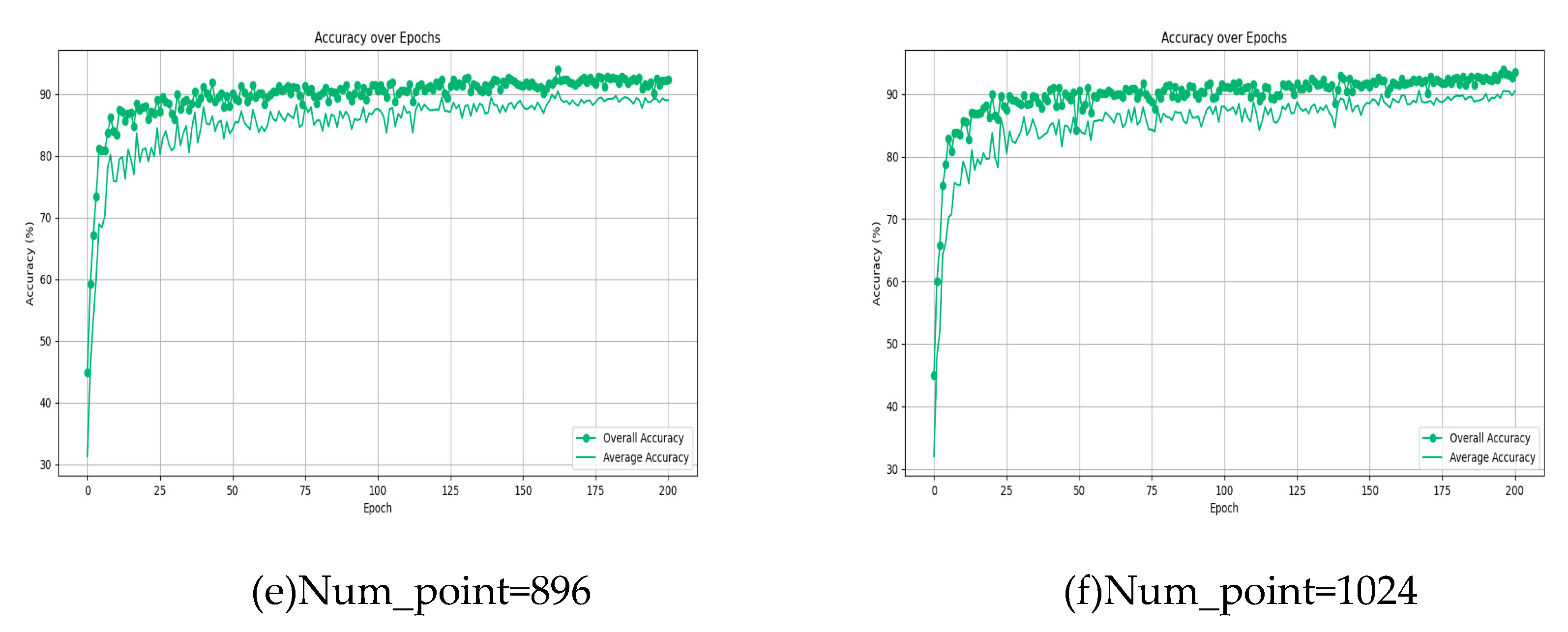
4.3. Analysis of different point cloud numbers
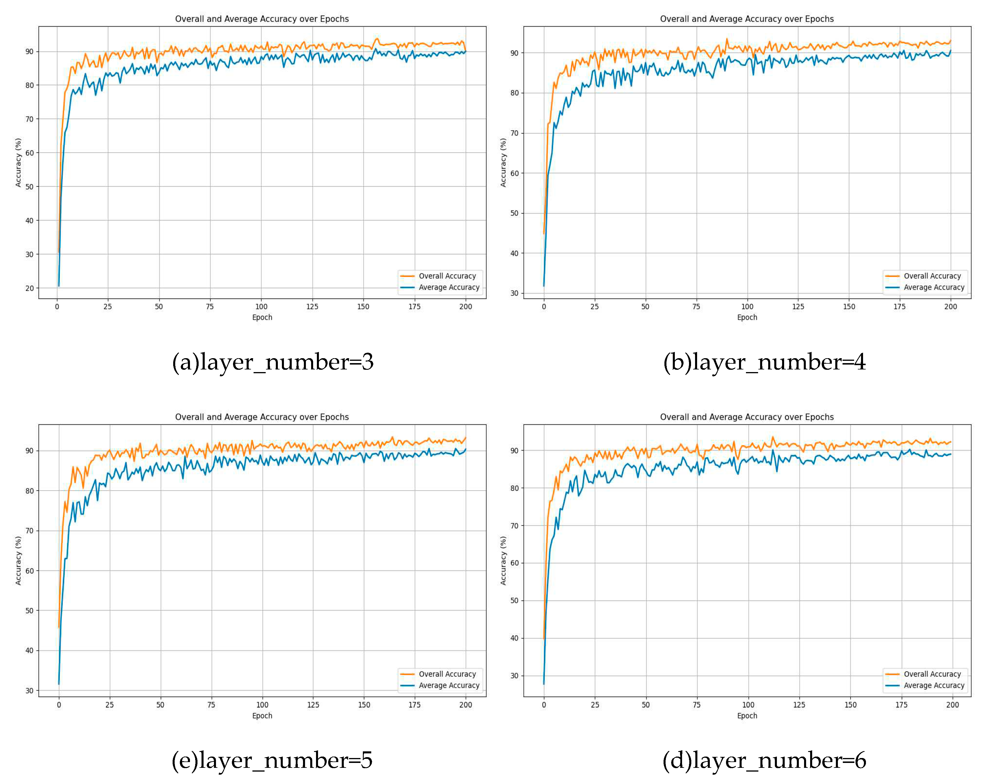
4.4. The Impact of Perceptron Layer Depth on Model Performance
4.5. Effectiveness of the Proposed Algorithm in 3D Point Cloud Classification
- (1)
- PointNet: It is comprised of Multi-Layer Perceptrons (MLPs), max pooling layers, and fully connected layers, capable of directly processing point clouds and extracting spatial features for classification tasks.
- (2)
- PointNet++: It is an advanced model that builds upon the original PointNet architecture, introducing hierarchical neural networks and utilizing a set abstraction layer to capture local structures at multiple scales, enabling more effective processing of spatially distributed data in point clouds.
- (3)
- PCNN: The framework consists of two operators: extension and restriction, mapping point cloud functions to volumetric functions and vise-versa. A point cloud convolution is defined by pull-back of the Euclidean volumetric convolution via an extension-restriction mechanism.
- (4)
- GGM-Net: The central component of GGM-Net revolves around extracting features through geometric moments, a process known as GGM convolution. This method involves learning point-specific features and local characteristics from the first and second-order geometric moments of a point and its immediate neighbors. These learned features are then integrated using an additive approach.
- (5)
- GAPNet: Local geometric representations are learned by embedding a graph attention mechanism within stacked MLPs layers.
- (6)
- FatNet: Presents a new neural network layer, known as the FAT layer, designed to integrate both global point-based and local edge-based features, thereby producing more effective embedding representations.
- (7)
- CT-BLOCK: In the CT-block, two distinct branches are integrated: the 'C' branch, signifying the convolution aspect, and the 'T' branch, representing the transformer aspect. The convolution branch focuses on executing convolutions on gathered neighboring points to derive local features. Concurrently, the transformer branch applies an offset-attention mechanism to the entire point cloud, facilitating the extraction of global features.
- (8)
- DI-PointCNN: The feature extractor obtains high-dimensional features, while the feature comparator aggregates and disperses homogenous and heterogeneous point clouds in the feature space, respectively. The feature analyzer then completes the task.
- (9)
- DGCNN: A novel neural network module named EdgeConv is proposed, which incorporates local neighborhood information and can be stacked to learn global shape attributes. In a multi-layered system, the affinities in the feature space capture semantic features that may span long distances in the original embeddings.
- (10)
- AGCNN: A graph-based neural network with an attention pooling strategy, termed AGNet, is proposed, capable of extracting local feature information through the construction of topological structures.
- (11)
- Point-Transformer: The Point Transformer model introduces dot-product and point convolution operations, overcoming the limitations of traditional 3D CNNs in processing point cloud data, and offers enhanced flexibility and scalability.
- (12)
- UFO-Net: An efficient local feature learning module is employed as a bridging technique to connect diverse feature extraction modules. UFO-Net utilizes multiple stacked blocks to better capture the feature representations of point clouds.
- (13)
- APES: An attention-based, non-generative point cloud edge sampling method (APES), inspired by the image Canny edge detection algorithm and aided by attention mechanisms.
- (14)
- ULIP+PointNet++: ULIP employs a pre-trained visual-language model, which has already learned a common visual and textual space through extensive training on a vast number of image-text pairs. Subsequently, ULIP utilizes a small set of automatically synthesized triplets to learn a 3D representation space aligned with the public image-text space.
| model | Accuracy | |
| Avearge accuracy | Overall accuracy | |
| PointNet[1] | 86.2 | 89.2 |
| PointNet++[2] | - | 91.9 |
| PCNN[4] | 88.1 | 92.2 |
| GGM-Net[27] | 89.0 | 92.6 |
| GAPNet[25] | 89.7 | 92.4 |
| FatNet[32] | 90.6 | 93.2 |
| CT-BLOCK[33] | 90.8 | 93.5 |
| DI-PointCNN[34] | 88.3 | 92.1 |
| DGCNN[35] | 90.2 | 92.9 |
| AGCNN[36] | 90.7 | 93.4 |
| Point-Transformer[11] | 90.6 | 93.7 |
| UFONet[37] | 90.8 | 93.7 |
| APES[38] | - | 93.5 |
| ULIP+PointNet++[39] | - | 93.4 |
| Att-AdaptNet(ours) | 90.8 | 93.8 |
4.6. The Effects of Various Attention Mechanisms
5. Conclusions
Author Contributions
Funding
Data Availability Statement
Conflicts of Interest
References
- Charies, R.; Hao, S.; Kaichun, M.; Leonidas, J. PointNet: Deep Learning on Point Sets for 3D Classification and Segmentation. Proceedings of the IEEE Conference on Computer Vision and Pattern Recognition (CVPR), Hawaii, United States, July 2017; pp. 652-660. [CrossRef]
- Charles, R.; Li, Y.; Hao, S.; Leonidas, J. PointNet++: Deep Hierarchical Feature Learning on Point Sets in a Metric Space. arXiv: 2017, arXiv: 1706.02413. [CrossRef]
- Charies, R.; Wei, L.; Chenxia, W.; Hao, S.; Leonidas, J. Frustum pointnets for 3d object detection from rgb-d data .Proceedings of the IEEE Conference on Computer Vision and Pattern Recognition (CVPR), Salt Lake City, United States, June 2018; pp. 918-927. [CrossRef]
- Atzmon, M.; Maron, H.; Lipman, Y. Point convolutional neural networks by extension operators. arXiv: 2018, arXiv: 1803.10091. [CrossRef]
- Wang, Y.; Sun, Y.; Liu, Z. Dynamic graph cnn for learning on point clouds. ACM TOG. 2019, 38(5): 1-12. [CrossRef]
- Zhao, H.; Jiang, L.; Fu, C. Pointweb: Enhancing local neighborhood features for point cloud processing. Proceedings of the IEEE/CVF Conference on Computer Vision and Pattern Recognition, California, Los Angeles, June 2019; pp. 5565-5573. [CrossRef]
- Zhang, M.; You, H.; Kadam, P. Pointhop: An explainable machine learning method for point cloud classification. IEEE. TMM. 2020, 22(7): 1744-1755. [CrossRef]
- Ben-Shabat, Y.; Lindenbaum, M.; Fischer, A. 3dmfv: Three-dimensional point cloud classification in real-time using convolutional neural networks. IEEE. RA-L. 2018, 3(4): 3145-3152. [CrossRef]
- Zhao, Y.; Birdal, T.; Deng, H. 3D point capsule networks. Proceedings of the IEEE/CVF Conference on Computer Vision and Pattern Recognition(CVPR), California, Los Angeles, June 2019; pp. 1009-1018. [CrossRef]
- Vaswani, A.; Shazeer, N.; Parmar, N. Attention is all you need. Advances in Neural Information Processing Systems, Long Beach, CA, USA, Jun 2017; pp. 5998-6008. [CrossRef]
- Wang, X.; Zhang, W.; Li, C.; Xiong, Z.; Xu, M. Point Transformer: A Versatile Framework for 3D Point Cloud Analysis. IEEE International Conference on Computer Vision(ICCV), Online, October 2021; pp. [CrossRef]
- He, K. Point cloud transformer: A deep learning framework for 3D point cloud analysis. arXiv, 2018; arXiv:1812.04419. [Google Scholar]
- Fujiwara, K.; Hashimoto, T. Neural implicit embedding for point cloud analysis. Proceedings of the IEEE/CVF Conference on Computer Vision and Pattern Recognition, Online, June 2020; pp. 11734-11743. [CrossRef]
- Hamilton, W.; Ying, R.; Leskovec, J. Inductive representation learning on large graphs. Proceedings of the 31st International Conference on Neural Information Processing Systems, California, Los Angeles, December 2017; pp. 1025-1035. [CrossRef]
- Lin, Z.; Huang, S.; Wang, Y. Convolution in the cloud: Learning deformable kernels in 3d graph convolution networks for point cloud analysis. Proceedings of the IEEE/CVF Conference on Computer Vision and Pattern Recognition, California, Seattle, June 2020; pp.1800-1809. [CrossRef]
- Wang, L.; Huang, Y.; Hou, Y. Graph attention convolution for point cloud semantic segmentation. Proceedings of the IEEE/CVF Conference on Computer Vision and Pattern Recognition(CVPR), California, Los Angeles, June 2019; pp. 10296-10305. [CrossRef]
- Zhang, W.; Xiao, C. PCAN: 3D attention map learning using contextual information for point cloud based retrieval. Proceedings of the IEEE/CVF Conference on Computer Vision and Pattern Recognition(CVPR), California, Los Angeles, June 2019; pp. 12436-12445. [CrossRef]
- Lan, S.; Yu, R.; Yu, G. Modeling local geometric structure of 3d point clouds using geo-cnn. Proceedings of the IEEE/CVF Conference on Computer Vision and Pattern Recognition(CVPR), California, Los Angeles, June 2019; pp. 998-1008. [CrossRef]
- Liu, Y.; Fan, B.; Xiang, S. Relation-shape convolutional neural network for point cloud analysis. Proceedings of the IEEE/CVF Conference on Computer Vision and Pattern Recognition(CVPR), California, Los Angeles, June 2019; pp. 8895-8904. [CrossRef]
- Kelvin, X.;Jimmy, Ba.;Ryan, K.; Show, Attend and Tell: Neural Image Caption Generation with Visual Attention. Proceedings of the 32nd International Conference on Machine Learning, Lyon, Frence, July 2015; pp. 2048-2057. [CrossRef]
- Bahdanau, D.; Chorowski, J.; Serdyuk, D. End-to-end attention-based large vocabulary speech recognition. 2016 IEEE international conference on acoustics, speech and signal processing (ICASSP), Las Vegas, Nevada, March 2016; pp. 4945-4949. [CrossRef]
- Xu, T.; Zhang, P.; Huang, Q. Attngan: Fine-grained text to image generation with attentional generative adversarial networks. Proceedings of the IEEE conference on computer vision and pattern recognition, Salt Lake City, Utah, June 2018; pp. 1316-1324. [CrossRef]
- Hu, J.; Shen, L.; Sun, G. Squeeze-and-excitation networks. Proceedings of the IEEE conference on computer vision and pattern recognition, Salt Lake City, Utah, June 2018; pp. 7132-7141. [CrossRef]
- Petar, V.; Guillem, C.; Arantxa, C.; Adriana R.; Pietro, L.; Yoshua, B. Graph Attention Networks. stat, 2017,1050(20), pp.10-48550. [CrossRef]
- Chen, C.; Fragonara, L.; Tsourdos, A. GAPNet: Graph attention based point neural network for exploiting local feature of point cloud. arXiv, 2019; arXiv:1905.08705. [Google Scholar]
- Yang, J.; Zhang, Q.; Ni, B.; et al. Modeling point clouds with self-attention and gumbel subset sampling. Proceedings of the IEEE/CVF conference on computer vision and pattern recognition(CVPR), California, Los Angeles, June 2019; pp. 3323-3332.
- Li, D.; Shen, X.; Yu, Y.; et al. GGM-net: Graph geometric moments convolution neural network for point cloud shape classification. IEEE Access. 2020, 8: 124989-124998. [CrossRef]
- Li, R.; Wang, S.; Zhu, F. Adaptive graph convolutional neural networks. Proceedings of the AAAI Conference on Artificial Intelligence, California, Newport Beach, February 2018.
- Li H, Xiong P, An J, et al. Pyramid attention network for semantic segmentation. arXiv: 2018, arXiv: 1805.10180. [CrossRef]
- Zhiheng, K.; Ning, L. PyramNet: Point cloud pyramid attention network and graph embedding module for classification and segmentation. ArXiv:2019, arXiv:1906.03299. [CrossRef]
- Li, X.; Wang, W.; Hu, X. Selective kernel networks, Proceedings of the IEEE/CVF Conference on Computer Vision and Parttern Recognition, Los Angeles CA, United States, June 2019; pp. 510-519.
- Kaul, C.; Pears, N.; Manandhar, S. FatNet: A feature-attentive network for 3D point cloud processing. 2020 25th International Conference on Pattern Recognition (ICPR), Milan, Italy, January 2020; pp. 7211-7218.
- Guo, S.; Li, J.; Lai, Z.; et al. CT-block: a novel local and global features extractor for point cloud. arXiv: 2021, arXiv: 2111.15400. [CrossRef]
- Zhai, R.; Li, X.; Wang, Z.; et al. Point cloud classification model based on a dual-input deep network framework. IEEE Access. 2020, 8:55991-55999. [CrossRef]
- Wang, Y.; Sun, Y.; Liu, Z.; Sarma, S.E.; Bronstein, M.M.; Solomon, J.M. Dynamic graph CNN for learning on point clouds. ACM Trans. Graph. 2019, 38, 146. [Google Scholar] [CrossRef]
- Jing, W.; Zhang, W.; Li, L.; Di, D.; Chen, G.; Wang, J. AGNet: An attention-based graph network for point cloud classification and segmentation. Remote Sens. 2022, 14, 1036. [Google Scholar] [CrossRef]
- He, S.; Guo, P.; Tang, Z.; Guo, D.; Wan, L.; Yao, H. UFO-Net: A Linear Attention-Based Network for Point Cloud Classification. Sensors. 2023, 23, 5512. [Google Scholar] [CrossRef] [PubMed]
- Wu, C.; Zheng, J.; Julius P.; Jürgen B. Attention-based Point Cloud Edge Sampling. Proceedings of the IEEE/CVF Conference on Computer Vision and Pattern Recognition (CVPR), Vancouver, Canada, June 2023, pp. 5333-5343.
- Xue L.; Gao M.; Xing C.; Roberto M.; Wu J.; Xiong C.; Xu R.; Juan C.; Silvio S. ULIP: Learning a Unified Representation of Language, Images, and Point Clouds for 3D Understanding, Proceedings of the IEEE/CVF Conference on Computer Vision and Pattern Recognition (CVPR), Vancouver, Canada ,June 2023, pp. 1179-1189.

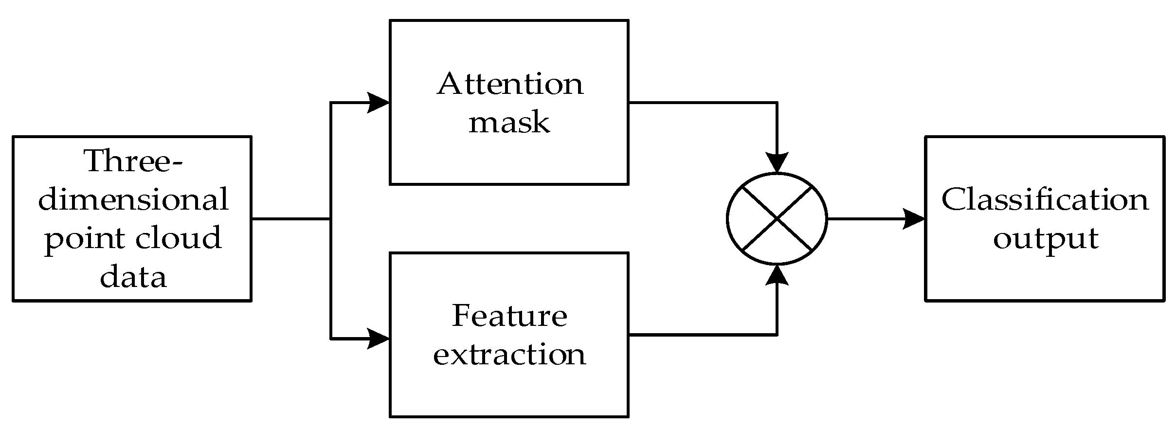


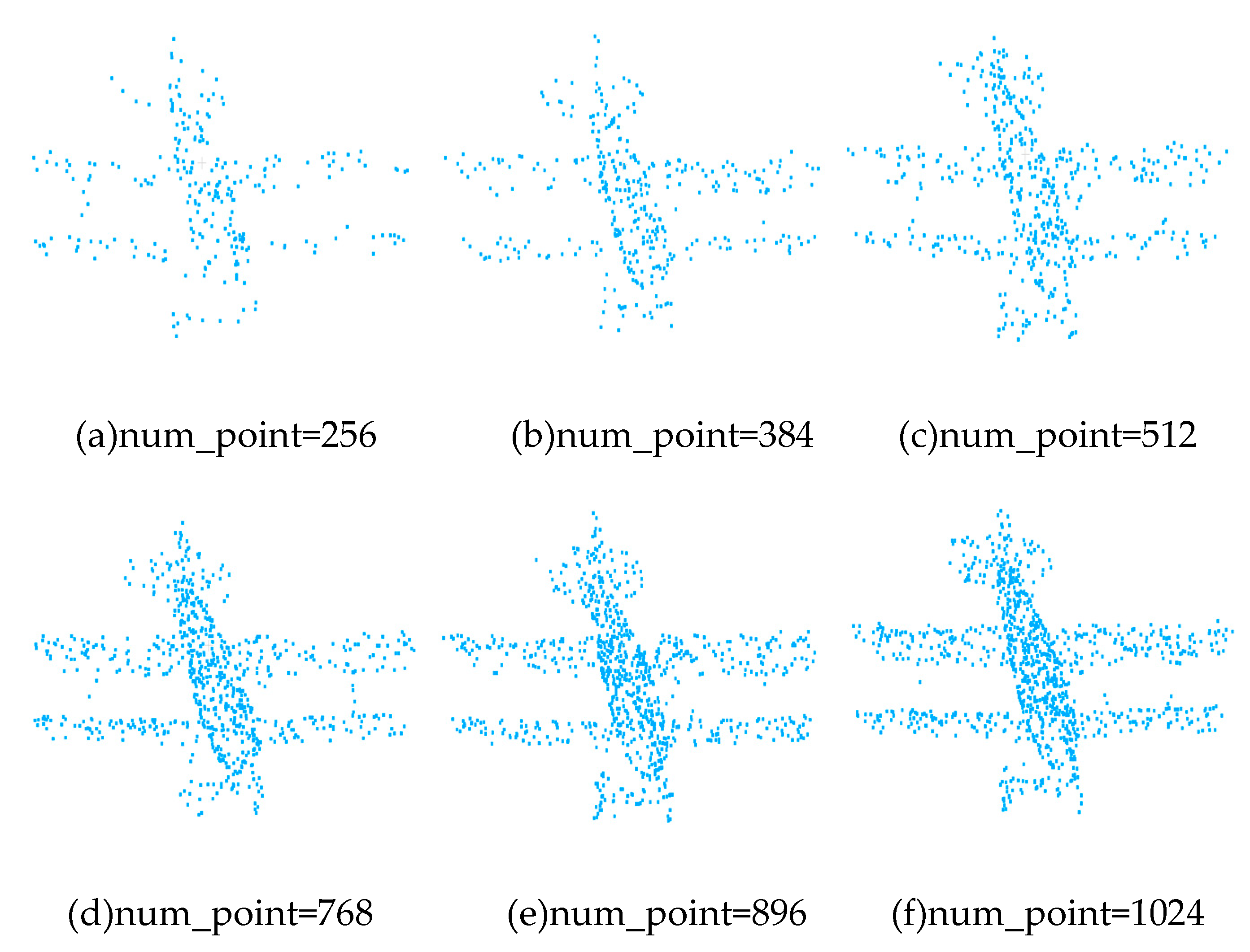
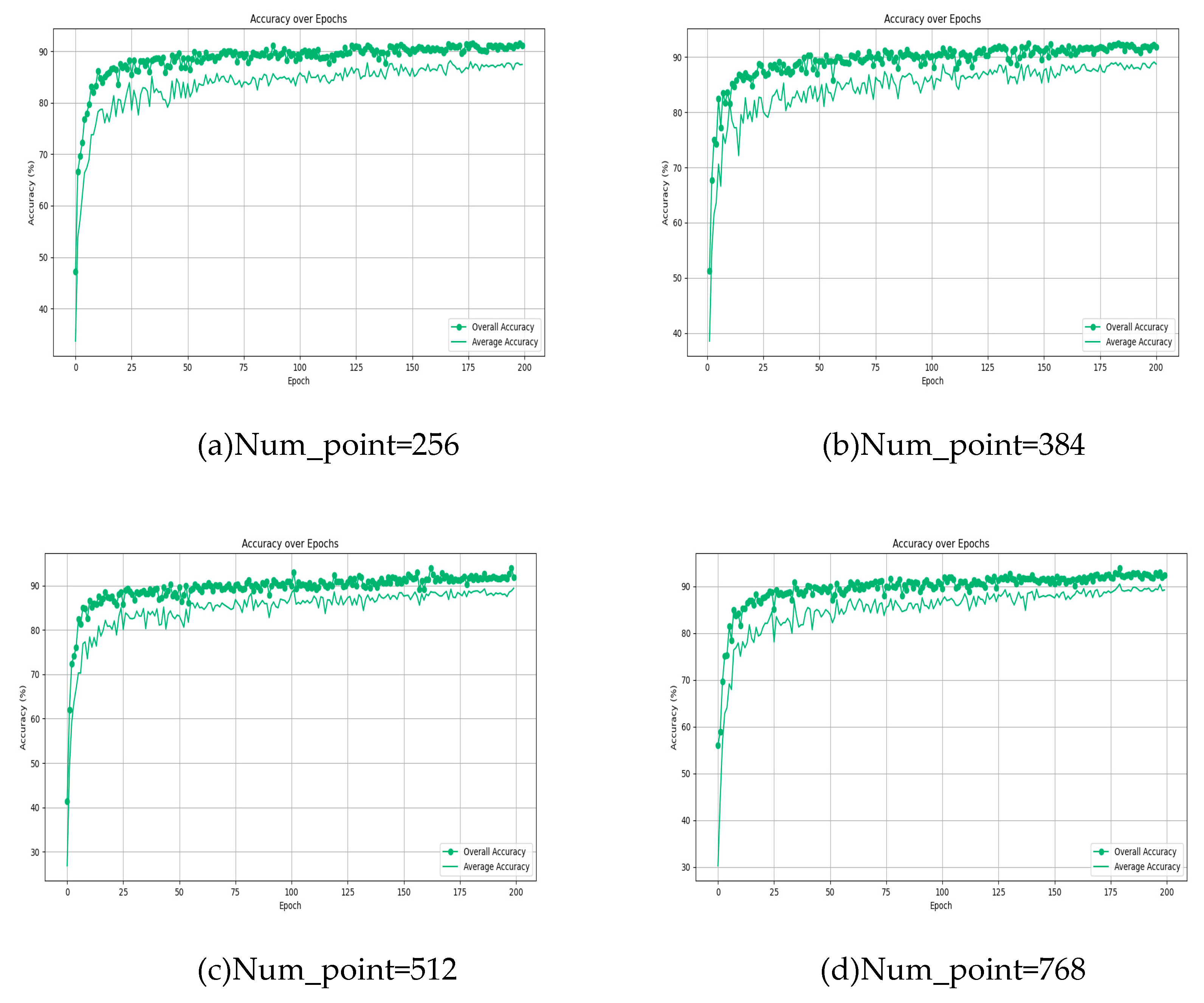
| Experimental environment | Model parameter | ||
| Enviroment | Configuration | parameter | Configuration |
| CPU | Ryzen 5 2400G | Batch size | 16 |
| GPU | NVIDIA RTX A2000 | Point cloud | 1024 |
| RAM | 12G | Max epoch | 200 |
| Operating system | Window10 | Optimizer | SGD |
| Programming Language | Python3.8 | Learning rate | 0.001 |
| Deep Learning Framework | Pytorch1.1 | Momentum | 0.9 |
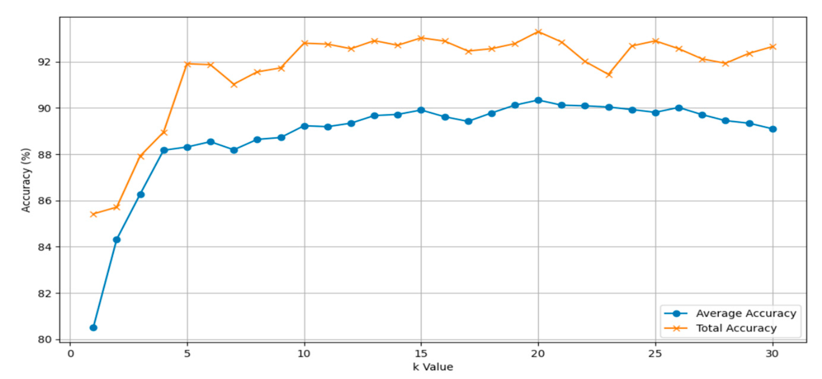
| K value | Average accuracy | Total accuracy |
| 5 | 88.31 | 91.91 |
| 10 | 89.23 | 92.80 |
| 15 | 89.91 | 93.03 |
| 20 | 90.34 | 93.32 |
| 25 | 89.81 | 92.90 |
| 30 | 89.10 | 92.65 |
| Model | Average accuracy | Total accuracy |
| AdaptNet | 90.7 | 93.4 |
| AdaptNet +Self-Attention | 90.7 | 93.5 |
| AdaptNet +MultiHead-Attention | 90.5 | 93.4 |
| Att-AdaptNet(Ours) | 90.8 | 93.8 |
Disclaimer/Publisher’s Note: The statements, opinions and data contained in all publications are solely those of the individual author(s) and contributor(s) and not of MDPI and/or the editor(s). MDPI and/or the editor(s) disclaim responsibility for any injury to people or property resulting from any ideas, methods, instructions or products referred to in the content. |
© 2023 by the authors. Licensee MDPI, Basel, Switzerland. This article is an open access article distributed under the terms and conditions of the Creative Commons Attribution (CC BY) license (http://creativecommons.org/licenses/by/4.0/).


