Submitted:
30 November 2023
Posted:
30 November 2023
You are already at the latest version
Abstract
Keywords:
1. Introduction
| Seal (zhuan): |  |
| Clerical (li): |  |
| Cursive (cao): |  |
| Semi-cursive (xing): |  |
| Regular (kai): |  |
2. Related works
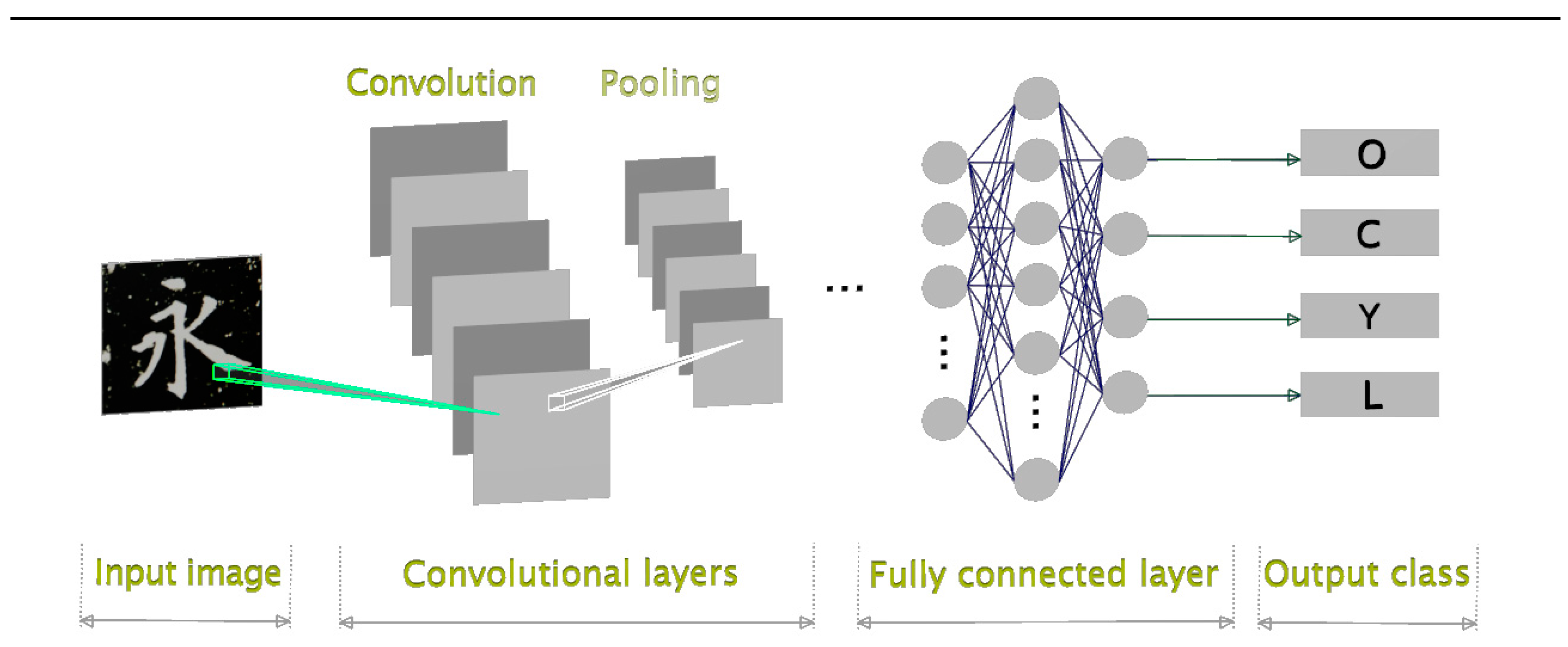
3. A CNN model for the classification of Chinese calligraphy images
 where m represents the total number of classes, yi denotes the i-th prediction class, ŷi is the i-th true class of training samples, and wi is the weight vector.
4. Experiments and Analysis
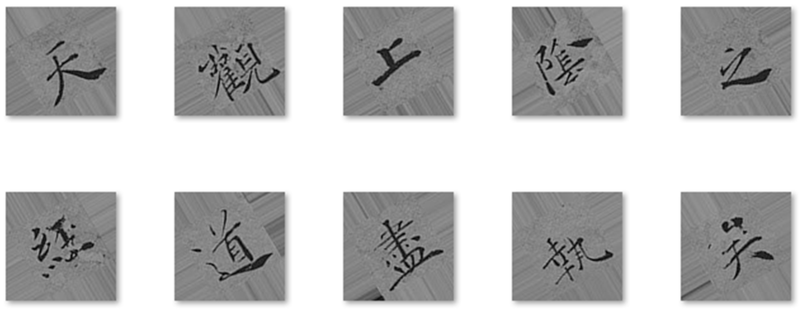
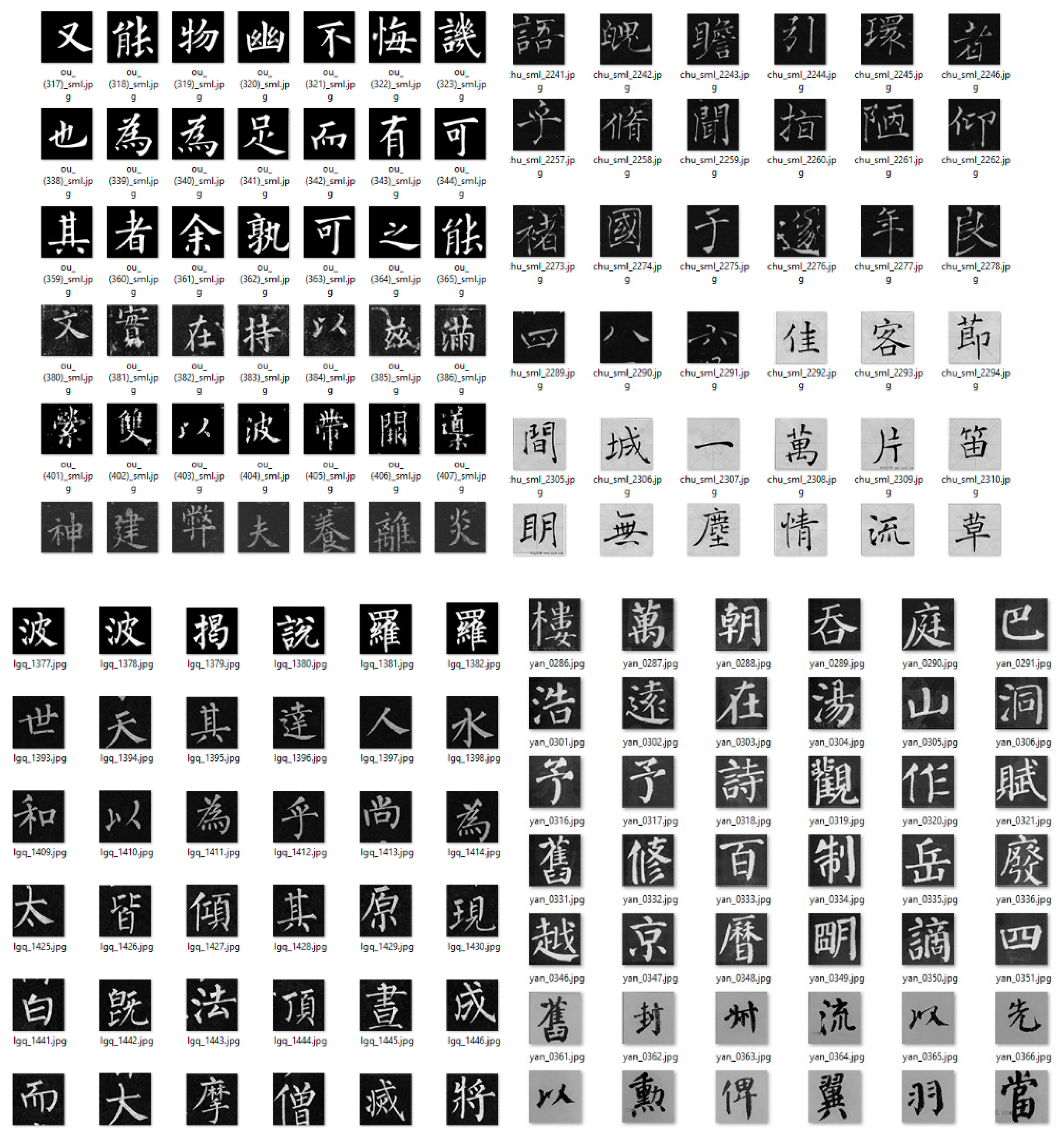
4.1. Dataset construction
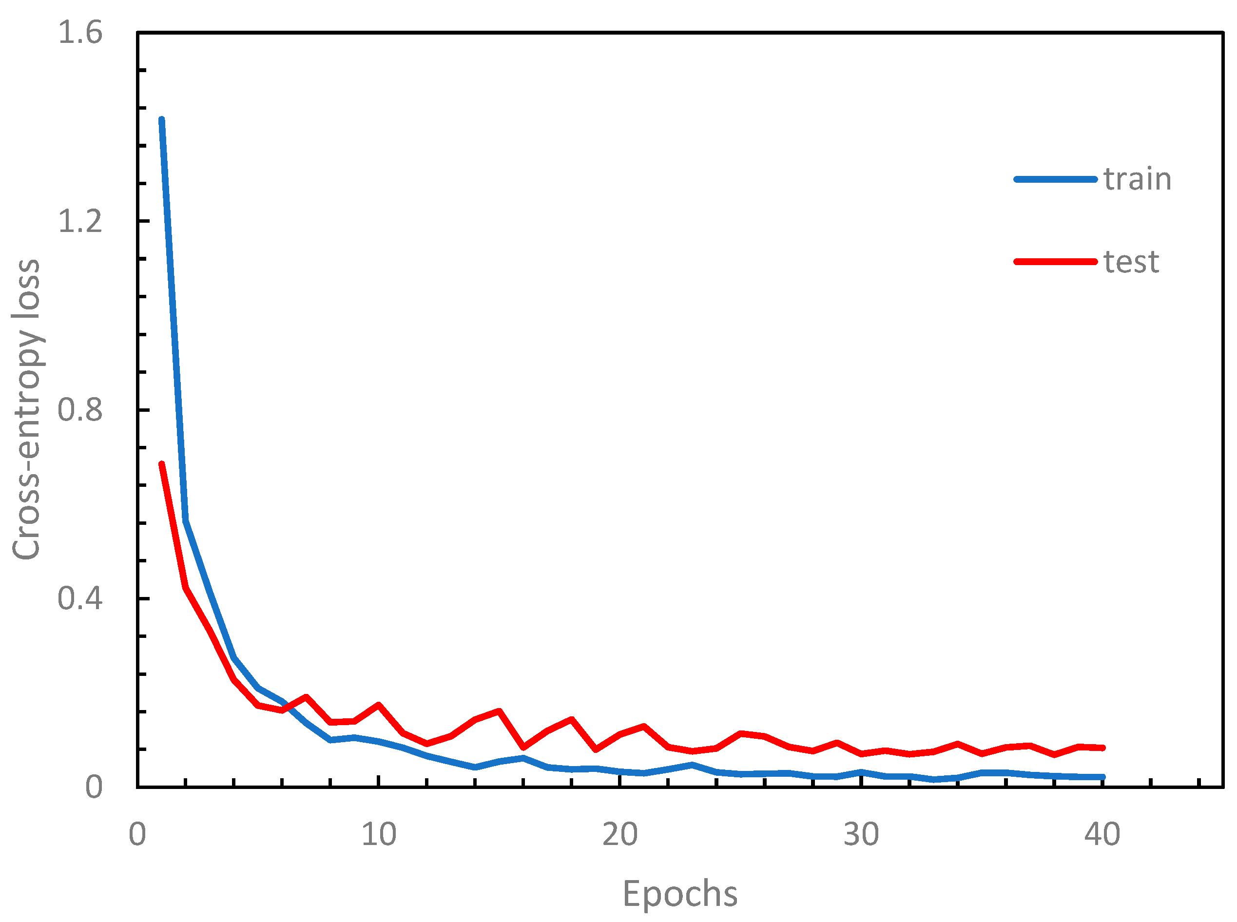
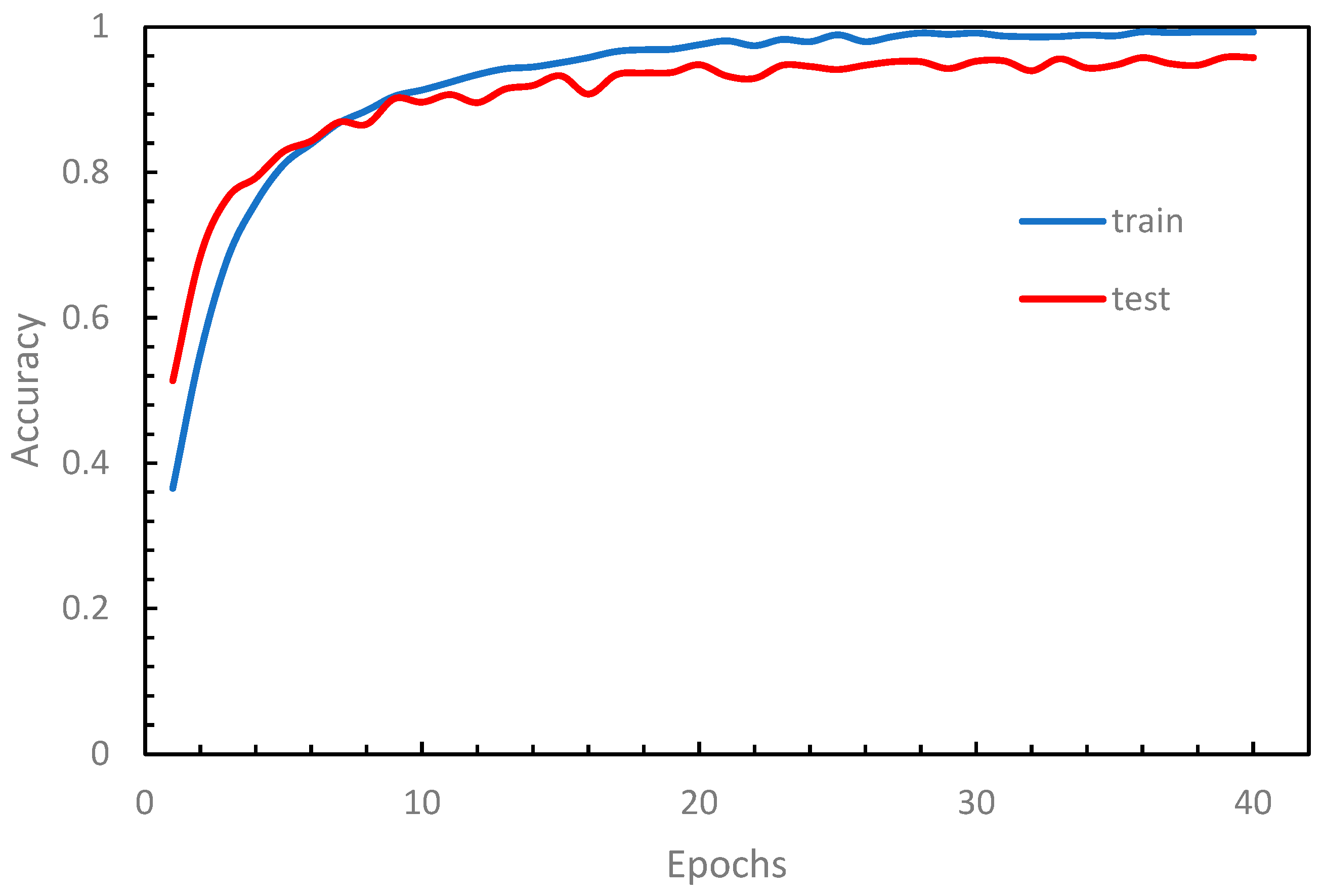
4.2. Numerical experiments, results, and discussion

| Parameters | Values |
| Input image size | 64×64×1 |
| Filter size (F×F) | 3×3, 5×5, 7×7 |
| Number of filters (K) | 16, 24, 32, 48 |
| Pooling size (Max Pooling) | 2×2 stride=2 |
| Configuration type (Cn) | C1, C2, C3, C4, C5 |
| Neuron numbers of FC Layer (N) |
512, 256, 128 |
| (1) Filter size 3×3 (K=32) | |||
| Block | Layer | Layer type |
Description (feature map size) |
| Block 1 | L1 | Conv+ReLU | 32@62×62 |
| L2 | Max Pooling | 32@31×31 | |
| Block 2 | L3 | Conv+ReLU | 64@29×29 |
| L4 | Max Pooling | 64@14×14 | |
| Block 3 | L5 | Conv+ReLU | 128@12×12 |
| L6 | Max Pooling | 128@6×6 | |
| Block 4 | L7 | Conv+ReLU | 256@4×4 |
| L8 | Max Pooling | 256@2×2 | |
| Block 5 (FC layers) |
L9 | FC1 | 512 neurons |
| L10 | FC2 | 256 neurons | |
| L11 | FC3 (softmax) | 4 neurons | |
| (2) Filter size 5×5 (K=32) | |||
| Block | Layer | Layer type |
Description (feature map size) |
| Block 1 | L1 | Conv+ReLU | 32@60×60 |
| L2 | Max Pooling | 32@30×30 | |
| Block 2 | L3 | Conv+ReLU | 64@26×26 |
| L4 | Max Pooling | 64@13×13 | |
| Block 3 | L5 | Conv+ReLU | 128@9×9 |
| L6 | Max Pooling | 128@4×4 | |
| Block 4 (FC layers) |
L7 | FC1 | 512 neurons |
| L8 | FC2 | 256 neurons | |
| L9 | FC3 (softmax) | 4 neurons | |
| (3) Filter sizes 5×5, 3×3 (K=32) | |||
| Block | Layer | Layer type |
Description (feature map size) |
| Block 1 | L1 | Conv+ReLU | 32@60×60 |
| L2 | Max Pooling | 32@30×30 | |
| Block 2 | L3 | Conv+ReLU | 64@28×28 |
| L4 | Max Pooling | 64@14×14 | |
| Block 3 | L5 | Conv+ReLU | 128@12×12 |
| L6 | Max Pooling | 128@6×6 | |
| Block 4 | L7 | Conv+ReLU | 256@4×4 |
| L8 | Max Pooling | 256@2×2 | |
| Block 5 (FC layers) |
L9 | FC1 | 512 neurons |
| L10 | FC2 | 256 neurons | |
| L11 | FC3 (softmax) | 4 neurons | |
| (4) Filter size 7×7 (K=32) | |||
| Block | Layer | Layer type |
Description (feature map size) |
| Block 1 | L1 | Conv+ReLU | 32@58×58 |
| L2 | Max Pooling | 32@29×29 | |
| Block 2 | L3 | Conv+ReLU | 64@23×23 |
| L4 | Max Pooling | 64@11×11 | |
| Block 3 | L5 | Conv+ReLU | 128@5×5 |
| L6 | Max Pooling | 128@2×2 | |
| Block 5 (FC layers) |
L7 | FC1 | 512 neurons |
| L8 | FC2 | 256 neurons | |
| L9 | FC3 (softmax) | 4 neurons | |
| (5) VGG-like style (filter size 3×3, K=32) | |||
| Block | Layer | Layer type |
Description (feature map size) |
| Block1 | L1 | Conv+ReLU | 32@62×62 |
| L2 | Conv+ReLU | 32@60×60 | |
| L3 | Max Pooling | 32@30×30 | |
| Block2 | L4 | Conv+ReLU | 64@28×28 |
| L5 | Conv+ReLU | 64@26×26 | |
| L6 | Conv+ReLU | 64@24×24 | |
| L7 | Max Pooling | 64@12×12 | |
| Block3 | L8 | Conv+ReLU | 128@10×10 |
| L9 | Conv+ReLU | 128@8×8 | |
| L10 | Conv+ReLU | 128@6×6 | |
| L11 | Max Pooling | 128@3×3 | |
| Block4 | L12 | Conv+ReLU | 256@1×1 |
| Block5 (FC layers) |
L13 | FC1 | 256 neurons |
| L14 | FC2 | 128 neurons | |
| L15 | FC3 (softmax) | 4 neurons | |
| Optimizer adam |
| Learning rate 1.0e-4 |
| Batch size 32, 64 |
| Dropout rate 0.25, 0.5 |
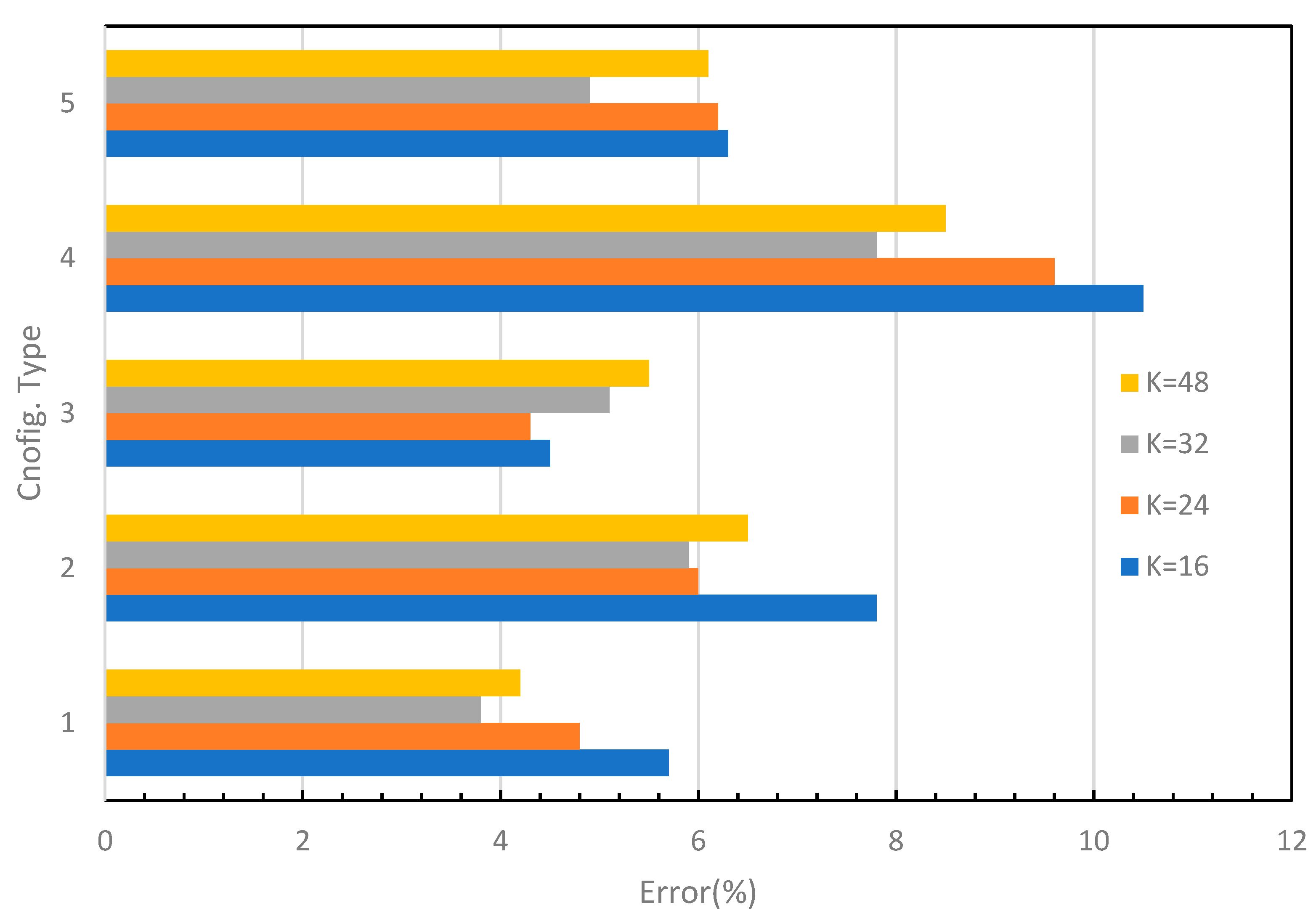
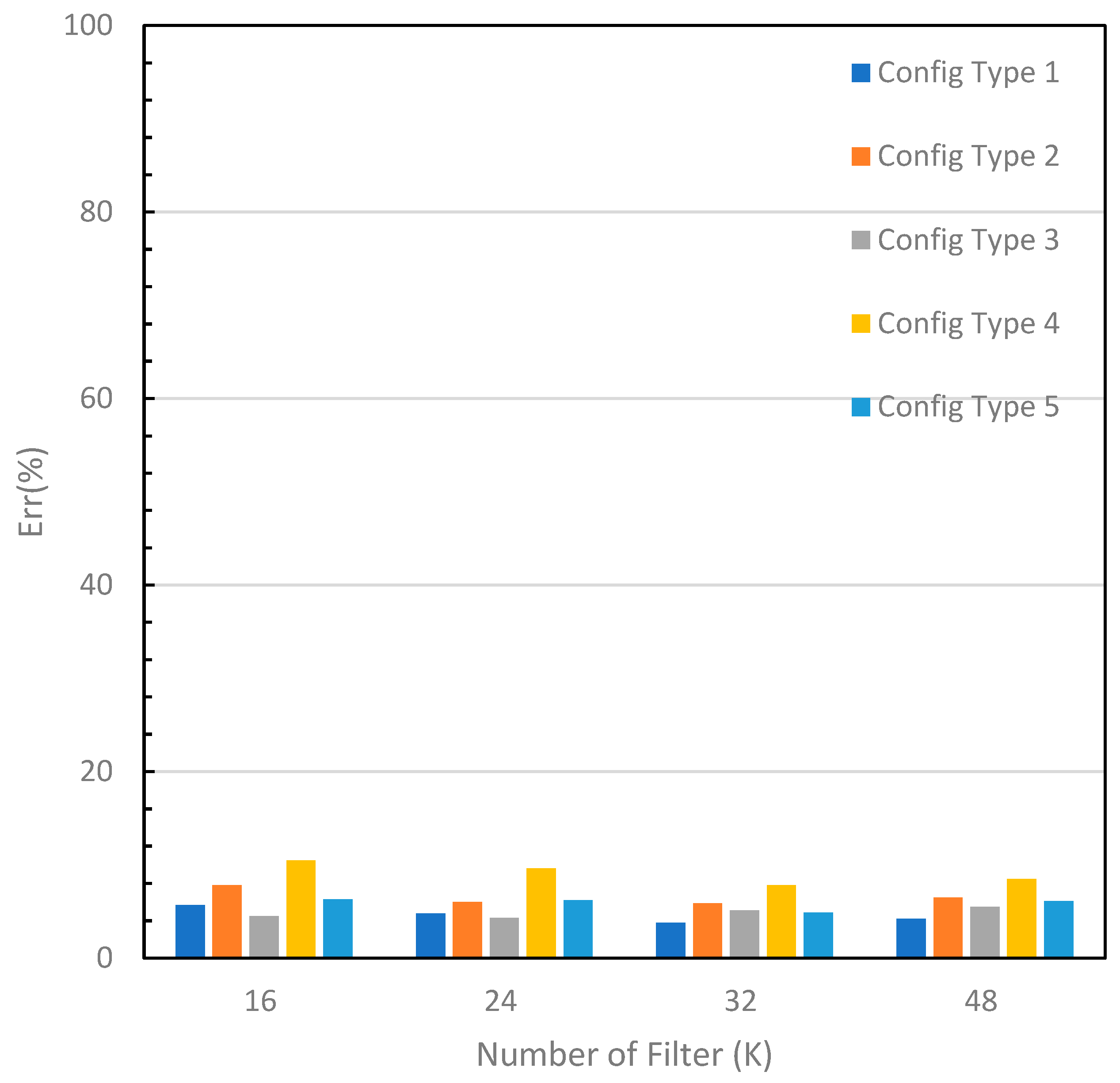
| Architecture | Accuracy | ||
| K | Configuration | training | testing |
| 16 | C1 | 98.6% | 94.3% |
| C2 | 96.3% | 92.2% | |
| C3 | 98.7% | 95.5% | |
| C4 | 93.7% | 89.5% | |
| C5 | 96.6% | 93.7% | |
| 24 | C1 | 99.2% | 95.2% |
| C2 | 98.9% | 94.0% | |
| C3 | 99.0% | 95.7% | |
| C4 | 95.7% | 90.4% | |
| C5 | 98.1% | 93.8% | |
| 32 | C1 | 99.5% | 96.2% |
| C2 | 98.2% | 94.1% | |
| C3 | 98.9% | 94.9% | |
| C4 | 95.2% | 92.2% | |
| C5 | 98.7% | 95.1% | |
| 48 | C1 | 99.1% | 95.8% |
| C2 | 97.7% | 93.5% | |
| C3 | 98.3% | 94.5% | |
| C4 | 96.8% | 91.5% | |
| C5 | 98.2% | 93.9% | |
| class | Type 1 (C1) | Type 2 (C2) |
| O | 93.82% | 92.08% |
| C | 98.32% | 96.16% |
| L | 96.96% | 95.22% |
| Y | 95.71% | 93.03% |
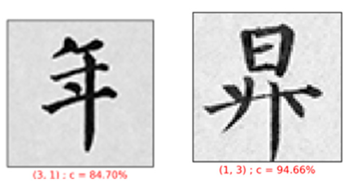
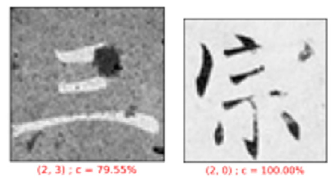
5. Conclusions and future works
- Development of a comprehensive image dataset for Chinese calligraphy (regular script) classification, comprising over 8,000 images, serving as a valuable resource for future scholarly endeavors.
- Pioneering the application of CNN in the classification of personal styles in Chinese calligraphy.
- Achieving elevated performance metrics with the CNN model, evidenced by accuracy rates ranging from 89.5% to 96.2%.
Author Contributions
Data Availability Statement
Conflicts of Interest
References
- Liu, S. (Ed.). (2003). Full Colour Art History of Chinese Calligraphy (1st ed.). Ningxia People's Publishing House. pp. 114-115.
- Huang, Q., & Balsys, R.J. (2009). Applying Fractal and Chaos Theory to Animation in the Chinese Literati Tradition. In Proceedings of the Sixth International Conference on Computer Graphics, Imaging and Visualization, CGIV '09. [CrossRef]
- Fitzgerald, C. P. (1969). The horizon history of China. American Heritage Publishing Co., Inc.
- Wong, E. (1997). The Shambhala Guide to Taoism. Shambhala Publications, Inc.
- Y. LeCun, L. Bottou, Y. Bengio, P. Haffner, Gradient-based learning applied to document recognition, Proc. IEEE 86 (11) (1998) 2278–2324. [CrossRef]
- W. Li, Research on Key Technologies of Chinese Calligraphy Synthesis and Recognition for Chinese Character of Video, Ph.D. Thesis, School of Information Science and Engineering, Xiamen University, Xiamen, China, 2013.
- Y. Lin, Research and Application of Chinese Calligraphic Character Recognition, Ph.D. Thesis, College of Computer Science, Zhejiang University, Hangzhou, China, 2014.
- T. J. Mao, Calligraphy Writing Style Recognition, Ph.D. Thesis, College of Computer Science, Zhejiang University, Hangzhou, China, 2014.
- X. Wang, X. F. Zhang and D. Z. Han, Calligraphy style identification based on visual features, Modern Computer, vol.21, pp.39-46, 2016.
- Y. F. Yan, Calligraphy Style Recognition Based on CNN, Ph.D. Thesis, College of Information and Computer, Taiyuan University of Technology, Taiyuan, China, 2018.
- Cui, W., & Inoue, K. (2021). Chinese calligraphy recognition system based on convolutional neural network. ICIC Express Letters, 15(11), 1187-1195. [CrossRef]
- L. Chen, "Research and Application of Chinese Calligraphy Character Recognition Algorithm Based on Image Analysis," 2021 IEEE International Conference on Advances in Electrical Engineering and Computer Applications (AEECA), Dalian, China, 2021, pp. 405-410. [CrossRef]
- Liu, J., Liu, Y., Wang, P., Xu, R., Ma, W., Zhu, Y., Zhang, B. (2021) Fake Calligraphy Recognition Based on Deep Learning, Lecture Notes in Computer Science (including subseries Lecture Notes in Artificial Intelligence and Lecture Notes in Bioinformatics), 12736 LNCS, pp. 585-596.
- C. Zhai , Z. Chen , J. Li , B. Xu , Chinese image text recognition with BLSTM-CTC: a segmentation-free method, in: 7th Chinese Conference on Pattern Recognition - (CCPR), 2016, pp. 525–536 .
- [15]B. Li, Convolution Neural Network for Traditional Chinese Calligraphy Recognition, CS231N Final Project, http://cs231n.stanford.edu/reports/2016/pdfs/257 Report.pdf, 2016.
- J. Zou, J. Zhang and L. Wang, Handwritten Chinese character recognition by convolutional neural network and similarity ranking, arXiv.org, arXiv: 1908.11550, 2019.
- Y. Wen and J. S. Sig¨uenza, Chinese calligraphy: Character style recognition based on full-page document, Proc. of the 2019 8th International Conference on Computing and Pattern Recognition (ICCPR'19), pp.390-394, 2019. [CrossRef]
- Wang, M., Fu, Q., Wang, X., Wu, Z., & Zhou, M. (2016). Evaluation of Chinese calligraphy by using DBSC vectorization and ICP algorithm. Mathematical Problems in Engineering, 2016, 4845092. [CrossRef]
- Gao, P., Gu, G., Wu, J., & Wei, B. (2017). Chinese calligraphic style representation for recognition. International Journal on Document Analysis and Recognition (IJDAR), 20(1), 59-68. [CrossRef]
- Wang, L., Zhang, J., & Zou, J. (2023). Handwritten Chinese character recognition by convolutional neural network and similarity ranking. In Proceedings of the Conference on Handwritten Chinese Character Recognition (HCCR 2023) (pp. 105-110). Department of Electrical and Computer Engineering, University of Western Ontario.
- D.H. Hubel, T.N. Wiesel, Receptive fields and functional architecture of monkey striate cortex, J. Physiol. (1968) 215–243. [CrossRef]
- K. Fukushima, S. Miyake, Neocognitron: a self-organizing neural network model for a mechanism of visual pattern recognition, in: Competition and Cooperation in Neural Nets, 1982, pp. 267–285.
- Goodfellow, I., Bengio,Y., and Courvile, A. (2016). Deep learning (Vol.). Cambridge, Massachusetts.
- A. Krizhevsky, I. Sutskever, and G. Hinton. Imagenet classification.
- with deep convolutional neural networks. NIPS Conference, pp. 1097–1105. 2012.
- K. Simonyan and A. Zisserman. Very deep convolutional networks for large-scale image recognition.arXiv:1409.1556, 2014. https://arxiv.org/abs/1409.1556.
- Zhou, Bolei, Aditya Khosla, Agata Lapedriza, Antonio Torralba, and Aude Oliva. "Places: An image database for deep scene understanding." arXiv preprint arXiv:1610.02055 (2016).
- K. He, X. Zhang, S. Ren, and J. Sun. Deep residual learning for image recognition. IEEE Conference on Computer Vision and Pattern Recognition, pp. 770–778, 2016.
- Jiuxiang Gu etc. (2018) Pattern Recognition 77, 354-377. Recent advances in convolutional neural networks. [CrossRef]
- LeCun Y., Bengio Y., Hinton G. 2015 Deep Learning. Nature, 521 (7553),436-444. [CrossRef]
- Yangfan Zhou, Xin Wang, Mingchuan Zhang, Junlong Zhu, Ruijuan Zhen, and Qingtao Wu (2015) MPCE: A maximum probability based cross-entropy loss function for neural network classification. IEEE Access, Volume 7, 146331-146341. [CrossRef]
- Toshi Sinha, Ali Haidar, Brijesh Verma, Particle swarm optimization based approach for finding optimal values of convolutional neural network parameters, 2018 IEEE Congress on Evolutionary Computation (CEC), pp.1-6. [CrossRef]
- https://www.tensorflow.org/tutorials/images/classification.
- Justin M. Johnson, and Taghi M. Khoshgoftaar. 2019. Volume 6, 1-54, Journal of Big Data. Survey on deep learning with class imbalance.
- Szilvia Szeghalmy, and Attila Fazekas. Sensors, MDPI (in press).A Comparative Study of the Use of Stratified Cross-Validation and Distribution-balanced Stratified Cross-Validation Imbalanced Learning. [CrossRef]
Disclaimer/Publisher’s Note: The statements, opinions and data contained in all publications are solely those of the individual author(s) and contributor(s) and not of MDPI and/or the editor(s). MDPI and/or the editor(s) disclaim responsibility for any injury to people or property resulting from any ideas, methods, instructions or products referred to in the content. |
© 2023 by the authors. Licensee MDPI, Basel, Switzerland. This article is an open access article distributed under the terms and conditions of the Creative Commons Attribution (CC BY) license (http://creativecommons.org/licenses/by/4.0/).


