Development of a Novel Lightweight Utility Pole Using a New Hybrid Reinforced Composite—Part 2: Numerical Simulation and Design Procedure

Preprint

Article

Development of a Novel Lightweight Utility Pole Using a New Hybrid Reinforced Composite—Part 2: Numerical Simulation and Design Procedure

Altmetrics

Downloads

Views

Comments

A peer-reviewed article of this preprint also exists.

This version is not peer-reviewed

Submitted:

29 November 2023

Posted:

30 November 2023

You are already at the latest version

Alerts

Abstract

The first paper of this two-part series paper discussed the development of a novel lightweight 3D wood dowel-reinforced glass epoxy hybrid composite material (3DdrFRP) and its manufacturing procedures. It also experimentally compared the performance of scaled utility poles made from conventional 2D E-glass epoxy and 3DdrFRP materials. In the second part, we developed robust finite element (FE) models in LS-DYNA, calibrated them based on experimental results, and used them to simulate the performance of equivalent 2D and 3D poles, proving the integrity of the numerical model. Additionally, we developed a simplified analytical calculation method for engi-neers to determine the stiffness of 3D-DrFRP poles accurately and quickly.

Keywords:

Subject: Engineering - Mechanical Engineering

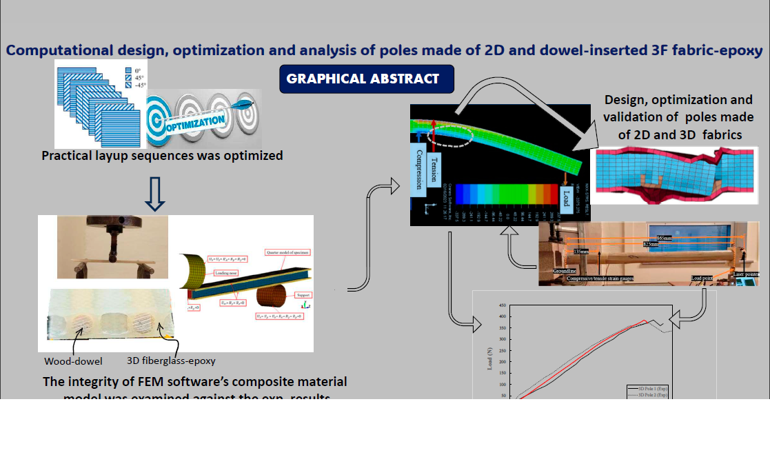
1. Introduction

In the first part of these papers, we provided a detailed history of utility poles and discussed the advantages of fiber-reinforced polymer composites (FRP) poles [1]. Notably, companies like RS Technologies Inc. [2] design modular GFRP poles, offering transportation efficiency and easy replacement of failed modules. In the second part, we designed two poles using the finite element method: a modular 2D cross-ply E-glass epoxy pole and a prismatic pole made of the wood dowel-reinforced 3D E-glass-epoxy hybrid composite. This study emphasizes the importance of FEM for cost-effective and durable laminated composite poles.

2. Design Protocols

Currently, there is no established unified design methodology for FRP poles, but CSA [3] suggests using load factors similar to those used for steel poles. These factors scale up various pole loads. This study employs FEM to design two different poles: a modular 2D cross-ply E-glass epoxy pole and a prismatic pole made of the wood dowel-reinforced 3D E-glass-epoxy hybrid composite, introduced in the first part of these papers. FEM helps consider critical performance and loading conditions [4], cost, and durability factors with minimal testing requirements, particularly the strength in the hoop direction and interlaminar failures. This design approach aligns with modern aircraft structural design involving laminated composites (e.g., Boeing 787 and the Airbus A350 XWB) [5,6].

3. Numerical Simulation Framework

As discussed in the first part of this series [7], 3DdrFML is a complex hybrid material, consisting of a 3D E-glass fabric epoxy with wooden dowels inserted into its channels. Designing a pole using this material requires a sophisticated numerical (finite element (FE)) framework to account for anomalies like local buckling and delamination. The simulation details are presented in the following sections, using the LS-DYNA commercial software, known for its composite material models, contact algorithms, and element birth/death capabilities[8]. Different element types, constituent materials, and contact algorithms to develop a modelling framework for simulating 3DdrFML’s performance.

3.1. Simulation of the behaviour of the flexural 3DdrFML specimens

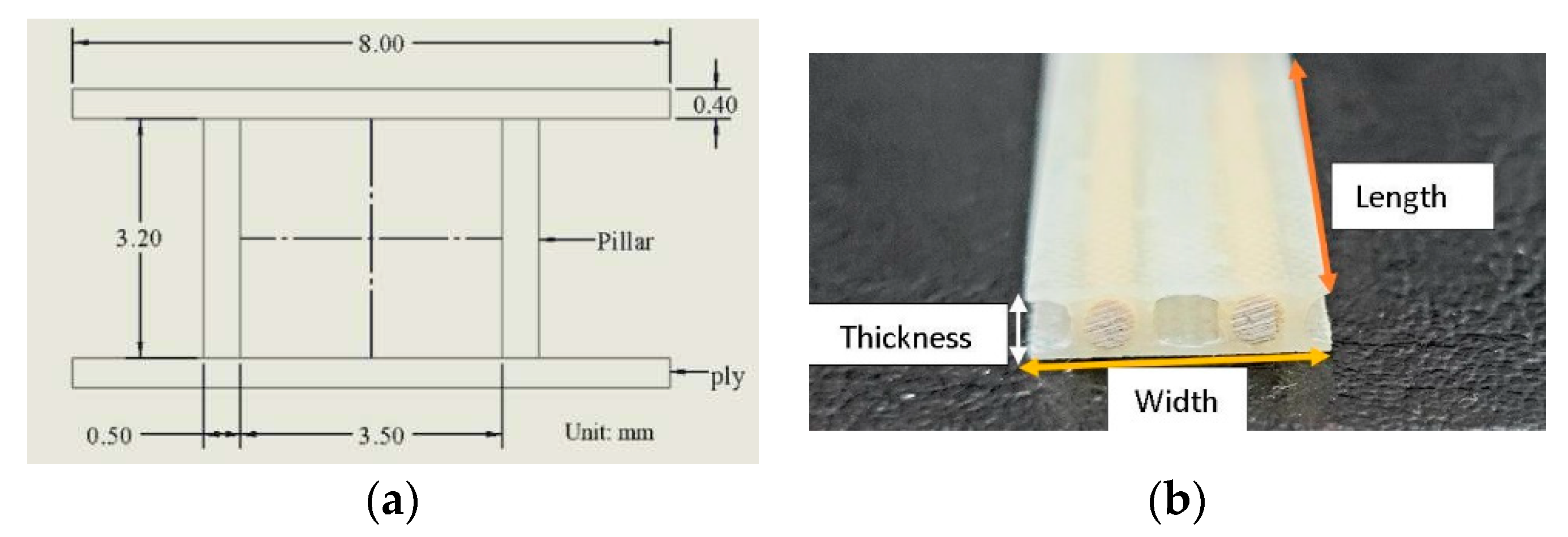
In this study, the behaviour of the 3DdrFML test specimens considered in the first part of the paper was simulated, focusing on various computational algorithms. To assess these, a preliminary finite element model mimicking a flexural test was created, with dimensions of 153(L)x15(W)x4(T) mm (Figure 1).

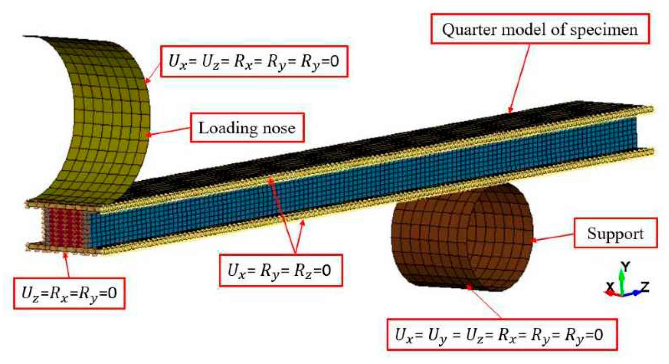
Due to symmetry, only a quarter model was needed (see Figure 2).

The selective reduced-integrated (SRI) Tshell element [9] was incorporated for plies and pillars to prevent shear-locking. The dowels were modelled using solid elements with the SRI formulation, which accounted for poor aspect ratios. Contact interfaces were modelled using the automatic surface-to-surface tie-break contact algorithm, with the option of incorporating the cohesive zone model (CZM) to account for potential delamination or loss of contact between dowels and FRP. The values of the CZM parameters were obtained from reference [10] as presented in Table 1.

The model also considered loading nose-to-specimen and support nose-to-specimen interfaces with frictional coefficients set to 0.3. Additionally, the eroding surface-to-surface algorithm was incorporated to address potential fabric layer ruptures.

The constitutive composite material model (MAT_054) was used for describing 3D fabric epoxy and its pillars, which includes an enhanced damage detection algorithm. The mechanical properties used are shown in Table 1. The dowel’s properties were based on published results [11] and tuned using experimental data, using LS-DYNA’s MAT_143 orthotropic material for wood [8]. The pillar fibers were oriented at 30° with respect to the through-thickness axis of the fabric. The refined material properties used in flexural and compressive models are listed in Table 2.

3.2 Results and Discussions

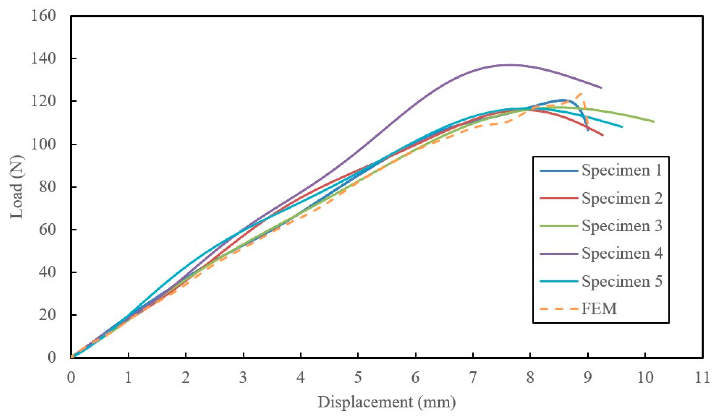
Table 3. Comparison of the average experimental values against the numerically predictedshows the results of numerical simulations of flexural specimen responses, which closely matched experimental results. The error margin of 10.5% can be attributed to slight non-uniform mechanical properties in the complex hybrid configuration and fabrication method. Despite this margin, the numerical results are acceptable, demonstrating the accuracy of our developed numerical framework. See Figure 3 for a comparison of load-displacement responses.

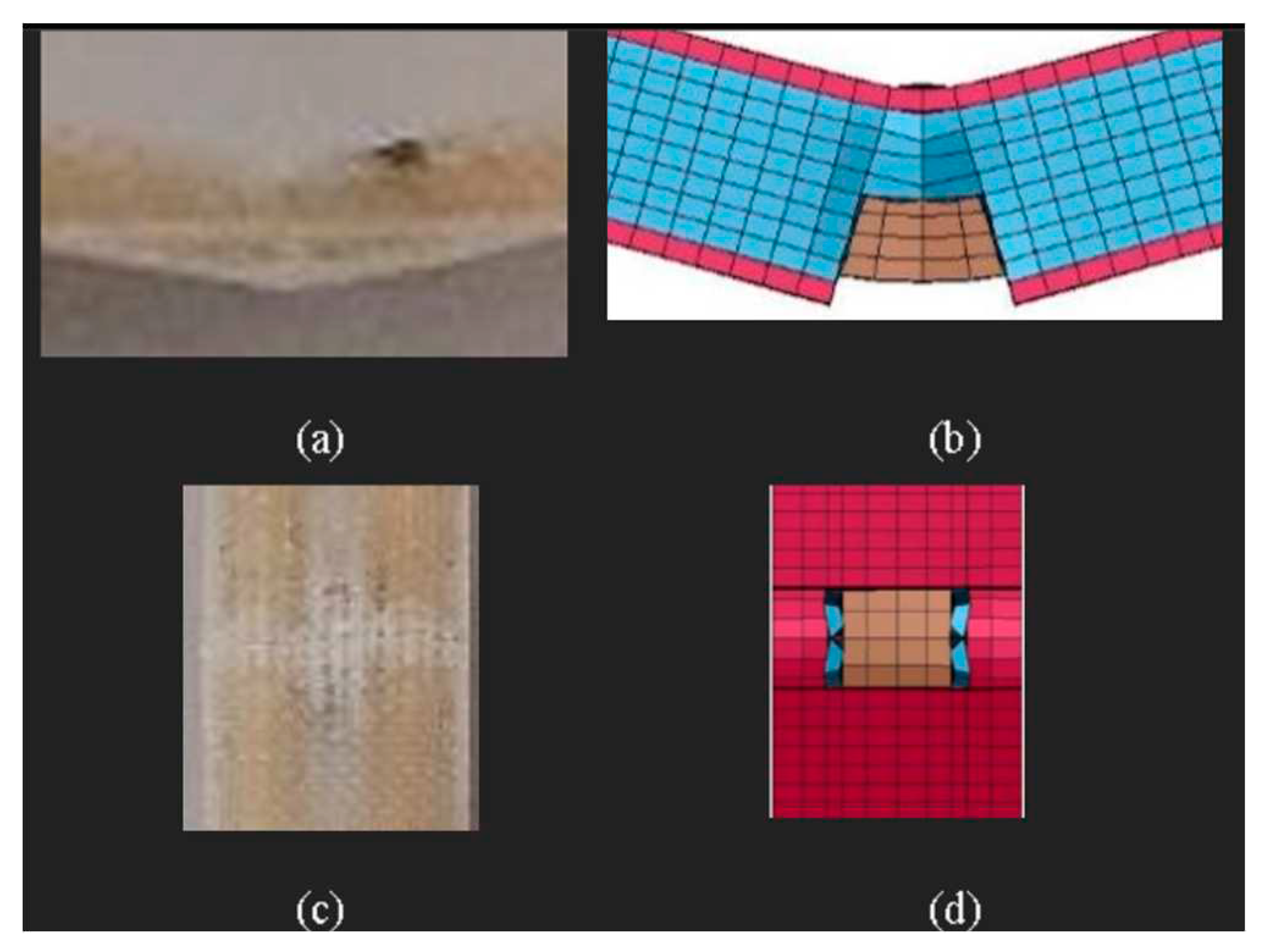
To further validate the model, we compared the damage pattern predicted by the numerical model to the actual specimen response. The FE model successfully simulated ply and pillar failures by deleting highly stressed elements in the damaged region. The most vulnerable region was the ply region on top of the empty channel, which was also captured by the numerical simulation (Figure 4). 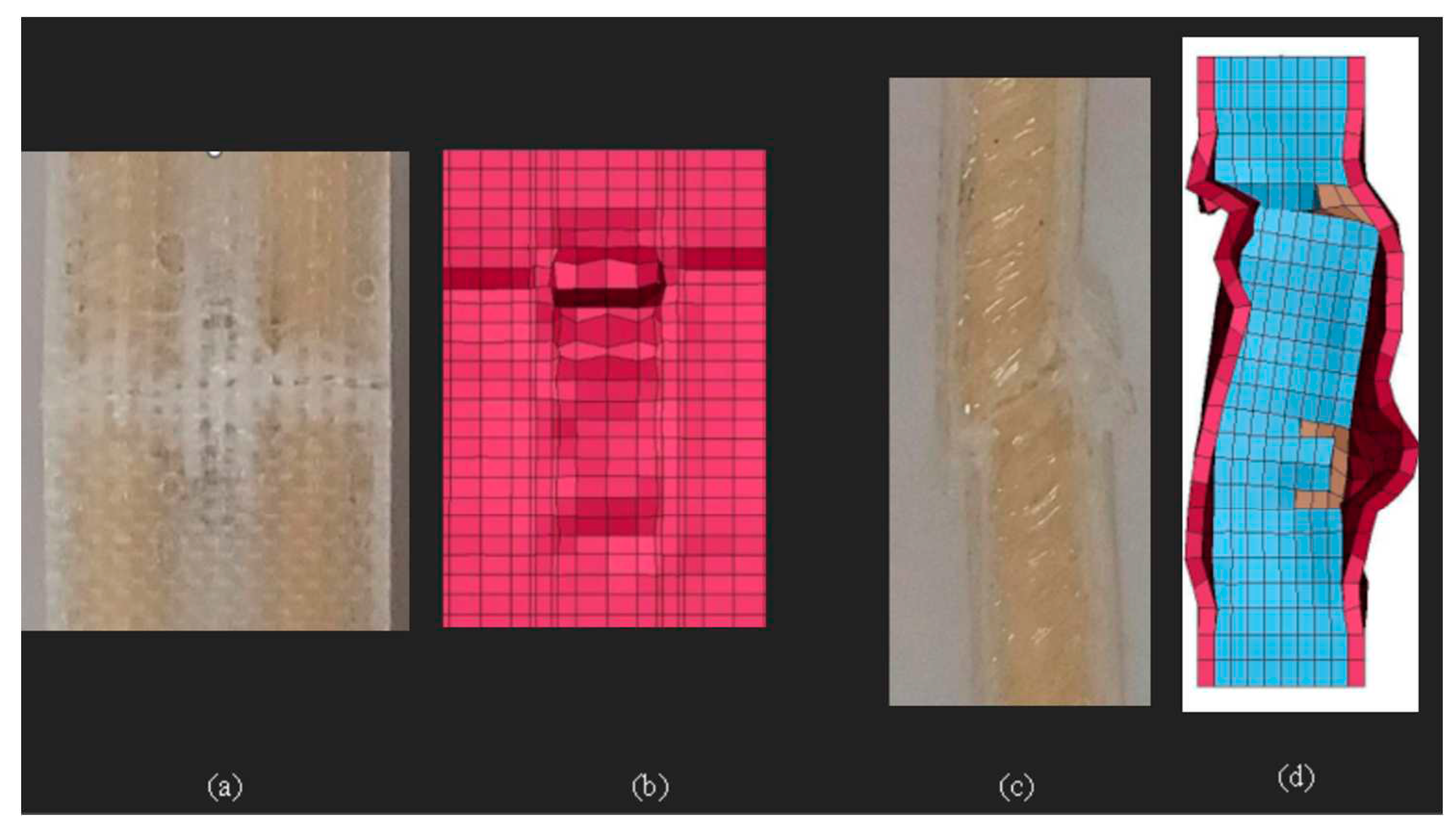The simulated response of compression test specimens, with summarized results in Table 4 and a comparison of experimental and numerical failure modes in Figure 5.

4. Pole Designs

With confidence in the mechanical properties and numerical algorithms established, the design and analysis of two types of scaled-down composite poles: (i) a conventional 2D FRP (like commercially available poles) and (b) the introduced 3D-drFRP material were carried out. While the 2D pole was designed in a modular form due to its advantages, the 3D poles could not take advantage of modularity. Both pole types were designed using 3D solid layered elements for material failure examination, utilizing the Maximum Stress failure criterion for optimal laminate stacking sequence.

4.1. Preliminary Analyzes

4.1.1. Establishment of an effective layup

Prior to designing the 2D and 3D poles, preliminary analyses were conducted to determine effective ply sequencing and optimal element types. Different layups, including combinations of unidirectional and [0/90] cross-ply E-glass fabrics, were examined for potential interlaminar failure. For instance, a 2 m long prismatic pole made of 2D fabric, with its particulars shown in Table 5. Particulars of the test pole to examine the effect of various ply sequences, was analyzed with seven different layup sequences as tabulated in Table 6. The analysis results showed that the [+/0₉/+] laminate, due to its practicality and adequate stiffness, would be the suitable layup for fabrication over [013] layup, which has the highest stiffness, while the [90/011/90] stacking sequence was also investigated to assess interlaminar stresses.

4.1.2. Influence of Element Formulation

The influence of element formulation was explored by comparing the performance of 3D solid elements to Tshell elements. The tip displacement of the pole with [+/0₉/+] layup was analyzed using both element types. The results reported in Table 7 showed that the Tshell element provided good accuracy with significantly lower CPU consumption, improving efficiency by 3,856%. Both elements provided sufficiently accurate results, with small margins of error compared to the analytical solution.

Table 5. Particulars of the test pole to examine the effect of various ply sequences.

Geometric features	Length = 2000 mm	ID = 48 mm	Total thickness=2.6
Boundary conditions	Pole embedment height (mm)	Distance of load from the tip (mm)	Load magnitude (N)
Boundary conditions	200	100	793

4.2. Design of the Modular Pole made of 2D fabric

The design of the 2D modular pole involved two one-meter-long modules due to limitations in the hand layup fabrication process. The pole was designed with a [+/0₉/+] layup and tested against a commercially available pole [2] and other designs from the literature (see Table 8). The modelling considered symmetry, and the Tshell element was used for half of the pole. 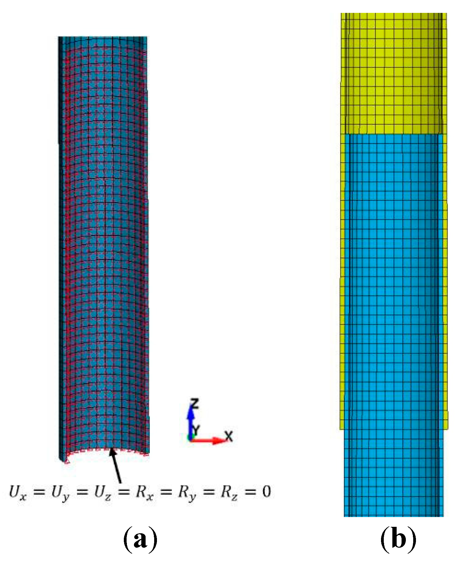The overlap region dimensions were designed according to ASCE’s recommendations [4]. To conserve CPU, nodes within the overlap region were merged with the boundary condition, applied to all the inner surface nodes within 235 mm distance measured from the bottom edge of fully constrained (identified with red triangular symbols in Figure 6(a)). The damage model (MAT_054) was implemented, with mechanical properties provided by Ekşi and Genel [12] as tabulated in Table 9.

Table 6. Numerical failure indices for various laminated designs.

	[+2/05/+2]	[+4/05]	[90/011/90]	[+7]	[013]	[+/09/+]	[+/90/07/90/+]
Longitudinal tension failure	FL	FL	P	FL	P	P	FL
Transverse tension failure	P	P	FL	P	P	P	FL
In-plane shear failure	FL	FL	P	FL	P	P	FL
Through-thickness tension failure	FL	FL	FL	FL	P	P	FL
Through-thickness shear failure	P	P	P	P	P	P	FL
Longitudinal compression failure	FL	FL	P	FL	P	P	FL
Transverse compression failure	P	P	P	P	P	P	P
Through-thickness compression failure	FL	P	FL	P	P	P	FL

Table 7. Comparison of the theoretical maximum tip deflection and bending stress of the pole against numerically predicted values based on element type.

	Solid elements	Tshell elements	Analytical	Solid elements% error	Tshell elements% error
Maximum deflection (mm)	349.3	361.8	352	0.7	2.8
Maximum bending stress (MPa)	133	116	137.3	3.2	15.5
CPU Time (sec)	989	25	-	-	-

Table 8. Comparison of the proposed pole design with the commercial pole and scaled poles from other studies.

	Proposed design (assembled)	RS Technologies	Pole of Ref. [13]	Pole of Ref. [14]
Slenderness ratio	165.7	219.2	127.7	83.0
𝐷𝑎𝑣𝑔/t	20.7	27.5	19.4	65.5

Table 9. Mechanical properties used in the FE model of the 2D modular pole.

Fabric Type	𝝆 (𝒈/𝒎𝒎𝟑)	𝑬𝟏𝟏 (M𝑷𝒂)	𝑬𝟐𝟐 (M𝑷𝒂)	𝝊𝟐𝟏	𝑮𝟏𝟐 (M𝑷𝒂)	𝑮𝟐𝟑 (M𝑷𝒂)	𝑮𝟑𝟏 (M𝑷𝒂)
Fabric Type	0.00175	15,560	6,749	0.11	3,310.8	2,595.8	3,310.8
UD	𝑿𝑪 (M𝑷𝒂)	𝑿𝑻 (M𝑷𝒂)	𝒀𝑪 (M𝑷𝒂)	𝒀𝑻 (M𝑷𝒂)	𝑺𝟏𝟐 (M𝑷𝒂)
	343.3	572.2	80.1	78	30.9
	𝝆 (𝒈/𝒎𝒎𝟑)	𝑬𝟏𝟏 (M𝑷𝒂)	𝑬𝟐𝟐 (M𝑷𝒂)	𝝊𝟐𝟏	𝑮𝟏𝟐 (M𝑷𝒂)	𝑮𝟐𝟑 (M𝑷𝒂)	𝑮𝟑𝟏 (M𝑷𝒂)
Biaxial [+]	0.00175	9,336	4,049.4	0.11	1,986.4	1,557.5	1,655.4
	𝑿𝑪 (M𝑷𝒂)	𝑿𝑻 (M𝑷𝒂)	𝒀𝑪 (M𝑷𝒂)	𝒀𝑻 (M𝑷𝒂)	𝑺𝟏𝟐 (M𝑷𝒂)
	223.1	343.3	48.1	46.8	18.5

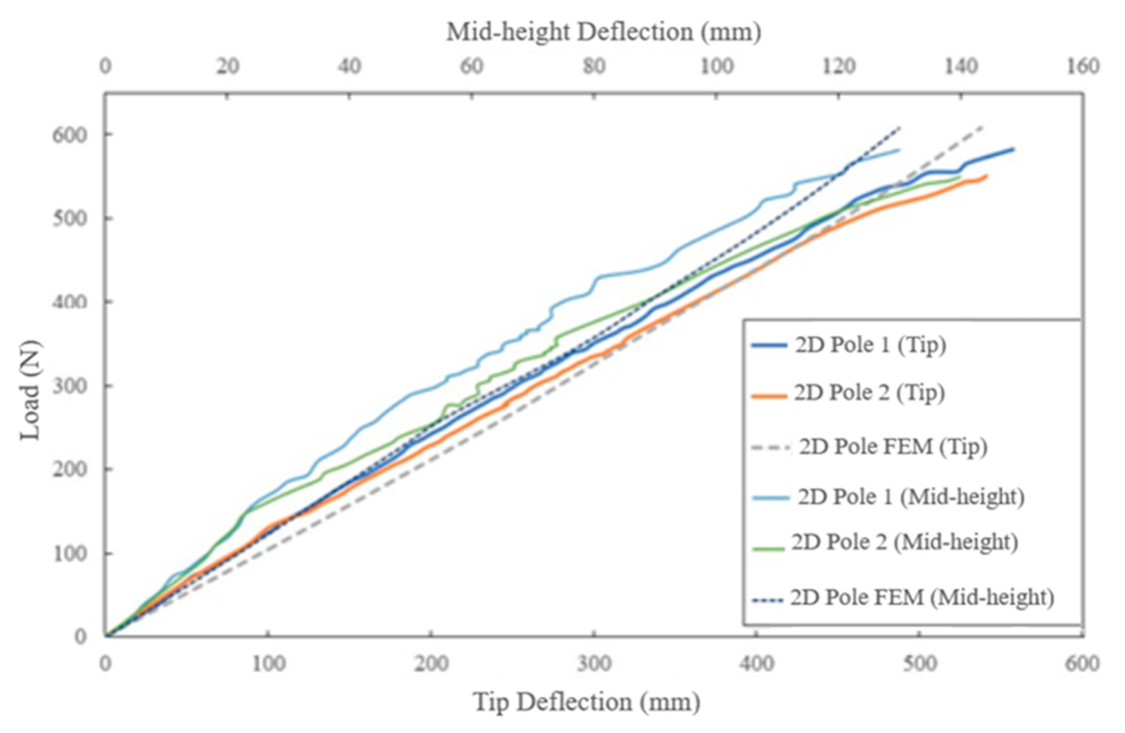
The comparison of the numerical simulation and experimental load-deflection results showed good agreement (see Figure 8), with numerical results being slightly stiffer due to the nature of FEM. The maximum numerical strain reached -0.018 mm/mm at approximately 540 mm deflection, compared to the experimental strain of -0.015 mm/mm at the same deflection. The tensile experimental strain-deflection curves were consistent, and the numerically predicted strains were slightly higher up to a tip deflection of 190 mm when inelastic deformation occurred. The maximum compressive and tensile strains were comparable for both experimental and numerical values.

Figure 7. Comparison of the experimental and numerical load-deflection curves of the 2D poles at the tip and mid-height.

4.3. Scaled pole design

As stated, previously, one of the novel aspects of this work is the incorporation of 3D fabric in developing long-lasting poles, which has not been attempted before. Another novelty is the addition of wooden dowels to reinforce the fabric, enhancing its stiffness, and enabling the use of 3D fabric in cylindrical structural members. Before designing the 3D pole, three-point bending tests were conducted on curved specimens extracted from a 3DdrFRP cylinder. The results in Figure 7 from the previous paper show that dowel reinforcement improved the FRP’s stiffness and strength by approximately 300% and 500%, respectively.

Due to the complex configuration of 3DdrFRP, fabricating a tapered pole would be challenging. The tapered shape would result in a differing number of channels on the top and bottom portions, requiring partial cutting of the dowels along the pole’s length. This impracticality led to the use of a prismatic pole design as a compromise. The pole had specific dimensions with a slenderness ratio close to that of 2D tapered poles, as discussed in the first paper. The pole’s restraint and loading conditions are depicted in Figure 9.

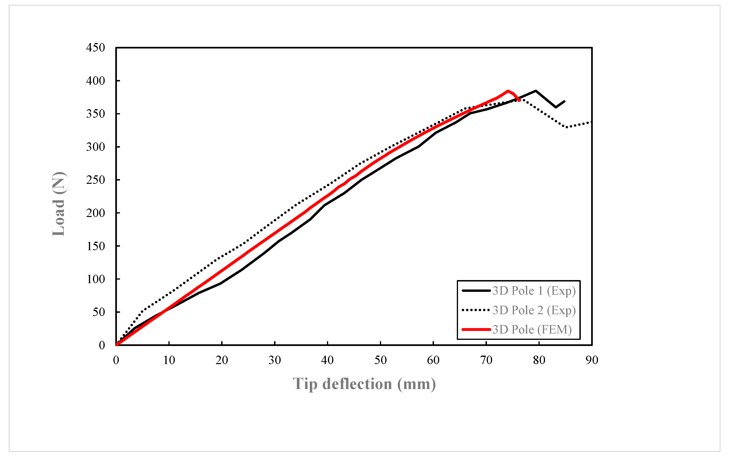
The designed pole was subjected to the same load as the two 3D poles in the experimental investigation. A comparison of the experimental and numerical load-tip deflection curves is shown in Figure 10. The predicted response closely matched the experimental results up to the poles’ failure loads. The FE model’s prediction estimated the pole’s failure load at a slightly lower deflection and a failure load magnitude between the two experimental poles.

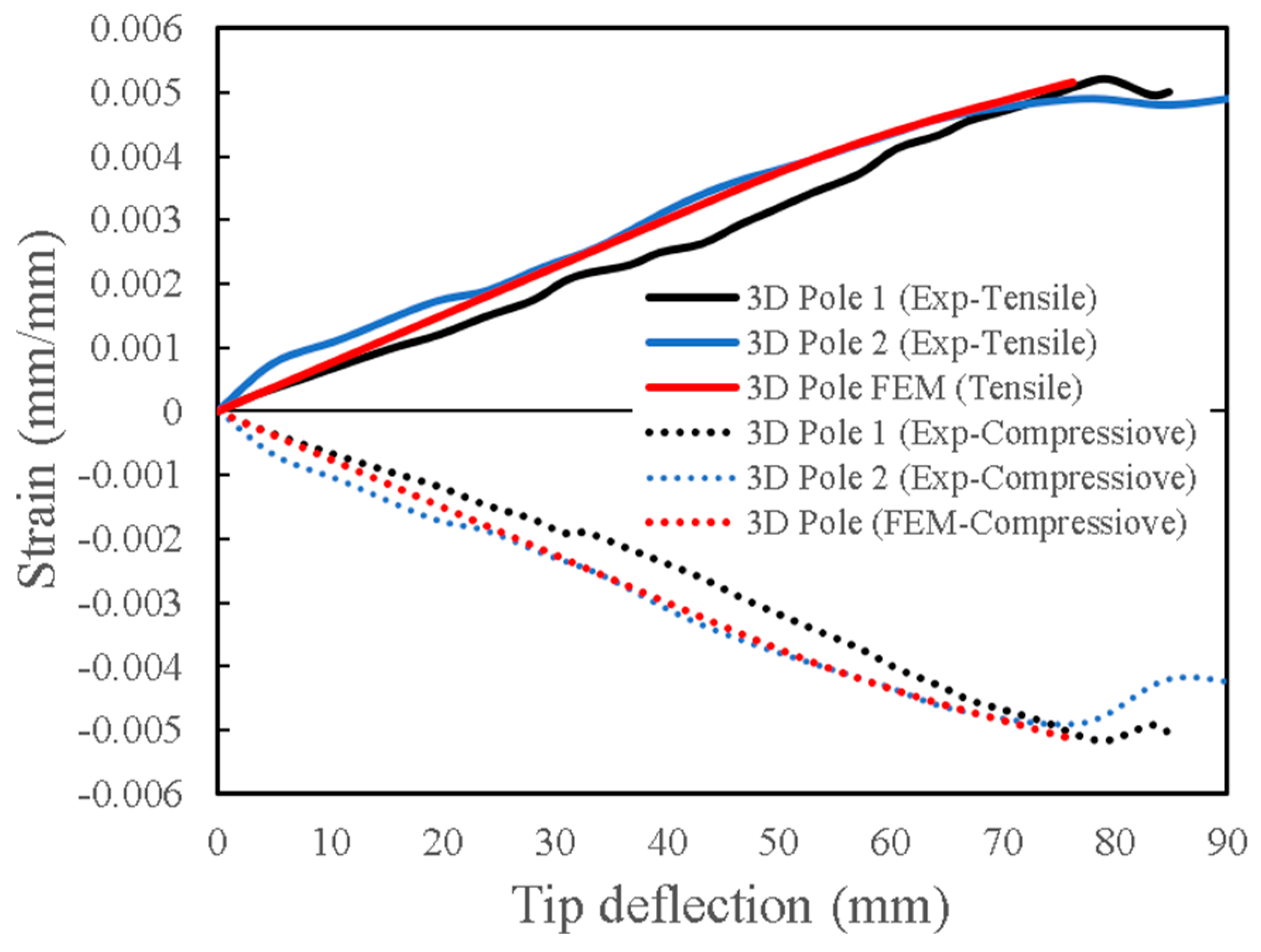
Figure 10 shows that Pole 2 endured significant load after reaching its ultimate strength, gradually decreasing to 262 N before fully fracturing at 220mm deflection. This was accompanied by ply failure above the groundline along an empty channel on the compression side, followed by compression failure observed at the groundline after the fracture. Figure 11 illustrates the comparison of numerically predicted tensile strain values with experimental results, showing close agreement. The ultimate experimental and FE strains and their corresponding deflections are nearly identical to those observed on the compression side of the poles.

Table 10. Comparison of the averaged elastic modulus of the actual and numerically designed poles.

Moment of inertia, I (𝑚𝑚4)		𝐸𝑥 (MPa)	Stiffness (N·mm2)	% Error in 𝐸𝑥
Experiment	115,149.5	9,726.5	1.12E+9	0.89
FEM	115,149.5	9,639.6	1.11E+9	0.89

5. Comparison of the Performance of 2D and 3D poles

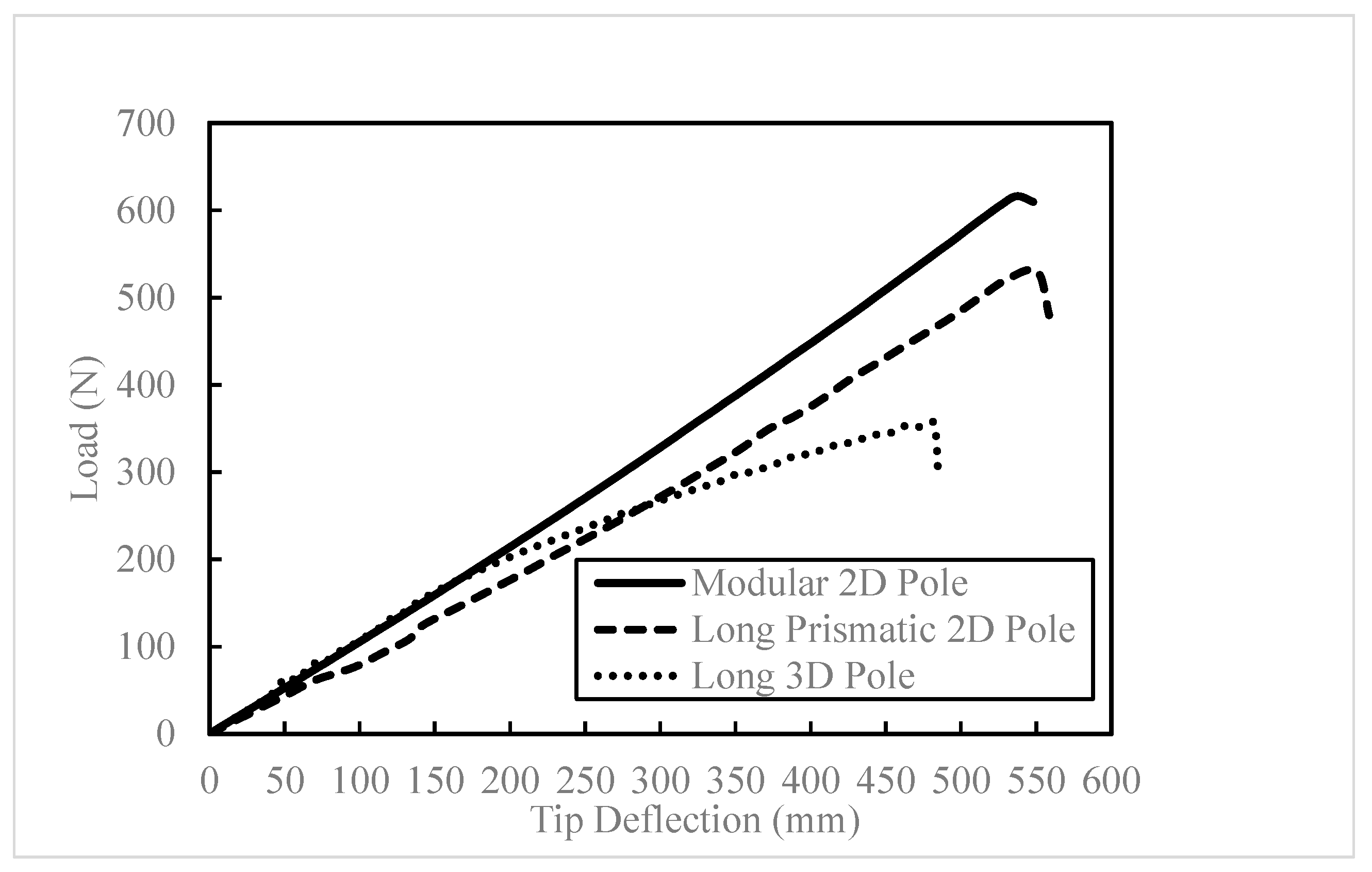
The performances of the two types of poles are compared by normalizing their ultimate strength to their masses. Since the tested 3D poles were shorter and prismatic and the 2D poles were longer and non-prismatic, they could not be compared directly. Therefore, the response of a 3D pole with the same length as the 2D pole is simulated. The outside diameter of this 3D pole is the average of the outside top and bottom diameters of the 2D pole. Additionally, for more consistency, an equivalent prismatic 2D pole is also considered to investigate the effect of the modular design of the 2D pole in comparison to the monolithic pole. The length and outside diameter of these prismatic 2D and 3D poles are the same as the average length and diameter of the modular 2D poles (i.e., 1735 mm and 48 mm, respectively). The results of the analyses are reported in Table 12 and shown in Figure 12.

Table 11. Summary of the fundamental physical parameters of the FE model and the results.

Pole Type	Volume (mm3)	Mass (g)	Stiffness (N·mm2)	Ultimate Load Capacity (N)	Normalized Ultimate Load Capacity (N/kg)
2D Pole	68,6711	760.5	1.02E+09	616.0	0.81
2D Prismatic Pole	57,2920	634.5	9.02E+08	530.0	0.84
Long prismatic 3D Pole	66,9842	729.2	1.06E+09	355.8	0.49

The modular 2D and the longer 3D poles exhibit similar initial stiffness, while the prismatic 2D pole’s stiffness is slightly lower. Surprisingly, the 3D pole’s ultimate strength is noticeably lower than both 2D poles. The 3D pole starts to show damage at a load of 195 N, with a tip deflection of 190 mm, whereas the 2D poles show no damage until reaching their ultimate strength. It should be noted that the 2D poles consist of more fabric layers than the 3D poles.

The unsupported segments of the 3D pole, specifically those over the empty channels, make it more prone to premature failure under a flexure load compared to the segments supported by wood dowels and pillars. The addition of more layers of 2D-FRP or dowel reinforcement in every channel of the 3D fabric could significantly improve its performance.

6. A Simple Equation for Establishing the Stiffness of 3D Poles.

With consideration of Figure 1(a), a simple equation for estimating the stiffness of 3D poles is developed below, by which the extensional elastic modulus of the complex hybrid composite in the principal material direction is established.

E_{3 D, x} \approx E_{3 D, 1} (exact) = \frac{2 A_{Ply} E_{Ply} + A_{Pillar} E_{Pillar} + A_{Dowel} E_{Dowel}}{2 A_{Ply} + 2 A_{Pillar} + A_{Dowel}}

(1)

where 𝐴𝑃𝑙𝑦, 𝐴𝑃𝑖𝑙𝑙𝑎𝑟 and 𝐴𝐷𝑜𝑤𝑒𝑙 are the total cross-sectional areas of the ply, pillar, dowel and empty channels, respectively; 𝐸𝑃𝑙𝑦, 𝐸𝑃𝑖𝑙𝑙𝑎𝑟 and 𝐸𝐷𝑜𝑤𝑒𝑙 are the elastic modulus of the plies, pillars and dowels in the principal material direction 1, respectively.

This equation can be modified and used with the exact net cross-section area or the gross cross-section area, simplifying the calculation process, as follows:

E_{3 D, x} \approx E_{3 D, 1} (approx) = \frac{2 A_{P l y} E_{P l y} + A_{Pillar} E_{Pillar} + A_{Dowel} E_{Dowel} + A_{air} E_{air}}{2 A_{Ply} + 2 A_{Pillar} + A_{Dowel} + A_{air}}

(2)

where and 𝐸_𝐴𝑖𝑟 is the elastic modulus of the air in the empty channels (equal to zero) and 𝐴_𝐴𝑖𝑟 is the total cross-section area of the empty channels. Multiplication of this value of

E_{3 D, x}

with the gross cross-section area would yield exactly the same extensional stiffness as obtained by the use of the exact net cross-section area. The results from the equations are reported in the following table.

Table 12. Comparison of experimental Young’s modulus and those predicted by the established equations.

Method	Extensional elastic modulus (MPa)	Stiffness (N·mm2)	% Error in Stiffness
Experimental value (Compression Test)	8,963.5	152,208
Equation (1)	8,686.0	152,154	0.03
Equation (2)	5,296.0	152,154

Equation (2), can be further simplified for the 4 mm nominal thick 3D fabric used in this study, considering that parameters related to the 3DFRP are constant and the only variable would be the dowel’s elastic modulus as an unknown. Therefore, the following simplified equation could be used instead of the more elaborate version, Equation 1.

𝐸_3𝐷,𝑥 = 3562.2 + 0.45𝐸_{𝑑𝑜𝑤𝑒𝑙}

(3)

It is important to note that this equation is specific to the configuration considered in this study and can be adapted for different fabric thicknesses or pole cross-sections.

7. Summary and Conclusions

The authors previously introduced a novel, lightweight, and stiff utility pole constructed from an innovative 3D fiberglass fabric-epoxy composite material (3DdrFRP) reinforced with wooden dowels. This paper delves into the intricate numerical modelling techniques developed for optimizing the design of such advanced 3D hybrid composite poles. The resulting nonlinear models exhibited a high degree of reliability and accuracy in predicting pole responses, including localized failure modes.

Additionally, this research involved a comparison between LS-DYNA’s 3D solid layered element and its 2D thick-shell (Tshell) counterpart to evaluate prediction accuracy and computational resource utilization. The findings indicated that Tshell yielded results with acceptable accuracy while drastically improving CPU efficiency, reducing consumption by 3,856%.

The numerical analysis further revealed a substantial enhancement in composite stiffness and strength (approximately 300% and 500%, respectively) with the incorporation of dowels into the 3D-FRP composite. The ongoing use of the developed numerical model aims to conduct a parametric study, seeking to optimize the performance of 3D poles and address localized fabric failures effectively.

References

Morrell, J.J. Wood Pole Maintenance Manual. Corvallis, OR: Forest Research Laboratory. Oregon State University, 2012. [Google Scholar]
R S Technologies Inc. RS Poles 2023. Available online: https://www.rspoles.com/.
CSA. Overhead systems, C22.3 No. 1-15 2015.
Recommended Practice for Fiber-Reinforced Polymer Products for Overhead Utility Line Structures, 2nd ed.; Galen, F. (Ed.) American Society of Civil Engineers (ASCE), 2019. [Google Scholar]
Nath, A.; Anand, R.; Desai, J.; Sultan, M.T.H.; Raj, S.A. Modelling and Finite Element Analysis of an Aircraft Wing using Composite Laminates. IOP Conf. Ser. Mater. Sci. Eng. 2021. [Google Scholar] [CrossRef]
Siefert, A.; Henkel, F.O. Nonlinear analysis of commercial aircraft impact on a reactor building—Comparison between integral and decoupled crash simulation. Nucl. Eng. Des. 2014, 269, 130–135. [Google Scholar] [CrossRef]
Wu, J.; Taheri, F. Development of a Novel Lightweight Utility Pole using a New Hybrid Reinforced Composite – Part 1: Fabrication & Experimental Investigation. J. Compos. Sci. 2023. [Google Scholar]
LS-DYNA Keyword User’s Manual, Livermore Software Technology, 13th ed.; 2021; vol. II.
LS-DYNA Keyword User’s Manual, Livermore Software Technology, 13th ed.; 2021; vol. I.
Mohamed, M.; Taheri, F. Fracture response of double cantilever beam subject to thermal fatigue. J. Strain Anal. Eng. Des. 2018, 53, 504–516. [Google Scholar] [CrossRef]
Ross, R. Wood Handbook: Wood as an Engineering Material; Forest Service U.S. Department of Agriculture, 2021. [Google Scholar]
Ekşi, S.; Genel, K. Comparison of Mechanical Properties of Unidirectional and Woven Carbon, Glass and Aramid Fiber Reinforced Epoxy Composites. Acta Phys Pol A 2017, 132. [Google Scholar] [CrossRef]
Altanopoulos, T.I.; Raftoyiannis, I.G.; Polyzois, D. Finite element method for the static behavior of tapered poles made of glass fiber reinforced polymer. Mech. Adv. Mater. Struct. 2021, 28, 2141–50. [Google Scholar] [CrossRef]
Ibrahim, S.M. Performance Evaluation of Fiber-Reinforced Polymer Poles For Transmission Lines; Doctor of Philosophy. Manitoba, n.d.

Figure 1. (a) The dimensions of the 3D E-glass epoxy unit cell used in all numerical models ;(b) A view of the actual flexural specimen.

Figure 2. The quarter symmetry model of the flexural test specimens and the imposed boundary conditions.

Figure 3. Comparison of the load-displacement responses of the flexural specimens and the numerically predicted results.

Figure 4. Comparison of the post-failure damage on the actual specimen and the numerically predicted.

Figure 5. Compression of the experimental and numerically predicted compressive failure modes of a 3DdrFRP specimen under compressive loading (a) experimental front. (b) numerical front view (c) experimental side view (d) numerical side view

Figure 6. (a)Illustration of boundary conditions accounting for the fixture, (b) mesh of the overlap region of the tapered poles.

Figure 9. (a) the fully restrained nodes on the inner surface of the pole, (b) the load ring attached to the pole using contact algorithm.

Figure 10. Comparison of the experimental and numerically and numerically predicted load-deflection curves.

Figure 11. Comparison of experimental and FE strain-tip deflection curves for 3D poles.

Figure 12. Comparison of the 2D and 3D poles.

Table 1. Summary of the epoxy-related parameters required by the CZM contact algorithm.

Normal failure stress (MPa)	Shear failure stress (MPa)	Mode I energy release rate (KJ⁄m2)	Mode II energy release rate (KJ⁄m2)	Penalty stiffness (N/mm3)
59	23	1	1.5	3500

Table 1. Refined material properties used in flexural and compressive models.

Upper and lower plies	𝝆	𝑬𝟏𝟏	𝑬𝟐𝟐	𝝊𝟐𝟏	𝑮𝟏𝟐	𝑮𝟐𝟑	𝑮𝟑𝟏
	(𝒈/𝒎𝒎3)	(M𝑷𝒂)	(M𝑷𝒂))		(M𝑷𝒂)	(M𝑷𝒂)	(M𝑷𝒂)
	0.00175	9000	9000	0.05	1000	1000	1000
	𝑿𝑪 (M𝑷𝒂)	𝑿𝑻 (M𝑷𝒂)	𝒀𝑪 (M𝑷𝒂)	𝒀𝑻 (M𝑷𝒂)	𝑺𝟏𝟐 (M𝑷𝒂)	𝜀𝑇1	𝜀𝐶1
	153	179	153	179	30	0.08	-0.04
Pillars	𝝆	𝑬𝟏𝟏	𝑬𝟐𝟐	𝝊𝟐𝟏	𝑮𝟏𝟐	𝑮𝟐𝟑	𝑮𝟑𝟏
	(𝒈/𝒎𝒎𝟑)	(M𝑷𝒂)	(M𝑷𝒂)		(M𝑷𝒂)	(M𝑷𝒂)	(M𝑷𝒂)
	0.00175	3000	1000	0.05	1000	1000	1000
	𝑿𝑪 (M𝑷𝒂)	𝑿𝑻 (M𝑷𝒂)	𝒀𝑪 (M𝑷𝒂)	𝒀𝑻 (M𝑷𝒂)	𝑺𝟏𝟐 (M𝑷𝒂)	𝜀𝑇1	𝜀𝐶1
	80	80	80	80	30	0.054	-0.054
Dowels	𝝆	𝑬𝑳	𝑬𝑻	𝑮𝑳𝑻	𝑮𝑳𝑹	𝝊𝟏𝟐	𝑿𝑪
	(𝒈/𝒎𝒎𝟑)	(M𝑷𝒂)	(M𝑷𝒂)	(M𝑷𝒂)	(M𝑷𝒂)		(M𝑷𝒂)
	0.0006	11330	974.38	1099.01	1665.51	23671	51.1
	𝑿𝑻	𝒀𝑪	𝒀𝑪	𝑺𝟏𝟐
	(M𝑷𝒂)	(M𝑷𝒂)	(M𝑷𝒂)	(M𝑷𝒂)
	51.1	6.5	8	13.2

Table 3. Comparison of the average experimental values against the numerically predicted.

	Max Load (N)	Max. Disp. (mm)	𝐸𝑓 (MPa)	Flexural Rigidity (N·mm2)	% Error
Exp	134.0	8.6	10,267.1	679,683.3
				608,273.1	10.5
FEM	128.0	8.9	9188.42	608,273.1

Table 4. Comparison of the average experimental values and the numerically predicted values.

	Elastic modulus, 𝐸𝑐 (MPa)	Ultimate Load (N)	Ultimate Strength (MPa)	Ultimate Strain (mm/mm)	% Error in Elastic modulus
Exp	8,963.5	2,747.0	69.5	0.015	9.9
FEM	8080.0	2,556.0	61.4	0.017

Disclaimer/Publisher’s Note: The statements, opinions and data contained in all publications are solely those of the individual author(s) and contributor(s) and not of MDPI and/or the editor(s). MDPI and/or the editor(s) disclaim responsibility for any injury to people or property resulting from any ideas, methods, instructions or products referred to in the content.

© 2023 by the authors. Licensee MDPI, Basel, Switzerland. This article is an open access article distributed under the terms and conditions of the Creative Commons Attribution (CC BY) license (http://creativecommons.org/licenses/by/4.0/).

Copyright: This open access article is published under a Creative Commons CC BY 4.0 license, which permit the free download, distribution, and reuse, provided that the author and preprint are cited in any reuse.

MDPI Initiatives

Important Links

Choose an area of interest and we will send you notifications of new preprints at your preferred frequency.

Disclaimer

Development of a Novel Lightweight Utility Pole Using a New Hybrid Reinforced Composite—Part 2: Numerical Simulation and Design Procedure

Abstract

1. Introduction

2. Design Protocols

3. Numerical Simulation Framework

3.1. Simulation of the behaviour of the flexural 3DdrFML specimens

3.2 Results and Discussions

4. Pole Designs

4.1. Preliminary Analyzes

4.1.1. Establishment of an effective layup

4.1.2. Influence of Element Formulation

4.2. Design of the Modular Pole made of 2D fabric

4.3. Scaled pole design

5. Comparison of the Performance of 2D and 3D poles

6. A Simple Equation for Establishing the Stiffness of 3D Poles.

7. Summary and Conclusions

References

MDPI Initiatives

Important Links

Subscribe