3.2. Dynamic resistance signal characteristics
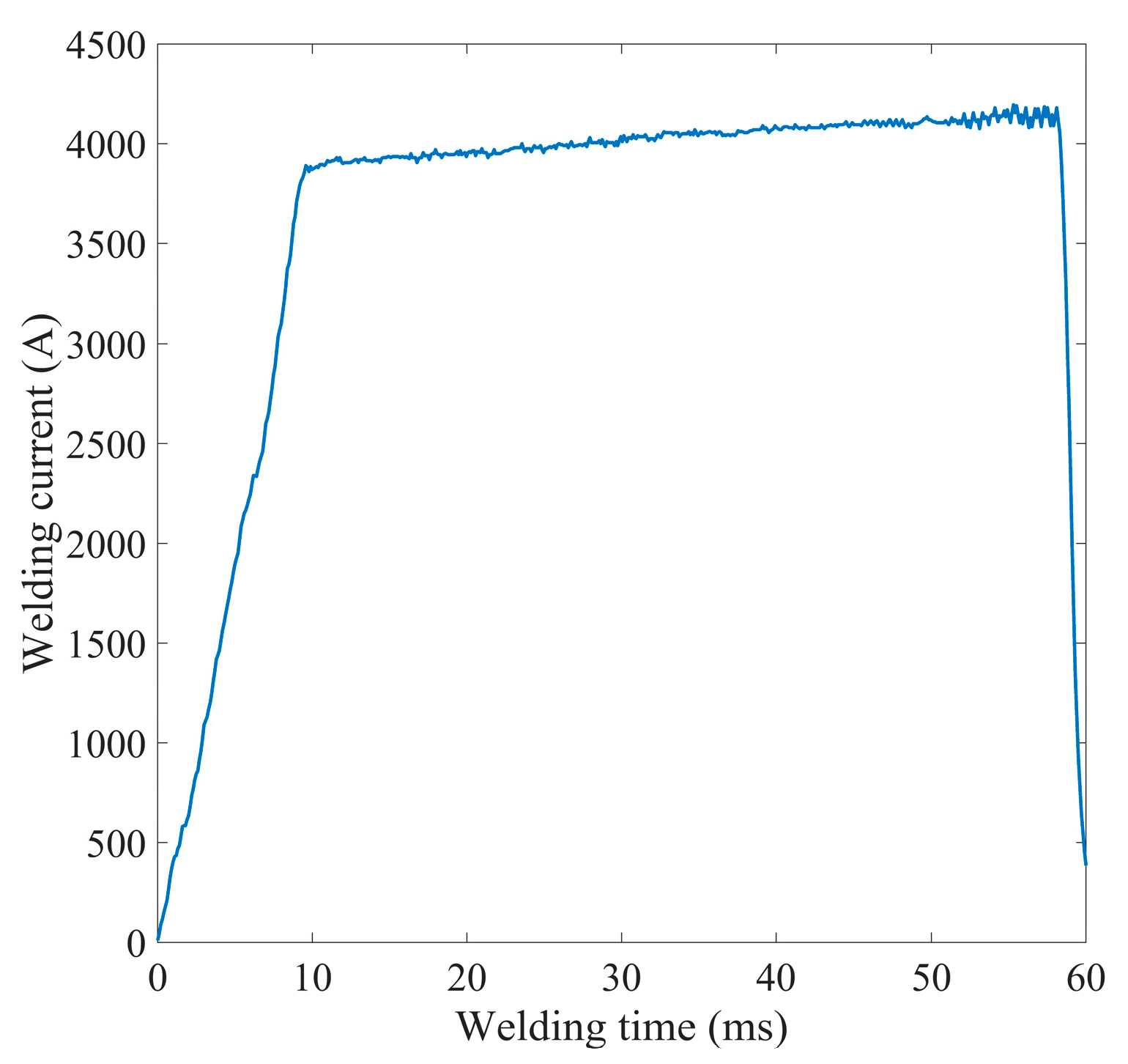
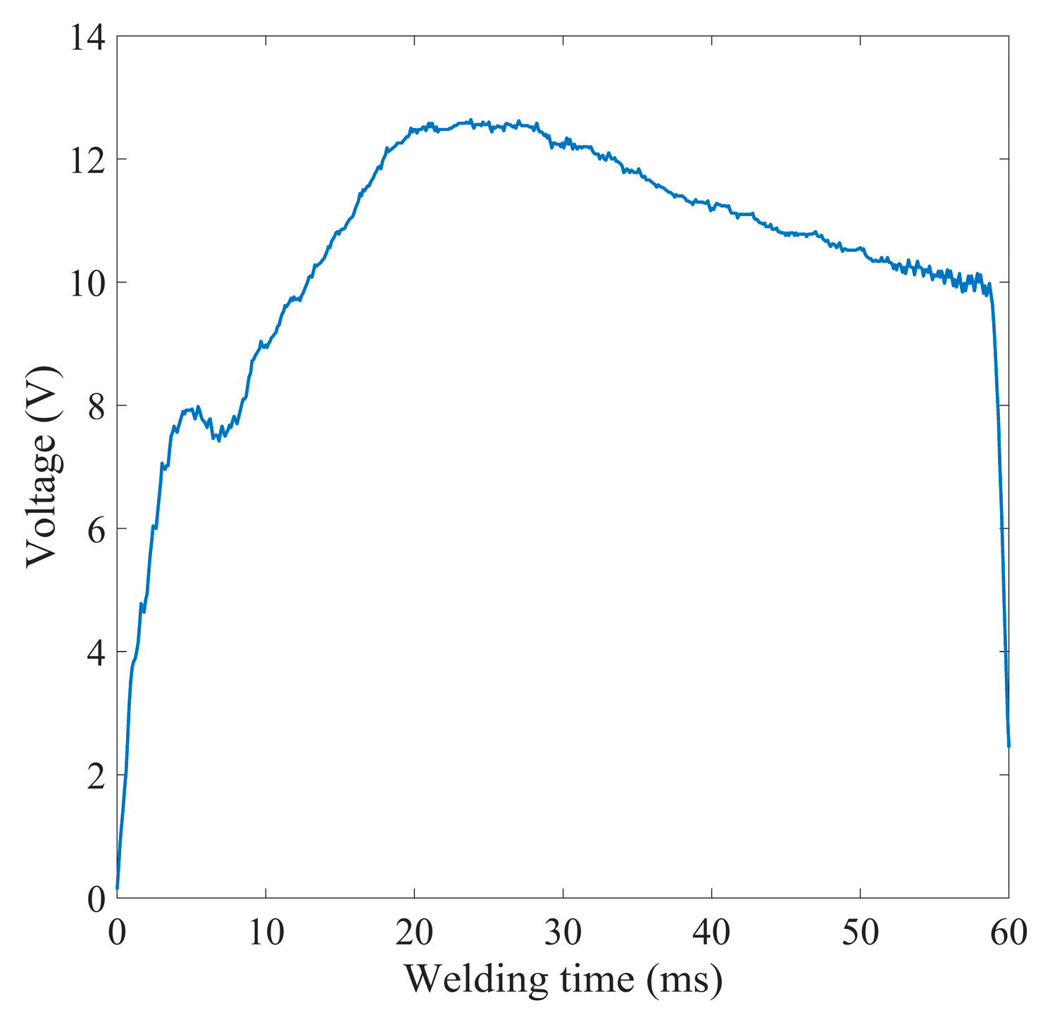
Figure 8 and
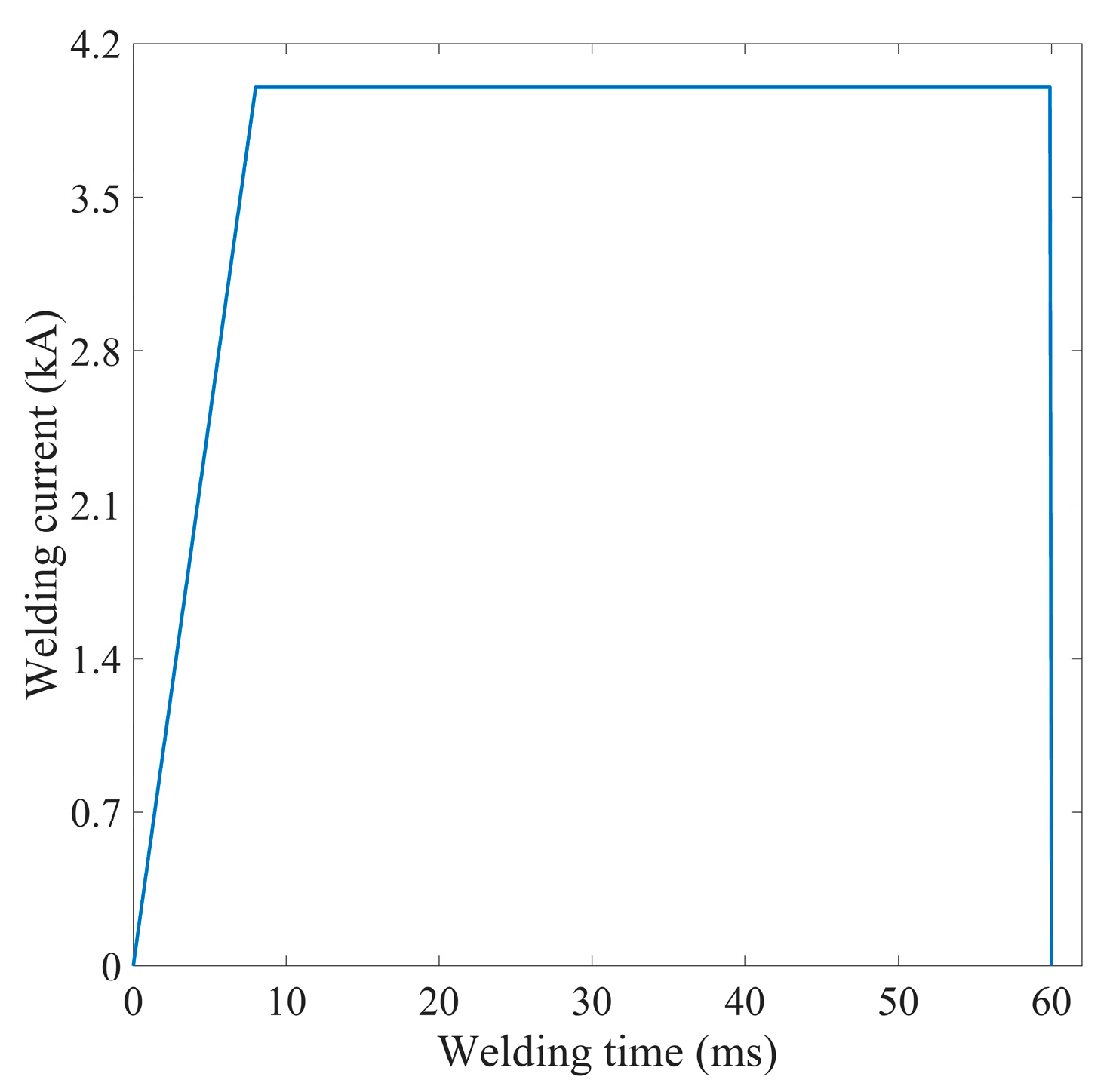
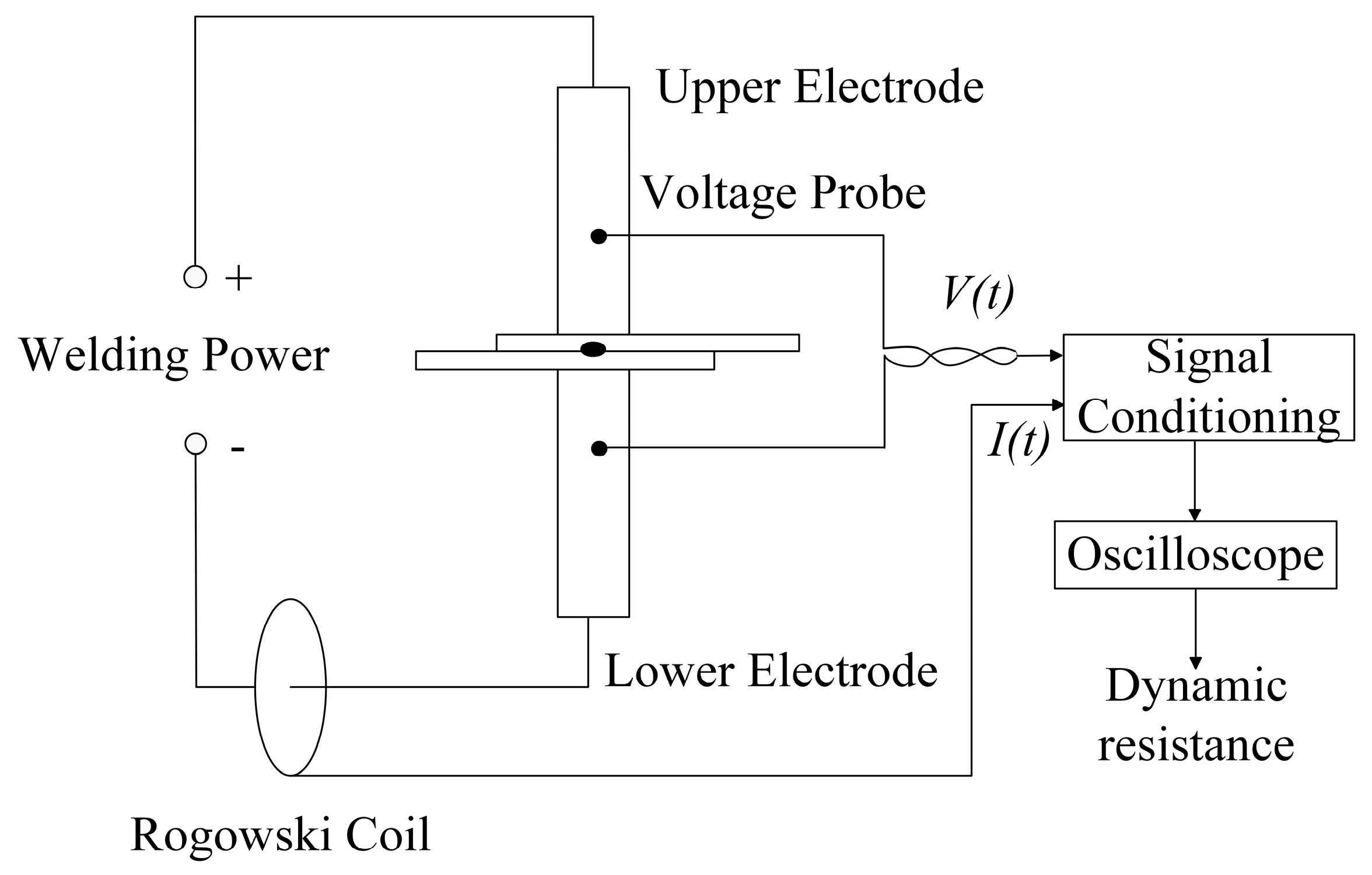
Figure 9 show the inter-electrode voltage and welding current signals as the 20th weld point is welded. At this time, the corresponding welding current is 4 kA, the welding time is 60 ms and the electrode pressure is 360 N. A medium frequency direct current resistance spot welding machine is utilised for this purpose. This ensures that the current variation during the welding process is very small, in contrast to the alternating current spot welder. Therefore, the dynamic resistance signal during the welding process can be obtained directly from Ohm's law.
where
R(
t) is the dynamic resistance,
U(
t) is the voltage,
I (
t) is the welding current and
t is the welding time.
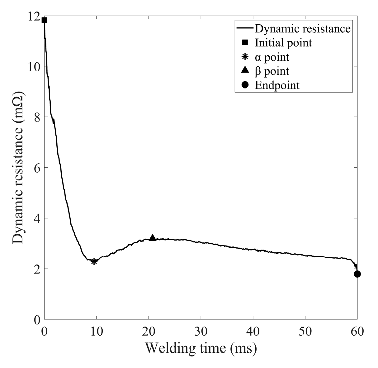
Figure 10 shows the dynamic resistance signal of the 20th weld. In general, the change in dynamic resistance with welding time can be divided into three stages. First, the welding current gradually increases from a very low value to 4kA and stabilises at this value. The upper and lower welding plates generate contact resistance affected by electrode pressure. The contact resistance generates heat and causes the contact surface of the welding plate to soften when exposed to the welding current. The contact area of the upper and lower steel plates increases, the contact resistance decreases and the dynamic resistance value decreases until it reaches the α point. After the upper and lower metal plates are in close contact, the temperature of the welded area increases under the effect of resistance heat. As a result, the resistivity of the BH 340 steel plate increases and when the temperature reaches the melting point of the metal, the metal melts. At this stage, the dynamic resistance increases until it reaches the β point. This point means that the metal in the weld area has melted to a certain extent and the liquid nugget has reached a certain size. Next, the energy dissipated by the electrode exceeds the heat created by the welding current and the dynamic resistance decreases again until it reaches the end point.
The basic objective of this study is to construct a robust model to quantitatively approximate the true functional relationship between the dynamic resistance signal and the electrode tip diameter in the non-stop resistance spot welding process, focusing on the mapping relationship between the dynamic resistance signal and the electrode tip diameter. Therefore, it is very necessary to first correlate the dynamic resistance curve with the electrode tip diameter. However, a dynamic resistance curve contains hundreds of data, so it is necessary to extract the most important data to achieve dimensionality reduction.
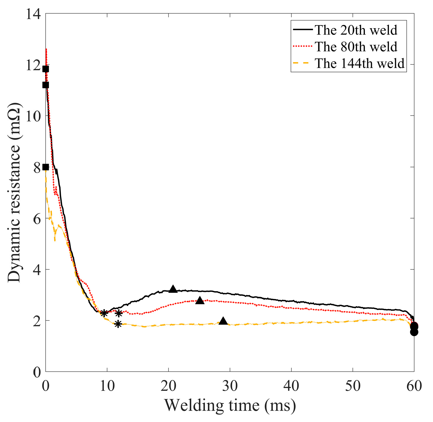
Figure 11 shows the evolution of the dynamic resistance signal when repeated at different welding times. This figure clearly shows that the dynamic resistance signal changes regularly as the number of joints increases. The resistance value at the β point gradually decreases and the welding time to reach this value is delayed accordingly. The overall dynamic resistance curve shows a downward trend as the number of joints increases, which is caused by the increasing electrode tip diameter due to electrode wear and the resulting decrease in welding current density [
24]. This finding is consistent with previous research showing that an increase in electrode tip diameter is an indication of electrode wear [
5]. When electrode wear is severe, the welding current density will decrease and the resulting heat will also decrease. At this point, the heating rate of the weld area is slower and it takes longer to reach the same welding heat as the previous weld point, so the time for the corresponding key points to appear is also delayed.
Figure 11 shows the trends as the number of welds increases. As the number of welding times increases from 20 to 144, the resistance value of the β point decreases from 3.57 mΩ to 1.84 mΩ and its appearance time is delayed by 19.56 ms. The same conclusion can be drawn from Ohm's law, welding heat is in direct proportion to the square of the welding current. If the density of the welding current is lower, it takes longer to reach a given welding heat. Bogaerts et al. [
25] discovered that the time to reach the β-point of the dynamic resistance is highly related to the heating rate during welding. It can be realised that the resistance value of the β point is also closely related to the corresponding welding time and the degree of electrode wear.
According to the change of dynamic resistance with the number of welded joints, some features can be extracted from the signal to express its changes. The positions of the α and β points and their resistance values are extracted. The final value of the resistance signal [
26] and the integral value of the dynamic resistance [
27] are also extracted. The slope between the four key points of the dynamic resistance (start point, α point, β point and end point) is also calculated.
Table 4 lists the 10 feature values extracted from the dynamic resistance signal.
3.3. Establishing models for the extracted features
Regression analysis, a quantitative statistical/computational technique, examines the functional relationship between independent variables and dependent variables in order to simulate and approximate the mapping relationship between them to the maximum extent. The regression model is obtained by analysing the relationship between the independent variables and the dependent variables using the method of least squares. Analysis of variance (ANOVA) was used as a tool to determine the significance and robustness of the regression model.
Assuming the independent variables (
) are continuous, their errors are small enough to be ignored. The functional relationship between the independent variables (
) and the dependent variable
y can be given by the following formula [
28]:
The functional relationship between independent and dependent variables requires a more accurate approximation. It is thus necessary to establish a regression equation to simulate the mapping relationship between them. The polynomial regression model is the most commonly used and its expression can usually be described as follows:
Where ε denotes the model error, xi represents each independent variable, indicates the dependent variable. The regression coefficient ai can be estimated from the obtained experimental data using the least squares regression method.
To investigate how the characteristics extracted from the dynamic resistance signal correlate with electrode size
D,
Table 5 expresses the correlation coefficient between them. This table clearly shows that the feature
k3 has the largest correlation coefficient with the electrode diameter of 0.882, while the feature
re of the dynamic resistance has the smallest correlation coefficient value. Features with correlation coefficients less than 0.5 were discarded and the remaining 9 features (
,
,
,
,
,
,
,
, and
) were used as inputs to the upcoming regression model to predict the electrode tip diameter (
D). The regression model was obtained using the stepwise regression analysis method and was obtained using MATLAB2017 software. The basic idea of the stepwise regression analysis method is to automatically select the most important variables from a large number of available variables and build a prediction model for regression analysis. The basic idea is to introduce the independent variables one by one, and the condition for introducing them is that the sum of squares of the partial regression is significant after testing. At the same time, each time a new independent variable is introduced, the old independent variables should be tested one by one, and the independent variables with insignificant partial regression sums of squares should be eliminated. In this way, variables are introduced and eliminated until no new variables are introduced and no old variables are eliminated. The 43 groups of data obtained from the welding experiment and the carbon printing experiment on carbon paper are divided into two groups: training samples and test samples. To obtain the regression model, 33 groups of all data were randomly selected as training samples, and another 10 groups of the test samples were used to verify the simulation accuracy and performance of the model. All regression and ANOVA results were performed on the average values of the two sets of data.
First, the regression model was constructed using the stepwise regression method based on the features extracted from the dynamic resistance signal. In this case, the Matlab software constructed different linear models according to the different data randomly selected each time. After many attempts, only the features of , and were retained, while other features like were discarded, even though they have high correlation coefficients with the electrode tip diameter.
Table 6 and
Table 7 show the ANOVA results of the linear regression model. If the P-value of the model and the terms included in the model are less than 0.1, it indicates that they are significant and should be retained. Otherwise, they should be discarded. Therefore, among the 9 features (
,
,
,
,
,
,
,
, and
) with a correlation coefficient with the electrode tip diameter greater than 0.5, only the extracted features
, and
are selected. By calculating the coefficient
R2, the adjusted
R2 and the sum of squared prediction errors, the fit of the regression model can be evaluated. A good regression model should have a coefficient of determination close to 1 and a small sum of squared prediction errors. The
R2 coefficient of this model is 0.9000, which implies that 90% of the experimental data agrees with the predicted data. The model only fails to predict the remaining 10% of the data. The adjusted
R2 is 0.8897, which is very adjacent to 0.9000 and also close to 1. Among the P-values of all the 9 features, only
, and
have P-values lower than 0.05, so the conclusion that can be drawn that they are highly significant [
29] and should be retained in this linear regression model.
To obtain a more accurate prediction model, a linear regression model with interaction terms was attempted to approximate the mapping relationship between the characteristic values of the dynamic resistance curve and the electrode diameter. The retained features extracted from the dynamic resistance curve (
,
, and
) and the interaction terms (
,
, and
) between them are used as independent variables in the regression model, and the electrode tip diameter
D is the dependent variable. The stepwise regression method was used, and Matlab 2017b software was used to construct a linear regression model with interaction terms. The results of the variance analysis of this model are illustrated in
Table 8 and
Table 9. This linear regression model is very significant as its P-value is much lower than 0.05.
R2 and adjusted
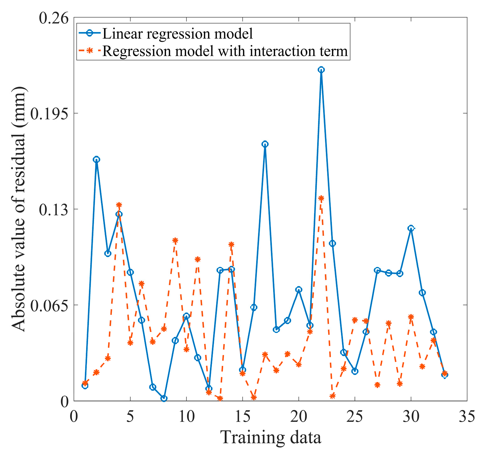
R2 are very similar and close to 1, and their values are higher than those of the first linear model. In such a case, the linear regression model with interaction terms is more accurate in predicting the electrode diameter.
Figure 12 is a good illustration of this statement. The graph reflects that the residual error of the second model is smaller.
In accordance with the results of the analysis of variance, the two regression models can be depicted as follows:
where
D is the electrode diameter,
r0,
P and
k3 are the features extracted from the dynamic resistance.
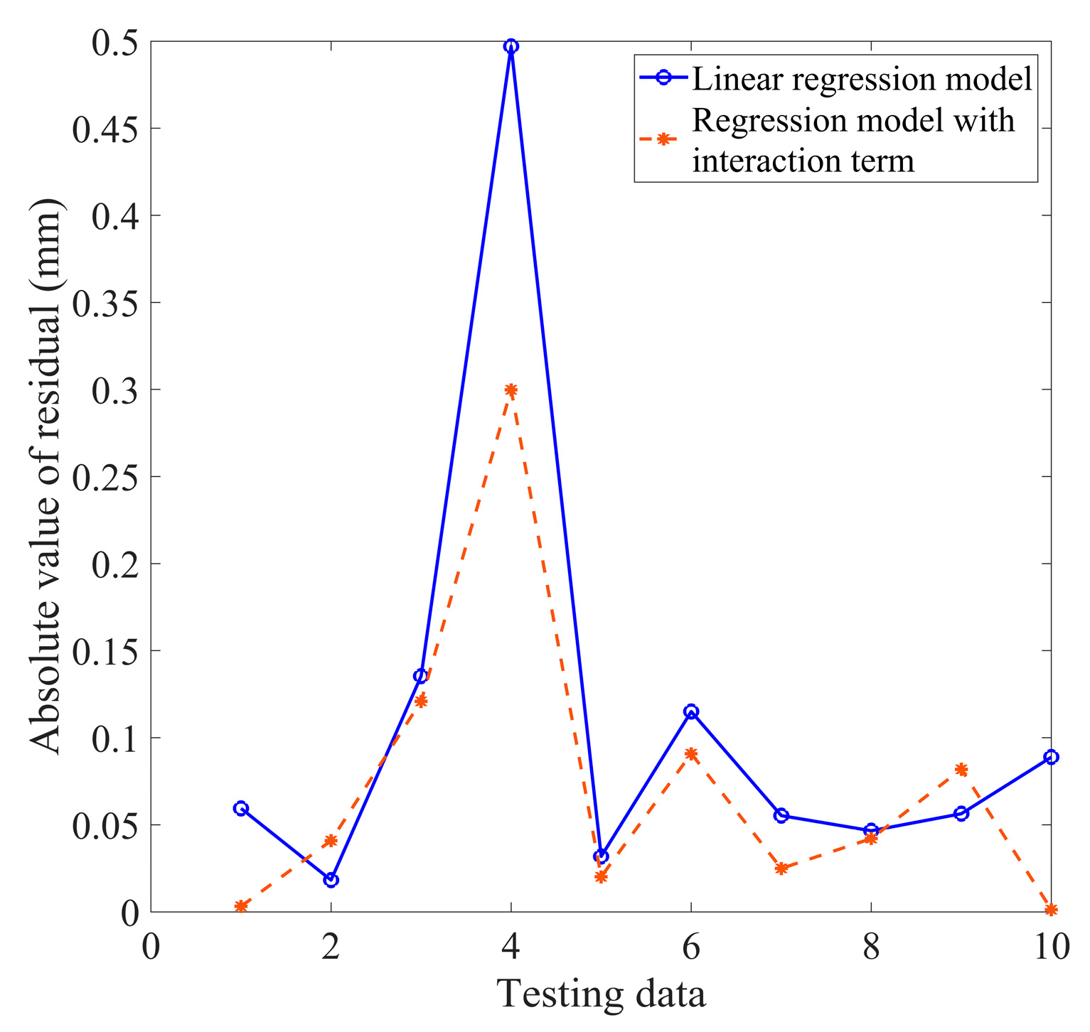
The prediction accuracy of the linear regression model and the linear regression model with interaction terms is shown in
Figure 13. This result is obtained using the 10 groups of testing data. The maximum prediction error of the linear regression model with interaction terms is 0.30 mm, while the maximum prediction error of the linear regression model is 0.50 mm. The corresponding relative prediction errors are 7.69% and 12.75% respectively, as revealed in
Table 10. It is not difficult to see that the linear regression model with interaction terms has a more accurate ability to evaluate and predict the electrode tip diameter than the linear regression model. In this circumstance, it is highly recommended to use a linear regression model with interaction terms related to selected features of the dynamic resistance curve to predict the electrode tip diameter. In such a case, monitoring dynamic resistance signals to obtain changes in electrode diameter can be an effective method of assessing the extent of electrode wear in practical production applications.
The subject of this study is closely related to trends in the automotive industry. Therefore, a complete and critical evaluation of the proposed solution in terms of suitability under real welding conditions and some editorial corrections are required. In this case, in order to verify the reliability of the prediction model proposed in this article for predicting the variation of the tip diameter of resistance spot welding electrodes with the number of welding points, it is planned to use a pair of new electrodes and perform continuous welding under the same welding conditions mentioned in
Section 2. The same test method is used to obtain the electrode tip diameter. The number of welding times is 54 and the electrode tip diameter is tested every few welds.
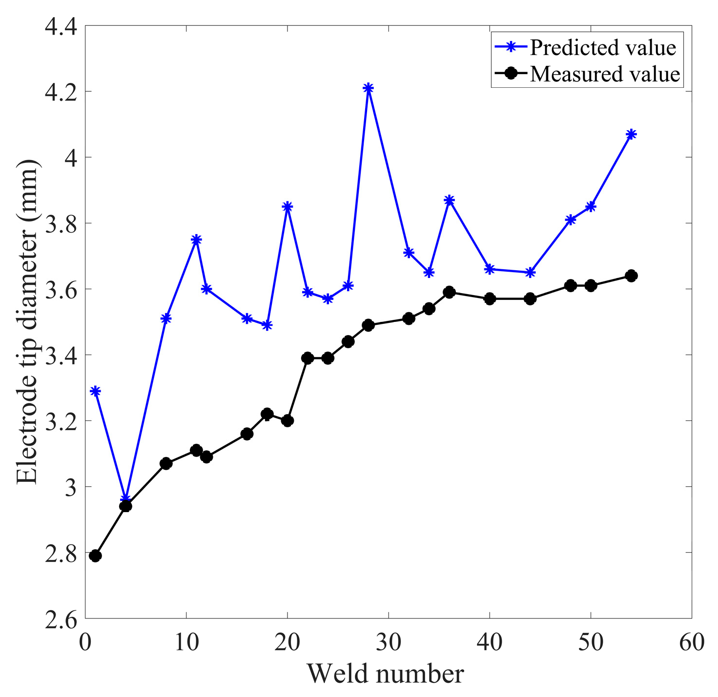
Figure 14 displays the predicted electrode tip diameter and the measured value using the linear regression model with interaction terms shown in equation (5).
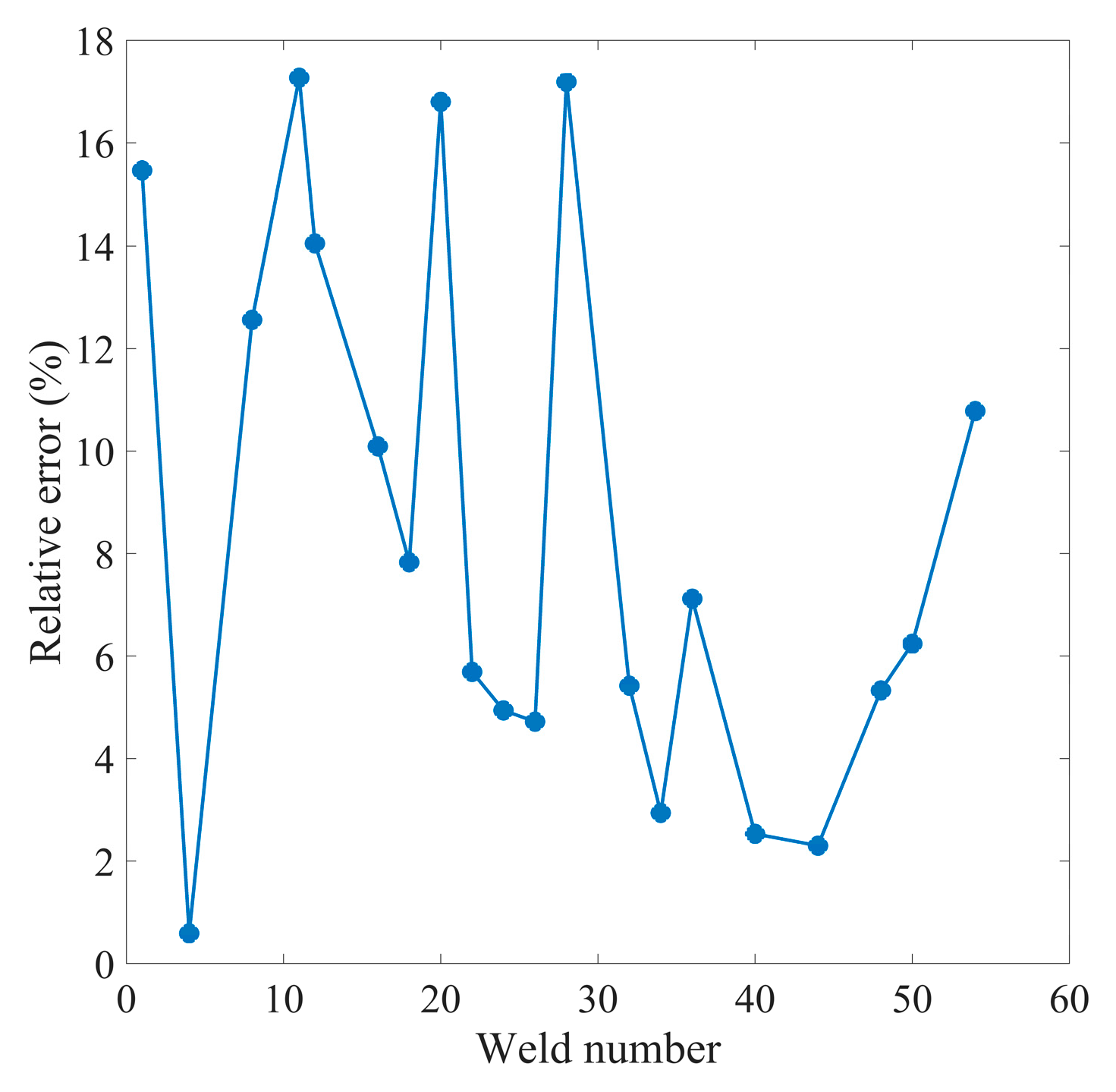
Figure 15 shows the relative error of the model prediction.
Table 11 lists the statistical values of the model prediction residuals.
The results show that, unexpectedly, the predicted values from the model are greater than the measured values. This implies that the model using dynamic resistance to predict electrode wear is more conservative, i.e. when the wear of the spot welding electrode actually reaches the critical point of its life, the model predicts that it has failed and the electrode needs to be replaced or repaired. On the one hand, this is more conservative in terms of ensuring the quality of the joint, but on the other hand it may result in wasted electrodes. Furthermore, the relative error of the model predictions is within 20%. The maximum absolute error is 0.72 mm. This indicates that the performance of the regression model in the welding situation of completely new electrodes is acceptable, but not fabulous.
The linear model with interactions built from the stepwise regression clearly overestimates electrode degradation and appears to be very sensitive to small variations in the dynamic resistance curve. The global tendency of the model follows the overall degradation of the electrode. Some of the possible reasons, how to address these and what needs to be done in the future include the following
1). As only 33 data sets were used to build the regression model in this article, the optimal regression model might not be obtained due to the limited data size. Therefore, future attempts to expand the data scale and use the average value obtained from multiple measurements to build a regression model are expected to perform better when faced with completely new data. In such a case, the reliability of the model will be improved by constructing a more complete database with several endurance tests and training the stepwise regression model on this database.
2). The method of manually extracting features from dynamic resistance curves is often based on experience and is highly subjective. The characteristic values selected often vary from person to person and very important characteristic values may be missed. Dimensionality reduction methods such as principal component analysis [
30] and deep learning algorithms [
31] can extract feature values according to certain rules, so they are expected to solve this problem.
3). The functional relationship between the characteristic values extracted from the dynamic resistance signal and the electrode tip diameter may be a very complex non-linear relationship, so simply using a linear regression model with interaction terms is not sufficient to simulate the complex mapping relationship between them. Intelligent algorithms such as artificial neural networks have the ability to approximate any non-linear mapping [
32], so the use of this artificial intelligence algorithm is expected to solve this problem.
4). Some researchers use the better non-linear function approximation capability of artificial neural networks and combine it with the stepwise regression analysis method to predict the observed variables of interest [
33]. Therefore, it is possible to obtain more satisfactory results by using the methods based on previous publications and applying them to electrode wear prediction.
In the future work, we will carry out tests on an actual production line to compare the estimated and measured electrode tip diameters over the entire electrode life (i.e. from 0 to XXX welds) to verify the accuracy of the developed new model over the entire electrode life.
