Data Augmentation for Regression Machine Learning Problems in High Dimensions

Preprint

Article

Data Augmentation for Regression Machine Learning Problems in High Dimensions

Altmetrics

Downloads

Views

Comments

A peer-reviewed article of this preprint also exists.

Clara Guilhaumon^*,Nicolas Hascoët,

Francisco Chinesta,Marc Lavarde,

Fatima Daim

Clara Guilhaumon^*,Nicolas Hascoët,

Francisco Chinesta,Marc Lavarde,

Fatima Daim

This version is not peer-reviewed

Submitted:

01 December 2023

Posted:

01 December 2023

You are already at the latest version

Alerts

Abstract

Machine learning approaches are currently used to understand or model complex physical systems. In general, a substantial number of samples must be collected to create a model with reliable results. However, collecting numerous data is often relatively time-consuming or expensive. Moreover, the problems of industrial interest tend to be more and more complex and depending on a high number of parameters. High dimensional problems intrinsically involve the need of large data amount through the curse of dimensionality. That is why, new approaches based on smart sampling techniques are investigated to minimize the number of samples to be given to train the model, such as Active Learning methods. Here, we propose a technique based on a combination of Fisher information matrix and of Sparse Proper Generalized Decomposition that enables the definition of a new Active Learning informativeness criterion in high dimensions. We provide examples proving the performances of this technique on a theoretical 5D polynomial function and on an industrial crash simulation application. The results prove that the proposed strategy over-perform the usual ones.

Keywords:

Subject: Computer Science and Mathematics - Artificial Intelligence and Machine Learning

1. Introduction

In the context of multi-parametric problems where one wants to estimate an output value Y that depends on multiple input variables,

X = (x_{1}, . . ., x_{n})

it is usual to resort to Machine Learning [1]. To do so, an algorithm is trained on a few examples grouped as a training database

(X_{t r a i n i n g}, Y_{t r a i n i n g})

to be able then to make predictions for unknown cases

X_{t e s t}

. The design of the training database is a main issue because it partly determines the performances of the algorithm (i.e. the further predictions). However, the generation of training samples if often costly. For instance, it can be really time-consuming to run simulations or to realize experiments. It can also be relatively expensive because of the cost of access to servers or machines.

Moreover, as the problems considered nowadays become more and more complex, and depend on a lot of input parameters, the models need a lot of samples to be trained. This issue is known as “curse of dimensionality” [2]. Indeed, the volume of the space increases so fast that the data become sparse and the number of necessary points needed to approximate the space increases too. Therefore, for these reasons, the samples employed by the algorithm need to be chosen efficiently.

Usually, training database are constructed thanks to the methodology of Design of Experiments [3]. Therefore, another approach has been developed over the past few years with the emergence of Active Learning [4]. This technique proceeds by iteration and lies on the assumption that, adding at each step the sample that improves the most the model will increase the performances quickly. Different ways to evaluate informativeness of a sample regarding a specific model have been investigated. Then, various corresponding information criteria have been defined for classification and regression. Nevertheless, a lot of them failed when it comes to operate in high dimensional settings.

Thus, we aim here to develop an efficient, iterative and automatic method to design a training set for high dimensional regression problems. To address this issue, a new information criterion from a combination of the information given by the Fisher matrix [5] with a Sparse Proper Generalized Decomposition (s-PGD) [6] has been defined. The proposed methodology is described in the Section 2. It will be then tested on two different applications, a polynomial function and a crash simulation problem. The results obtained are presented in Section 3. Finally, the paper is completed with some concluding remarks in Section 4.

2. Methodology

To tackle the issue of high dimensional regression problem, a new method for designing training databases has been defined following the steps of an Active Learning methodology. This method is based on the combination of the properties from the Fisher information matrix and a Model Order Reduction method through the use of s-PGD.

2.1. Active Learning

Firstly, various ways to design training databases for Machine Learning problems exist. One of the most classic ways to build these training databases is to resort to Design of Experiment (DOE) [3]. Indeed, DOE enables to better organize the tests done in scientific research or industrial studies. Their objective is to extract the maximum information with a minimum number of experiments and there are different ways in the literature to construct these plans such as : Full design [7], full factorial design [8], Plackett-Burman [9], Latin Hypercube Sampling [10]...

However, their major disadvantage is that their conception only depends on the input space and does not take into consideration the output. Moreover, the number of data needed depends on the number of dimensions and levels chosen. Thus, it often increases drastically with the number of dimensions, suffering from the “curse of dimensionality” [2]. That is why, other iterative and automatic methods have subsequently been developed, like Active Learning methods [4].

The main idea of Active Learning, is sum up in Figure 1. A Machine Learning algorithm will be able to achieve better performances with few training samples if it can choose the data from which it will learn. Therefore, the algorithms ask at each step for the real output value associated with a sample “query” that an external entity named “oracle” must then provide. It stops when the objective had been reached according to a stopping criterion.

As a result, Active Learning is particularly suitable in many current Machine Learning problems, where data can be time-consuming or expensive to obtain.

2.1.1. Scenarios

In Active Learning, there are different scenarios in which the queries can be made. Indeed, there are different ways to select or take a sample in order to add it to the training database of the trained model. That is why, a quick overview of the query strategies proposed in the literature will be presented here.

The three main methods described in the literature and detailed after are: (i) Membership Query Synthesis [11,12,13], (ii) Stream-Based Selective Sampling [14], and (iii) Pool-Based Sampling [15].

(i): Membership Query Synthesis [11]: Here, the model can ask for any sample in the input space, it can also ask for queries generated de novo rather than for those sampled from an underlying natural distribution. This method has been particularly effective for problems confined to a finite domain [12]. Initially developed for classification models, it can also be extended to regression models [13]. However, this method may leave too much freedom to the algorithm which can be led to request samples without any physical meaning.
(ii): Stream-Based Selective sampling [14]: Here, the initial assumption is that it is not expensive to add a sample. Therefore, the model decides for each possible sample whether to add it as training data. This approach is also called sometimes Stream-Based or Sequential Active Learning because all the samples are considered one by one and the model chooses for each one whether to kept or not.
(iii): Pool-Based Sampling [15]: There, a small set L of labelled data and a large set denoted U of unlabelled available data are considered. The query is then made according to the information criterion which evaluates the relevance of a sample from the basis U in comparison to the others. The best sample according to this criterion is then chosen and added to the training set. The difference with the previous scenario is that the decision regarding a sample is taken individually. In the Pool-Based the others samples still available are taken into account. This last method is the most used in real applications.

Next, to assess the relevance of a sample and to be able to apply these scenarios, it is necessary to quantify the information carried by a sample.

2.1.2. Query strategies

The quantification of the information carried by a sample can also be diverse and has led to the definition of various query strategies in the literature. The notation

x_{A}^{*}

refers to the most informative sample (i.e. the best or most relevant sample) for each of given method A. The input values are noted x, the outputs

y_{i}

range over all possible labelling i, and the model estimation

θ

Uncertainty Sampling Uncertainty sampling [15,16,17,18] considers that the most informative sample is the one the model is most uncertain to predict correctly. With the entropy definition from [18] this uncertainty can be written:

$x_{U S}^{*} = arg max_{x} \sum_{i} P_{θ} (y_{i} ∣ x) l o g P_{θ} (y_{i} ∣ x)$

(1)
Query by Committee A committee of models trained on different hypothesis on the base L is defined $C = \{θ^{(1)}, . . ., θ^{(C)}\}$ . Then, a vote is done and the sample which generates the most disagreement is selected and added [19]. There are different ways to measure the level of disagreement and make the final vote. The two most used are: the vote entropy described in [20] and the Kullback-Leibler (KL) divergence in [21].
Expected model change For a given model and a given sample, the impact of the sample if added to the training database L is estimated through a gradient calculation. The sample that induces the biggest change is here the most relevant and is added to the training [22,23] :

$x_{E M C}^{*} = arg max_{x} \sum_{i} P_{θ} (y_{i} ∣ x) ∥ \nabla l_{θ} (\{x, y_{i}\}) ∥$

(2)

where $\nabla l_{θ} (\{x, y_{i}\})$ is the gradient of the objective function l respectively to the parameters $θ$ applied to the tuple $\{x, y_{i}\}$
Variance reduction The most informative sample which will be added to the training set is the one minimizing the output variance (i.e. minimizing the generalization error) [24]:

$x_{V R}^{*} = arg min_{x} < σ_{\hat{y}}^{2} >^{+ x}$

(3)

where $< σ_{\hat{y}}^{2} >^{+ x}$ is the estimated mean output variance across the input distribution after the model has been re-trained on the query x and its corresponding label.

Thanks to theses various definitions of scenarios and queries strategies many methods of active sampling design can be settled up.

However, most of them don’t work effectively for high dimensional regression. Indeed, lots of criterion are defined with an euclidean distance

∥ x_{i} - x_{j} ∥

between

x_{i}

and

x_{j}

points of the input space. In high dimensions the distance between two points is high for any points. Therefore, the criterion has similar value for each point and can not be used.

2.2. s-PGD equations

On one hand, to deal with high dimensional problems a common solution is to resort to Model Order Reduction methods (MOR) [25]. These methods allow to reduce the computational complexity of mathematical models in numerical simulations. Indeed, even if using a reduced basis generates some loss of generality, it often allows impressive computing time savings. Moreover, if the problem solution is in the reduced basis, the calculated solution with MOR remains quite precise.

Various algorithms belong to the MOR field such as the Proper Orthogonal Decomposition (POD) [26], Principal Component Analysis (PCA) [27] ... One of these algorithms is the sparse Proper Generalized Decomposition (s-PGD) [6,28]. It is the one that will be used in this paper.

If we consider a function f in n dimensions:

f (x_{1}, . . ., x_{n}) : Ω \subset R^{n} \to R

(4)

Where

x_{1} . . . x_{n}

are the input variables, the s-PGD can be expressed as the following decomposition:

f (x_{1}, . . ., x_{n}) \approx {\tilde{f}}^{M} (x_{1}, . . ., x_{n}) = \sum_{m = 1}^{M} \prod_{k = 1}^{n} X_{m}^{k} (x_{k})

(5)

Then, X can be decomposed as :

X_{m}^{k} (x_{k}) = \sum_{j = 1}^{M} N_{j, m}^{k} a_{j, m}^{k} = {(N_{m}^{k})}^{T} a_{m}^{k}

(6)

Where M stands for the number of terms in the decomposition,

N_{j, m}^{k}

are the set of basis functions for the corresponding

k^{t h}

dimension and

m^{t h}

mode, and

a_{j, m}^{k}

are the coefficients for the corresponding

k^{t h}

dimension and the

m^{t h}

mode also.

These approximated functions

{\tilde{f}}^{M}

are calculated step by step thanks to a greedy algorithm and the new

M^{t h}

order term is found using a non-linear solver (Picard or Newton, for instance):

{\tilde{f}}^{M} = \sum_{m = 1}^{M - 1} \prod_{k = 1}^{n} X_{m}^{k} (x_{k}) + \prod_{k = 1}^{n} X_{M}^{k} (x_{k})

(7)

In a Machine Learning framework this approximation allows to make an estimation of the output values related to an unknown data. Moreover, achieving this is particularly difficult when confronted with a high-dimensional problem, where the data is sparse and/or scarce. Indeed, the regression problem described here only guarantees that the minimization is satisfied by the training. Thus, if the sampling points in the training set are not numerous enough, high oscillations may appear out of these measured points because the risk of over-fitting has increased. This affects the predictions of the generated model.

To deal with this issue, a Modal Adaptivity Strategy (MAS) can be settled up. The idea of MAS is to minimize the oscillations outside the training set by starting the PGD algorithm with only low degree modes. When the residual values then decrease slowly enough or reach a fixed value, higher order approximation functions are added. This method has proven to be an efficient way to improve the s-PGD performances in many cases [29,30,31,32]. However, some limits remain. For instance, it has been noted that the desired accuracy is not achieved before reaching over-fitting or the algorithm can stop too early when using MAS in some cases. In addition, in problems where just a few terms of the interpolation basis are present, the method fails in identifying the true model and leads to bad predictions.

To solve these difficulties, other versions of the PGD have been developed such as the rs-PGD and the s2-PGD as detailed in [28].

2.3. Fisher Matrix

On the other hand, to develop an Active Learning methodology it is necessary to define an informativeness criterion. Yet, one way to quantify the information quarried in a series of observations is to use Fisher information [5,33], or for n parameters, the corresponding Fisher information matrix.

If considered the likehood

f (X, μ)

a function of X with respect to parameter

μ

. In statistics the Fisher information is a way of measuring the information carried by an observable random variable about an unknown parameter

μ

of a distribution that models X.

Moreover, the main issue in defining a DOE, is the ease to identify parameters by maximizing the likehood. Indeed, where f is sharply peaked with respect to changes in

μ

, the data provides a lot of information about the parameter

μ

. Then, it is easy to indicate the "correct" value of

μ

from the data. On the contrary, if f is flat, many samples are needed to determine the actual parameters values with an adequate accuracy. Therefore, the variance with respect to

μ

could be a valuable indicator to optimize the design.

To do so, the partial derivative with respect to

μ

of the log-likehood formally called score s can be written as:

s (μ) = \frac{\partial log f (X, μ)}{\partial μ}

(8)

Then, the variance of the score is by definition the Fisher information

I

I (μ) = V (s (μ)) = E (s {(μ)}^{2}) - {(E (s (μ)))}^{2}

(9)

Under certain regularity conditions the first moment of the score vanishes,

\begin{matrix} E (s (μ)) & = E (\frac{\partial log f (X, μ)}{\partial μ}) = \int \frac{\frac{\partial f (x, μ)}{\partial μ}}{f (x, μ)} f (x, μ) d x \\ = \frac{\partial}{\partial μ} \int f (x, μ) d x = \frac{\partial}{\partial μ} 1 = 0 \end{matrix}

(10)

It gives,

I (μ) = E ({(\frac{\partial log f (X, μ)}{\partial μ})}^{2})

(11)

Which taking into account,

\frac{\partial^{2} log f (X, μ)}{\partial μ^{2}} = \frac{\frac{\partial^{2} f (X, μ)}{\partial μ^{2}}}{f (X, μ)} - {(\frac{\partial log f (X, μ)}{\partial μ})}^{2}

(12)

And

E (\frac{\frac{\partial^{2} f (X, μ)}{\partial μ^{2}}}{f (X, μ)}) = \frac{\partial^{2}}{\partial μ^{2}} \int f (x, μ) d x = 0

(13)

Yields

I (μ) = - E (\frac{\partial^{2}}{\partial μ^{2}} log f (X, μ))

(14)

When considering many parameters

μ = (μ_{1}, μ_{2} . . .,)

it results in the so-called Fisher information matrix, whose components read,

I_{i, j} (μ) = E ((\frac{\partial}{\partial μ_{i}} log f (X, μ)) (\frac{\partial}{\partial μ_{j}} log f (X, μ)))

(15)

i.e

I (μ) = E ((\nabla log f (X, μ)) {(\nabla log f (X, μ))}^{T})

(16)

2.4. Computation of a new information criteria

The previous definition of Fisher information (16) can be applied to any model of X. Then, it can be applied to a s-PGD decomposition (5).

For the ease of the exposition and without loss of generality, let us begin by assuming that the unknown objective function lives in

R^{2}

. If f is decomposed through s-PGD it gives for the first decomposition mode:

f = (F^{T} a) (G^{T} b)

(17)

Where

F = (F_{1}, . . ., F_{N})

and

G = (G_{1}, . . ., G_{N})

are the set of basis functions for the corresponding dimensions and

a

and

b

the corresponding vectors of coefficients.

Then, for a fixed value

a_{k}

a

and

b_{l}

b

\frac{\partial f}{\partial a_{k}} = F_{k} (G^{T} b)

(18)

\frac{\partial f}{\partial b_{l}} = G_{l} (F^{T} a)

(19)

Where

F_{k}

and

G_{l}

are the corresponding basis functions of

a_{k}

and

b_{l}

Thus, the derivative can be written as:

\frac{\partial f}{\partial μ} = (\begin{matrix} F_{1} (G^{T} b) \\ ⋮ \\ F_{N} (G^{T} b) \\ G_{1} (F^{T} a) \\ ⋮ \\ G_{N} (F^{T} a) \end{matrix})

(20)

Therefore,

\begin{matrix} I (μ) & = E ((\frac{\frac{\partial f (X, μ)}{\partial μ}}{f (X, μ)}) {(\frac{\frac{\partial f (X, μ)}{\partial μ}}{f (X, μ)})}^{T}) \\ = E (\frac{1}{f (X, μ) f {(X, μ)}^{T}} (\frac{\partial f (X, μ)}{\partial μ}) {(\frac{\partial f (X, μ)}{\partial μ})}^{T}) \end{matrix}

(21)

Finally, replacing with the derivative and with the variance noted

σ

\begin{matrix} I (μ) & = \frac{1}{σ^{2}} (\begin{matrix} F_{1} (G^{T} b) \\ ⋮ \\ F_{N} (G^{T} b) \\ G_{1} (F^{T} a) \\ ⋮ \\ G_{N} (F^{T} a) \end{matrix}) {(\begin{matrix} F_{1} (G^{T} b) \\ ⋮ \\ F_{N} (G^{T} b) \\ G_{1} (F^{T} a) \\ ⋮ \\ G_{N} (F^{T} a) \end{matrix})}^{T} \\ = \frac{1}{σ^{2}} (\begin{matrix} F F^{T} {(G^{T} b)}^{2} & F G^{T} (G^{T} b) (F^{T} a) \\ G F^{T} (G^{T} b) (F^{T} a) & G G^{T} {(F^{T} a)}^{2} \end{matrix}) \end{matrix}

(22)

Then, for a design of experiment of M samples

ξ = (ξ_{1}, ξ_{2}, . . ., ξ_{M})

, the information matrix is:

I (μ, ξ) \equiv \sum_{i = 1}^{M} I (μ, ξ_{i})

(23)

Finally, as demonstrated in the General Equivalence Theorem in [34], the equivalent variance on a new point

χ

is:

d (μ, χ) \equiv {(\frac{\partial f (μ, χ)}{\partial μ})}^{T} I (μ, ξ) \frac{\partial f (μ, χ)}{\partial μ}

(24)

This value d will be used as our new information criterion in the Active Learning Process. As it is an equivalent of the variance, we will seek for the point with the highest value of d. Then, we calculate its corresponding output

f (χ)

to add the point to the training data base.

The whole methodology to build the training database step by step according to this criterion is summed up in the following workflow.

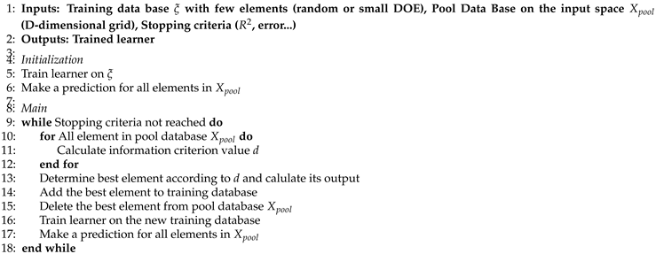
Algorithm 1 Active Learning : Matrix criterion

Finally, a sampling design method has been obtained and can be applied to high dimensional regression problem.

For a general s-PGD decomposition with more functions and modes the same idea can be extended. Some detailed calculations are shown in Appendix A.

3. Tests and results

In this section, the proposed method will be applied to two examples. First, one theoretical example with a polynomial function in a 5 dimensional space that is not well estimated using a simple DOE and s-PGD. Secondly, one industrial crash simulation application.

The results obtained on these two applications have been compared to the ones computed with more usual, or previously used, sampling methods.

3.1. Polynomial function

As a first example, we are trying to estimate the following polynomial function from [28] in a 5 dimensional input space.

\begin{matrix} f (x & = (x_{1}, x_{2}, x_{3}, x_{4}, x_{5})) \\ = {(8 x_{1}^{3} - 6 x_{1} - 0.5 x_{2})}^{2} + {(4 x_{3}^{3} - 3 x_{3} - 0.25 x_{4})}^{2} + 0.1 (2 x_{5}^{2} - 1) \end{matrix}

(25)

In Figure 2, a plot of the ground truth function is shown for

f (x_{1}, x_{2}, x_{3} = 0, x_{4} = 0, x_{5} = 0.7071)

as in [28] for comparison purpose.

The function is considered on the input space

Ω = {[- 0.5, 0.5]}^{5}

, and the predictions are made over this space using an s-PGD model trained with the Fisher Matrix Active Learning method. The results are compared with an s-PGD trained on an LHS with the same number of samples as training database and with the results of the previous article [28], which are obtained through a 4-th order MAS s-PGD, and an LHS of 160 points as training set.

Moreover, for the Matrix Method the next sample is chosen within a pool of available samples like in a pool-based strategy. This pool is defined as a k-dimensional grid (5 here) of N subdivisions, which gives a group of

N^{k}

possible elements evenly distributed over the input parametric space. In our application, a refined research grid of size

20^{5}

is used to have a wide choice of queries.

In Figure 3, the output shape of the function is plotted at different steps for the same fixed parameters as before. The blue points are the initial training points for the model at this step. The red ones are the new added points for different number of queries. On the left side the samples are computed with the Matrix Method. On the right side, new samples are computed using LHS.

With the Matrix Method, the training points are added accordingly to the shape of the predicted output function and in order to reduce the output variance. This leads to more points on the curved areas and borders, while the LHS gives a more random and evenly distributed screening on the input space independent of the output shape. As shown in Figure 3, the prediction is adapted step by step in the Matrix Method until no more significant change. This precision can be settled accurately by adapting the value of the stopping criterion.

To compare more directly the performances of both methods, the correlation coefficients, defined as follows in Equation (26) and calculated on the test set, are evaluated.

R^{2} = \frac{\sum_{i = 1}^{n} (Y_{p r e d, i} - \bar{Y_{p r e d}}) (Y_{t r u e, i} - \bar{Y_{t r u e}})}{\sqrt{\sum_{i = 1}^{n} {(Y_{p r e d, i} - \bar{Y_{p r e d}})}^{2}} \sqrt{{(Y_{t r u e, i} - \bar{Y_{t r u e}})}^{2}}}

(26)

Where

Y_{p r e d}

corresponds to the prediction made by the model,

Y_{t r u e}

to the real output values and

\bar{Y_{p r e d}}

\bar{Y_{t r u e}}

to the corresponding means.

The results, from 25 to 55 queries, for both LHS and Matrix Method at each step are plotted in Figure 4. These plots have been repeated for 400 iterations of the whole Active Learning process with different initialization databases (constructed with different LHS of 25 values). The average, first and last quartile of

R^{2}

have been extracted for each method.

It appears that the Matrix Method converges faster than the LHS, reaching a stable level with a training database of 40 samples, while the LHS performances are still increasing and lower. Adding samples increasingly gives an average correlation value of 0.824 while it only reaches 0.647 with an LHS for 35 samples. Compared to the results of the previous study in [28], where a training of an LHS with 160 samples has been chosen to reach an

R^{2}

of 0.88, here the same value can be obtained with only 35 samples.

Besides, it is also noteworthy that the initial training database has a lot of impact on the results. Specially at the beginning of the Active Learning process. Indeed, the interquartile range is, at first, around 0.23 for the Matrix Method and 0.21 for the LHS, meaning the dispersion is notable. After that, it decreases quickly for the Matrix Method, reaching 0.07 against 0.5 for the LHS around 10 queries. This phenomenon is explained because the LHS seeks to increase the inertia by starting in random directions. This is optimal for a group of tests, but the estimator does not take into account the past training data. On the contrary, our approach, is sought to optimize the points and the past sets of points with a criterion of minimization of the variance.

Moreover, the grid size can be more or less refined and needs a compromise. Indeed, this is illustrated in Figure 5 where the final value of

R^{2}

after 30 queries is plotted. That is to say after the criterion has converged and no more variation between the queries at the state n and

n + 1

. This shows that with a wider grid size the

R^{2}

values obtained by the Matrix Method can be higher and thus the performances obtained by the model are better. For example, for 35 queries a

R^{2}

value of 0.790 is obtained for a

10^{5}

grid against 0.824 for a

20^{5}

grid.

This can be easily explained because with a more refined grid more “next points” are available, and the algorithm can choose more precisely where to add a new point. However, it is also more time consuming to compute the criterion for the whole grid, and it is more memory consuming to save and calculate the corresponding values. Thus a compromise is necessary. Moreover, it appears in Figure 5 that after 10 subdivisions the slope of increase is lower. For this problem a subdivision after 10 should be chosen, still taking into account the calculation time.

Globally, the results obtained with the Matrix Method appear to be significantly better than with usual samplings. Although at first it is more time-consuming, or computationally more expensive, to determine the next point to add at each step, time and costs are saved in the end because fewer amount of samples are required by the model to converge. This aspect is particularly interesting for industrial applications where simulation or experimental costs need to be minimized.

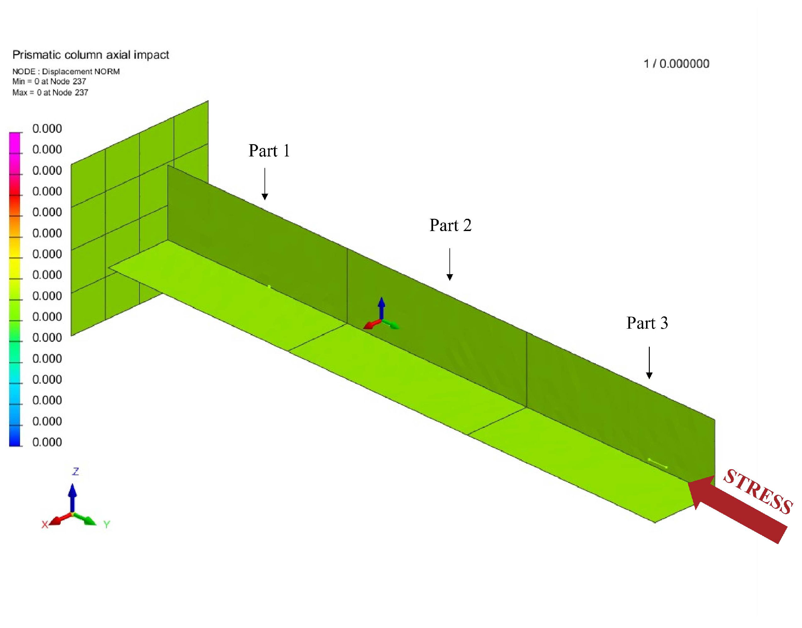
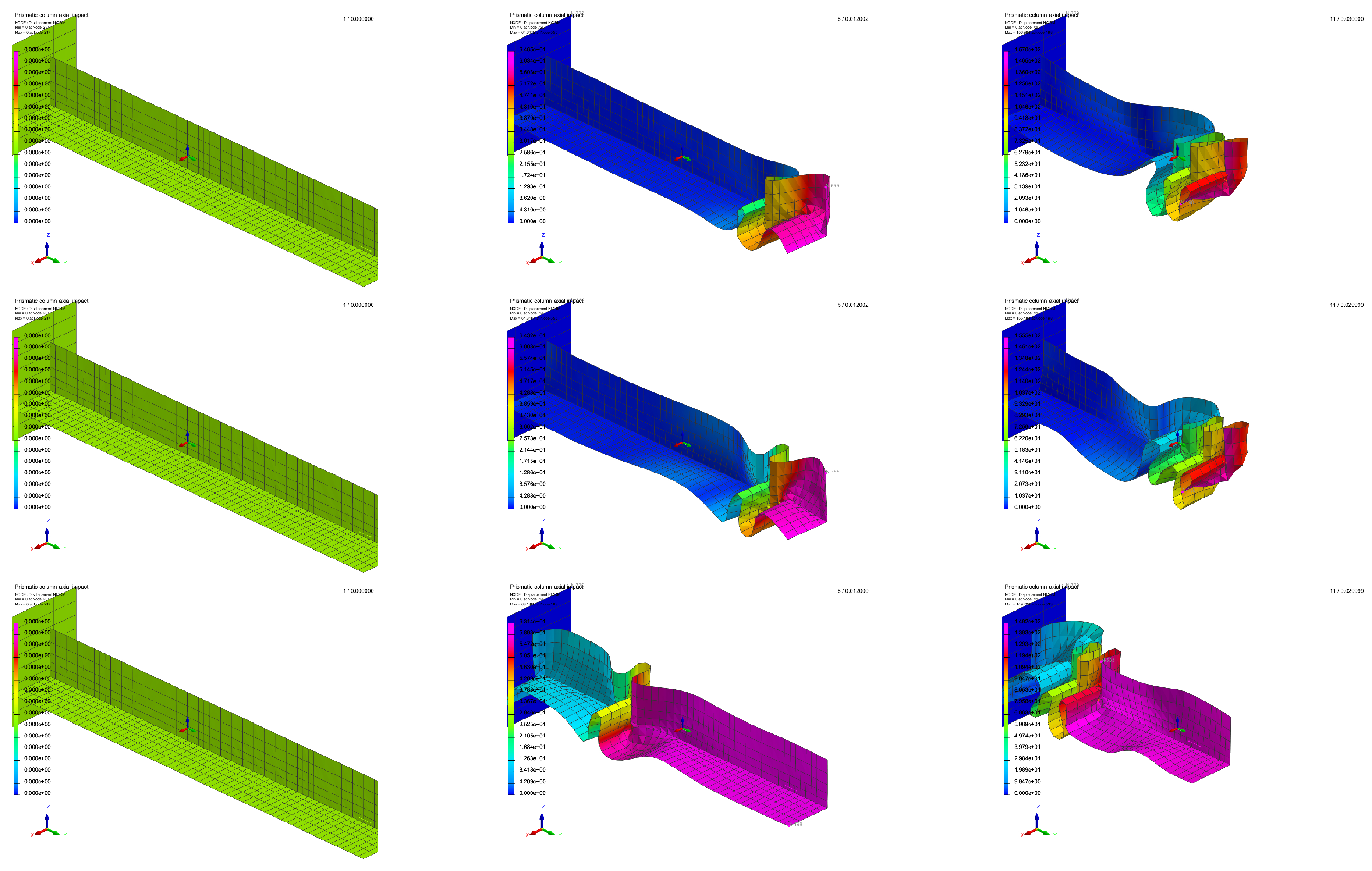
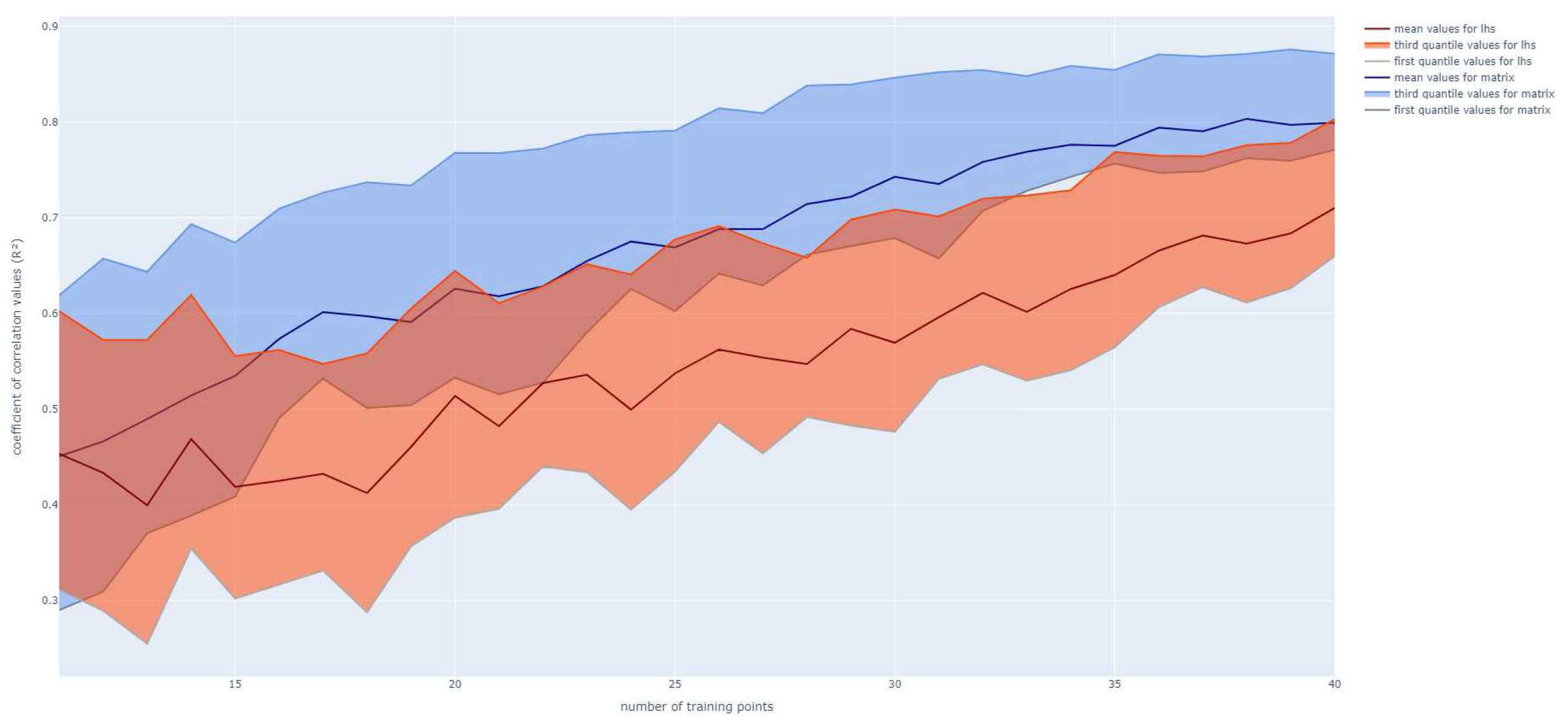
3.2. Application on a box-beam crash absorber

Now, this method was applied to an industrial mechanical problem through a box-beam deformation example. The idea, here, is to study and predict the deformation of a beam separated in tree parts. Each part (part 1, part 2 and part 3) has a specific thickness. The whole beam is subjected to a loading along its main axis

(y)

on one side and clamped on the other. The model is represented in Figure 6.

The application of the stress smashes the beam along the y axis. The corresponding deformation depends on the thickness chosen for the tree boxes. Some cases are represented in Figure 7. First, intermediate and last time step for different inputs values of thicknesses for the 3 parts are illustrated.

In this case, the model’s aim is to estimate the displacement along the main axis of a point located at the edge of the beam at the final simulation time step function of the thicknesses chosen for each box as input parameters

(h_{1}, h_{2}, h_{3})

. As before, we will compare the performances (in terms of

R^{2}

values) for s-PGD models trained with our active method and with an LHS with the same number of samples. As only 3 parameters are involved here, the initialization for the Matrix Method is done with a small LHS of 10 samples.

Moreover, the whole process is repeated 100 times to make an average of the results obtained, which is plot in Figure 8.

The grid is refined with a

3^{50}

size to be precise enough.

It appears in Figure 8 that as for the previous example, the Matrix Method reaches higher values of

R^{2}

faster than the use of an usual DOE. Indeed, it gives in average a value

12 %

higher than with the LHS. However, the increase of the two methods is here more similar than before. The difference is also less important. This can be explained because there are only three parameters involved and the behaviour of the output is quite simple. There is also still a variability associated to the initialization state, with a

19 %

of average variation for the Matrix Method and

22 %

for standard LHS.

4. Conclusion and future works

To sum up, a new information criterion was proposed to determine which sample would be the most valuable to add to the training database of a high-dimensional regression model to improve its performances step by step. The results of this method appear to be quite conclusive. Indeed, the precision of the predictions function of the number of samples in the training database increases faster with this method, than with more usual DOEs (such as LHS). Moreover, this criterion does not only depend on the shape of the input space, but also takes into account the output values. This way, the models are automatically refined where there are variations in the output space and can adapt faster to a specific problem.

However, this methodology can still be improved in different ways:

First, the samples, in this study, are added one by one, but it could be interesting to add them by group. Indeed, it seems that the algorithm needs to select some points in the same area to estimate it before moving to others. This behaviour can be explained because the information criterion used aims to minimize the global output variance. Adding points by group could be an interesting way to solve this issue. In further studies, studying how and how much points to add would be relevant. Moreover, when the real output value (given by the “oracle”) comes from experiments, it is more pertinent to do more than one point simultaneously to have a better organization.
Another point that could be optimized, is the search of the criterion optimum value. As for now, a simple research along a refined grid is used. Using an optimized method to find optimum (such as a gradient descent for example) or using an adaptive grid mesh which would refine itself near the interesting areas could be an option. This is also interesting in a purpose of reducing the computational cost of the algorithm. Indeed, searching precisely without generating a huge grid will be a good improvement and should be optimized.
In terms of practical use, developing an algorithm to determine and maybe adapt during the whole active learning process the s-PGD parameter (number of modes, function degrees) would also improve the speed of convergence.
Finally, the mix of the criterion with a more specific cost function is also considered to improve the results as it was studies in the preliminary’s step of the method development.

In the end, let’s highlight that the matrix method criterion is particularly efficient for high dimensional problems. Indeed, unlike usual active learning regression criterion it does not depend on any distance. This will be confirmed by applying this new methodology for a much higher dimensionaly problem.

Author Contributions

Conceptualization, F.C. and M.L.; methodology, N.H. and C.G.; validation, N.H., C.G. and F.D.; investigation, F.C., M.L., N.H. and C.G.; resources, F.D.; writing—original draft preparation, C.G.; writing—review and editing, N.H., F.C.and M.L.; supervision, N.H., F.C. and M.L.. All authors have read and agreed to the published version of the manuscript.

Funding

This research received no external funding

Institutional Review Board Statement

Not applicable

Data Availability Statement

Data supporting the findings of this study are available from the corresponding author upon reasonable request.

Conflicts of Interest

The authors declare no conflict of interest.

Appendix A. Matrix method criterion detailed definition

Let us consider an unknown function whose approximation is precisely the objective of this work. A function f depending of n input variables

x_{1}, x_{2}, . . ., x_{n}

such as:

f (x_{1}, x_{2}, . . ., x_{n}) : Ω \subset R^{n} \to R

(A1)

With s-PGD it can be also written as:

f (x_{1}, . . ., x_{n}) \approx {\tilde{f}}^{M} (x_{1}, . . ., x_{n}) = \sum_{m = 1}^{M} \prod_{k = 1}^{n} X_{m}^{k} (x_{k})

(A2)

The modes will be noted m, the degrees of the functions d, the dimensions k and

X_{m}^{k}

and

N_{d}^{k}

are the decomposition vectors.

The corresponding vector for an example where

m = [1, 2]

d = [1, 2]

and

k = [1, 2, 3]

can be written:

J (μ, x_{1}, x_{2}, x_{3}) = (\begin{matrix} m = 1, d = 1 \{\begin{matrix} k = 1 \\ k = 2 \\ k = 3 \end{matrix} & (\begin{matrix} N_{1}^{1} (x_{1}) X_{1}^{2} (x_{2}) X_{1}^{3} (x_{3}) \\ N_{1}^{2} (x_{1}) X_{1}^{2} (x_{2}) X_{1}^{3} (x_{3}) \\ N_{1}^{3} (x_{1}) X_{1}^{2} (x_{2}) X_{1}^{3} (x_{3}) \end{matrix}) \\ m = 2, d = 1 \{\begin{matrix} k = 1 \\ k = 2 \\ k = 3 \end{matrix} & (\begin{matrix} N_{1}^{1} (x_{1}) X_{2}^{2} (x_{2}) X_{2}^{3} (x_{3}) \\ N_{1}^{2} (x_{1}) X_{2}^{2} (x_{2}) X_{2}^{3} (x_{3}) \\ N_{1}^{3} (x_{1}) X_{2}^{2} (x_{2}) X_{2}^{3} (x_{3}) \end{matrix}) \\ m = 1, d = 2 \{\begin{matrix} k = 1 \\ k = 2 \\ k = 3 \end{matrix} & (\begin{matrix} X_{1}^{1} (x_{1}) N_{2}^{1} (x_{2}) X_{1}^{3} (x_{3}) \\ X_{1}^{1} (x_{1}) N_{2}^{2} (x_{2}) X_{1}^{3} (x_{3}) \\ X_{1}^{1} (x_{1}) N_{2}^{3} (x_{2}) X_{1}^{3} (x_{3}) \end{matrix}) \\ m = 2, d = 2 \{\begin{matrix} k = 1 \\ k = 2 \\ k = 3 \end{matrix} & (\begin{matrix} X_{2}^{1} (x_{1}) N_{2}^{1} (x_{2}) X_{2}^{3} (x_{3}) \\ X_{2}^{1} (x_{1}) N_{2}^{2} (x_{2}) X_{2}^{3} (x_{3}) \\ X_{2}^{1} (x_{1}) N_{2}^{3} (x_{2}) X_{2}^{3} (x_{3}) \end{matrix}) \end{matrix})

(A3)

According to the methodology seen in Section 2.4, on a considered point

(x_{1}, x_{2}, x_{3})

and for a model previously trained on the data base

ξ

, we have criterion:

\begin{matrix} d (μ, x_{1}, x_{2}, x_{3}) & \equiv {(\frac{\partial f (μ, x_{1}, x_{2}, x_{3})}{\partial μ})}^{T} I (μ, ξ) \frac{\partial f (μ, x_{1}, x_{2}, x_{3})}{\partial μ} \\ = J {(μ, x_{1}, x_{2}, x_{3})}^{T} I (μ, ξ) J (μ, x_{1}, x_{2}, x_{3}) \end{matrix}

(A4)

This value d will be the new criterion used to determine the information in one point of the database. Therefore, it controls if the point should be added or not to the training set.

References

Mitchell, T. Machine Learning; McGraw-Hill, 1997.
Laughlin, R.B.; Pines, D. The theory of everything. Proceedings of the national academy of sciencesof the United States of America 2000.
Goupy, J.; Creighton, L. Introduction to Design of Experiments; Dunod/L’Usine nouvelle, 2006.
Settles, B. Active Learning Literature Survey. Physical Review E 2009.
Frieden, B.R.; Gatenby.; A, R. Principle of maximum Fisher information from Hardy’s axioms applied to statistical systems. Computer Sciences Technical Report 2013.
Ibáñez, R.; Abisset-Chavanne, E. A Multidimensional Data-Driven Sparse Identification Technique: T he Sparse Proper Generalized Decomposition. Hindawi 2018.
Fisher, R. The Arrangement of Field Experiments. Journal of the Ministry of Agriculture of Great Britain 1926.
Box, G. E. Hunter, W.G.H. Statistics for Experimenters: Design, Innovation, and Discovery; Wiley, 2005.
R.L. Plackett, J.B. The Design of Optimum Multifactorial Experiments. Biometrika 1946.
M.D. McKay, R.J Beckman, W.C. A Comparison of Three Methods for Selecting Values of Input Variables in the Analysis of Output from a Computer Code. Technometrics, American Statistical Association 1979.
Angluin, D. Queries and concept learning; 1988.
Angluin, D. Queries revisited; Springer-Verlag, 2001.
D. Cohn, Z.G.; Jordan, M. Active learning with statistical models. Journal of Artificial Intelligence Research 1996.
D. Cohn, L.A.; Ladner, R. Training connection networks with queries and selective sampling. Advances in Neural Information Processing Systems (NIPS) 1990.
Lewis, D.; Gale, W. A sequential algorithm for training text classifiers. Proceedings of the ACM SIGIR Conference on Research and Development Information Retrieval 1994.
Lewis, D.; Catlett, J. Heterogeneous uncertainty sampling for supervised learning. Proceedings of the International Conference on Machine Learning (ICML) 1994.
T. Scheffer, C. Decomain, and S. Wrobel. Active hidden Markov models for information extraction. Proceedings of the International Conference on Advancesin Intelligent Data Analysis (CAIDA) 2001.
Shannon, C. A mathematical theory of communication. Bell System Technical Journal 1948.
H.S. Seung, M.O.; Sompolinsky, H. Query by committee. Proceedings of the ACM Workshop on Computational Learning Theory 1992.
Dagan, I.; Engelson, S. Committee-based sampling for training probabilistic classifiers. Proceedings of the International Conference on Machine Learning (ICML) 1995.
McCallum, A.; Nigam, K. Employing EM in pool-based active learning for text classification. Proceedings of the International Conference on Machine Learning (ICML) 1998.
H.S. Seung, M.O.; Sompolins, H. Multiple-instance active learning. Advances in Neural Information Processing Systems (NIPS) 2008.
B. Settles, M. Craven, and L. Friedland. Active learning with real annotationcosts. Proceedings of the NIPS Workshop on Cost-Sensitive Learning 2008.
MacKay, D. Information-based objective functions for active data selection 1992.
F. Chinesta, A. Huerta, G. Rozza, and K. Willcox. Encyclopedia of Computational Mechanics; Vol. Model Order Reduction, John Wiley and Sons, 2015.
G. Berkooz, P.H.; Lumley, J. The Proper Orthogonal Decomposition in the Analysis of Turbulent Flows. Annual Review of Fluid Mechanics 1993.
Jolliffe, Ian T., Cadima, Jorge. Principal component analysis: a review and recent developments. Philosophical Transactions of the Royal Society A: Mathematical, Physical and Engineering Sciences 2016.
Abel Sancarlos, Victor Champaney, J.L.D.; Chinesta, F. PGD-based Advanced Nonlinear Multiparametric Regression for Constructing Metamodels at the scarce data limit 2021.
Ibanez, R. Advanced physics-based and data-driven strategies. These centrale Nantes 2019.
Abel Sancarlos, Elias Cueto, Francisco Chinesta, and JL Duval. A novel sparse reduced order formulation for modeling electromagnetic forces in electric motors. SN Applied Science 2021.
Abel Sancarlos, Morgan Cameron, Andreas Abel, Elias Cueto, Jean-Louis Duval, and Francisco Chinesta. A novel sparse reduced order formulation formodeling electromagnetic forces in electric motors. Archives of Computational Methods in Engineering 2020.
Argerich, C. Study and development of new acoustic technologies for nacelle products. PhD thesis, Universitat Politecnica de Catalunya 2020.
RA, F. On the mathematical foundations of theoretical statistics. A Containing Papers of a Mathematical or Physical Character 1922.
Kiefer, J. et Wolfowitz, J. The equivalence of two extremum problems. Canadian journal of Mathematics 1960.

Figure 1. Active Learning detailed methodology.

Figure 2. Ground truth for

f (x_{1}, x_{2}, x_{3} = 0, x_{4} = 0, x_{5} = 0.7071)

Figure 2. Ground truth for

f (x_{1}, x_{2}, x_{3} = 0, x_{4} = 0, x_{5} = 0.7071)

Figure 3. Predictions with the matrix method (left) and a classic LHS (right) for

x_{1}, x_{2}, x_{3} = 0, x_{4} = 0, x_{5} = 0.7071

after 1 (top), 10 (middle) and 30 (bottom) queries.

Figure 3. Predictions with the matrix method (left) and a classic LHS (right) for

x_{1}, x_{2}, x_{3} = 0, x_{4} = 0, x_{5} = 0.7071

after 1 (top), 10 (middle) and 30 (bottom) queries.

Figure 4. Evolution of R² values for the two methods function of the number of points in the training set over 400 runs of the whole Active Learning process.

Figure 5. Impact of the grid size on the performances of the Matrix Method.

Figure 6. Structure of the box-beam and settlement of the problem.

Figure 7. Visualisation of 3D box-beam simulation results at first, intermediate and last time step for different input values of thicknesses for the tree parts.

Figure 8. Evolution of R² values for the two methods function of the number of points in the training set over 100 runs of the whole Active Learning process with and without Active Learning

Disclaimer/Publisher’s Note: The statements, opinions and data contained in all publications are solely those of the individual author(s) and contributor(s) and not of MDPI and/or the editor(s). MDPI and/or the editor(s) disclaim responsibility for any injury to people or property resulting from any ideas, methods, instructions or products referred to in the content.

© 2023 by the authors. Licensee MDPI, Basel, Switzerland. This article is an open access article distributed under the terms and conditions of the Creative Commons Attribution (CC BY) license (http://creativecommons.org/licenses/by/4.0/).

Copyright: This open access article is published under a Creative Commons CC BY 4.0 license, which permit the free download, distribution, and reuse, provided that the author and preprint are cited in any reuse.

MDPI Initiatives

Important Links

Choose an area of interest and we will send you notifications of new preprints at your preferred frequency.

Disclaimer

Data Augmentation for Regression Machine Learning Problems in High Dimensions

Abstract

1. Introduction

2. Methodology

2.1. Active Learning

2.1.1. Scenarios

2.1.2. Query strategies

2.2. s-PGD equations

2.3. Fisher Matrix

2.4. Computation of a new information criteria

3. Tests and results

3.1. Polynomial function

3.2. Application on a box-beam crash absorber

4. Conclusion and future works

Author Contributions

Funding

Institutional Review Board Statement

Data Availability Statement

Conflicts of Interest

Appendix A. Matrix method criterion detailed definition

References

MDPI Initiatives

Important Links

Subscribe