1. Introduction
Conventional energy sources, including coal, oil, and gas, have long been recognized within the industrial sector as primary contributors to electricity generation. However, the utilization of fossil fuels has become constrained due to several compelling factors. Foremost among these is the emission of CO2, a detrimental byproduct to both the environment and human health. Furthermore, the exploitation of these finite resources is subject to depletion through human intervention in the production cycle. On the contrary, renewable forms of energy such as wind, solar or tidal power offer a vast and replenishable resource pool. Furthermore, these technologies do not pollute the environment and are more human-friendly. In order to substantially increase the penetration of renewable energy and avoid using conventional energy forms which will sooner or later deplete, the European Union has undertaken the objective to curtail the greenhouse gas emissions by 55% up until 2030 [
1]. Moreover, a pivot directive within the EU framework is that until year 2030 all European Countries collectively, should expand the RES installation projects to meet the ambitious goal of 32%. In order to enlarge the share of renewable energy over the standard generation sources, each country of the European Union has to combine mixed generation technologies and integrate the spatially distributed resources. A strategic allocation plan, derived by an appropriate mathematical or statistical methodology is essential to drive the RES production of each country at the targeted levels of EU, in an optimal cost-benefit ratio. Nevertheless, the financing of wind or solar investments is quite expensive and government support, is crucial. The decarbonization of the economy will be successfully completed only with a combination of private investments and financial policies from the government, such as subsidies [
2,
3].
Energy markets have a more complex structure than the regular ones and are consisted of many different players and time-horizons (such as the day-ahead market, the real-time or intra-day market and the balancing market). Electricity, in particular, is a distinctive commodity marked by unique attributes. It lacks storability, necessitates equilibrium between supply and demand, and upholds a consistent frequency and voltage. A player which is anticipated to play a significant role on energy markets and particularly on renewable energy sources in the upcoming years is the aggregator, which is a load representative for a group of individual producers and trades the total generation output as a unified asset to the demand side of the electricity market. [
4]. Among the foremost and widely embraced strategies to mitigate production risk inherent to such entities encompassing multiple potential locations is the diversification strategy. This technique can provide an optimal spatial allocation plan that reduces the volatility of the energy output, thus improving the efficiency of wind power investment projects.
All types of renewable energy sources are, to some extent, characterized by uncertainty because they are dependent on a wide range of meteorological and climatic factors. Although the conversion of atmosphere’s kinetic energy to renewable wind energy is estimated to 0.5 W m
−2 [
5], the wind energy source stands out as the most volatile due to the substantial fluctuations in wind speeds and directions throughout the year. Consequently, the actual generation output of wind cannot be explicitly forecasted for a specific time period. The inability to accurately predict the actual generation of renewable energy resources is defined as the volumetric risk [
6]. This type of risk posses a significant challenge in the installation of wind farms even though it can differ to a great extent across sites with heterogeneous production profiles. The cashflows and the financing of such projects are strongly related with the volatility levels of the wind generation. A second important risk category (apart from production risk), is the random price movement which is measured by the deviations of the spot electricity clearing price and the bidded price, especially on the day-ahead electricity markets. However, there is a great variety of financial contracts on a cash settled basis which can hedge away this risk type. These instruments can be utilized in a hedging strategy to deal with the fluctuations of the selling price of electricity. Hedging could also be applied on the volumetric risk, with appropriate formulation and different underlying indices, such as the Wind Power Future, recently launched by the EEX. However, further investigation of this type of strategies is out of the scope of this research (for a detailed formulation of hedging strategy with WPF and other financial instruments see [
7] and [
8]).
In this paper we implement the diversification strategy within a portfolio optimization framework, to deal with the mitigation of volumetric risk. The main concept of this approach is to distribute a nominal capacity across distant areas (assets) with heterogeneous production profiles. The goal of employing this methodology is to smoothen out the wind power generation by combining a bunch of locations with different characteristics. The formulation of the mathematical problem leads to a quadratic programming optimization technique which includes both equality and inequality constraints. Apart from the Minimum Variance Portfolio (MVP), alternative portfolios of the efficient frontier are examined in order to unveil significant properties of the relation of the grid points. To investigate the solutions of the algorithm in a deeper level and analyze the correlation structure, we are moving a step forward by estimating a factor model for all of our locations to identify the common risk factors of variability and the exposure of the grid points to these factors. This exercise is repeated for the minimum variance portfolio as well, in order to evaluate the potential of eliminating specific risk factors with a careful site selection process.
The rest of the text has the following structure: In section 2 we briefly present the literature review about the risk management on wind energy resources, covering different approaches and methodologies.
Section 3 describes the novelty of research in comparison with the state-of-the art literature. Moving on to section 4 we discuss the fundamentals and some formulas that we use in our experimental study later on, such as the objective function of the quadratic optimization problem and the factor model. Information about our dataset and the meteorological simulation are also described. The main experimental and research results are thoroughly presented in section 5. Lastly, on section 6 we conclude and summarize the main findings of the paper along with further directions and future research.
2. Previous work
Renewable energy production is inextricably connected with highly volatile variables, influenced by a multitude of weather and climatic phenomena. Consequently, to harness the full potential of such resources, it is of imperative need to utilize risk management techniques for reducing the volumetric risk. Among the array of papers addressing this subject, spatial resource allocation stands out as the prevailing methodology for curtailing power generation fluctuations. Wind resource is the most common studied commodity as it is highly unpredictable and it constitutes the greatest share among renewable sources in the global energy mix.
The techniques and methodologies that are taken into account while optimizing wind power generation can be classified, based on the existing literature, into several categories such as interconnection, statistical analysis, geographical diversification, and other algorithmic approaches. These studies span a range of reference areas, varying between the national boundaries to regional, European or even global scale. For example, Archer and Jacobson [
9] quantify the benefits of interconnecting disperse individual wind farm sites (19 potential locations) in a unified array, across the United States. The combination of geographically distant areas leads to notably stable generation profile, as the pearson correlation is gradually reduced when the distance is increased. The major finding highlights a consistent enhancement in wind generation stability with the incremental incorporation of additional sites into the array. It is noteworthy that roughly 33% of the interconnected array’s annual wind power output can be used as baseload power. Likewise, Kempton et.al [
10] conducted an investigation of wind production stabilization by interconnecting 11 distant wind farms on the East coast of the United States. Each individual site has a higher volatility level compared to the interconnected line referred to as Atlantic Transmission grid. Also, the correlation matrix unveiled a heightened stability in wind output when the generators were positioned at a considerable distance from one another. Cassola et.al [
11] run a procedure to determine an optimal spatial allocation plan of 10 individual stations distributed across the Corsica island in France, organized into 3 clusters. The primary objectives are the minimization of variance and coefficient of variation (CV). On the first scenario each individual wind farm occupies a unique location and in the second scenario, 3 zones are formed, as proposed by various clustering techniques. The results demonstrate that by interconnecting the 10 generators into groups within the 3 proposed areas, the production output displayed enhanced stability and smoother behavior. McQueen and Alan [
12] formulated four distinct scenarios (compact, disperse, diverse and business-as-usual) for the installation of wind power plants in various regions across New Zealand, aiming to allocate a cumulative capacity of 2GW. Wind power time series were simulated for this purpose. The compact and disperse scenario include 7 potential sites each, while the diverse case consists of 70 sites. The business-as-usual scenario refers to the capacity already in place in New Zealand alongside the power plants necessary to achieve a total capacity of 2GW. The diverse scenario featured a widespread selection of locations across New Zealand, yielding a more consistent power output pattern over the specified time period.
An other approach on optimal site selection and risk mitigation framework involves the utilization of statistical modeling for wind speed or power data, coupled with the simulation of future generation scenarios. In the context of wind power generation, Auto Regressive (AR) and Auto Regressive Moving Average (ARMA) models are commonly employed. Additionally, the cross-dependencies of wind data across distinct locations are effectively captured using copulas. Grothe and Schnieders [
13] study the optimal allocation of wind generating capacity across both onshore and offshore terrain of 40 locations in Germany, both on hourly and daily data gathered from weather stations. Unique time series equations are constructed both for the power supply output and its corresponding variance. To obtain the optimal weights for the final portfolio, a non-linear optimization model is solved. Remarkably, almost half of the entire array of sites are included in the optimal solution, contributing to a substantial cumulative capacity. In Thomaidis’ analysis [
14], the seasonal variation of areas located all over the Netherlands is captured with copula models. The potential of each site is described with statistical parameters and non-linear time series models. Two different optimization problems are configured and solved to obtain the optimal capacity allocation weights. The MVP solution is consisted of only 3-4 assets, a result that holds great promise with regard to cost-effectiveness and the practical feasibility of implementation. Handschy et al. [
15] make use of Monte Carlo simulation techniques to create an array of independent wind farms, thereby enhancing the reliability of generation output. The authors execute their experimentation on the same dataset as in [
10] and they found that the optimal number of plants for the grid is
. The researchers also address an additional dataset, denoted as ERCOT, encompassing 20 individual wind farms situated in Texas. The optimal grid size for this location is
. In both cases, the correlation among wind speeds across sites diminishes, culminating in the stabilization of wind output.
Conducting statistical analyses and collecting measurements of wind data variables all around the globe, provides a straightforward yet intuitive approach to uncovering geographic areas with rich wind energy potential. Archer and Jacobson [
16] evaluate the wind speed profiles in a global scale. Through the creation of wind atlases, they visualize regions exceptionally conducive to wind farm setups both offshore and onshore for the period 1998-2002. Approximately, 13% of all stations have high wind speeds (>6.9m/s) with the Northern Europe, South America, Tasmania, the Great Lakes and the coasts of Canada to be the most valuable locations for wind power generation. Holtinnen’s [
17] research delves into the extensive dispersion of wind power across the Nordic countries aiming to mitigate the hourly fluctuations. Statistical analyses are conducted for each individual country as well as for a collective portfolio including all countries. The result is that there is always a smoothing effect when locations in different countries are combined into a common energy mix. In the research of Santos-Alamillos et al., [
18] PCA techniques are applied to analyze the spatiotemporal balanching effect and to propose a site selection methodology based on the exposure to systematic and non systematic risk factors. The production profiles of distant areas are dissimilar as on each site, different microclimate and other weather conditions take place. However, PCA indicates that there are also common factors of risk which affect the overall production in all locations or in some groups of locations. Applying a site selection process with areas that are exposed to the risk factors in an opposite way can lead to a neutralization of this part of production output variability and provide a smoother generation profile.
The implementation of mean-variance portfolio optimization algorithms stands out as a frequently employed approach in diversifying volumetric risk. This strategy has been explored across diverse regions and resource categories. In Santos-Alamillos et al. [
19] the minimum variance portfolio optimization technique is employed to assess three different power re-allocation schemes for the existing wind farms installations in Spain. The findings of the research suggest that by preserving the mean generation levels at the same magnitude, hourly fluctuations in wind generation can be reduced by 12% to 31%. On some other studies, like the one conducted by Roques et.al.[
20], group of countries are integrated into the capacity allocation plan primarily focusing on the European Continent. The authors implement the Markowitz portfolio selection technique in a large area consisted of 5 European countries (Austria, Denmark, France, Germany, and Spain). Spain and Denmark emerge as dominant players in the optimal portfolio allocation due to their robust wind profiles and the smoothing effect that they provide to the overall production. The existing capacity allocation was determined as suboptimal and the short term variability could be reduced by 9% if the MVP portfolio was in place. Novacheck and Johnson [
21] address a modified mean-variance portfolio method to diversify away the production risk. The target is the minimization of the ramp rate of the variance and the maximization of cumulative power output. The results of this study indicate that diversification can reduce the wind curtailments and transmission congestion.
Reichenberg et.al [
22] present a heuristic approach to identify an optimal spatial allocation plan by consolidating resources within an expansive wind farm network spanning Northern Europe (including the Nordic countries and Germany). The objective is to minimize the coefficient of variation (CV). The key-result is that through the geographic aggregation, significant dampening of variations in the generation output can be achieved, as the CV is reduced approximately by 33%. The work of Musselman et.al [
23] is focused on heuristics methods and greedy algorithms to obtain an optimal allocation plan out of 281 areas. The two targets of the model is the minimization of residual demand and the variance of the residual demand. A weighted average of these targets is used on the objective function and binary variables are introduced to indicate the selected sites in the final solution. The backward algorithm found to produce better results than the forward and a trade-off is present between the residual demand and the corresponding variability along the Pareto Frontier.
5. Results
5.1. Descriptive Statistics
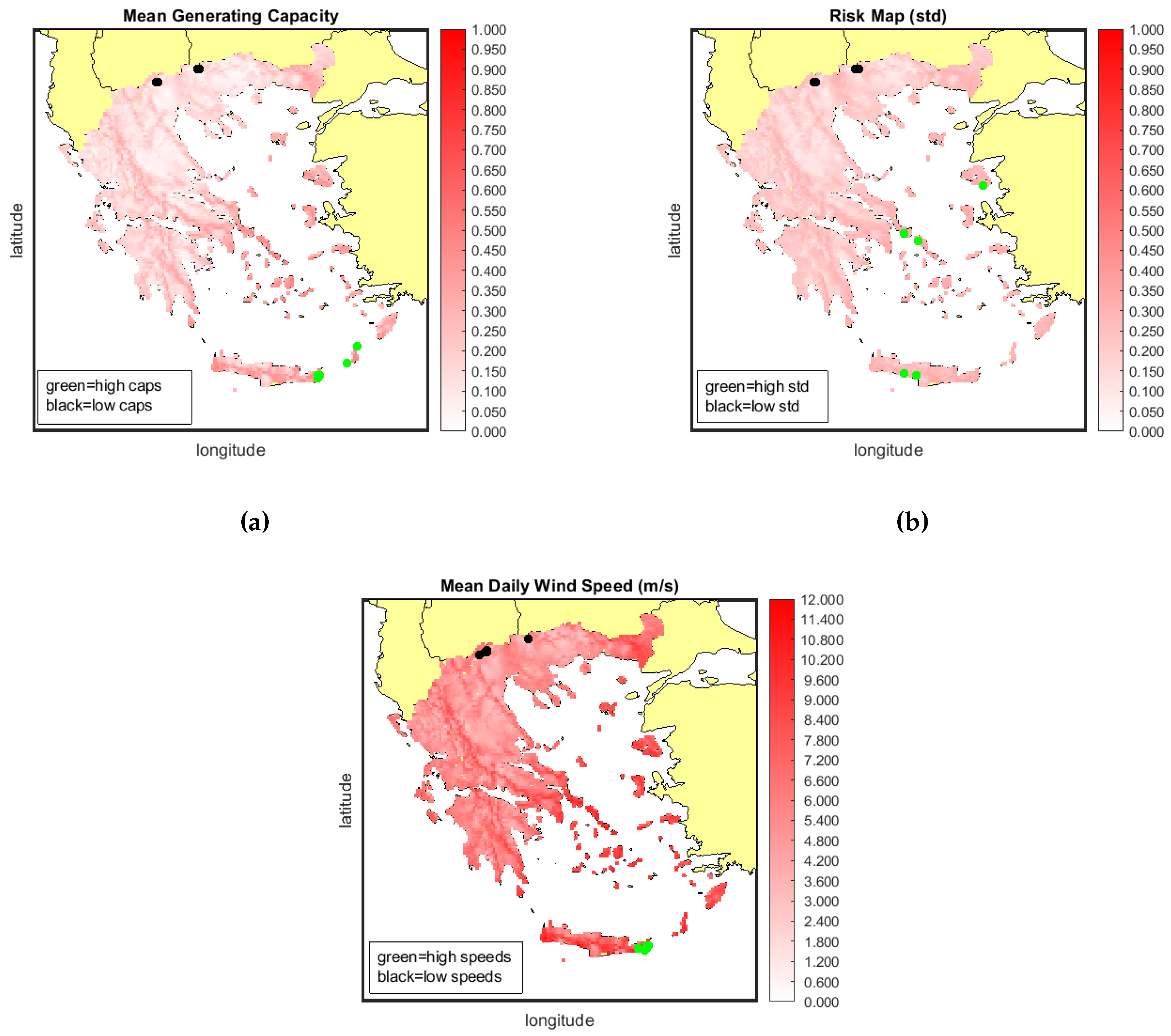
As a first step, it is important to obtain an overview of the statistical properties of our reference points. The following maps present a comprehensive wind atlas of Greece accompanied by the mean daily capacity factor and the standard deviation of each individual location with a white-to-red color gradient. Areas featuring a more intense shade of red have a higher value on the corresponding variable while the white areas are neutral (values are near zero). Locations with extremely high and low values are pin-pointed on the maps to analyze the relationship among the three variables.
Locations with rich wind profiles are mainly located over the islands of the Aegean sea and Crete. This alignment is consistent with the morphological characteristics of the Aegean Basin (wind speeds are high in sites near the sea) and the presence of the Etesian winds (Meltemia) during the summer [
46,
47,
48,
49]. Etesian outbreaks tend to have higher density in August, while they present interannual variability with a negative trend over the June to September period [
50]. Additionally, these outbreaks experience heightened occurrence over elevated terrains such as the Pindos mountain range and other lofty landscapes, where wind speeds are notably elevated. The volatility levels on
Figure 2b, are quite the same for all the grid points. However, there is a slight change in the hue that follows the same pattern with the mean generating capacity: Coastal and mountain areas have high values both in
and
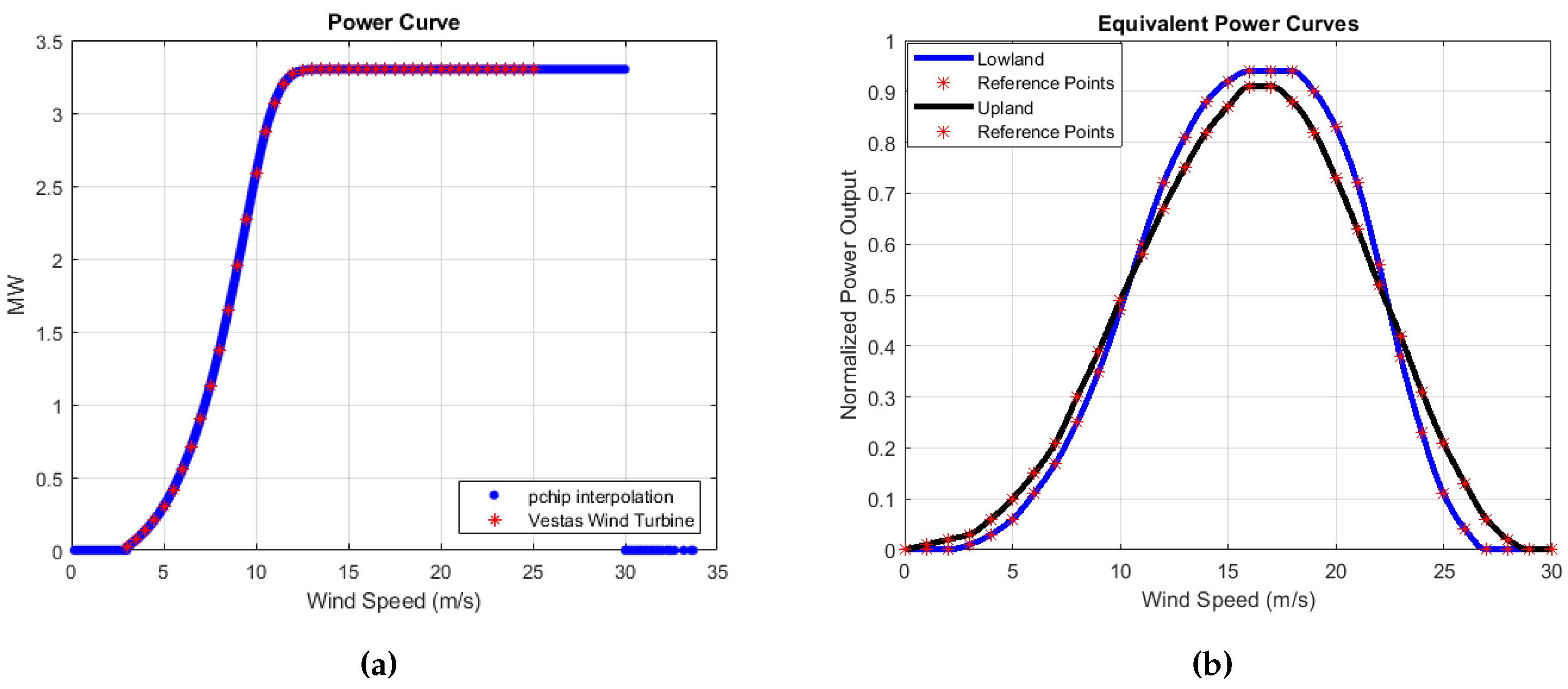
and all the other areas have lower values. It is noteworthy that the geographical locations associated with the highest and lowest wind speed values on the map are in close proximity, although not identical, to those correlated with the highest and lowest capacity factors. The EPC model incorporates specific threshold values for wind speeds on both ends of the spectrum, resulting in abrupt increases or decreases in power output. This effect is particularly pronounced in coastal sites where elevated wind speeds prevail, a phenomenon amplified by the presence of the Etesian winds (Meltemia) during the summer months. At the same time, the relationship between daily generating capacity and standard deviation is not strictly linear as the five most volatile regions differ from those with the highest generating capacity. Conversely, locations characterized by the lowest generating capacity align with those of the lowest volatility levels.
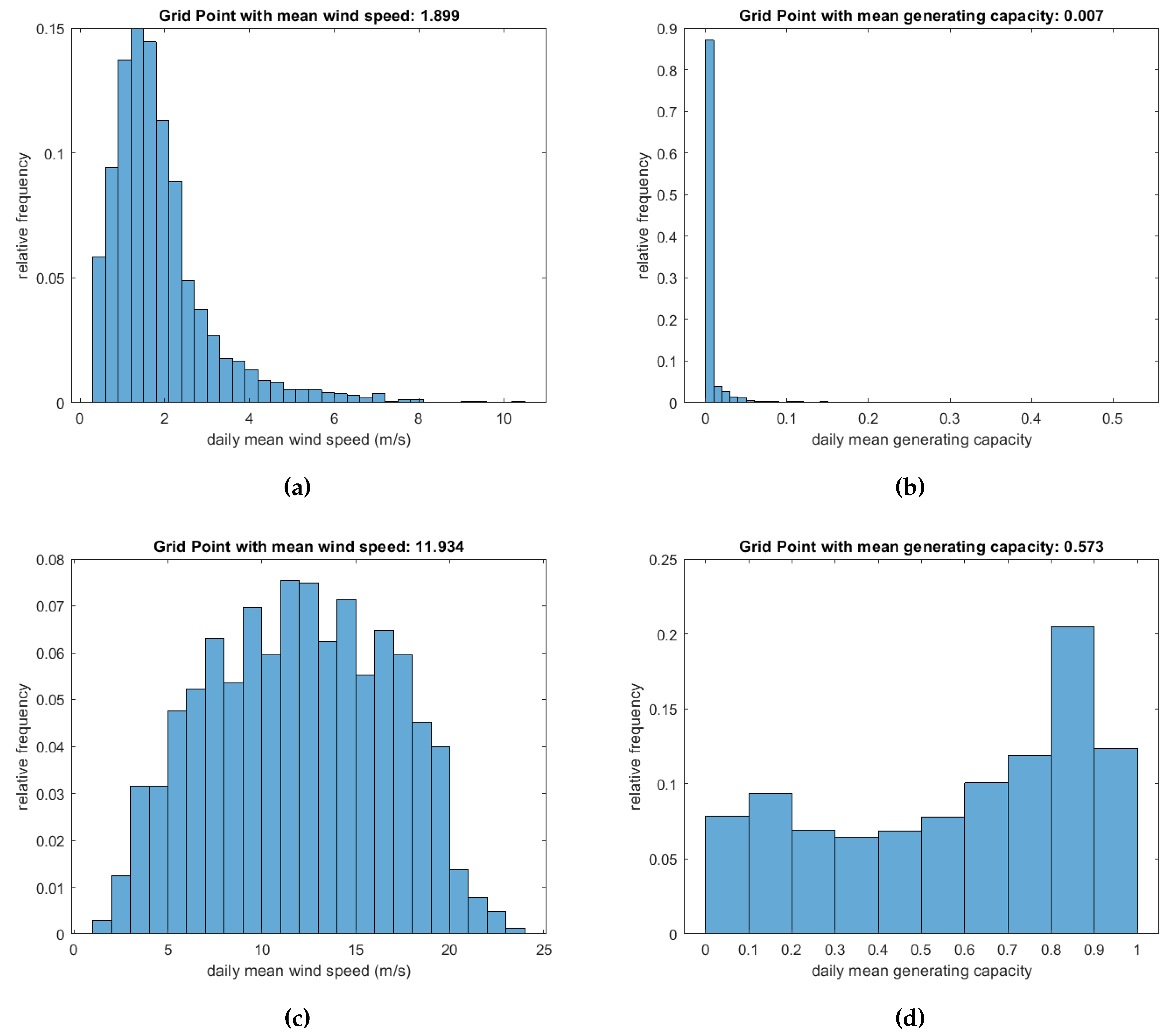
The relationship between wind speed and power output can be further investigated by drawing the distributions of the grid points featuring the highest and lowest values. An area with weak winds has a right skewed distribution, the generation profile is more stable and extreme weather phenomena are rare. On the opposite case, selecting areas with strong winds generates a distribution closer to bell-shaped curve. The generation follows a similar schema, low wind speeds produce values close to zero due to the cut-in threshold. High wind speeds on the other increase the scenarios of higher generation and the distribution is shifted on the right side.
The study of Kotroni et al. [
24] revealed a significant reliance of wind potential on the slope of the Greek terrain, rather than solely on the absolute elevation. This observation is somewhat reflected in the above-discussed maps and wind generation distributions. An other compelling aspect of wind generation is that it is positively correlated with the variability. This formulates a high risk-high reward relationship which is provided by the nature, as show on the left panel of
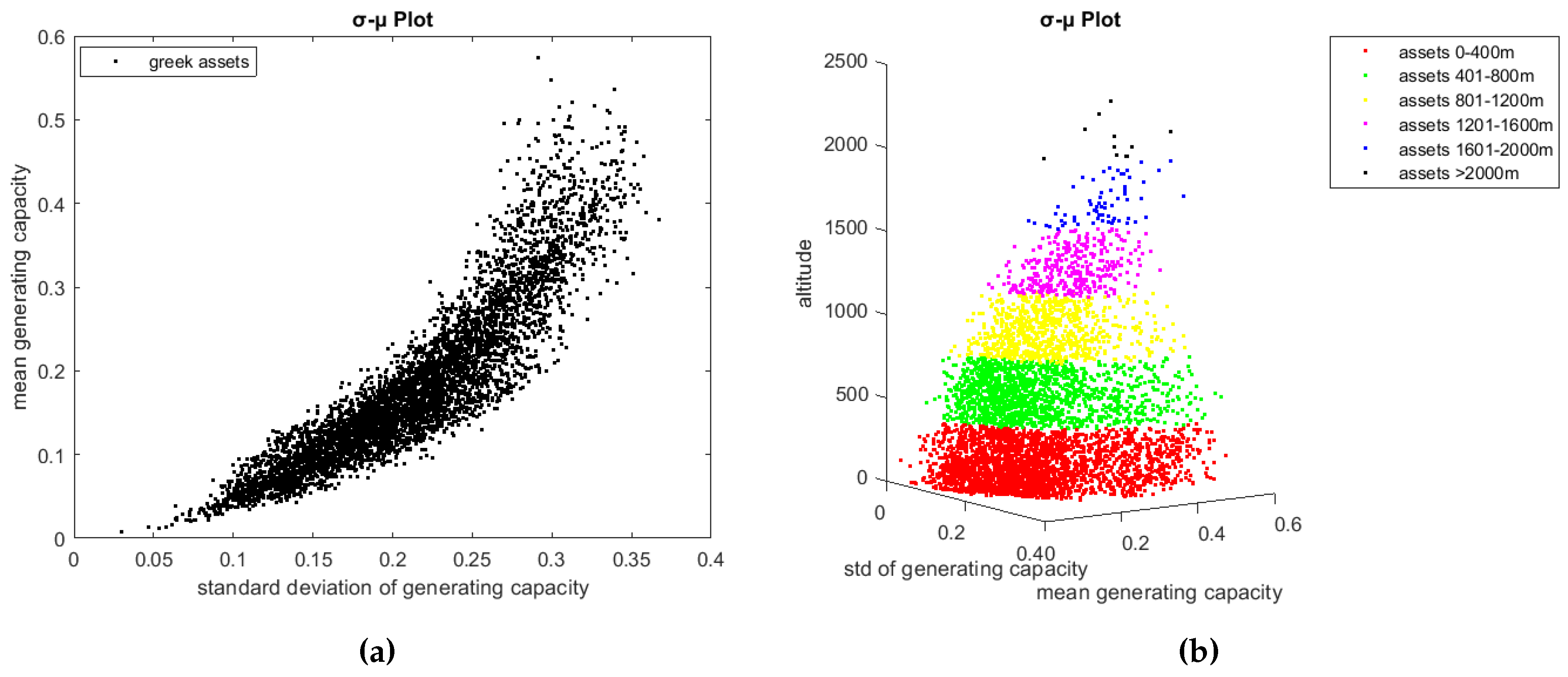
Figure 4.
Figure 3.
Histogram of highest and lowest daily mean wind speed and generation.
Figure 3.
Histogram of highest and lowest daily mean wind speed and generation.
The addition of one unit of volatility on a single asset, increases the observed mean generating capacity. This pattern mirrors a common occurrence in financial products, such as those within the stock market, where a delicate balance between risk and return is established. Individual investments will embrace extra risk only in exchange of higher generating capacity, according to the risk appetite of the investors. This is known as a "no-free-lunch property". The presence of this phenomenon within wind generation output is indeed quite noteworthy, emphasizing the potential pitfalls associated with hasty site selection. Seeking yield aggregators or other investors may lose control of risk. Selecting optimal sites is a complex endeavor, requiring a delicate balance between risk and return aligned with defined targets. The exploration of this observed relationship in natural systems holds promise for revealing valuable insights into weather variables. Moreover, it could pave the way for the inception of innovative business ventures that leverage these insights to create novel projects with sustainable returns.
In the right panel of
Figure 4, we present a visualization of 6 different classes of
points according to their altitude. Our analysis does not reveal a discernible relationship between the altitude of locations and the mean generating capacity or standard deviation within our sample. Other possible meteorological factors that could relate these variables are the logarithmic profile of the wind speed, mountain winds phenomena and the intensity of the pressure systems and fronts that cross the area of interest. A further investigation of this direction is out of the scope of this paper.
5.2. Factor Model Estimation
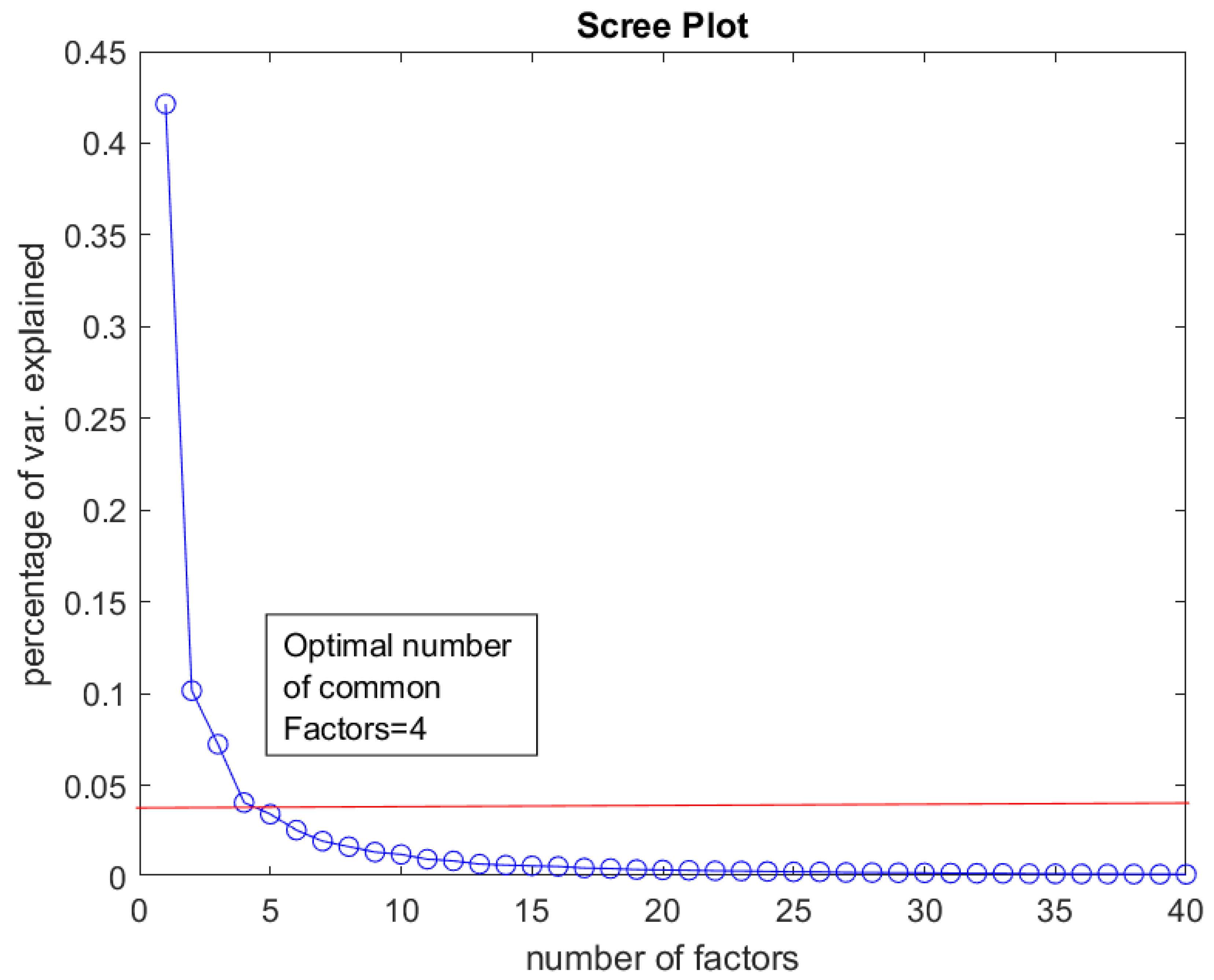
The PCA estimation of the factor model described on 4.3, shows that 4 systematic risk factors explain the 63.562% of the total variance of the panel and the rest 36.438% is explained by the non-systematic component. On
Figure 5 down below, we present the scree plot of our data. The horizontal axis shows the number of common factors and the vertical axis shows the percentage of variance that is explained by each factor. The slope is getting flat after the fourth common risk factor and this is the optimal number that should be selected. Alessi et.al criterion leads to the same result as well.
On
Table 1, it is displayed the percentage of variance explained by each common factor. The first common factor holds prominence, as it explains a significant amount of the total variance (42.13%) while the subsequent factors, in comparison, explain smaller percentages.
The conspicuous commonality observed among the grid points implies a great level of resemblance in the power generation profiles across these points, underscoring a consistent pattern. Following the estimation of principal components, a straightforward approach for gauging the exposure of each grid point to the common risk factors is through loading maps employing a blue-to-red color scale, delineating negative to positive associations.
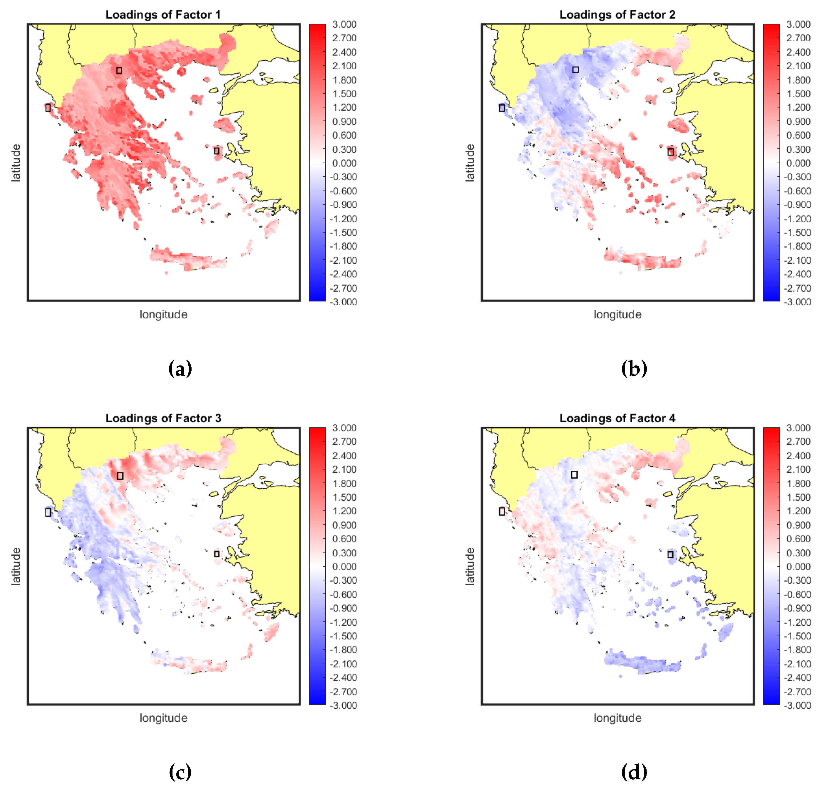
In the upper left panel of
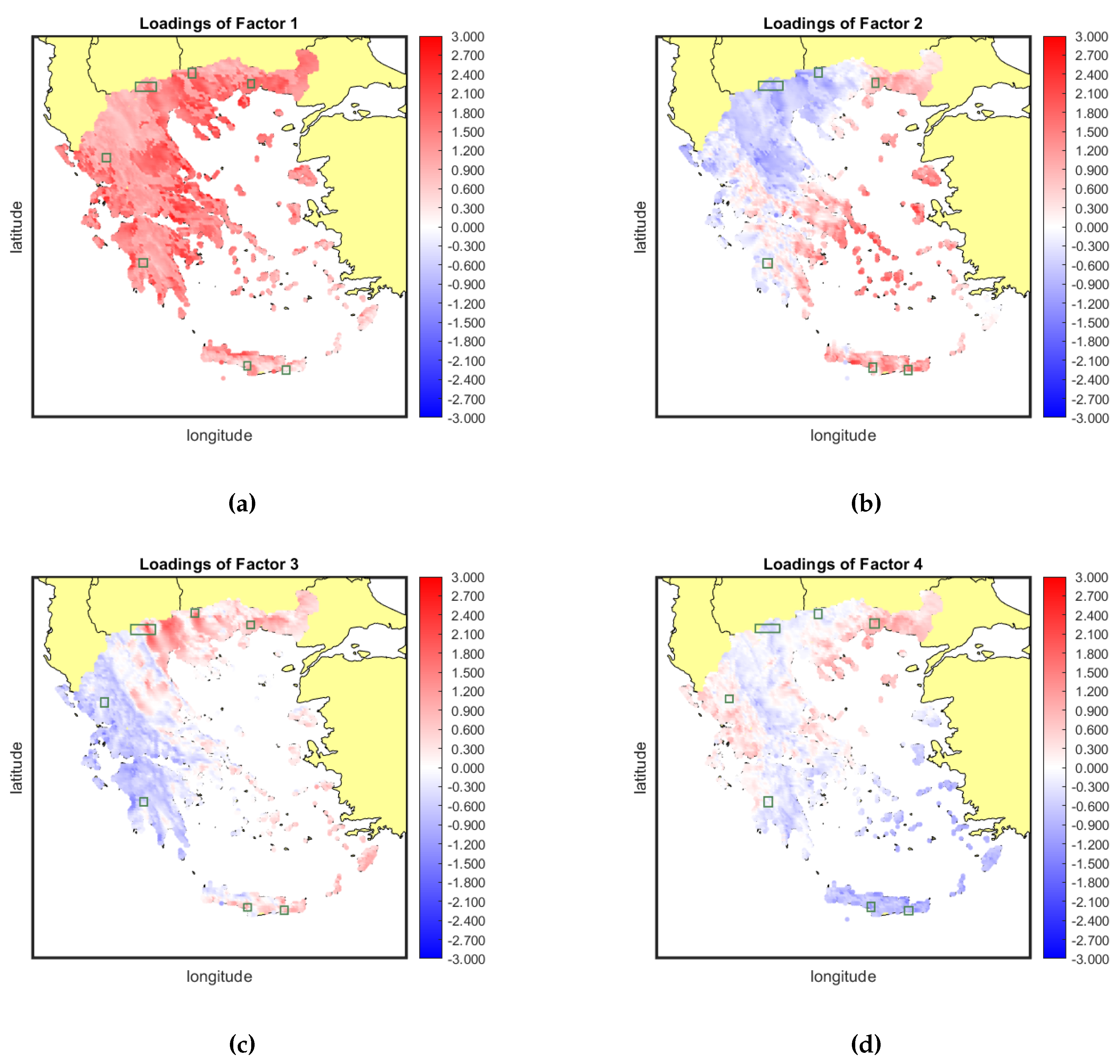
Figure 6 we depict the loadings of the 5182 sites to the first factor. Negative loadings are represented by blue hues, while positive loadings are indicated by red hues. All areas are positively exposed to the first common factor and the coastal areas have an even deeper shade of red compared to mountainous areas. This situation hampers the diversification potential of the first systematic risk component since there are no blue areas to offset the positive exposure to these specific weather conditions. Therefore, 42.13% of the uncertainty in wind generation is non-diversifiable. A simple hypothesis is that this factor explains the variability of the mean daily wind speed with respect to the elevation. As it can be seen in
Figure 6, elevated areas (such as the Pindos Mountain rigde) are clearly distinguished from the low land areas, such as in central Macedonia or Thessaly. All the other factors, are characterized by loadings of mixed sign leading to a distinctive division of the Greek territory. For factor 2 there is a blue group of provinces in north-eastern Greece and a red group of provinces in the south-western Greece. This factor can be mainly attributed to the presence of the Etesian winds which are characterized by high variability and outbreaks that extend for around a week with calmer intervals [
50]. Constructing a well-balanced portfolio involves strategically incorporating areas that demonstrate both positive and negative exposure to this particular common factor, effectively mitigating approximately 10.15% of the systematic variance. A similar phenomenon is evident for the third factor, albeit with some variations in the delineated zones. In this instance, the blue zone is primarily concentrated in the eastern and northern parts of Greece, while the red zone extends across the southern region and the Aegean Sea. This factor contributes to an additional 7.23% of variance, which potentially could be diversified. As progressing further to less eminent factors, the spatial patterns tend to become less defined, displaying a greater degree of randomization in the color distributions. The mitigation of the effects stemming from these less explanatory factors becomes less significant, with not strictly defined color zones. The elimination of the effects of that factors becomes less critical. In the best case scenario, a portfolio should incorporate areas with mixed signs in at least two or three factors.
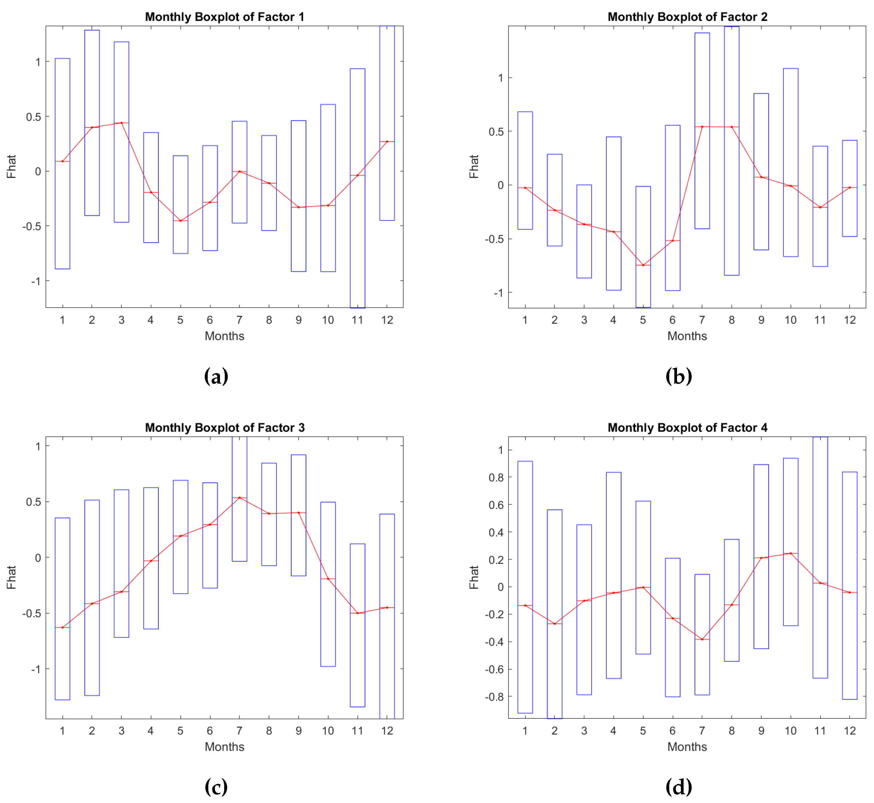
The loadings map is a static description of the exposure of the mean generation level to the systematic risk factors. To gain a comprehensive understanding of the seasonality effects on generating capacities driven by these risk factors, we construct monthly boxplots for the factor scores. Winter months typically exhibit higher mean generation levels, accompanied by elevated levels of volatility. Conversely, summer months tend to showcase the opposite trend. These patterns are likely to display variations based on the color zones indicated by the loadings. These color zones highlight distinct geographical areas with differing risk factor exposures.
The monthly averaged factor scores across all factors unveil distinctive patterns of seasonality that exert an impact on wind power generation. This seasonality not only influences the mean generating capacity but also imparts changes to the variability of this variable, evident through variations in the length of the boxes across seasons. Specifically, the generation of factor 1 tends to be higher and more volatile during winter months and at the beginning of spring, while it declines on the summer months (both for the mean production and volatility). The latter may be attributed in the general atmospheric circulation during this period, as low pressure systems are prevail over Greece, accompanied by high wind speeds. The average generation output on a monthly basis follows a cyclical pattern with 2 increasing and 2 decreasing waves. The second factor describes a different phenomenon. The mean generation experiences a reduction during winter months, while volatility decreases at the onset of spring. On summer season, there is a great pick of production, especially in June and August which is accompanied by higher levels of variability on wind generation.This factor appears to be reflective of the interannual variability associated with the Etesian winds, as previously discussed. The intricate interactions between these wind patterns and seasonal changes contribute to the observed patterns in wind power generation and its associated variability across different months. The third factor follows an ascending trend starting from January till August, reaching its peak, and then undergoes a significant reduction in mean generation. The volatility pattern resembles that of the other factors, with lower volatility observed in summer and higher volatility in winter and spring, in line with the trends previously identified. Lastly, the fourth factor lacks a pronounce or specific pattern. Its influence appears to be associated with relatively less significant weather effects, as indicated by the loading map’s random color zones. There is a minor peak observed during the autumn season, and volatility remains lower in summer but comparatively higher across all other seasons of the year. These different factor behaviors underscore the complexity of wind power generation’s dependence on multiple weather-related variables and the intricate interactions among them.
The combination of loading maps and monthly boxplots provides a comprehensive depiction of the wind power generation profile for each geographical area. The final generation output derived from the factor model results from the multiplication of loadings and factor scores, where the sign of the loading determines the overall impact of a factor on the area’s generation. For instance, focusing solely on the first factor, a reduction in generating capacity is anticipated across all areas during the summer months. This is due to their shared positive loading exposure to Factor 1. Coastal areas, characterized by higher loading coefficients, will experience a more substantial impact. Conversely, the second factor yields a distinctly different effect across the two color zones due to temporal variations. Locations with positive loading coefficients (red areas) are expected to witness increased mean daily generation during summer, whereas those with negative loading coefficients will observe decreased production during the same period. This observation underscores the benefit of including locations with mixed-sign loadings in a portfolio solution. The patterns for the third and fourth factor closely resemble each other. In areas with red (positive) loading coefficients, higher factor scores correspond to an increase in output, whereas blue (negative) areas exhibit a decrease in production with higher factor scores.
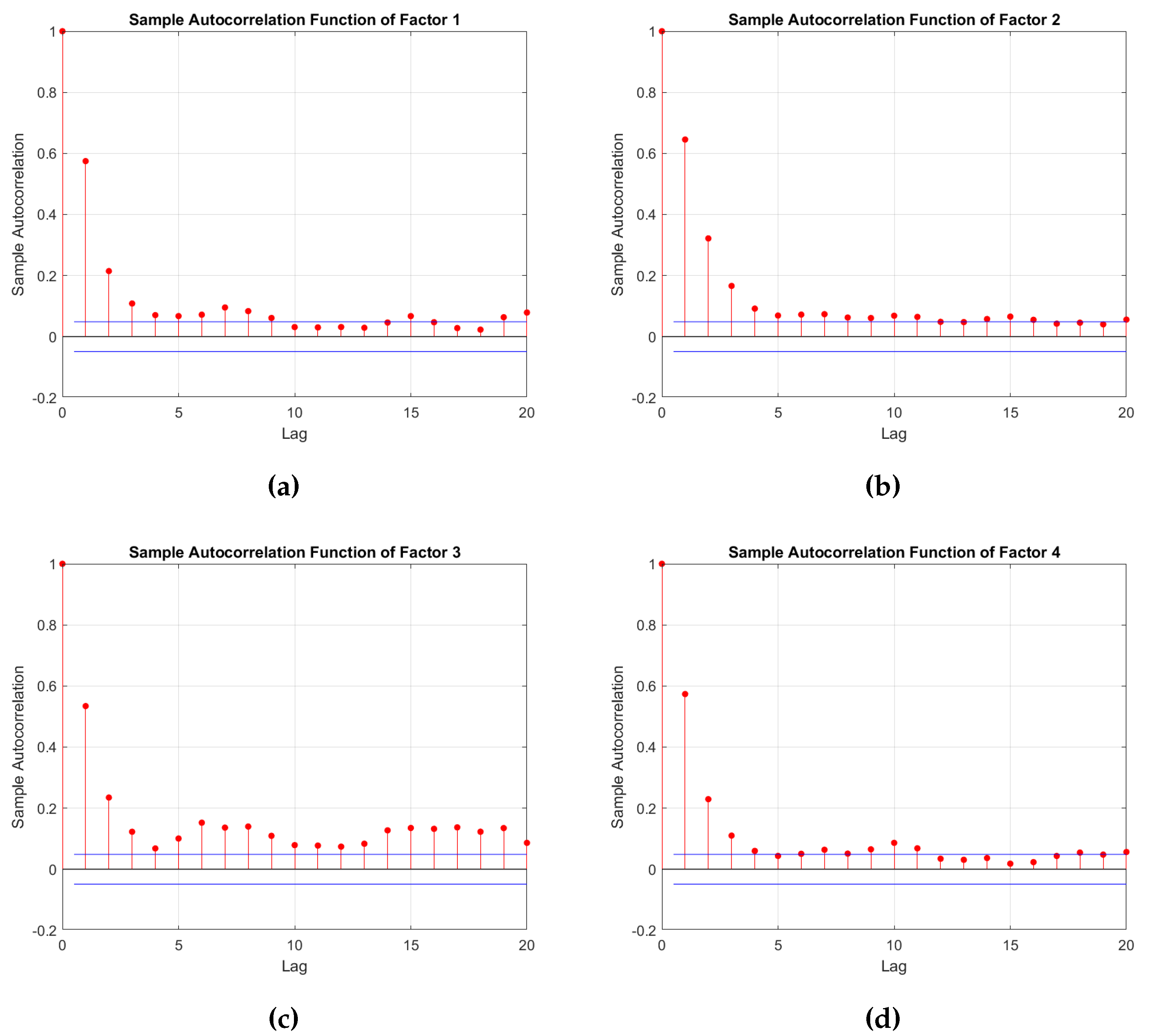
A final aspect to consider about the risk factor properties is the autocorrelation structure. The degree of autocorrelation provides insights into how a sudden disturbance in the factor scores can impact the average generation output over time. A high level of autocorrelation suggests that a disturbance in the factor scores will have a prolonged effect on the average generation output. This means that any seasonal or patterned changes will persist over an extended duration before subsiding. On the other hand, a low level or lack of autocorrelation indicates that any seasonal patterns that arise tend to fade away more quickly, with disturbances having a shorter-lived impact on the average generation output.
On the first autocorrelation function graph, we observe that nine lags fall within the statistically significant range on the 95% confidence interval. However, beyond the third lag, disturbances in the factor values gradually diminish, characterized by a subtle wave-like pattern. This suggests that the effects of the first factor are not particularly persistent, with disturbances tending to dissipate relatively quickly. Moving to the second factor, a consistent and rapid decay is observed in the autocorrelation after the fifth lag. The autocorrelation persists until the 12th lag, indicating a more prolonged influence of this factor. This implies that the effects of the second factor are more persistent compared to the first factor. Factor 3 stands out with a high level of autocorrelation and persistence. Across all 20 lags depicted on the graph, the autocorrelation values remain significantly distant from the insignificance zone. This observation signifies that factor 3 has a lasting impact on the mean generation, with its effects extending over a substantial duration. Conversely, factor 4 demonstrates weaker persistence, as indicated by the autocorrelation of only order 5. This implies that the influence of factor 4 diminishes more rapidly compared to the other factors.
5.3. PCA and Area Selection
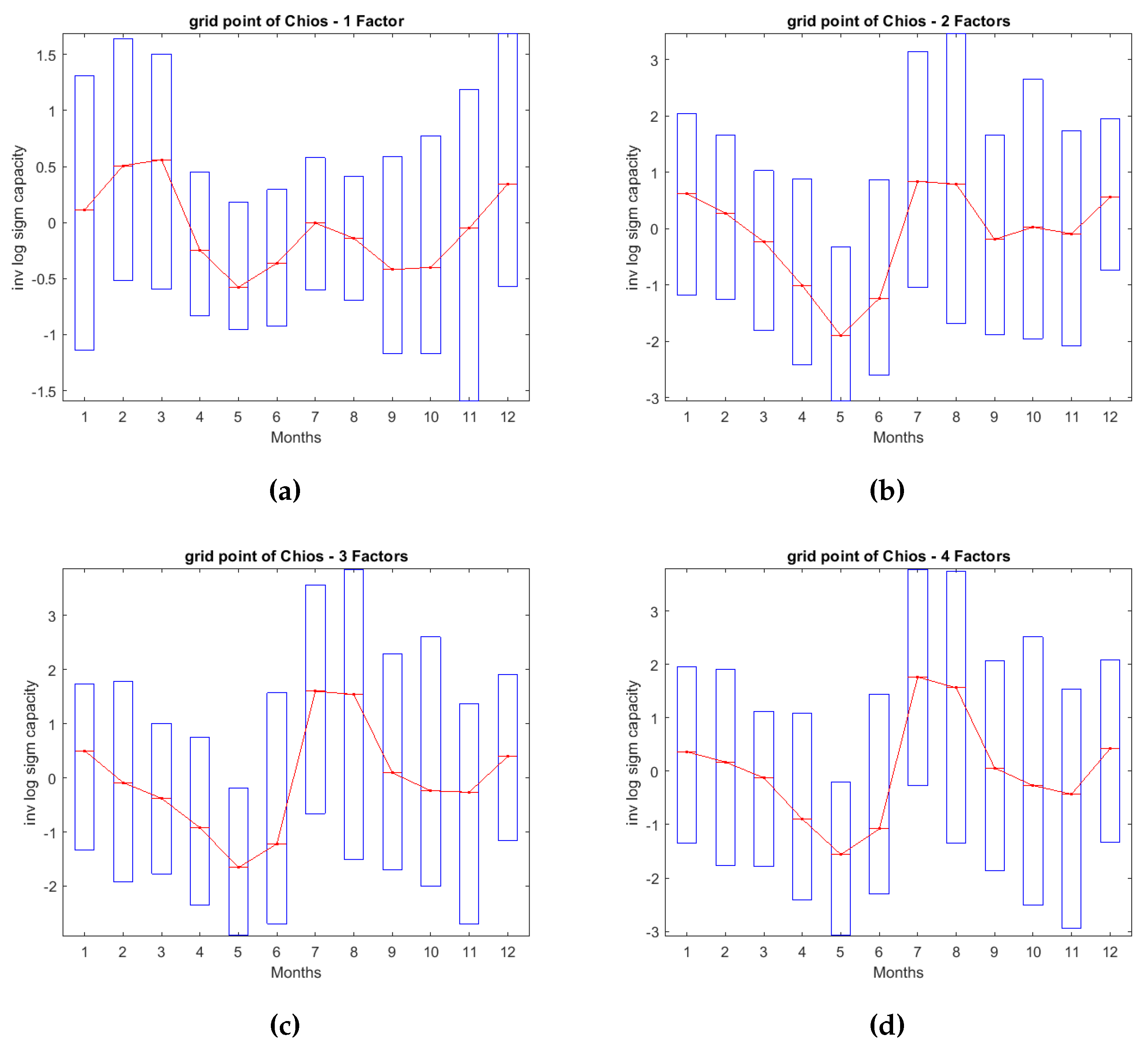
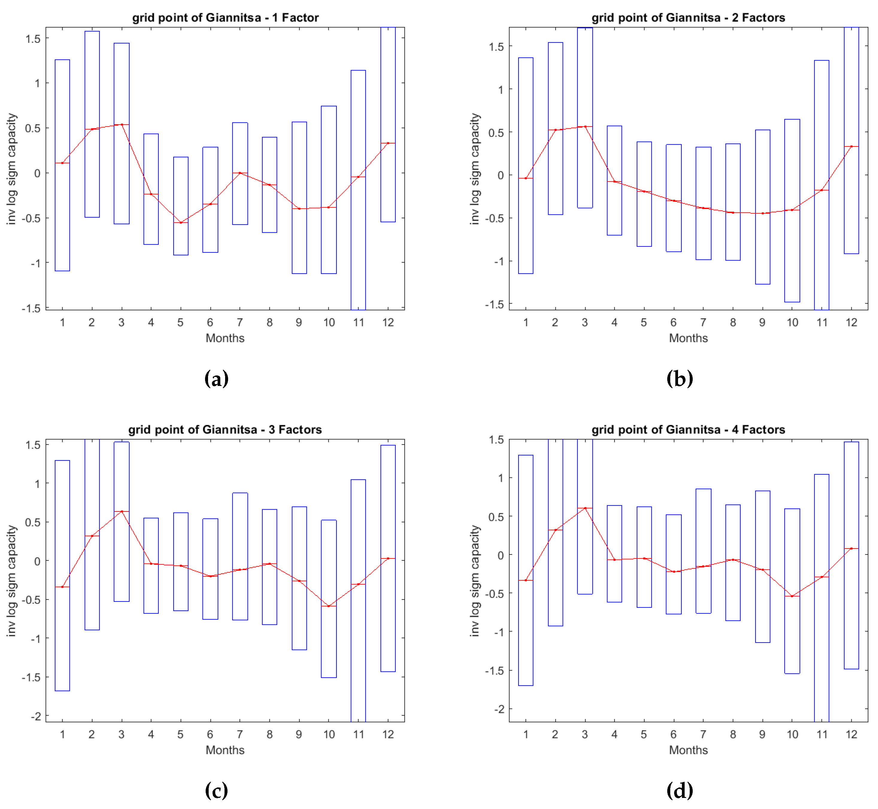
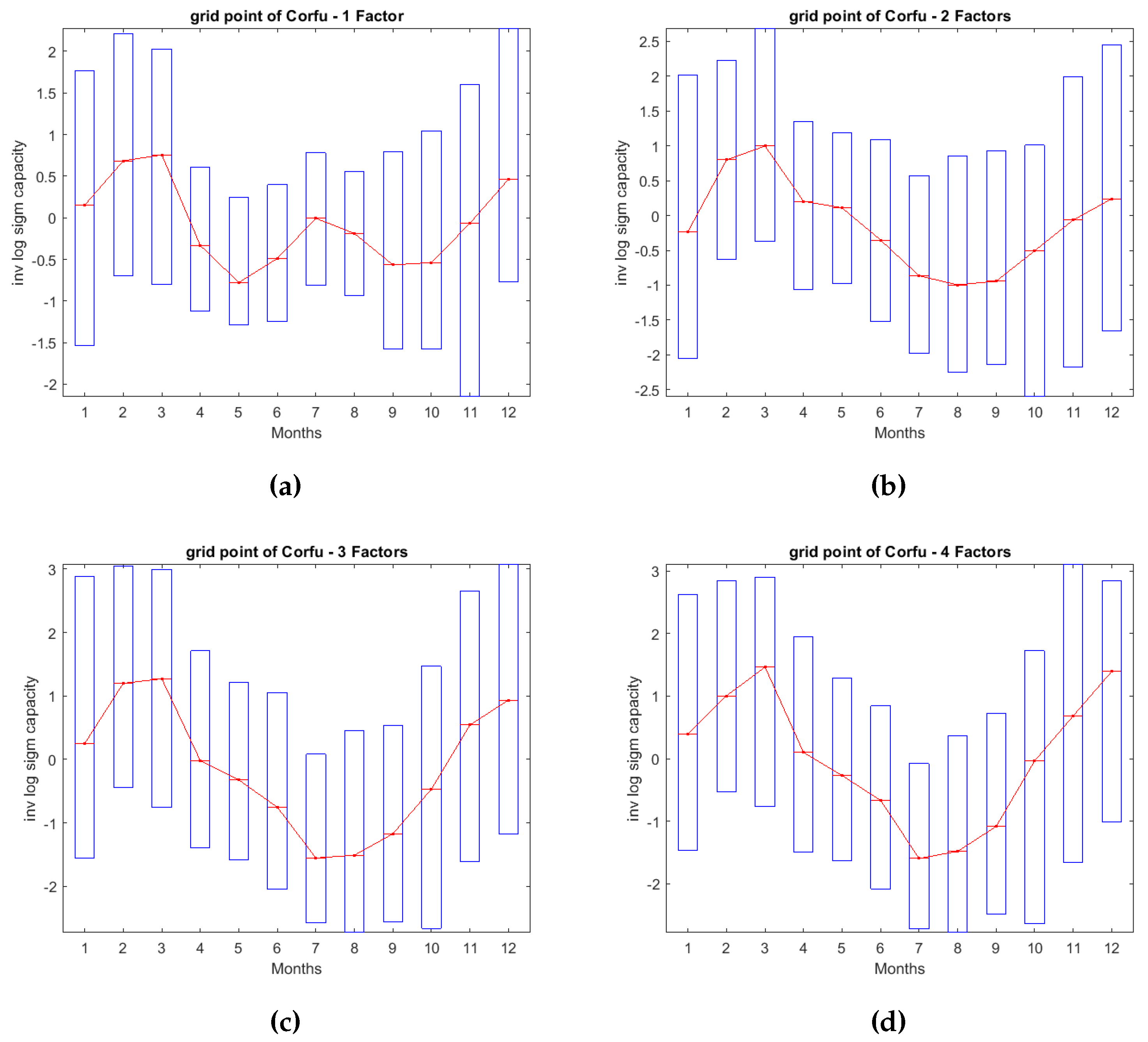
In the previous section we estimated the factor model and analyzed the fundamental properties of the common risk factors. A more in-depth comprehension of how each specific factor uniquely contributes to the model can be achieved through the reconstruct analysis framework. The gradual incorporation of each factor, results in an immediate transformation of the generation schema over time, thereby providing additional insights into the origins of each risk component. Given the extensive sample size, we only select 3 areas based on their loadings pattern. This selection was made to ensure that all possible combinations of exposure to the risk factors could be depicted accurately. In the following maps, the black boxes represent the 3 selected sites for the reconstruct analysis. On the first factor, only a positive sign is available, but on the second and third we can distinguish three cases: 1) Positive and positive exposure, 2) Positive and negative exposure and 3) Negative and negative exposure. The fourth factor, being of lesser significance, was not considered in the sign selection methodology outlined above, for simplicity. The chosen sites for the analysis are Chios (38.5, 25.9), Giannitsa (40.8,22.4) and Corfu (39.75,19.75). Chios has a strong positive exposure on the second factor and a weak positive exposure on the thrid factor. Giannitsa, on the other hand, demonstrate a medium negative exposure to the second factor and a medium positive exposure to the third factor. Lastly, Corfu has a moderate negative exposure to both second and third factor. The monthly averaged transformed generation of these 3 assets is anticipated to be different as each factor is added. To validate this statement, we created the monthly averaged transformed generation capacities boxplots of the designated areas. Each factor can be conceived as a building block that is added on the overall generation schema.
For the grid point of Chios, employing only one factor gives similar results with those of
Figure 7. Upon introducing the second factor into the model, there is a noticeable decline in generation output during the winter and spring seasons, coupled with a peak in generation during July and August. This observation suggests that the Etesian winds (as mentioned in [
50]) exert significant influence during this period, leading to a positive impact on the area’s generation output. The third factor does not add any significant alterations to the generation pattern except some minor declines on the winter months. The fourth factor enhances the production a little bit on July but it does not change the production output to a remarkable level. The grid point of Giannitsa is characterized by a different generation profile. The first factor affects the transformed capacities in a manner similar to that of all the other grid points (higher generation within winter and early spring months). When the second estimated factor is incorporated on the model, the averaged monthly transformed generation undergoes a steady reduction during spring and summer, without the production picks seen in Chios. This decrease is accompanied by low levels of volatility. The third factor contributes to greater stability in the transformed capacities by slightly increasing production during spring and summer, a phenomenon potentially explained by the positive loadings on this factor. The fourth factor does not add any considerable points. Lastly, for the grid point of Corfu, we observe the same pattern for factor 1 alike to the other areas. The addition of the second factor, imposes a decline on the transformed capacities for spring and summer accompanied by increased volatility indicated by the length of the boxes. The latter shows the variability of the wind speeds during these months, since both synoptic (e.g. front passages) and thermodynamic conditions (e.g. thunderstorms) affect the wind field. The third factor amplifies the impact of the second factor, leading to a further decline in average production. As for the fourth factor, it only generates a minor peak in average production during March, with no substantial alteration to the overall generation pattern.
Figure 7.
Monthly boxplots of the 4 principal components.
Figure 7.
Monthly boxplots of the 4 principal components.
Figure 8.
Autocorrelation function of each one of the systematic risk factors.
Figure 8.
Autocorrelation function of each one of the systematic risk factors.
Figure 9.
Factor Loadings on designated areas.
Figure 9.
Factor Loadings on designated areas.
Figure 10.
Monthly averaged transformed generation of Chios.
Figure 10.
Monthly averaged transformed generation of Chios.
Figure 11.
Monthly averaged transformed generation of Giannitsa.
Figure 11.
Monthly averaged transformed generation of Giannitsa.
Figure 12.
Monthly averaged transformed generation of Corfu.
Figure 12.
Monthly averaged transformed generation of Corfu.
5.4. Minimum Variance Portfolio
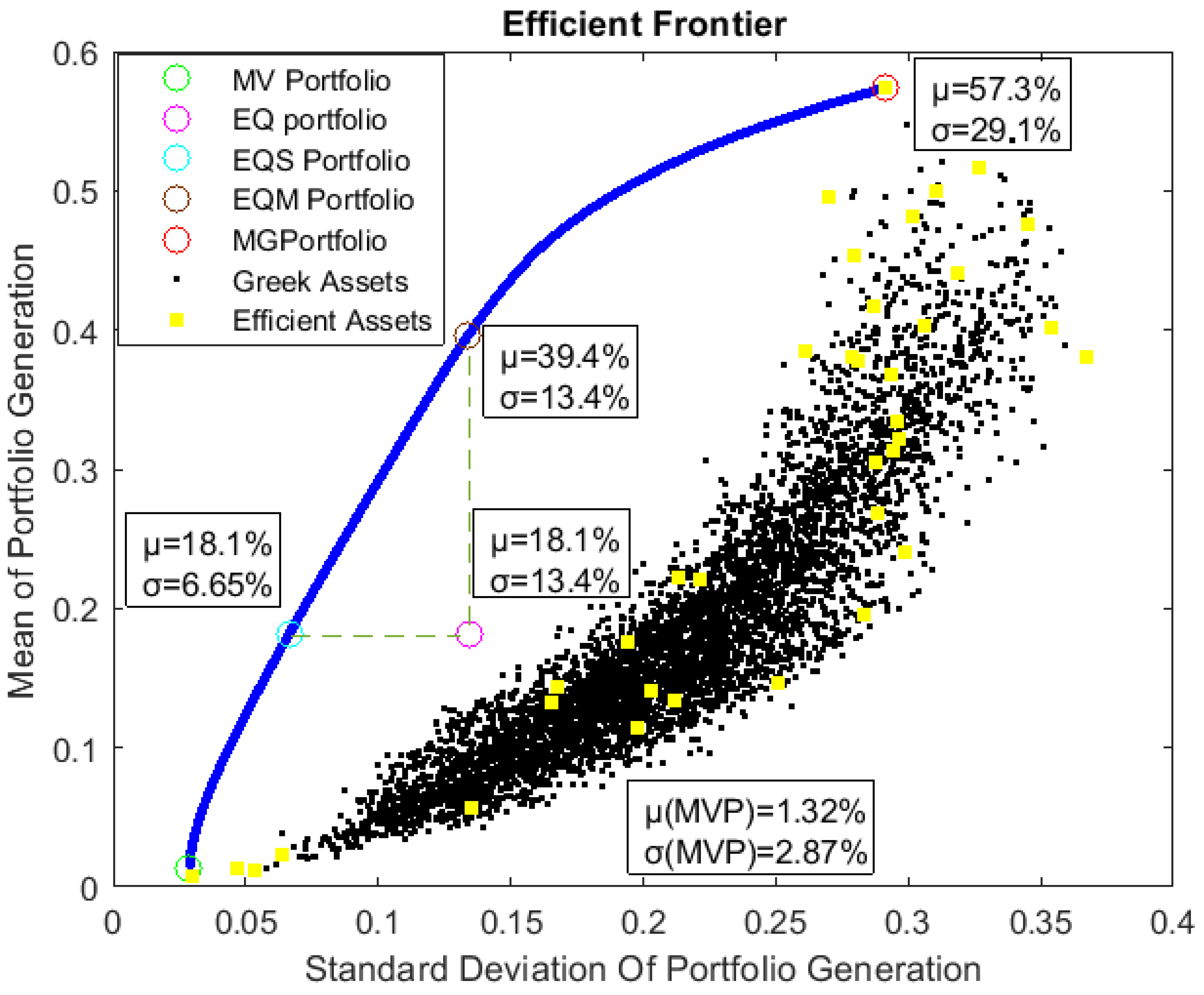
The quadratic optimization problem was structured in accordance with the framework presented in Section 4.2. It contains an asset universe of and it was solved for 50 portfolios to construct the efficient frontier, starting from the MVP until tne Maximum Generation portfolio (MG). The Equally Weighted Portfolio (EQ) and the Efficient Equally Weighted Portfolios (EQS,EQM) were also distinguished for assessment as alternative solutions in place of the MVP. Furthermore, on each efficient portfolio, we decided to focus only on the locations that have a considerable share of allocated capacity (greater than 0.1%). This criteria led to a total of 35 efficient assets with only a subset of these areas being included in each portfolio. This is a promising outcome for a practical implementation of a wind farm installation project as the cost-benefit ratio will be greatly improved in comparison with a simplistic site selection technique. In addition, any environmental concerns and other barriers for installing too many wind turbines across one or more areas can be overcome upon the claim of the cardinality of the optimal spatial allocation plan.
Figure 13 presents the
pairs of each individual asset and of the 50 efficient portfolios. The MVP solution contains only 9 areas (each one with a weight
) and has a mean generating capacity of
and
.
This solution instantly highlights one of the shortcomings of the MVP approach: The seek of a portfolio with the lowest levels of volatility often leads to a significant reduction in mean generating capacity as well. This calls into question the practicality of implementing such an allocation plan. However, in cases of an efficient frontier with a steep slope, alternative portfolio solutions can increase the mean generating capacity to a great extent by accepting only a small increase in the portfolio volatility as well. For instance, the EQS Portfolio, has an which is much higher than the MVP mean generation but the standard deviation is higher only by approximately 4%. It is worth noting, however, that instead of solely relying on and statistics, various other criteria will be considered later in the decision-making process for the final portfolio. These include Principal Component Analysis (PCA), exposure to systematic risk factors, distribution characteristics, and the frequency of near-zero production, among others.
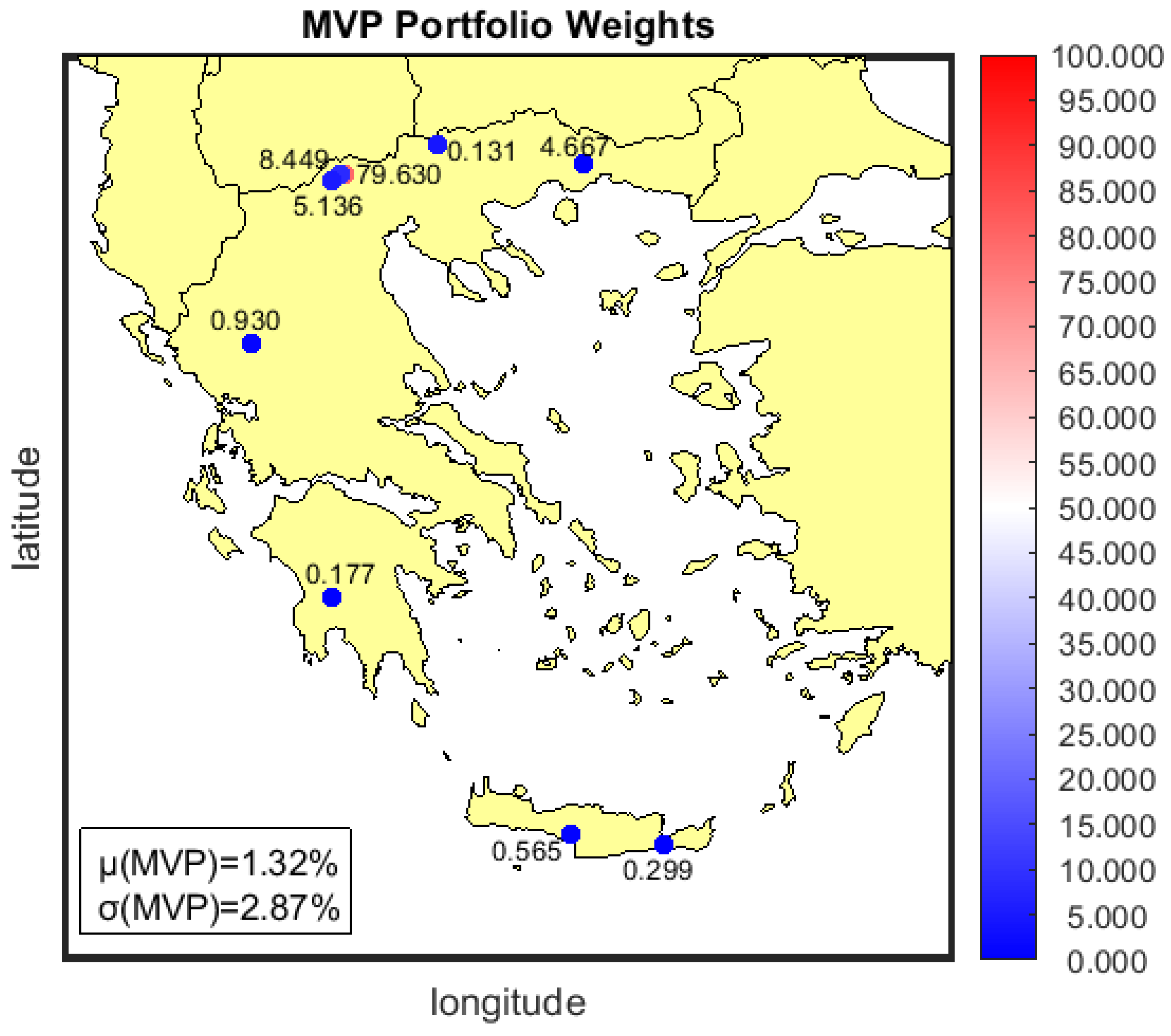
The MVP solution is graphically represented in
Figure 14. There are three assets on municipality of Almopia (prefecture of Pella) and one of them is the dominant asset of the portfolio by absorbing the 79.63% of the total installed capacity. The other 2 assets absorb approximately 13% of the total installed capacity (8.44% and 4.66%). Tzoumerka mountains (prefecture of Ioannina) have a capacity share of 5.13%. The remaining 2.2% is distributed on Peloponnese (Tsakonas), on Central Macedonia (Kerkini’s lake, near Serres), on Thrace (Xanthi) and on Crete (Agia Paraskevi, prefecture of Rethymno and Ierapetra, prefecture of Lassithi). Most of the locations of the MVP solution are on mountain terrains while 2 of them are closer to coastal areas.
5.5. Portfolio Evaluation
One method for assessing the effectiveness of diversification is to compute the Risk Reduction Index, as outlined in [
7]), which can be defined as follows:
In (11),
denotes the portfolio standard deviation and
denotes the daily standard deviation of each individual asset.
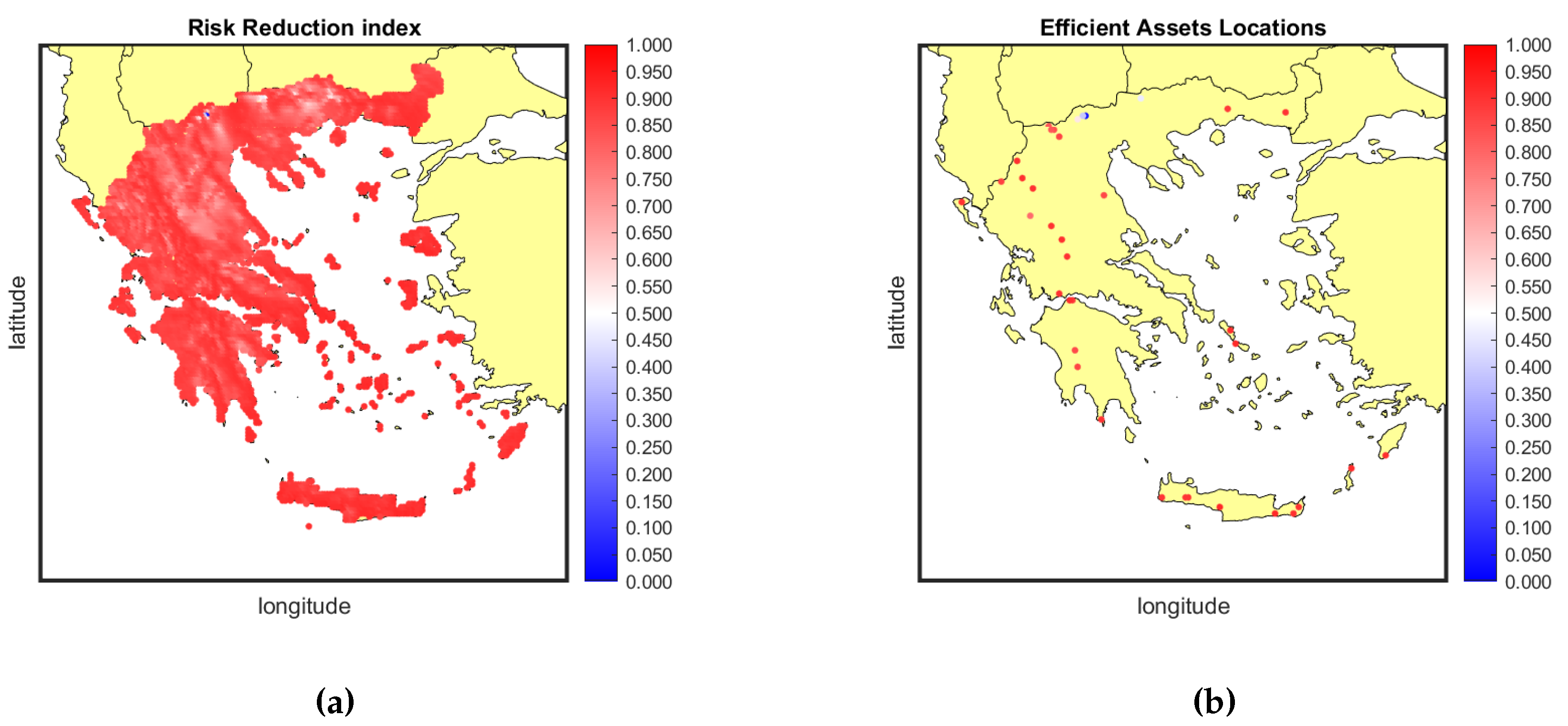
In the left map of
Figure 15a, the RR of each grid point is depicted. Nearly all areas have shades of red, indicating that inclusion in a portfolio is highly advantageous as it significantly reduces their risk. In the other map, we exclusively display the RR of each location of the efficient assets. Only 2 points have a blue color and 1 has a white color. These particular locations were chosen by the algorithm in the MVP solution due to their low variability in terms of risk.
An intriguing observation is that the efficient assets are distributed throughout Greece, spanning both mountainous and coastal regions across the country. Many grid points are situated within the mountain range of Pindos while others are found on the island of Crete. In particular, the eastern and southern regions of Crete are more suitable due to the complex terrain of the island which results in gap winds and wind flow acceleration as documented in [
24,
51]. Each of the efficient assets possesses a unique wind profile ideal for wind farm installations. For instance, in the summer season, coastal areas tend to experience higher wind speeds, while in the winter, wind speeds are elevated in the mountainous regions. This explains why both types of areas are selected by the efficient portfolios.
In addition to the Minimum Variance Portfolio (MVP) solution discussed earlier, there are other criteria that warrant consideration before finalizing the optimal allocation plan. An essential aspect to analyze is the risk exposure of the MVP portfolio to common risk factors. While diversification aims to reduce the idiosyncratic risk component by selecting areas with different generation profiles, it is possible that systematic factors may still introduce instability into the portfolio’s generation. To address this concern, we can visualize the MVP solution on a loadings map. If the locations designated by the portfolio exhibit risk factor loadings that are numerically close to zero or loadings with mixed signs, this indicates that these factors can indeed be diversified through the spatial allocation of wind generation.
In the following maps, the green-colored boxes represent the 9 MVP locations, as presented in Section 5.4. It is evident that the first risk factor cannot be diversified as all loadings are of the same sign (positive). However, the portfolio has chosen areas that, while not completely eliminating exposure to this risk component, have loadings that are not extremely high (deep red). The portfolio attempts to minimize the impact of this risk component. On the second factor, we notice that the MV portfolio areas have loadings both in the red and blue zone with the hue to varying slightly but generally not being very pronounced. This a favorable result as the portfolio can reduce or even neutralize the effect of this specific risk component by selecting areas with opposite loadings sign. The same phenomenon is also present for the third factor as 6 areas are located in the red zone while the rest are located in the blue zone with a very light hue. This factor can be as well diversified away. Finally, the last factor is diversifiable as well, given that the portfolio-designated areas feature mixed exposures to this risk component, indicated by the varied loadings.
Figure 16.
Factor Loadings on designated areas.
Figure 16.
Factor Loadings on designated areas.
To summarize these results, there is a 42.13% of total variance of the transformed generating capacities (as later shown in section 4.3) that cannot be diversified while the rest 36.438% is, to some extent, diversifiable.
5.6. Efficient Portfolios
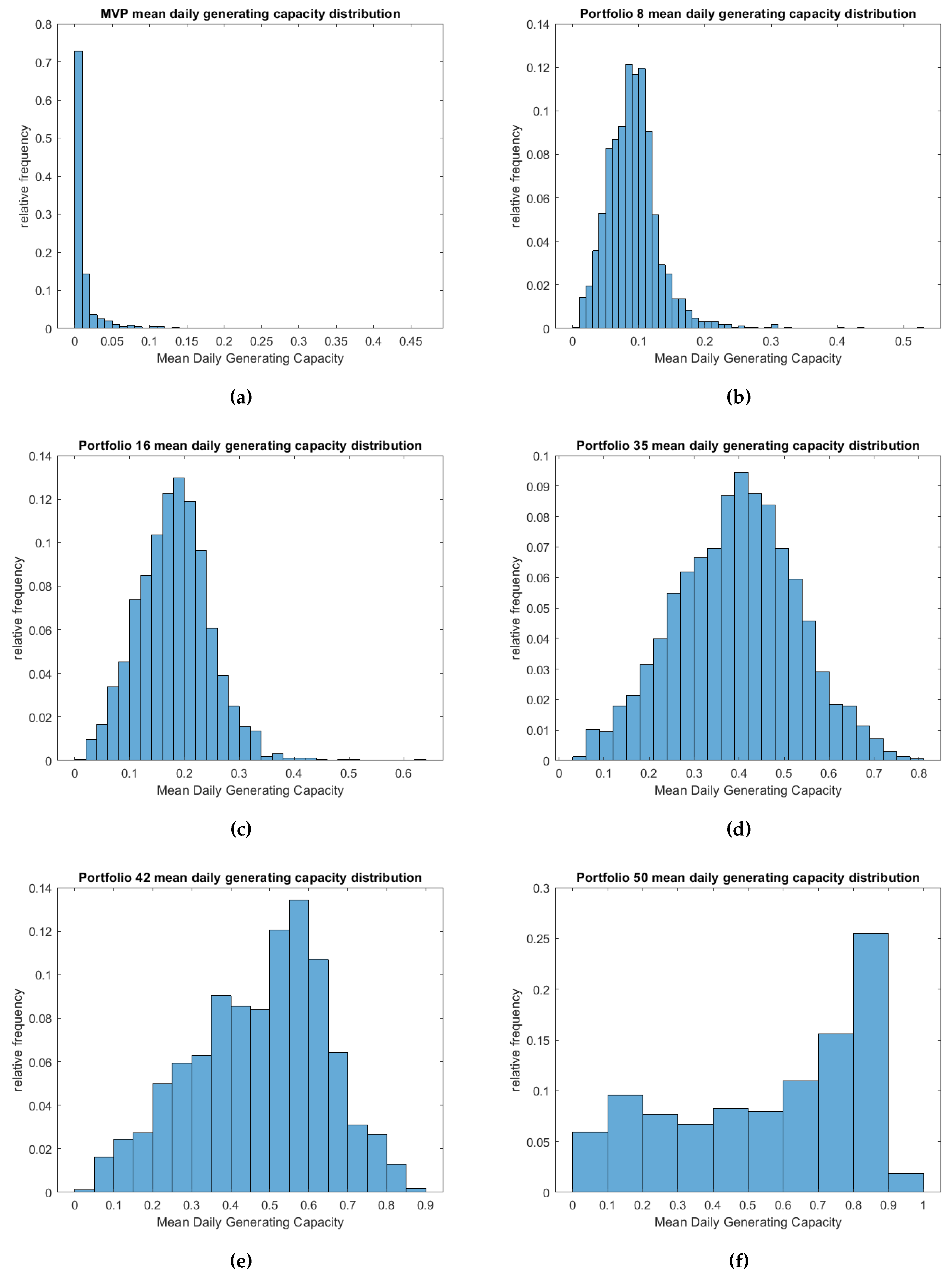
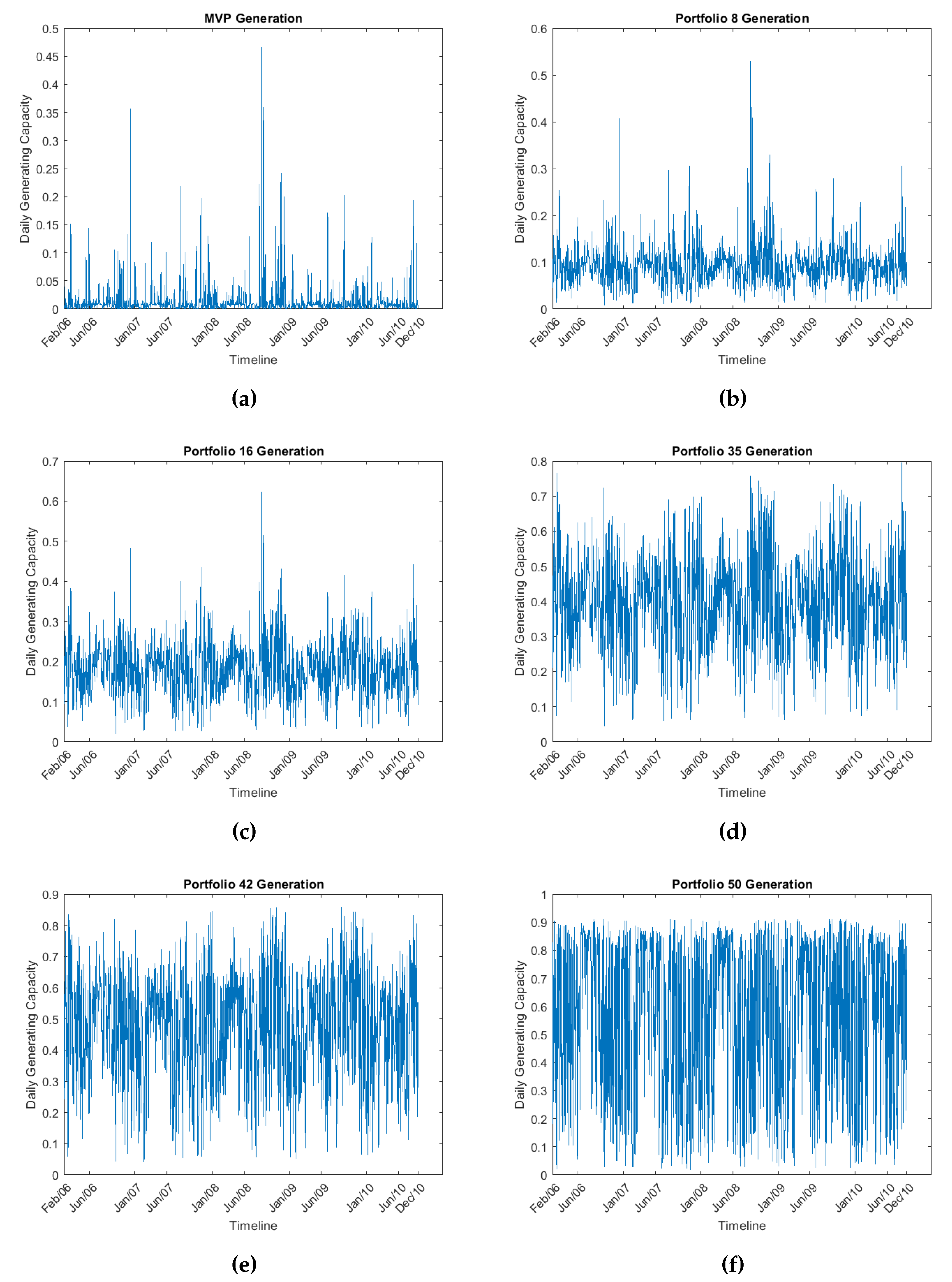
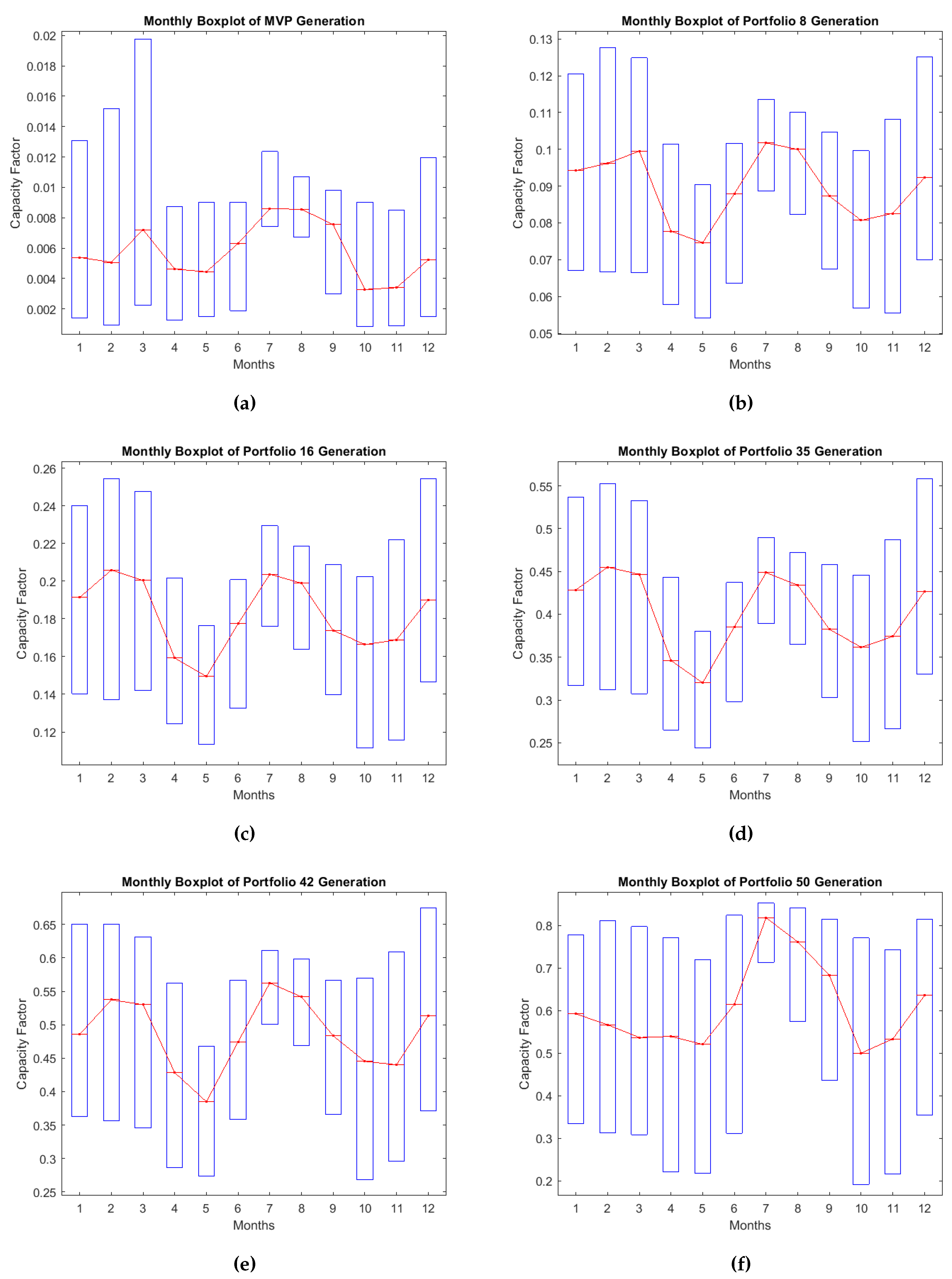
The MVP solution has been found to yield a suboptimal generation output, making it impractical for implementation in a real-world scenario. Nevertheless, given the steepness of the efficient frontier, alternative portfolios warrant consideration in determining the final spatial allocation plan. To assess these alternatives, we have generated timeplots, monthly boxplots, and daily generation capacity distributions for six random portfolios located on the efficient frontier, including the MVP, EQS and MG.
Figure 17.
Histogram of mean daily generating capacities of 6 portfolios of the efficient frontier.
Figure 17.
Histogram of mean daily generating capacities of 6 portfolios of the efficient frontier.
The histograms of relative frequencies reveal an interesting trend along the efficient frontier. In the first 20-30 portfolios a right kurtosis is observable in the distribution, particularly pronounced in the MVP. In contrast, in the final 5 portfolios, there is some degree of left kurtosis, especially in the MG portfolio. As we progress towards the middle of the efficient frontier curve, specifically in portfolios within the range of 30-40, the distribution of daily capacities gradually tends to approximate a Gaussian distribution. This phenomenon can be attributed to the inherent objectives of the optimization algorithm. To attain a significantly low level of risk, the algorithm efficiently selects locations where extreme weather conditions or very high wind speeds are infrequent. However, when the goal is to boost generation output, the algorithm must include areas with more diverse and robust wind profiles, even if this leads to increased variability.
The implementation of the MVP solution may lead to a high number of zero production days, rendering the wind farms unproductive. On the other hand, Portfolio 50 (MG) is not a viable option due to its high variability and uncertain generation output. Portfolios within the range of 16-35 present a more acceptable compromise, as they help mitigate excessive variability while increasing wind energy production. To make a well-informed decision, it’s advisable to examine these portfolios in detail, taking into account factors such as the number of selected assets, ease of wind farm installation, alignment with the surrounding environment, and micro-climate conditions. By considering these aspects, an investor can identify the portfolio that offers the best balance between risk and generation output while being conducive to practical implementation.
Figure 18.
Mean daily generating capacity of 6 portfolios of the efficient frontier.
Figure 18.
Mean daily generating capacity of 6 portfolios of the efficient frontier.
The mean daily generation of the portfolio can be computed by utilizing the optimal portfolio weights obtained from the algorithm in previous step. As we examine the time plots, it becomes clear that both the mean and variance of generating capacity have significant variations along the efficient frontier. For instance, the MVP portfolio displays multiple clusters of near-zero production days, resulting in a lower risk level. Conversely, portfolio 50 demonstrates the opposite trend with higher generation but also greater risk.
Wind speeds and other climatology variables are highly affected from seasonality. To capture the seasonal patterns in the mean daily generation of the portfolios, monthly boxplots are utilized. These boxplots reveal that mean daily generation tends to peak during the summer season for all portfolios, with an increasing trend from the MVP to the MG solution. Conversely, the winter season also experiences high wind speeds, while in spring and autumn, production decreases. This sequential pattern reflects the four seasons’ influence on generation. Moreover, the variability in production differs across seasons. Winter, marked by extreme weather conditions, exhibits significantly higher wind speed variability. In contrast, during the summer, the range of the boxes is narrower, indicating lower variability. An intriguing finding is that even in the MVP boxplot, a notable amount of variability remains, underscoring that generation risk is not entirely eliminated. In the subsequent section, factor analysis will be conducted to delve into the sources of variability in the efficient portfolios, dissect wind generation risk, and validate the results of the optimization algorithm.
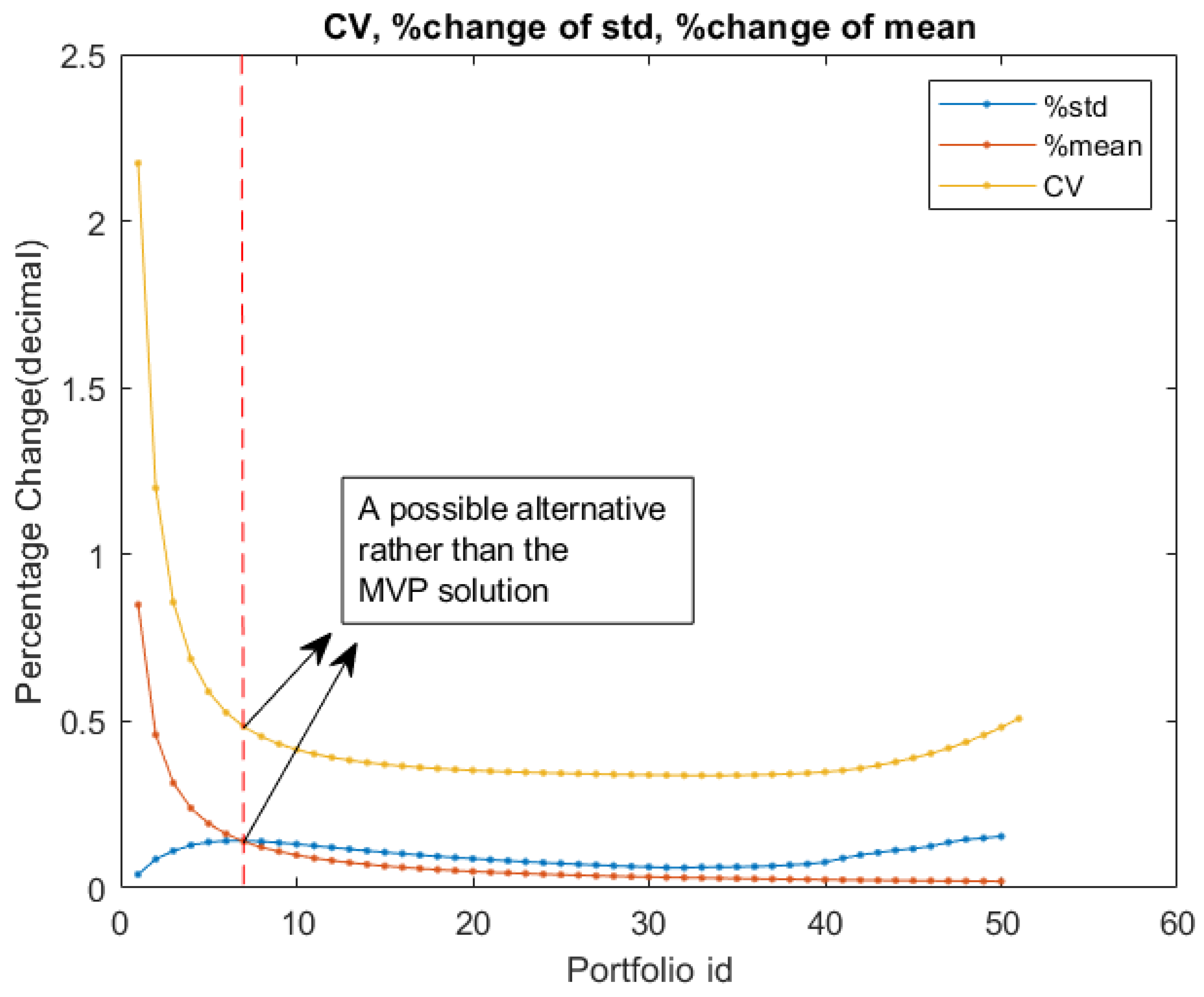
An alternative approach that can be easily applied to facilitate the selection of the final spatial allocation plan is to quantify the incremental risk, denoted as and the supplemented generation output, denoted as that is added in the sequence of the efficient portfolios along the frontier. In addition, the Coefficient of Variation (CV) can be calculated to identify the relationship between generation output and volumetric risk for each portfolio. Typically expressed as a percentage, the CV can be integrated into the same graph alongside the other two measures. This standardized relative risk measure enables a direct comparison of relative variability among different datasets, further aiding the decision-making process. If the Coefficient of Variation (CV) for an individual portfolio surpasses 100%, it signifies that the standard deviation () exceeds the mean (), indicating an unfavorable scenario. The lower the CV, the more favorable the relationship between and becomes. In fact, the optimization algorithm could be adjusted to target the minimum CV ratio.
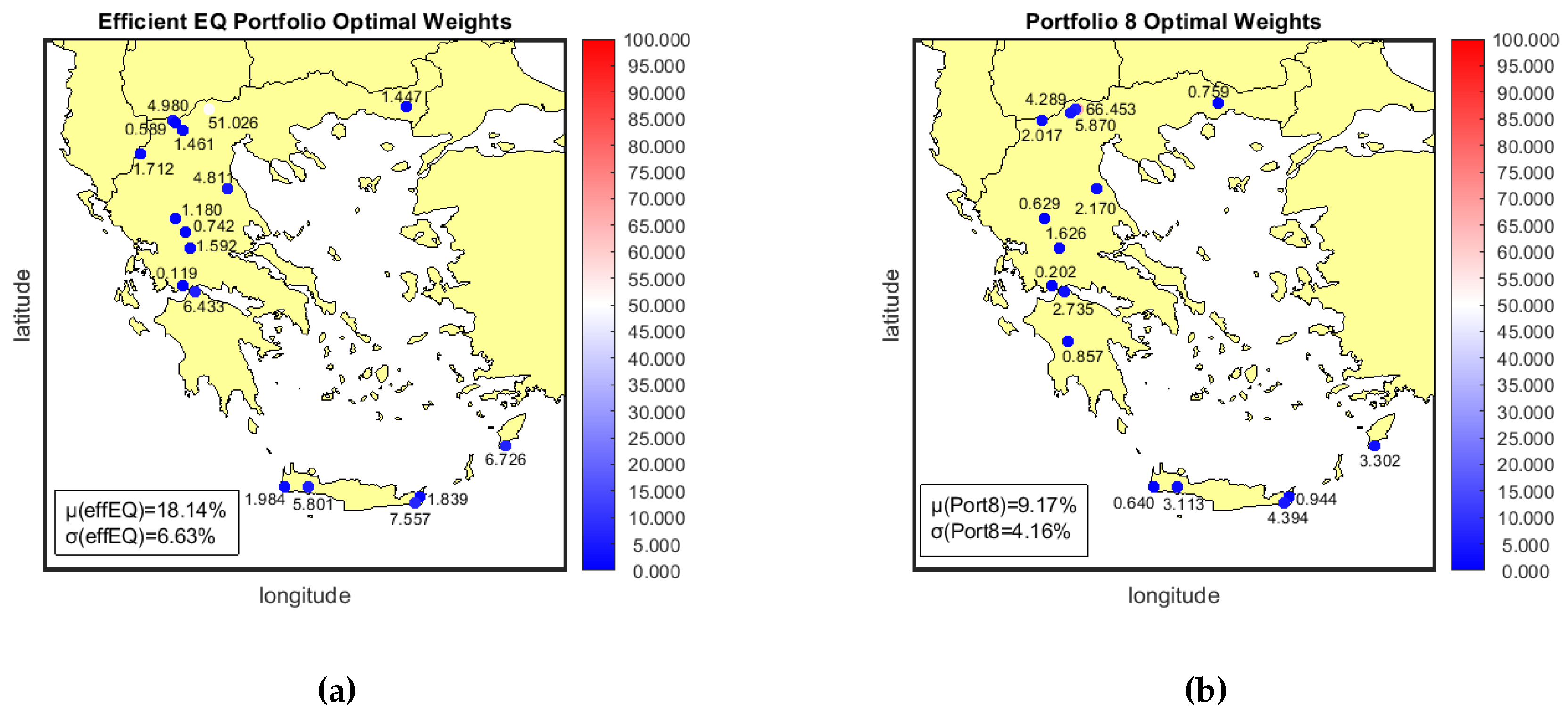
From the 50 efficient portfolios, the minimum value of CV is found on portfolio 33, where . However, even if on that node the relevant is as low as possible for the corresponding , an investor should still has to accept a quite high risk. On the other hand, on portfolio with , the standard deviation is lower and the % increase of daily mean generation for the following portfolios is much higher. Specifically for the 8 first portfolios of the frontier, the % increase of is greater than the % increase of . Thus, portfolio 8 could be a usefull alternative to overcome the low wind generation of the MVP solution. The spatial allocation plan of this portfolio is depicted on Figure 21. In addition to this, the portfolio that has the same mean generation output with the EQ portfolio but with lower volatility is presented on the right of the figure.
Figure 19.
Monthly boxplot for the daily generation capacities of 6 portfolios of the efficient frontier.
Figure 19.
Monthly boxplot for the daily generation capacities of 6 portfolios of the efficient frontier.
Figure 20.
Percentage change on and of 50 portfolios and CV plot.
Figure 20.
Percentage change on and of 50 portfolios and CV plot.
Figure 21.
Alternative portfolios for spatial allocation of wind resources in Greece.
Figure 21.
Alternative portfolios for spatial allocation of wind resources in Greece.
The two portfolios depicted in the maps share common assets with the MVP solution but include additional locations. The Efficient Equally Weighted portfolio comprises a total of 17 areas and portfolio with has 16 assets included. These 2 portfolios have nearly identical selections of locations, differing by only about 2-3 areas.
5.7. Risk Decomposition on the Efficient Portfolios
As a final step in the implementation of an optimal allocation plan, we apply the PCA method to all individual portfolios. However, when conducting PCA on portfolio factor analysis, we cannot employ the same approach as we did for the transformed generating capacities. This is because we must also consider the portfolio weights, which are now a factor influencing the left-hand side of the factor model equation.
Since we have already conducted the PCA analysis for the entire dataset and estimated the factor scores, we can now apply an Ordinary Least Squares (OLS) model. The factor scores will now serve as the independent variables, while the portfolio generation will be the dependent variable. The unknown coefficients in this model are the portfolio loadings, which are valuable for assessing the exposure of the optimal portfolio to the common factors. We can perform a risk decomposition, similar to the one conducted for the entire dataset, specifically for the portfolio case. This allows us to investigate the sources of variability by calculating the total variance explained by the systematic and idiosyncratic components (denoted as
and
correspondingly). The estimated model and the variance decomposition of the portfolio mean generating capacity can be described by the following equations:
The slope coefficients () are the portfolio loadings and is the score of factor k at time t, already computed through PCA in section 5.2. The sign and magnitude of portfolio loadings describe the influence of each systematic risk factor on the portfolio’s generation output. The systematic variance can be computed as the sum of squares of the loadings while the remaining percentage of the total variance accounts for the idiosyncratic variance of the portfolio. The outcomes of the loadings estimation and the risk decomposition are summarized in the following table:
Table 2.
Estimated efficient portfolio loadings of each factor.
Table 2.
Estimated efficient portfolio loadings of each factor.
| Portfolio id |
F1 |
F2 |
F3 |
F4 |
| MV Portfolio |
0.9025 |
0.3054 |
0.6056 |
-0.3945 |
| Portfolio 8 |
0.3539 |
0.1266 |
0.0674 |
-0.1938 |
| EQS Portfolio |
0.3479 |
0.1275 |
0.0507 |
-0.1881 |
| Portfolio 35 |
0.4350 |
0.1706 |
0.0487 |
-0.2567 |
| Portfolio 42 |
0.4574 |
0.2993 |
0.0521 |
-0.3976 |
| MG Portfolio |
0.3043 |
0.7813 |
0.4889 |
-0.7969 |
Table 3.
Risk decomposition of Efficient Portfolios.
Table 3.
Risk decomposition of Efficient Portfolios.
| Portfolio id |
F1 |
F2 |
F3 |
F4 |
Sys.Var |
Idio.Var |
|
|
| MV |
36.13% |
4.14% |
16.26% |
6.90% |
63.46% |
36.54% |
1.32% |
2.87% |
| Portfolio 8 |
46.96% |
6.01% |
1.70% |
14.08% |
69.63% |
30.37% |
9.17% |
4.16% |
| EQS Portfolio |
48.13% |
6.47% |
1.02% |
14.07% |
70.59% |
29.41% |
18.14% |
6.63% |
| Portfolio 35 |
47.86% |
7.36% |
0.60% |
16.67% |
73.53% |
26.47% |
39.45% |
13.33% |
| Portfolio 42 |
33.24% |
14.23% |
0.43% |
25.12% |
74.19% |
25.81% |
47.30% |
16.98% |
| MG Portfolio |
5.92% |
23.51% |
7.90% |
28.11% |
68.95% |
31.05% |
57.39% |
29.13% |
All of the efficient portfolios have a positive loading on the first factor with a moderate value (greater than zero but not very high). This outcome aligns with the loading maps for individual assets in the previous section. The MV portfolio, possesses the highest loading coefficient value for the first factor. The loading coefficients of factors 2 and 3 are also positive for all the portfolios and are higher for MG and MV Portfolio. Finally, all of the portfolios are negatively exposed on the last factor with Portfolio MG to have the higher value. The loading coefficients multiplied with the factor scores determine the direction of the portfolio generation (increase or decrease in each month of the year).
The variance decomposition analysis reveals that the MV Portfolio has the lowest exposure to the systematic component of variance and the highest exposure to the idiosyncratic part, which is not the most favorable scenario. Diversification primarily aims to reduce the idiosyncratic variance by strategically allocating capacity to areas with diverse production profiles. Portfolio 42 has the lowest idiosyncratic variance and the highest level of systematic variance. These findings can be combined with the average daily generating capacity and risk levels to support the decision of a specific spatial allocation plan. For example, the EQS portfolio, previously discussed as an alternative solution, demonstrates lower idiosyncratic risk compared to the MV portfolio, a quite higher generating capacity and moderate levels of volatility.
It is important to emphasize that there is no single definitive answer when it comes to selecting a specific portfolio model, even after employing all the methodologies described in this section. The optimal choice of allocation plan ultimately depends on the risk profile and utility function of the individual investors. Each of the techniques presented here can, however, play a significant role in the decision-making process, providing valuable insights and aiding investors in making informed choices that align with their risk tolerance and objectives.
6. Conclusions and future research
The primary objective of this empirical research was to examine wind generation profiles in onshore areas of Greece and analyze the characteristics of various optimal allocation plans derived by the portfolio optimization process. In examining individual locations, we ascertained that wind farm investments in Greece operate in a manner akin to financial markets where riskier assets are rewarded with higher power generation levels. Combining these assets within a portfolio results in reduced volatility and a more stable production throughout the year. Furthermore, our analysis led us to the inference that the cardinality of the optimal solutions in the efficient frontier is exceptionally low regarding the asset universe. This, in turn, can lead to optimized investment costs compared to a naive selection of assets. However, it was found that the MVP solution is not always the best option, even for an exceedingly conservative investor due to the ’no-free-lunch property’ that drops the wind generation to near-zero levels. Empirical distributions of portfolios lying in the first half of the efficient frontier are right-skewed with a substantial portion of the probability mass clustered around zero values. Nonetheless, due to the relative steep slope of the efficient frontier, higher generation outputs can be achieved with only a marginal increase in risk.
Descriptive statistics and various graphical representations were utilized, including timeplots and boxplots, to evaluate specific portfolios of the efficient frontier. Starting from the MV portfolio, the 8th and the EQS portfolio were identified as potential alternatives offering higher generation with a slight increase on risk that could be deployed as the final spatial allocation plan. A more in-depth understanding of the qualitative characteristics of the designated efficient portfolios was addressed through Factor model and PCA estimation. The model evaluation criteria proposed 4 systematic risk factors that impact production across all areas with different exposures. The first factor is non-diversifiable while all the others can be diversified away with a proper area selection method. The production pattern undergoes significant changes during the summer and winter seasons, with the loading sign becoming a critical determinant of generating capacity outcomes. For a more comprehensive explanation, reconstruct analysis was deployed to isolate and reveal the effect that each systematic factor has in the overall wind generation.
Management of Renewable Energy Sources is a contemporary topic that has gained prominence in academic literature in recent years and remains an open field for future research. Our study could be further expanded in several topics and address similar challenges. For instance, the complementarity of resources, although studied in a number of papers, it could still hold the potential for valuable insights for the Greek territory. The integration of wind and solar energy sources can enhance and stabilize annual generation while simultaneously reducing volatility and the zero-production occurrences of a portfolio of wind farms. [
31,
52,
53]. Moreover, the portfolio configuration offers flexibility for various modifications that can address diverse problems. For example, some studies define the different production technologies as individual assets and focus on deriving an optimal energy mixture tailored to specific geographical areas. [
29,
30].
An other direction is the examination of different strategies to mitigate the volumetric risk of renewable energy such as hedging strategies. Wind Power Futures and other financial contracts are steadily launched by EEX and attract potential investors [
8,
54,
55,
56]. The market is on a premature level and scientific research has the potential to pave the way for the development of new derivatives designed to capture various dimensions of volumetric risk [
7,
57]. In addition, future studies could broaden their scope to encompass even larger geographical areas, such as entire continents, or delve into the interconnection challenges between multiple continents to address optimization problems in spatial resource allocation, accounting for constraints such as transmission capacity. Lastly, a holistic examination of both the demand and supply sides can provide a more comprehensive understanding of the energy markets functionality.
