CMIP5 Decadal Precipitation at Catchment Level

The fidelity of the decadal experiment in Coupled Model Intercomparison Project Phase-5 (CMIP5) has been examined, over different climate variables for different temporal and spatial scales, in many previous studies. However, most of the studies were for the temperature and temperature-based climate indices. A quite limited study was conducted on precipitation of decadal experiment and no attention was paid to a catchment level. This study evaluates the performances of eight GCMs (MIROC4h, EC-EARTH, MRI-CGCM3, MPI-ESM-MR, MPI-ESM-LR, MIROC5, CMCC-CM, and CanCM4) for the monthly hindcast precipitation of decadal experiment over the Brisbane River catchment in Queensland, Australia. First, the GCMs datasets were spatially interpolated onto a spatial resolution of 0.050×0.050 (5 km× 5 km) matching with the grids of observed data and then were cut for the catchment. Next, model outputs are evaluated for temporal skills, dry and wet periods, and total precipitation (over time and space) based on the observed values. Skill test results reveal that model performances varied over the initialization years and showed comparatively higher scores from the initialization year 1990 and onward. Models with finer spatial resolutions show comparatively better performances as opposed to the models of coarse spatial resolutions where MIROC4h outperformed followed by EC-EARTH and MRI-CGCM3. Comparing the skills, models are divided into three categories (Category-I: MIROC4h, EC-EARTH, and MRI-CGCM3; Category-II: MPI-ESM-LR and MPI-ESM-MR; and Category-III: MIROC5, CanCM4, and CMCC-CM). Three multimodel ensembles’ mean (MMEMs) are formed using the arithmetic mean of Category-I (MMEM1), Category-I and II (MMEM2), and all eight models (MMEM3). The performances of MMEMs are also assessed using the same skill tests and MMEM2 performed best which suggests evaluating the models before the formation of MMEM.

Keywords:

Subject: Environmental and Earth Sciences - Other

1. Introduction

Evaluation of General Circulation Models (GCMs) has become a very important task to measure the models’ credibility in future prediction of climate variables. Evaluation of models predicted historical data based on their corresponding observed values determines how well the GCMs represent historical climate and thus forms an integral part of the confidence-building exercise for climate predictions. It is assumed that the better performance of models over the historical period leads to developing more confidence in their future predictions. As the GCMs are used to explore the future climate variabilities and potential impacts on the Earth, evaluation of GCMs has been a growing need in the climate research community. However, depending on the requirements, available resources, geographical locations, and variables considered to assess the model performances, the evaluation strategies become different. Since the change of climate and its potential impact on this planet varies from region to region, it is important to evaluate the models based on different regions and spatial scales though the evaluation of climate models and their ensembles is crucial in climate studies [1]. Research on regional or local climate variability and their potential impacts are high in demand for transferring research-based scientific knowledge to increase the resilience of society to climate change. This will help in planning the future development of the infrastructures of a region [2].

Coupled Model Inter-comparison Project Phase-5 (CMIP5) provides an unprecedented collection of global climate data of different time scales including decadal experiments that were produced by a wide range of GCMs [3]. Evaluation of CMIP5 decadal prediction has been run so far based on different evaluation aspects such as different regions, different climate variables, and their different spatial and temporal resolutions. For instance, Choi et al. [4] investigated the prediction skill of CMIP5 decadal hindcast near-surface air temperature for the global scale while other researchers investigated other climate variables in continental or regional scales [5,6,7]. Lovino et al. [5] evaluated decadal hindcast precipitation and temperature over northern Argentina and reported higher skills of models to reproduce the temperature as opposed to precipitation where precipitation skills were found remarkably lower. Mckeller et al. [6] investigated decadal hindcast maximum and minimum temperature over the state of California and reported the best-performing model. Likewise, Gaetani and Mohino [7] evaluated model performances to reproduce Sahelian precipitation and reported better-performing models. However, these studies were for different geographical locations with coarser spatial resolutions for considered variables. For instance, the spatial resolution of models used by Kumar et al. [2] and Choi et al. [4] was 2.5⁰, Gaetani and Mohino [7] used models of more than 1.1⁰, and Lovino et al. [5] used precipitation data of 1.0⁰ spatial resolution. At a regional level, Mehrotra et al. [8] assessed the multi-model decadal hindcast of precipitation for different hydrological regions over Australia using 0.5⁰ spatial resolution and reported lower skills for precipitation as opposed to temperature and geopotential height. Climate data of 0.5⁰ spatial resolution covers a ground area equivalent to a square of 50 km length over the Australian region. Comparatively, a 50 km × 50 km area is very big where climate variabilities are also large and frequency and magnitude of precipitation vary in a few kilometers (such as in Australia). As the precipitation shows more spatial and temporal variability than temperature and the model performances vary from region to region, therefore the model performances at the local level for finer spatial resolution are essential for precipitation.

Numerous studies evaluated CMIP5 models over Australia [5,6,7] but studies on evaluating CMIP5 decadal precipitation at catchment scale can hardly be found. After Mehrotra et al. [8], who assessed the CMIP5 decadal hindcast precipitation over different hydrological regions (0.5⁰ ×.0.5⁰) in Australia, recently Hossain et al. [5,6,7] used the CMIP5 decadal precipitation at a further finer resolution of 0.05⁰ ×0.05⁰ (5km×5km) for Brisbane River catchment Australia for the first time. Hossain et al. [5,6,7] compared the model performances for investigating the model drift and their subsequent correction using alternative drift correction methods for both the monthly and seasonal mean precipitation. However, they compared the model performances at a single grid point within the Brisbane River catchment. On the contrary, Mehrotra et al. [8] used only a multi-model approach but did not consider individual models finer than 0.5⁰ spatial resolution. Local climate variables of finer temporal and spatial resolution, especially for precipitation, are very important for water managers for planning and developing infrastructures as well as decision-making for local businesses and agriculture. To maintain sustainable development with effective future planning based on the models’ projected precipitation, it is important to evaluate the performance of the CMIP5 models’ hindcast precipitation.

Many researchers have suggested using MMEM [14,15,16,17] while using GCM data to reduce the model biases. The use of MMEM may enhance the model performances [14,15,16,17] by reducing the biases to some extent but there is no information available on the ranking of GCM models and based on this, which and how many models should be considered to produce MMEM so that it could provide better outcome. This is essential for CMIP5 decadal precipitation because of its wide range in spatial and temporal variability in providing the model output ten years ahead. That is why the objective of this paper is, first, to categorize the models based on their performances at the catchment level with a spatial resolution of 0.05⁰ and next, to identify the best combination of different models that would provide better performance. This would help the water managers and policymakers to sort out models depending on their specific needs while assessing the future water availability based on the GCMs-derived precipitation on a decadal scale through CMIP5.

2. Data Collection and Processing

2.1. Data Collection

CMIP5 decadal experiment provides 10 and 30-year-long ensemble predictions from multiple modeling groups [henceforth mentioned as CMIP5 decadal hindcasts, [19]]. Monthly decadal hindcasts precipitation from eight GCMs (out of ten); MIROC4h, EC-EARTH, MRI-CGCM3, MPI-ESM-MR, MPI-ESM-LR, MIROC5, CMCC-CM, and CanCM4 for which decadal hindcast precipitation are downloaded from CMIP5 data portal (https://esgf-node.llnl.gov/projects/cmip5/). The other two models, HadCM3 (spatial resolution 3.75° x 2.5°) and IPSL-CM5A-LR (spatial resolution 3.75° x 1.89°) were not considered in this study because of their relatively coarser spatial resolution and different calendar system (HadCM3). For the initialized period 1960-2005, data simulated over 10 years that are initialized every five years during this period are selected for this study as they were found comparatively better than the 30-year simulation [20]. The details of the selected models are given in Table 1.

The observed gridded monthly precipitation of 0.050 ×.0.050 (≈ 5km × 5km) was collected from the Australian Bureau of Meteorology (Observed/Bureau). This data was produced using the Australian Water Resources Assessment Landscape model (AWRA-L V5) [21].

2.2. Data Processing

The GCMs’ resolutions (100-250 km) are found inadequate for regional studies due to lack of information at catchment levels [22,23,24]. The regional climate model (RCM) is useful to transfer the coarse spatial GCMs’ data to local scale but it needs a wide range of climate variables as well as rigorous efforts to develop. For this reason, GCMs data are spatially interpolated onto 0.05⁰×0.05⁰ spatial resolution using the second-order conservative (SOC) method matching with the grids of observed data. For the gridded precipitation data, the SOC method was found comparatively better than other commonly used spatial interpolation methods [25]. Skelly and Henderson-Sellers [26] suggested GCM derive gridded precipitation to consider as areal quantities and spatial interpolation will not create any new information except the spatial precision of the data. Skelly and Henderson-Sellers [26] also suggested that researchers could subdivide the grid box in almost any manner until the original volume remains the same. On the contrary, Jones [27] suggested that precipitation flux must be remapped in a conservative manner to maintain the water budget of the coupled climate system. While sub-gridding the GCM data using the SOC method, it conserves precipitation flux from their native grids to subsequent grids [27]. For this reason, this study used the SOC method for spatial interpolation as it was followed in other research [13]. Brisbane River catchment was selected for this study because of its tropical climate that produces low to moderate variability of annual precipitation values.

3. Methodology

A simple and direct approach for the model evaluation is to compare the model output with the observations and analyze the differences. In this study, models are evaluated for temporal skills, dry and wet periods, and total precipitation based on the observed values. Here, CC, ACC, and IA are used to measure the temporal skills, FSS are used to measure the skills over dry and wet periods, field-sum and total-sum are used to measure the skills for total precipitation. There are 496 grids in the Brisbane River catchment with a spatial resolution of 5.0 km × 5.0 km. The descriptions of the skills are given below.

3.1. Correlation Coefficient (CC)

CC measures the linear association and presents the scale of temporal agreement between predicted and observed values. Statistically, it measures how much closer the scatter plot points to a straight line. CC ranges from -1 to 1 for no to perfect correlation respectively.

C C = \frac{\sum (F_{i} - \bar{F}) (O_{i} - \bar{O})}{\sqrt{\sum {(F_{i} - \bar{F})}^{2}} \sqrt{\sum {(O_{i} - \bar{O})}^{2}}}

(1)

Here,

F

and

\bar{F},

represent models’ predicted and their mean whereas

O

and

\bar{O}

represent observed precipitation and their mean respectively. In the following skill tests, these notations will remain the same. Note that the mean is calculated for every individual year.

3.2. Anomaly Correlation Coefficient (ACC)

ACC was suggested by Wilks [28] to measure the temporal correlation between anomalies of the observed and predicted values. For the verification of numerical weather models’ prediction ACC is frequently used. Its value ranges from -1 to 1 for no to perfect anomaly matching.

A C C = \frac{\sum \{(F_{i} - C) - (\bar{F - C})\} * {(O_{i} - C) - (\bar{O - C})}}{\sqrt{\sum {(F_{i} - C)}^{2}} \sqrt{\sum {(O_{i} - C)}^{2}}}

(2)

Here, C represents the mean of the entire time-span (ten years) of the observed (Bureau) data. The higher value of ACC will indicate the higher performance in reproducing the monthly anomalies.

3.3. Index of agreement (IA)

Wilmot [29] suggested IA to measure the accuracy of predictions. The index of agreement can be calculated as follows.

I A = 1 - \frac{\sum_{i = 1}^{n} {(F_{i} - O_{i})}^{2}}{\sum_{i = 1}^{n} ({|F_{i} - \bar{O}| + |O_{i} - \bar{O}|)}^{2}} .

(3)

The index is bounded between 0 and 1 (0≤IA≤ 1). The value closer to 1 indicates the most efficient predicting of the models.

3.4. Fractional Skill Score (FSS)

FSS is a grid-box event that directly compares the fractional coverage of models’ predicted and observed values for the entire catchment. It measures how the spatial variability of models’ predicted values corresponds to the spatial variability of the observed values. FSS can be obtained as:

F S S = 1 - \frac{\frac{1}{N} \sum_{N} {(P_{f, m} - P_{f, o})}^{2}}{\frac{1}{N} [\sum_{N} P_{f, m}^{2} + \sum_{N} P_{f, o}^{2}]}

(4)

Where

P_{f}

and N refers to calculated fraction and number of years respectively. The subscript m and o present modeled and observed respectively. In this study, fractions are calculated according to Roberts and Lean [30] but considered entire catchment as a whole unit, and the temporal averages (for considered months) are taken instead of the spatial averages. For doing this, threshold values; ≥85 percentile for the months of wet seasons (December to February -DJF) and <15 percentile for the months of the dry seasons (June to August - JJA) are considered. To get the fractions (say for January), the number of grid points covered for a specified threshold value is counted and then divided by the total number of grids within the catchment. The differences between predicted and observed fractions (the numerators of equation 4) are calculated for individual months. The FSS is a temporal average score for the catchment for each considered month. It ranges from 0 to 1 for no to perfect match respectively.

3.5. Field-sum and total-sum

Models’ ability to reproduce the total precipitation over the entire catchment is considered as the spatial skills of the models. Field-sum is the sum of precipitation over the entire catchment for individual time steps and the total-sum is the field-sum over the total time span. Field-sum and total-sum of the models’ precipitation are compared with the corresponding observed values.

4. Results and Analysis

4.1. Temporal skills

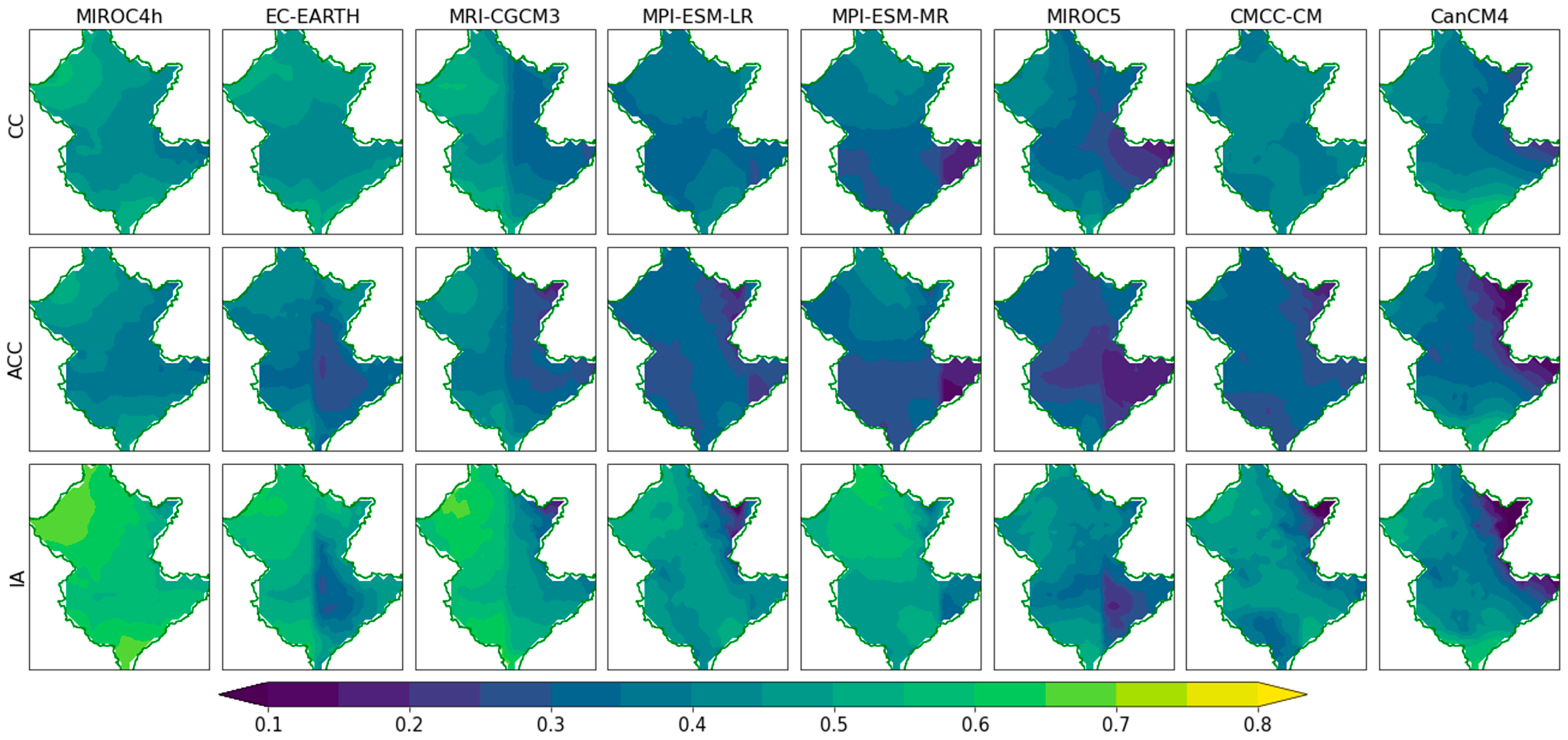
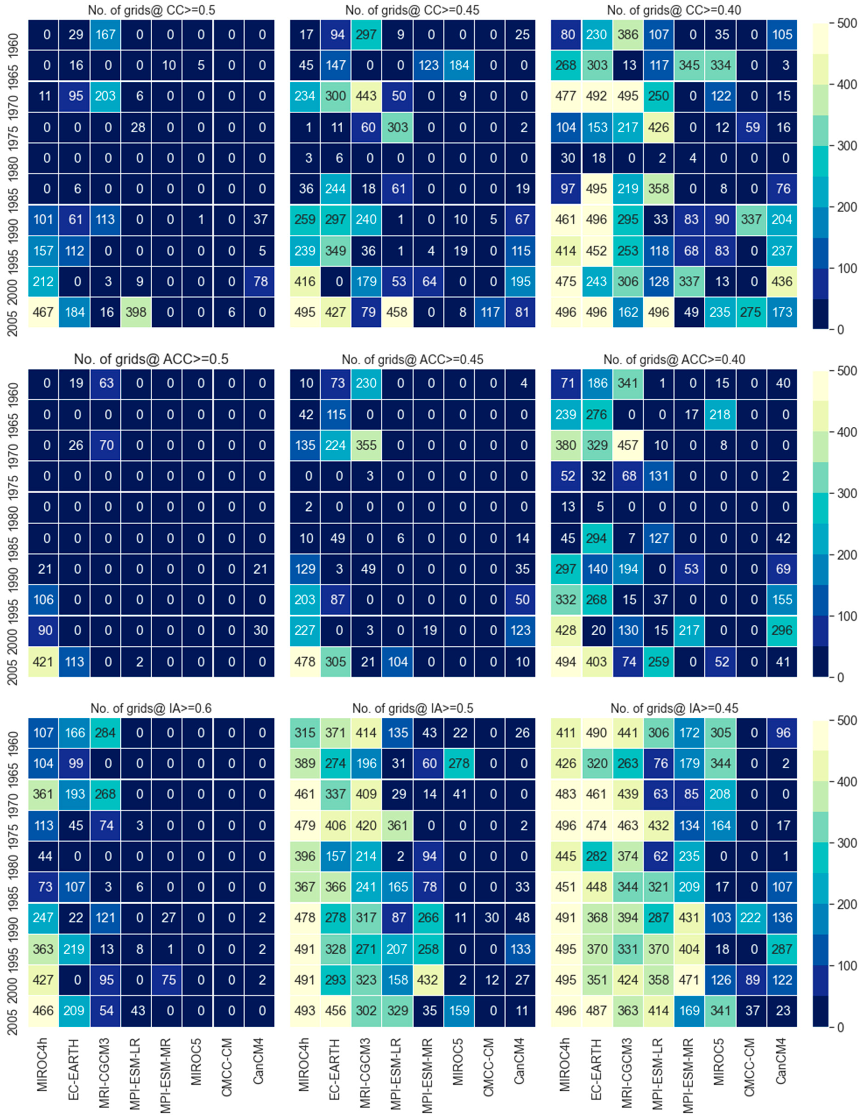
The temporal skills are computed at every individual grid (total 496 grids) of the catchment for all initialization years of each model. Spatial variations of models’ temporal skills across the catchment for the initialization year 1990 (1991-2000) are presented in Figure 1. The models are evaluated from the spatial perspective by counting the number of grids covered by different models for different threshold values of CC, ACC, and IA Figure 2. The higher number of grids represents the higher spatial skill of models across the catchment. From the comparison of temporal skills, it is evident that model performance varies over the initialization years and also across the catchment. From the initialization year 1990 and onward, all models show a comparatively higher number of grids for the same thresholds of CC, ACC, and IA and the lowest skill observed in 1980. With the increase of threshold values, the number of grids declines for all models in all three temporal skills except CMCC-CM and MIROC5 in ACC. Compared to other selected models, MIROC4h, EC-EARTH, and MRI-CGCM3 show a higher number of grids for all thresholds in which MIROC4h is much ahead of EC-EARTH and MRI-CGCM3. It means temporal agreement, the resemblance of anomalies, and the prediction accuracy of MIROC4h and EC-EARTH spatially higher than other models. This study also checked the number of grids for the threshold >=0.6 for CC and ACC but no model could reproduce CC and ACC >=0.6 at any grid. However, MIROC4h, EC-EARTH, and MRI-CGCM3 show a significant number of grids for the IA threshold >=0.6 where MIROC4h outperformed EC-EARTH and MRI-CGCM3 (Figure 2). Comparing the models, MIROC4h shows higher temporal skills from the spatial perspective, followed by EC-EARTH and MRI-CGCM3 whilst MPI-ESM-MR, MIROC5, and CMCC-CM show low to lowest temporal skills. Over the catchment MIROC5, MPI-ESM-MR, CanCM4 show little better scores than CMCC-CM.

4.2. Evaluation for dry and wet periods

Skills to reproduce the dry and wet events are assessed at the selected grid and also over the entire catchment. For the selected grid all months are considered against four different thresholds (25, 50, 75, and 90 percentiles correspond to 25, 60, 110, and 175 mm respectively) whereas for the entire catchment, FSS are used for the months of dry (JJA) and wet (DJF) periods only.

4.2.1. At the selected grid

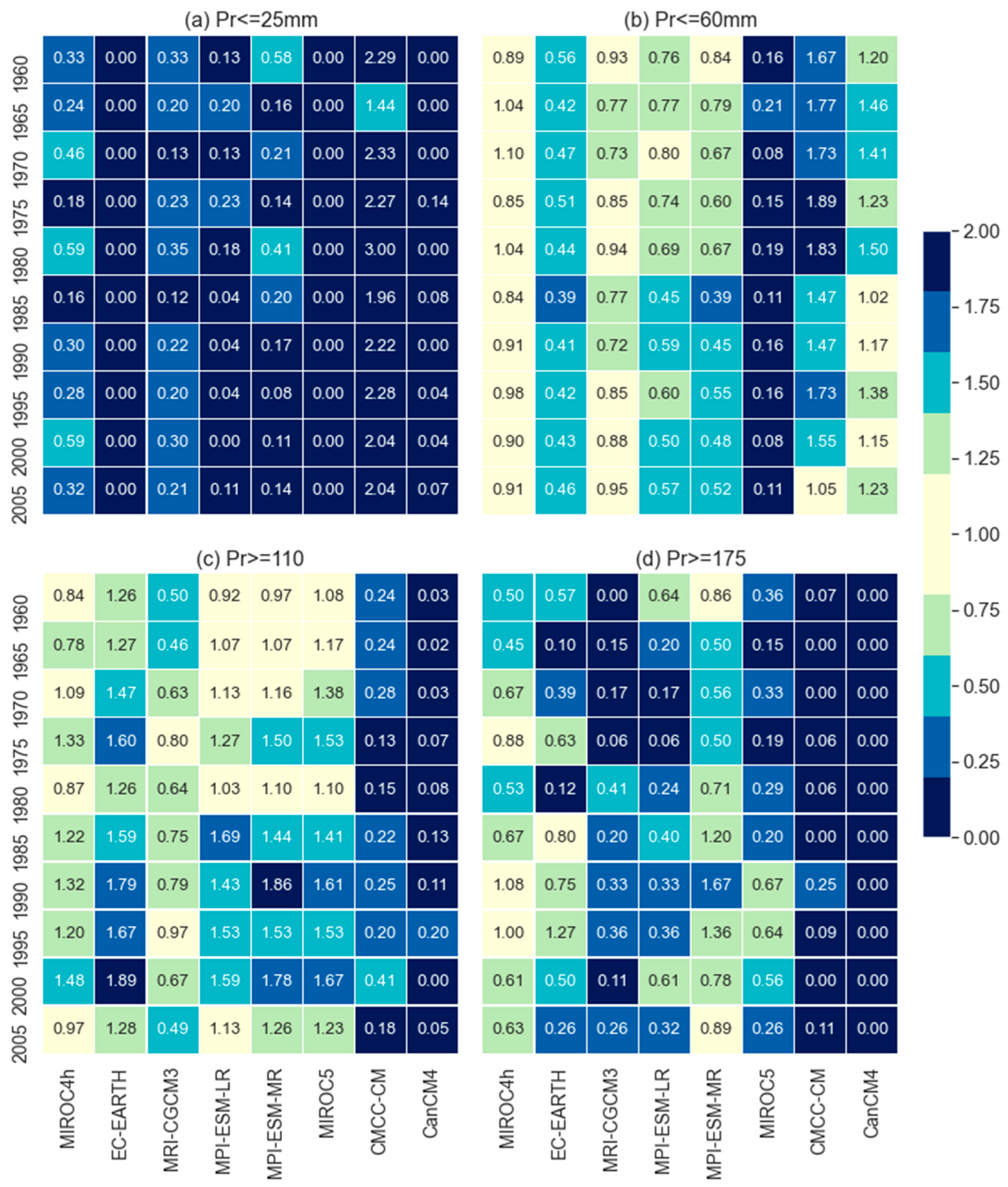
A comparison to reproduce the dry and wet events based on the selected precipitation thresholds at the selected grid is presented in Figure 3. This comparison was based on the ratio of the number of months of respective precipitation thresholds (mentioned on the top of the individual plot in Figure 3.) in model data to observed data. It is observed that EC-EARTH and MIROC5 could reproduce no dry events (Pr<=25 mm) whilst CMCC-CM overestimates the number of dry events which is almost double the dry events in observed data. Meanwhile, MIROC4h performed better to produce dry events as well as 50 and 75 percentile values as compared with the other models. However, MIROC4h is a little behind the MPI-ESM-MR for the extreme wet events (Pr>=175 mm). It means MPI-ESM-MR can reproduce extreme wet events better than the other models. EC-EARTH, MPI-ESM-LR, and MPI-ESM-MR underestimated the events of threshold Pr<=60mm whereas overestimated the wet events (Pr>=110 mm) which is an indication of models’ tendency to reproduce a higher number of wet events than opposed to dry. However, MRI-CGCM3 performed similarly to MIROC4h in reproducing the number of events for the threshold of <= 60mm but underestimated the number of events thresholds of >= 110mm. To reproduce the extreme wet events (Pr>=175 mm), all models show underestimation in which MPI-ESM-MR and MIROC4h showed considerably better skills. The CMCC-CM and CanCM4 showed poorest, and no skill respectively for extreme wet events.

4.2.2. Over the entire catchment

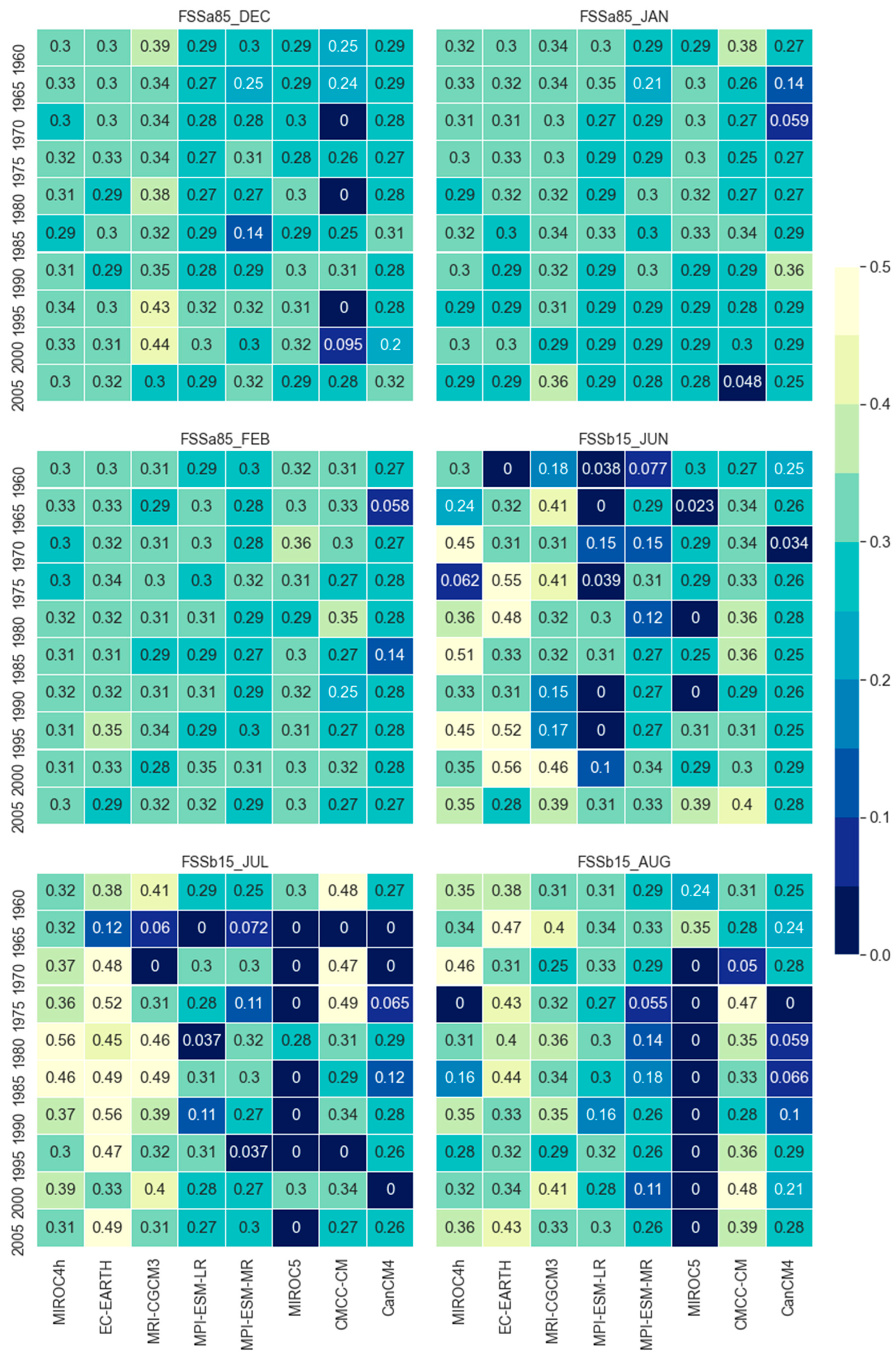
FSSs are calculated for the months of winter (dry) and summer (wet) seasons only. FSS of all the initialization year of all models are shown in Figure 4. Results show that for the months of summer seasons (DJF), MRI-CGCM3 shows higher skills in December and January but little behind than EC-EARTH in February. On the contrary, CMCC-CM shows the lowest skill in December but shows similar skill with other models in January and February.

However, except higher skill of MRI-CGCM3 and the lowest skill of CMCC-CM in December, all other models show similar skill scores with few variations in winter seasons. This indicates different models’ skills are almost similar to reproducing wet events. In the dry season, MIROC5 shows the lowest skill while EC-EARTH shows the higher skills, which is even higher than MIROC4h and MRI-CGCM3. The FSSb15 scores of EC-EARTH, MIROC4h, and MRI-CGCM3 are much better than the score obtained for FSSa85. This reveals that these models are better to reproduce dry events as opposed to wet events and the reverse is true for MIROC5, MPI-ESM-MR, and CanCM4 respectively.

4.3. Evaluation for total precipitation

4.3.1. At the selected grid

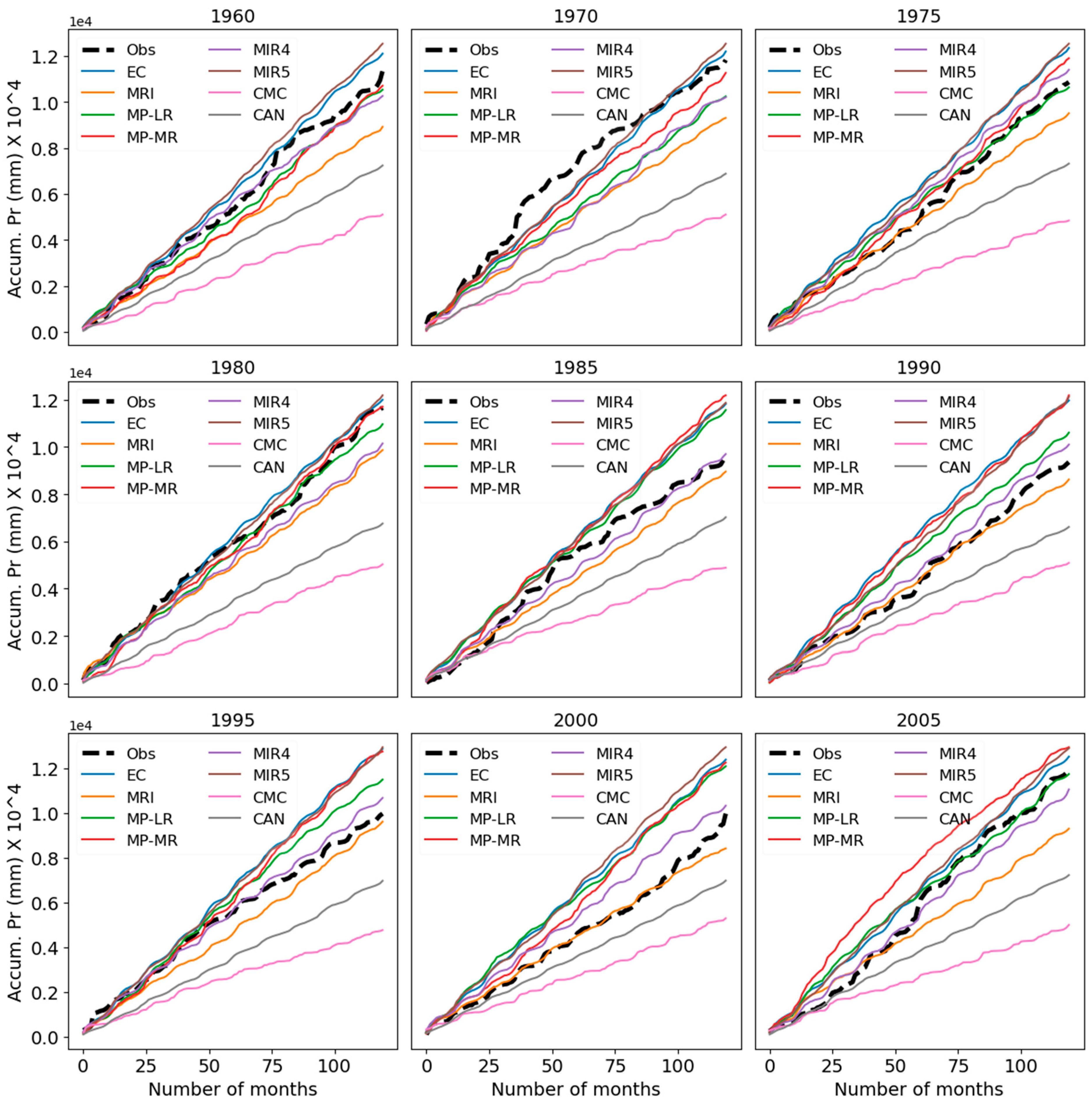
To evaluate the model performances in reproducing the total precipitation, models’ cumulative (over time) precipitation at several randomly selected grids (evenly distributed across the catchment) within the catchments and total precipitation over the entire catchment are compared. The cumulative sum of monthly precipitation of different models at the selected grid for different initialization years is presented in Figure 5. The model skills show both temporal and spatial variations in predicting accumulated precipitation but no model could reproduce the accumulated precipitation as observed. However, only a few models (MIROC4h, MPI-ESM-LR, and MPI-ESM-MR) could reproduce the accumulated precipitation close to the observed accumulation. Nevertheless, CMCC-CM, CanCM4, and MRI-CGCM3 underestimated the accumulated precipitation whilst EC-EARTH and MIROC5 overestimated the accumulated values. With the change of grid locations, model performances may change but the relative performances among the models will remain the same.

4.3.2. Over the entire catchment

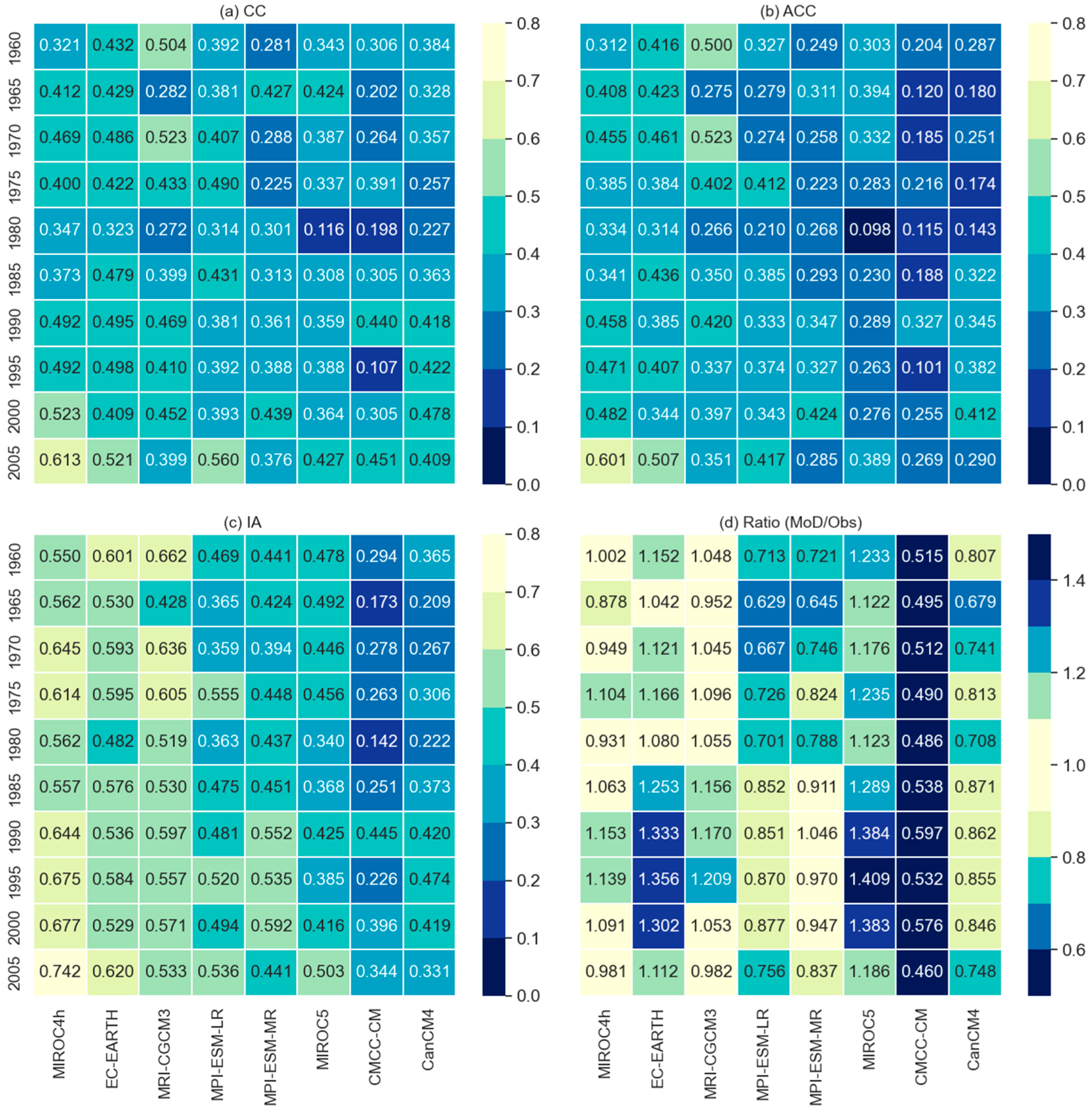
For comparing the model performances on total precipitation over the entire catchment, this study calculated the field-sum of the models and observed values then assessed through the temporal skills as shown in Figure 6. The total sum of the models and observed values are also calculated and assessed through the ratio between model and observed values (Figure 6). From the comparison, it is observed that the field sum of MIROC4h, EC-EARTH, and MRI-CGCM3 show comparatively higher accuracy (IA), temporal agreement (CC), and the resemblance of anomalies (ACC) with the field-sum of the observed precipitation. The model performances on reproducing the total precipitation vary over the initialization years (Figure 6d).

Before and after 1985, MRI-CGCM3 and MPI-ESM-MR showed comparatively better resemblance with the observed total precipitation followed by MIROC4h and EC-EARTH. On the contrary, CMCC-CM showed the lowest performance to reproduce total-sum precipitation throughout all initialization years. From the skill assessments, it is revealed that the MIROC4h surpasses other models in almost all performance indicators followed by EC-EARTH and MRI-CGCM3 whilst MPI-ESM-LR and MPI-ESM-MR show medium skill scores. Lower skill scores were observed for MIROC5, CanCM4, and CMCC-CM respectively. MIROC4h was also marked as the best model to reproduce precipitation in other studies [22,23,24] though they did not use the decadal experiments data. It may be due to the finer resolution of the atmospheric component of MIROC4h that enhanced its ability to capture the more realistic climate features [22,23,24] at the local level.

The overall skill assessment results revealed that all models show comparatively lower skills in the initialization years 1960 to 1985 and better skills observed from the initialization year 1990 and onward.

4.4. Model categorisation and formulation of MMEM

Based on the skill comparisons, this study divided the models into three different categories; Category-I, Category-II, and Category-III. While categorizing the models based on their skills at the selected grid and over the catchment, MIROC4h, EC-EARTH, and MRI-CGCM3 fall in the first category (Category-I) as they consistently performed in the top three and their performance metrics were found very close to each other. Similarly, MPI-ESM-LR and MPI-ESM-MR are in the second (Category-II) category as they have shown medium skill scores in all skill tests over the initialization years. Lastly, MIROC5, CanCM4, and CMCC-CM fall in Category-III.

GCMs’ outputs indeed contain uncertainties and biases which will cause the lower skill score but multi-model ensembles mean (MMEM) may enhance the models’ skills [22,23,24] by reducing uncertainties [22,23,24]. In this study, the skill tests are employed on the ensembles’ mean of individual models’ raw values (interpolated) only. Here the arithmetic mean of multiple models has referred to as MMEM. The performances of MMEMs were also assessed based on the similar skill tests that are employed on individual models and the results are summarized below. To form the MMEMs, three different combinations are considered. The arithmetic mean of Category-I models is referred to as first MMEM (MMEM1), the arithmetic mean of the Category-I and Category-II models is referred to as the second MMEM (MMEM2) and finally arithmetic mean of all models is referred to as the third MMEM (MMEM3).

4.5. Performance of MMEMs

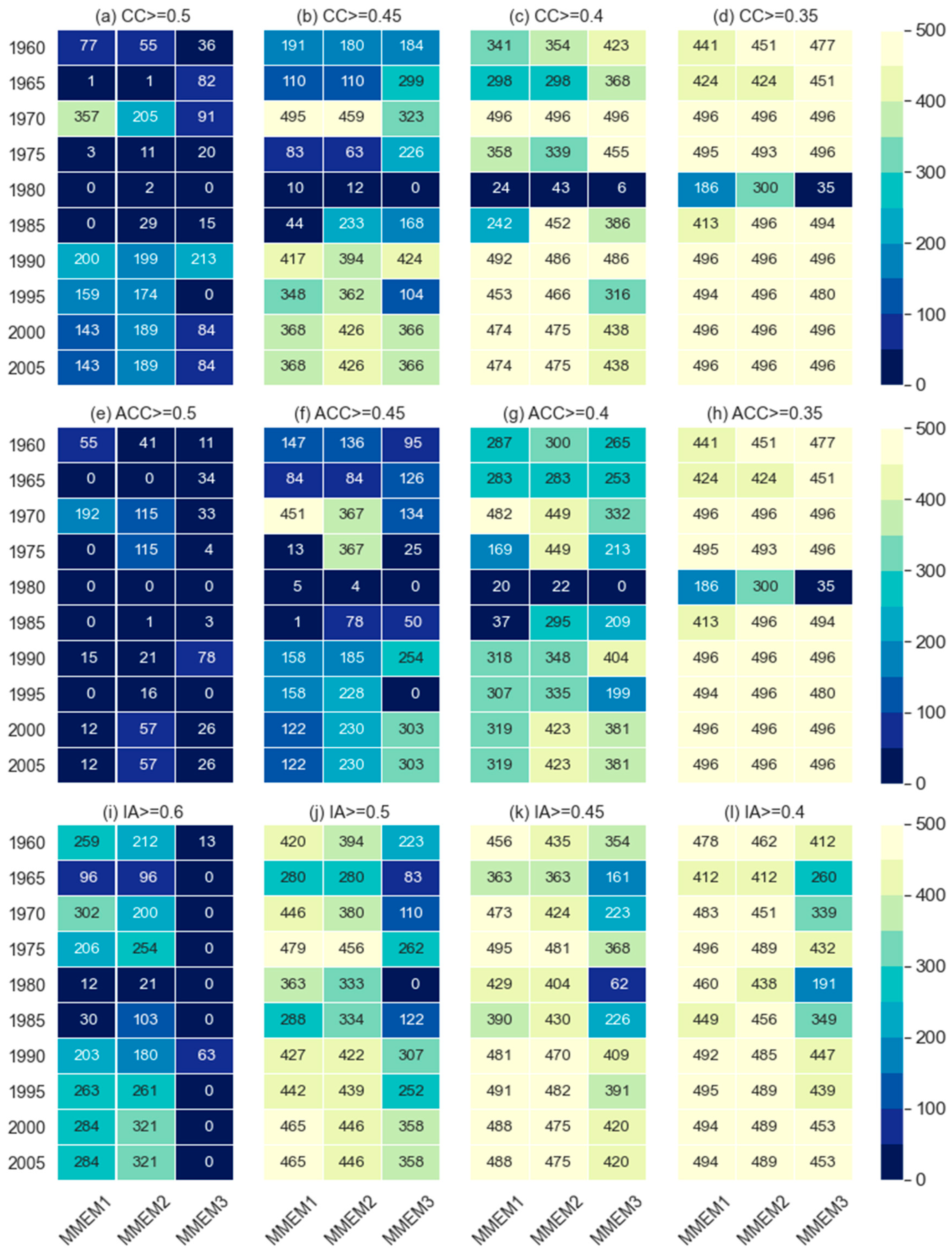
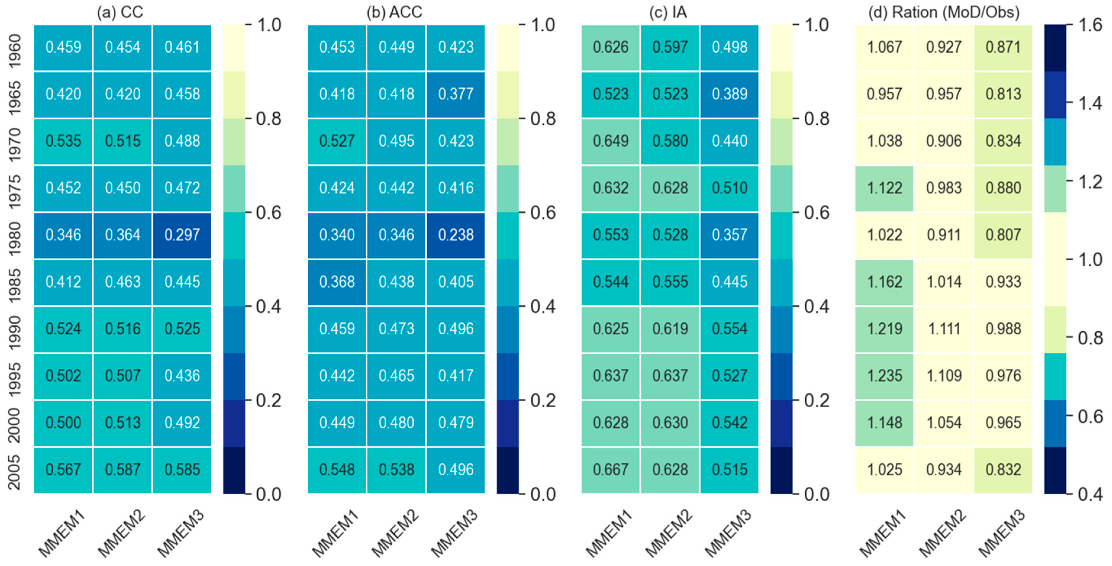
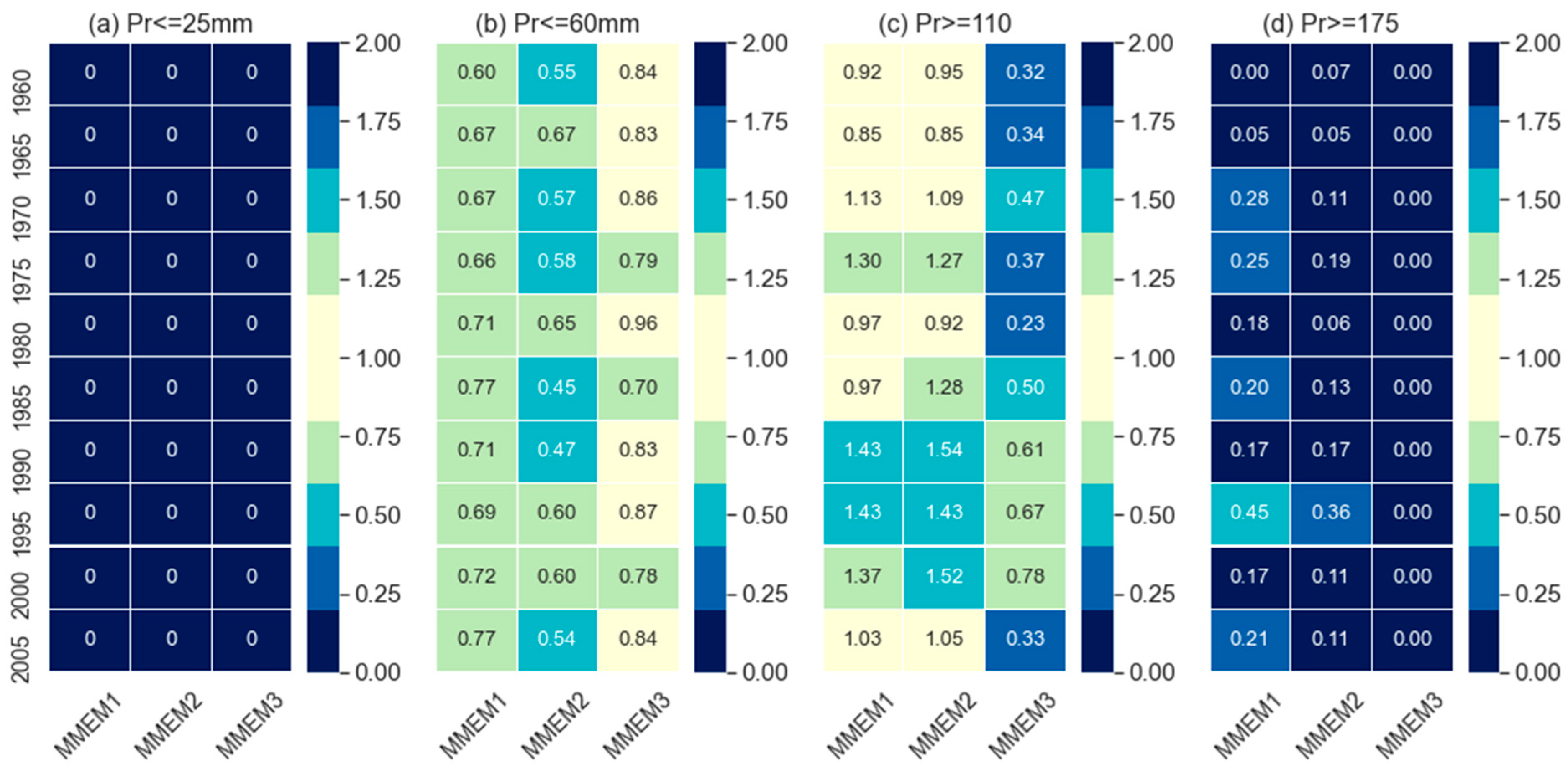
The temporal skills at individual grids of the different thresholds, temporal skills along with the ratios of the field-sum, and skill on reproducing dry and wet events of different thresholds for MMEMs are presented in Figure 7, 8 and 9 respectively. In general, MMEMs show better performance than the individual models for comparatively lower thresholds of the performance metrics. For instance, the MIROC4h model showed the highest number of grids for CC and ACC at the threshold 0.5 (Figure 2) but no MMEMs could reproduce this number of grids at the same threshold (Figure 7). The same results were also observed for IA at the threshold 0.6 (see Figure 7i) but for the lower thresholds, MMEM2 shows better skill than MIROC4h in CC and ACC but not in IA. Among the three combinations, MMEM2 surpasses the other two combinations in reproducing CC and ACC. Nevertheless, in the case of IA, MMEM2 is little behind than MMEM1. Similar results are evident for performance indicators obtained from the field-sum of MMEM and the observed values (Figure 8), where MMEM2 shows best for the CC and ACC but both MMEM2 and MMEM1 show similar skills for IA. However, to produce the dry and wet events, MMEMs show lower performance as compared to individual models. For instance, MIROC4h, MRI-CGCM3, and MPI-ESM-MR captured some dry events (Pr<=25mm) at the selected grid point (Figure 3) but no combination could capture it (Figure 9) whilst for the wet events, MMEM shows very poor skills.

Meanwhile, MMEMs show better performance indicators (CC, ACC, and IA) for the total precipitation of the entire catchment (field-sum) which is even better than the individual models. Nevertheless, MMEM is a little behind the MIROC4h and MRI-CGCM3 for the ratio of total-sum (sum over total time span and catchment) model combinations over the corresponding observed values (see Figure 5d).

5. Discussion

This study evaluated the performance of eight selected GCMs simulation of CMIP5 decadal precipitation at a catchment level of 0.05-degree spatial resolution. Different skill metrics were employed from both temporal and spatial perspectives in this evaluation assessment. The performance metrics; CC, ACC, and IA measured the temporal skills of the models. The number of grids corresponding to individual metrics’ thresholds represents the spatial skills of the models. These metrics are also calculated for the spatial sum (sum over the entire catchment) of the precipitation for all models. In addition to these, FSSa85 and FSSb15 presented the spatial skill of the models for wet and dry seasons respectively. The CC and ACC measured the phase and correspondence (or anomalies) of the model time series concerning the observed values. The models showed a wide range of performance scores over the initialization years as well as across the catchments. It may be due to the difference in understanding of models on local climate features or the precipitation data of finer temporal and spatial resolutions or the combination of both.

Indeed, the model performances are dependent on the model assumptions or basic principle on understanding the earth climate system, its processes, and interactions among atmosphere, oceans, land, and ice-covered regions of the planet. Besides them, decadal prediction skill also depends on the method of model initialization, and quality and coverage of the ocean observations [3]. Different initializations also may cause models’ internal variability that is still open for further discussion. For the decadal prediction, one of the most important aspects is the model drift and its correction [8]. However, to evaluate the performance of models’ derived raw data, neither the drifts were investigated nor any drift correction methods are employed. The reason is, the drift correction method itself may introduce additional errors that may not reflect the real performance of the models [22,23,24]. Based on the understanding of physical, chemical, and biological mechanisms of earth systems, different modeling groups have come up with different models with reproducing capabilities of climate variables that may vary over different regions [22,23,24] and climate variables [22,23,24]. For instance, Kumar et al. [2] analyzed the precipitation and temperature trends of the twentieth century from nineteen CMIP5 models and reported that the models’ relative performances are better for temperature as opposed to precipitation trends. Generally, models show lower skill to simulate precipitation than they do for temperature. This is because that the temperature is obtained from a thermodynamic balance, while precipitation results are from simplified parameterizations approximating actual processes (Flato et al. [1] and also references therein). In addition, temporal and spatial scale (considered area) of the considered variables including seasons of the year [22,23,24] may also be the reason to vary the model performances. For instance, few models can reproduce winter precipitation very well but the other may not and vice versa. Likewise, Lovino et al. [5] evaluated CMIP5 model performances for decadal simulation and concluded that both the best model. They also suggested that the MMEM could reproduce large-scale features very well but fail to replicate the smaller scale spatial variability of the observed annual precipitation pattern. These show clear evidence that there is a spatial variation in the climate model performances across the globe as they are developed by different organizations [38]. This study noticed the higher skills in the initialization year of 1990 and onward whereas lower skills in the initialization year 1960 to 1985, but the reason behind the higher and lower skills remain unknown. However, Meehl et al. [39] reported that the consequences of Fuego (in 1974) and Pinatubo (1991) eruption degraded the decadal hindcasts skill of Pacific sea surface temperature in the mid-1970s in mid-1990s respectively. As Fuego was smaller than Moun t Pinatubo and a lower degrade of skill in the mid-1970s and higher degrade of skill in the mid-1990s were evident but no degrade on the hindcast skill was evident due to Agung (erupted in 1963) and El Chichón (1982) [39]. In this study, models’ higher and lower skills of initialization 1990s and 1980s, seem neither relevant to volcanic eruption nor the post-eruption sequences. Nevertheless, the observed precipitation or coverage of the ocean observed state to initialize the models have been affected.

The CC and ACC values of all the selected models in all initialization years remained under the threshold>= 0.6, which was marked as the threshold of significant level in previous studies [22,23,24] though those studies were for coarser spatial resolutions and one of them for different climate variables. Lovino et al. [5] compared CMIP5 model performances over two variables at the local level and reported higher skill scores for the temperature than precipitation of the same models where the skill scores for precipitation were remarkably lower than the scores for temperature. Similar results were also reported by Jain et al. [31]. In this sense, it seems precipitation data with higher spatial resolution may be the reason for not capturing the significant level of skills on linear association (CC) and phase differences or anomalies (ACC). However, few models show that the level of significance (threshold>=0.6 if we say) for the performance metric IA, which is a measure of the predicting accuracy that seems promising predictive skill of the models. But the studies that mentioned 0.6 as the level of significance for CC and ACC, used either coarser resolution data [5] or different climate variables [4]. For the local or regional level as well as models’ raw precipitation data of higher spatial and temporal resolution, 0.50 seems a significant score, which is also the same for the similar performance metrics for the case of total precipitation.

This study also investigated the model performances to reproduce the summer and winter precipitation. Upon comparing the model skills to reproduce the extreme wet (>=85 percentile of the observed values) and dry events (<15 percentile of the observed values) across the catchment and also at the selected grid, this study reveals that except CMCC-CM, all models show almost similar skills to reproduce the summer precipitation but exhibits some variations to produce the winter precipitation. Similar skills are also noted for other intermediate thresholds. It is due to the maximum and minimum precipitation occurring in Brisbane River catchment during summer and winter respectively. This means that models’ responses to reproduce summer precipitation are better than the winter with the tendency to overestimate higher precipitation events. However, the Category-I model comparatively performed better to capture the dry events (Figure 4) than the wet events, but this may vary for different regions around the globe. For instance, MRI-CGCM3 showed very good skills and has been marked as the first category model in this study but to reproduce the Sahelian precipitation, MRI-CGCM3 showed insignificant or no skills whilst MPI-ESM-LR and MIROC5 are categorized as the second and third category model but were marked as improved skilled models for Sahelian precipitation [7].

Previous studies [22,23,24] reported that MMEM improves the models’ skills to reproduce climate variables but the selection of models to form MMEM is very challenging as the arithmetic means of the models’ output may further lead to loss of individual ensembles’ signal [15]. This study also examined the performance of MMEM and revealed that MMEM improves the performance metrics to some extent but not always and the performances are highly dependent on models’ combination to form MMEM. For instance, MMEM2 shows better performance metrics than the other two combinations in reproducing the extremely dry and wet events where MMEM3 showed worse performance (Figure 9). On contrary for the highest thresholds of individual metrics where few individual models were found better than MMEM3. Similar results were also reported in some other studies [22,23,24] where individual models were found better to some extent than the MMEM. However, lower skills of CMIP5 models for decadal precipitation as compared to temperature is also true for the MMEM which was also reported by Mehrotra et al. [8].

In addition to understanding the climate system, models’ configuration, structuring spatial and temporal resolutions of the simulating variables also play a vital role in determining the model performance [32]. In this study except for CMCC-CM, models with finer atmospheric resolutions performed better than the coarser resolutions’ models (see Table 1 Category-I model). It means, models of finer atmospheric resolutions can reproduce local climate features better than the models of coarser spatial resolutions and similar results were also reported in previous studies [22,23,24]. However, the lower skill of CMCC-CM may be due to the difference in understanding or geographical locations. However, for different climate variables like temperature, the performance of CMCC-CM may be different [5]. This study will help the water manager, infrastructure developers, agricultural stakeholders to sort out the models before taking any decision in planning and developing infrastructures based on the models’ predicted future precipitation. Findings of this study will also help the researchers for hydrological modelling, and other relevant stakeholders to increase the resilience of the society to climate change in relation to future water availability and uncertainty.

6. Conclusion

Evaluation of models’ performance is important to check the credibility of their future projections. This study assessed the performance of eight models (GCMs), contributed to CMIP5 decadal prediction, for monthly hindcast precipitation over the Brisbane River catchment, Australia. This is the first attempt that assessed the model performances at a catchment level with finer spatial resolution where performance of individual models are reported based on a wide range of skill tests. Models are categorized based on the performance of individual models for temporal skills, dry and wet periods, and total precipitation (over time and space) at a selected grid and also over the entire Brisbane River catchment. In addition, this study assessed the performance of different MMEMs formed from the combinations of different model categories. Considering a wide range of skill tests from both the temporal and spatial perspectives, the following conclusions are drawn.

Models with higher atmospheric resolutions show comparatively better performances as opposed to the models of coarse spatial resolutions.
Model performances vary over the initialization years and across the catchment. From 1990 onward, the skills of all models improved across the catchment where MIROC4h shows the highest skills followed by EC-EARTH and MRI-CGCM3 respectively. The internal structure of high atmospheric resolutions may be the main reason for MIROC4h reproducing the local climate variables comparatively better than the other.
To reproduce the dry events and total precipitation over the entire catchment, EC-EARTH and MRI-CGCM3 respectively outperformed all models whilst CMCC-CM shows the lowest scores in all forms of skills. For capturing the wet periods, all models showed almost similar skills with little exceptions for CMCC-CM and CanCM4 but for the dry periods, models show a range of skill scores.
Based on the performance skills, the GCM models were ranked into three categories in ascending order: Category-I (MIROC4h, EC-EARTH, and MRI-CGCM3), Category-II (MPI-ESM-LR and MPI-ESM-MR), and category-III (MIROC5, CanCM4, and CMCC-CM). MMEMs were formulated as MMEM1 of Category-I models, MMEM2 combining Category-I and Category-II models, and MMEM3 as the combination of all three categories. Out of these three different MMEMs, MMEM2 was found performing better than other MMEMs based on the overall skills but MMEM1 performed relatively better for the case of extreme wet events. This shows the necessity of forming suitable MMEM for practical purposes of GCM data use especially for the decadal precipitation.

The outcomes presented in this study are based on one catchment (Brisbane River) in Australia only but the process could be carried out in any catchment which has the availability of observed gridded data.

Author Contributions

Md. Monowar Hossain: Conceptualization, data curation, formal analysis, investigation, methodology, software, visualization, writing original draft; A. H.M. Faisal Anwar: Conceptualization, funding acquisition, project administration, resources, supervision, writing review and editing; Nikhil Garg: data curation, investigation, software, validation, visualization, writing—review and editing; Mahesh Prakash: Data curation, funding acquisition, project administration, resources, supervision, writing review and editing; Mohammed Bari: Supervision, validation, writing review and editing. All authors have read and agreed to the published version of the manuscript.

Funding

This research was jointly funded by CIPRS scholarship of Curtin University of Technology and Data61 student scholarship of CSIRO (Commonwealth Scientific and Industrial Research Organization) those were provided to the first author for his PhD study at Curtin University of Technology, Australia.

Data Availability Statement

This study used open access climate model data available at CMIP5 data portal (https://esgf-node.llnl.gov/projects/cmip5/, accessed on 20 June 2018). It is mentioned in Section 2.1. The details of the selected models are presented in Table 1. The processed and analyzed data are stored in the research data repository of Curtin University, Western Australia. Data can be accessed through Curtin University after following its data sharing policy.

Acknowledgments

The authors are thankful to the working groups of the World Climate Research Program who made the CMIP5 decadal experiment data available for the researchers. Authors also would like to thank the Australian Bureau of Meteorology for providing the gridded observed rainfall data and the catchment’s shape file. Authors gratefully acknowledge the financial support from Curtin University, Perth, Australia and CSIRO Data61, Melbourne, Australia

Conflicts of Interest

We, all authors, declare no conflict of interest and no financial issues relating to the submitted manuscript. We warrant that the article is the authors’ original work.

References

G. Flato et al., “Evaluation of Climate Models,” in Climate Change 2013 - The Physical Science Basis, vol. 9781107057, Intergovernmental Panel on Climate Change, Ed. Cambridge: Cambridge University Press, 2013, pp. 741–866.
S. Kumar, V. Merwade, J. L. Kinter, and D. Niyogi, “Evaluation of temperature and precipitation trends and long-term persistence in CMIP5 twentieth-century climate simulations,” Journal of Climate, vol. 26, no. 12, pp. 4168–4185, 2013. [CrossRef]
K. E. Taylor, R. J. Stouffer, and G. A. Meehl, “An overview of CMIP5 and the experiment design,” Bulletin of the American Meteorological Society, vol. 93, no. 4, pp. 485–498, 2012. [CrossRef]
J. Choi, S. W. Son, Y. G. Ham, J. Y. Lee, and H. M. Kim, “Seasonal-to-interannual prediction skills of near-surface air temperature in the CMIP5 decadal hindcast experiments,” Journal of Climate, vol. 29, no. 4, pp. 1511–1527, 2016. [CrossRef]
M. A. Lovino, O. V. Müller, E. H. Berbery, and G. V. Müller, “Evaluation of CMIP5 retrospective simulations of temperature and precipitation in northeastern Argentina,” International Journal of Climatology, vol. 38, no. February, pp. e1158–e1175, 2018. [CrossRef]
C. McKellar, E. C. Cordero, A. F. C. Bridger, and B. Thrasher, “Evaluation of the CMIP5 Decadal Hindcasts in the State of California,” San José State University, 2013.
M. Gaetani and E. Mohino, “Decadal prediction of the sahelian precipitation in CMIP5 simulations,” Journal of Climate, vol. 26, no. 19, pp. 7708–7719, 2013. [CrossRef]
R. Mehrotra, A. Sharma, M. Bari, N. Tuteja, and G. Amirthanathan, “An assessment of CMIP5 multi-model decadal hindcasts over Australia from a hydrological viewpoint,” Journal of Hydrology, vol. 519, no. PD, pp. 2932–2951, Nov. 2014. [CrossRef]
D. Choudhury, R. Mehrotra, A. Sharma, A. Sen Gupta, and B. Sivakumar, “Effectiveness of CMIP5 Decadal Experiments for Interannual Rainfall Prediction Over Australia,” Water Resources Research, vol. 55, no. 8, pp. 7400–7418, 2019. [CrossRef]
J. Bhend and P. Whetton, “Evaluation of simulated recent climate change in Australia,” Australian Meteorological and Oceanographic Journal, vol. 65, no. 1, pp. 4–18, 2015. [CrossRef]
Moise et al., “Evaluation of CMIP3 and CMIP5 Models over the Australian Region to Inform Confidence in Projections,” Australian Meteorological and Oceanographic Journal, vol. 65, no. 1, pp. 19–53, 2015. [CrossRef]
M. M. Hossain, N. Garg, A. H. M. F. Anwar, M. Prakash, and M. Bari, “Intercomparison of drift correction alternatives for <scp>CMIP5</scp> decadal precipitation,” International Journal of Climatology, p. joc.7287, Jul. 2021. [CrossRef]
M. M. Hossain, N. Garg, A. H. M. F. Anwar, M. Prakash, and M. Bari, “Drift in CMIP5 decadal precipitation at catchment level,” Stochastic Environmental Research and Risk Assessment, vol. 8, p. 5, Dec. 2021. [CrossRef]
D. Choudhury, A. Sharma, A. Sen Gupta, R. Mehrotra, and B. Sivakumar, “Sampling biases in CMIP5 decadal forecasts,” Journal of Geophysical Research: Atmospheres, vol. 121, no. 7, pp. 3435–3445, Apr. 2016. [CrossRef]
R. Knutti, R. Furrer, C. Tebaldi, J. Cermak, and G. A. Meehl, “Challenges in Combining Projections from Multiple Climate Models,” Journal of Climate, vol. 23, no. 10, pp. 2739–2758, May 2010. [CrossRef]
C. F. McSweeney, R. G. Jones, R. W. Lee, and D. P. Rowell, “Selecting CMIP5 GCMs for downscaling over multiple regions,” Climate Dynamics, vol. 44, no. 11–12, pp. 3237–3260, 2015. [CrossRef]
S. A. Islam, M. A. Bari, and A. H. M. F. Anwar, “Hydrologic impact of climate change on Murray-Hotham catchment of Western Australia: A projection of rainfall-runoff for future water resources planning,” Hydrology and Earth System Sciences, vol. 18, no. 9, pp. 3591–3614, 2014. [CrossRef]
J. Sheffield et al., “North American Climate in CMIP5 Experiments. Part II: Evaluation of Historical Simulations of Intraseasonal to Decadal Variability,” Journal of Climate, vol. 26, no. 23, pp. 9247–9290, Dec. 2013. [CrossRef]
G. A. Meehl and H. Teng, “CMIP5 multi-model hindcasts for the mid-1970s shift and early 2000s hiatus and predictions for 2016-2035,” Geophysical Research Letters, vol. 41, no. 5, pp. 1711–1716, Mar. 2014. [CrossRef]
M. M. Hossain, N. Garg, A. H. M. F. Anwar, M. Prakash, and M. Bari, “A comparative study on 10 and 30-year simulation of CMIP5 decadal hindcast precipitation at catchment level,” in MODSIM2021, 24th International Congress on Modelling and Simulation., Dec. 2021, no. December, pp. 609–615. [CrossRef]
J. Frost, A. Ramchurn, and A. Smith, “The Bureau’s Operational AWRA Landscape (AWRA-L) Model. Bureau of Meteorology Technical Report,” 2016. [Online]. Available: http://www.bom.gov.au/water/landscape/static/publications/Frost__Model_Description_Report.pdf.
E. P. Salathé, “Comparison of various precipitation downscaling methods for the simulation of streamflow in a rainshadow river basin,” International Journal of Climatology, vol. 23, no. 8, pp. 887–901, Jun. 2003. [CrossRef]
S. L. Grotch and M. C. MacCracken, “The Use of General Circulation Models to Predict Regional Climatic Change,” Journal of Climate, vol. 4, no. 3, pp. 286–303, Mar. 1991. [CrossRef]
H. J. Fowler, S. Blenkinsop, and C. Tebaldi, “Linking climate change modelling to impacts studies: recent advances in downscaling techniques for hydrological modelling,” International Journal of Climatology, vol. 27, no. 12, pp. 1547–1578, Oct. 2007. [CrossRef]
M. M. Hossain, N. Garg, A. H. M. F. Anwar, and M. Prakash, “Comparing Spatial Interpolation Methods for CMIP5 Monthly Precipitation at Catchment Scale,” Indian Water Resources Society, vol. 41, no. 2, pp. 28–34, 2021.
W. C. Skelly and A. Henderson-Sellers, “Grid box or grid point: What type of data do GCMs deliver to climate impacts researchers?,” International Journal of Climatology, vol. 16, no. 10, pp. 1079–1086, 1996. [CrossRef]
P. W. Jones, “First- and Second-Order Conservative Remapping Schemes for Grids in Spherical Coordinates,” Monthly Weather Review, vol. 127, no. 9, pp. 2204–2210, Sep. 1999. [CrossRef]
D. S. Wilks, Statistical Methods in the Atmospheric Sciences, 3rd ed., vol. 100. Elsevier, 676 pp, 2011.
C. J. Wilmot, “Some Comments on the Evaluation of Model Performance,” Bulletin American Meteorological Society, vol. 63, no. 11, pp. 1309–1313, 1982.
N. M. Roberts and H. W. Lean, “Scale-selective verification of rainfall accumulations from high-resolution forecasts of convective events,” Monthly Weather Review, vol. 136, no. 1, pp. 78–97, 2008. [CrossRef]
S. Jain, P. Salunke, S. K. Mishra, and S. Sahany, “Performance of CMIP5 models in the simulation of Indian summer monsoon,” Theoretical and Applied Climatology, vol. 137, no. 1–2, pp. 1429–1447, Jul. 2019. [CrossRef]
T. T. Sakamoto et al., “MIROC4h-A new high-resolution atmosphere-ocean coupled general circulation model,” Journal of the Meteorological Society of Japan, vol. 90, no. 3, pp. 325–359, 2012. [CrossRef]
Purwaningsih and R. Hidayat, “Performance of Decadal Prediction in Coupled Model Intercomparisson Project Phase 5 (CMIP5) on Projecting Climate in Tropical Area,” Procedia Environmental Sciences, vol. 33, pp. 128–139, 2016. [CrossRef]
R. Homsi et al., “Precipitation projection using a CMIP5 GCM ensemble model: a regional investigation of Syria,” Engineering Applications of Computational Fluid Mechanics, vol. 14, no. 1, pp. 90–106, 2020. [CrossRef]
S. Kamworapan and C. Surussavadee, “Evaluation of CMIP5 global climate models for simulating climatological temperature and precipitation for southeast Asia,” Advances in Meteorology, vol. 2019, 2019. [CrossRef]
D. Kumar, E. Kodra, and A. R. Ganguly, “Regional and seasonal intercomparison of CMIP3 and CMIP5 climate model ensembles for temperature and precipitation,” Climate Dynamics, vol. 43, no. 9–10, pp. 2491–2518, 2014. [CrossRef]
Z. Ta, Y. Yu, L. Sun, X. Chen, G. Mu, and R. Yu, “Assessment of Precipitation Simulations in Central Asia by CMIP5 Climate Models,” Water, vol. 10, no. 11, p. 1516, Oct. 2018. [CrossRef]
J. Chen, F. P. Brissette, P. Lucas-Picher, and D. Caya, “Impacts of weighting climate models for hydro-meteorological climate change studies,” Journal of Hydrology, vol. 549, no. April, pp. 534–546, 2017. [CrossRef]
G. A. Meehl, H. Teng, N. Maher, and M. H. England, “Effects of the Mount Pinatubo eruption on decadal climate prediction skill of Pacific sea surface temperatures,” Geophysical Research Letters, vol. 42, no. 24, pp. 10840–10846, 2015. [CrossRef]

Figure 1. Spatial variations of temporal skills (CC, ACC, and IA) of the models initialized in 1990 (period; 1991-2000) over the Brisbane River catchment.

Figure 2. Number of grids covered by different models for different thresholds of CC, ACC, and IA. The vertical axis presents the initialization years and the horizontal axis presents the model’s name. Threshold values are provided on the top of each subplot.

Figure 3. Comparison of model skills to reproduce dry and wet events at a selected grid point. Values 1.0 present perfect matching whilst values below and above 1.0 present under and over prediction respectively.

Figure 4. Fractional skill score for the months of winter and summer seasons.

Figure 5. Cumulative sum of monthly precipitation of different models at the selected grid point in different initialization years. The vertical axis presents accumulated precipitation and the horizontal axis presents the number of months over the decade.

Figure 6. Performance indicators of the models to reproduce the total precipitation of the entire catchment.

Figure 7. Number of grids covered by different combinations of models for different threshold values of performance metrics. Thresholds and the performance indicators are mentioned on the top of the individual blocks.

Figure 8. Performance indicators obtained from the field-sum of different MMEMs and corresponding observed values.

Figure 9. Skill comparison of three MMEMs to reproduce dry and wet events at the selected grid point. This comparison was based on the ratio, obtained from the number of months of respective precipitation thresholds (mentioned on the top of the individual plot) in model data to the number of months of observed values for different initialization years (Y-axis).

Table 1. Selected models with the initialization year 1960-2005.

Model name (Modelling center or group) Resolutions:°lon × °lat	Initialization Year (1960-2005)
	60	65	70	75	80	85	90	95	00	05
	Number of ensembles
EC-EARTH (EC-EARTH Consortium) 1.125 X 1.1215	14	14	14	14	14	14	14	14	10	18
MRI-CGCM3 (Meteorological Research Institute) 1.125 X 1.1215	06	08	09	09	06	09	09	09	09	06
MPI-ESM-LR (Max Planck Institute for Meteorology) 1.875 X 1.865	10	10	10	10	10	10	10	10	10	10
MPI-ESM-MR (Max Planck Institute for Meteorology) 1.875 X 1.865	03	03	03	03	03	03	03	03	03	03
MIROC4h (AORI-Tokyo University, NIES and JAMEST)* 0.5625 X 0.5616	03	03	03	06	06	06	06	06	06	06
MIROC5 (AORI-Tokyo University, NIES and JAMEST)* 1.4062 X 1.4007	06	06	06	06	04	06	06	06	06	06
CanCM4 (Canadian Centre for Climate Modelling and Analysis) 2.8125 X 2.7905	20	20	20	20	20	20	20	20	20	20
CMCC-CM (Centro Euro-Mediterraneo per I Cambiamenti Climatici) 0.75 X 0.748	03	03	03	03	03	03	03	03	03	03

Disclaimer/Publisher’s Note: The statements, opinions and data contained in all publications are solely those of the individual author(s) and contributor(s) and not of MDPI and/or the editor(s). MDPI and/or the editor(s) disclaim responsibility for any injury to people or property resulting from any ideas, methods, instructions or products referred to in the content.

© 2023 by the authors. Licensee MDPI, Basel, Switzerland. This article is an open access article distributed under the terms and conditions of the Creative Commons Attribution (CC BY) license (http://creativecommons.org/licenses/by/4.0/).

Copyright: This open access article is published under a Creative Commons CC BY 4.0 license, which permit the free download, distribution, and reuse, provided that the author and preprint are cited in any reuse.

MDPI Initiatives

Important Links

Choose an area of interest and we will send you notifications of new preprints at your preferred frequency.

Disclaimer