Preprint
Article

A Deep Neural Network Ensemble Adjustment Kalman Filter and Its Application on Strongly Coupled Data Assimilation

Altmetrics

Downloads

106

Views

74

Comments

0

A peer-reviewed article of this preprint also exists.

This version is not peer-reviewed

Submitted:

04 December 2023

Posted:

05 December 2023

You are already at the latest version

Alerts
Abstract
This paper introduces a novel ensemble adjustment Kalman filter (EAKF) that integrates a machine-learning approach. The approach employs nonlinear variable relationships established by a deep neural network (DNN) during the analysis stage of the EAKF. This process nonlinearly projects observation increments into the state variable space. The newly developed DNN-EAKF algorithm can be applied to coupled data assimilation using coupled ocean-atmosphere models. It enhances cross-component updates in strongly coupled data assimilation (SCDA) by diminishing errors in estimating cross-component error covariance arising from insufficient ensemble members, thereby improving the SCDA analysis. This paper employs a conceptual model to conduct twin experiments, validating the DNN-EAKF’s capability to utilize cross-component observation information in SCDA effectively. The approach is anticipated to offer insights for future methodological integrations of machine learning and data assimilation and provide methods for SCDA applications in coupled general circulation models.
Keywords: 
Subject: Environmental and Earth Sciences  -   Oceanography

1. Introduction

As the increasing demands for weather and climate forecasting persist, operational centers have recognized the necessity of integrating diverse earth system components, including the atmosphere, ocean, and land, into coupled earth system models. It is well acknowledged that the initial conditions’ quality critically impacts the coupled models’ numerical forecast ability. Therefore, the research on their initialization schemes has gained prominence within the oceanography and meteorology communities.
Coupled Data Assimilation (CDA) has emerged as an effective method for generating initial conditions in coupled models. Institutions and operational centers have been involved in the studies of CDA methods since the early 21st century. For instance, the Japan Meteorological Agency (JMA) pioneered the development of the Multivariate Ocean Variational Estimation System (MOVE-C) [1]. This system employs a three-dimensional variational approach to assimilate ocean observations within coupled climate models. Similarly, the Climate Forecast System (CFS) developed by the National Centers for Environmental Prediction (NCEP) utilizes a three-dimensional variational technique to assimilate ocean and atmospheric observations [2]. The Geophysical Fluid Dynamics Laboratory (GFDL) CM2 model also employs the ensemble adjustment Kalman filter(EAKF; [3]) to assimilate sea surface temperature and atmospheric reanalysis data [4]. Research indicated that CDA methods yield more balanced initial fields and interface fluxes [5].
CDA encompasses two distinct approaches: Weakly Coupled Data Assimilation (WCDA) and Strongly Coupled Data Assimilation (SCDA) [6]. In WCDA, the background error covariance is derived from the coupled model forecast, and the analysis is independently conducted for different model components. In this scenario, the sole means of information exchange among various components, such as the atmosphere and the ocean, occurs through the exchange of surface fluxes and sea surface temperature during the coupled model integration.
Conversely, SCDA uses cross-component error covariances to facilitate information transfer between the atmosphere and the ocean. This coupling allows observational data from one component to influence the state variables of another component instantaneously. In theory, SCDA holds the potential to extract more information from the same observational data, maintaining a better balance between the two model components, making it a promising choice for future CDA systems [7].
However, a notable disparity in spatial and temporal motion scales exists among different earth system components. Consider, for instance, an ocean-atmosphere coupled model: atmospheric motion operates on a significantly larger spatial scale than oceanic motion, with the atmosphere exhibiting much higher velocity. This scale disparity presents challenges in constructing cross-component error covariance matrices. Han (2013) demonstrated, in a study involving a conceptual 5-variable model, that achieving superior performance with SCDA demands an exceedingly large ensemble size, typically on the order of O ( 10 4 ) , in contrast to WCDA [8]. Nevertheless, increasing the number of ensemble members incurs high computational costs within practical ensemble data assimilation systems. Furthermore, additional research has shown that utilizing observations of slow-varying components, such as the ocean, to enhance the state of fast-varying components like the atmosphere is challenging due to the dominant variability of fast components at their timescales. In contrast, enhancing the variables of slow-varying components with observations of fast-varying variables is comparatively more achievable [8,9,10]..
To enhance the effectiveness of SCDA, the data assimilation community has proposed various solutions to improve the estimation of cross-component error covariances. For instance, methods such as Leading Average Coupled Covariance (LACC) [11], Covariance Matrix Reconditioning [12], and Interface Decomposition [13] have been introduced. Among these, the LACC method leverages the asymmetry exhibited by the ocean-atmosphere temperature correlation [11]. It updates ocean variables by utilizing the mean of atmospheric observations and incorporates temporally leading atmospheric observations to update ocean variables, which enhances the atmospheric-ocean correlation. The Covariance Matrix Reconditioning method [12] enhances the background error covariance matrix by modifying the original eigenvectors. The Interface Decomposition method [13] addresses strong coupling near the interface by artificially setting cross-component variable correlations. This approach mitigates the impact of spurious correlations and noise. Furthermore, specific methods strengthen cross-component covariance matrices from a localized perspective, positively contributing to the assimilation process [14,15].
Theoretically, the challenge in SCDA arises from the nonlinear relationships among cross-component variables due to disparities in spatial and temporal scales. This nonlinearity renders the Ensemble Kalman Filter (EnKF) methods based on linear assumptions inappropriate for cross-component data assimilation. Therefore, adopting nonlinear approaches is imperative to improve cross-component data assimilation and achieve robust SCDA.
The scale and precision of observational data have increased significantly in recent decades. Consequently, Machine Learning (ML) has found widespread applications in weather forecasting, uncertainty quantification, and data assimilation [16]. Integrating data assimilation and machine learning, especially neural networks (NN), holds considerable promise. This integration could improve the accuracy and efficiency of data assimilation and prediction systems. NN excels in approximating nonlinear systems and extracting meaningful features from high-dimensional data, making them well-suited for data assimilation applications. In hybrid approaches which combine machine learning and data assimilation, NN can play various roles. For example, they can be employed to correct model errors through statistical correction trains using data assimilation analyses or observations [17,18]. Additionally, NN can be utilized to estimate parameters as an alternative to the augmented state approach [19,20]. Past studies have indicated that NN can serve as surrogate models by learning the data’s dynamic properties. This capability allows them to replace physics-based models or the data assimilation process [21,22,23]. The fusion of data assimilation and NN presents significant potential for addressing complex Earth science challenges. It stands as a frontier in current research.
The motivation of this paper is to harness the capability of NN in approximating nonlinear systems and to develop a new EnKF algorithm integrated with deep neural networks (DNNs). This integration is designed explicitly for cross-component data assimilation in SCDA. This approach employs a DNN to establish cross-component correlation functions for constructing cross-component error covariance. This function is utilized to compute state variable increments for different model components based on observation data, leading to improved assimilation performance and enhancing the quality of the analysis field. The newly developed algorithm is applied to a conceptual coupled model, demonstrating its effectiveness in SCDA with fewer ensemble members. This approach emphasizes the benefits and potential applications, supporting further advancements in SCDA within large-scale coupled models.
The organization of this paper is as follows: Section 2 introduces the method of conducting coupled assimilation using the EAKF method and subsequently presents the development of the new DNN-based EAKF algorithm through the incorporation of ML. Section 3 outlines the setup of numerical models and twin experiments. Section 4 presents the experimental results, illustrating how the newly developed Kalman filter combined with NN improves cross-component covariances and thus enhances strongly coupled assimilation. Finally, Section 5 provides a summary and discussion of the findings.

2. Methods

2.1. Divided state-space approach for CDA

The Ensemble Kalman Filter (EnKF; [24]) is a widely used data assimilation method for efficiently implementing CDA. The EnKF uses an ensemble of model states to implement the update formula of the Kalman filter [25]. For a linear observation system, i.e.,
y = H x ,
H is a linear operator that maps the model state variable x into the observation space. The analysis scheme of the Kalman filter writes
x a = x f + P H T ( H P H T + R ) 1 ( y o H x f ) ,
the superscripts a, f, and o stand for analysis (posterior), forecast (prior), and observation, respectively. P denotes the background error covariance matrix, and R represents the observation error covariance matrix.
The divided state-space strategy proposed by Luo and Hoteit (2014) can be used to describe the CDA approach with EnKF [26]. For simplification, we assume that x consists of two model components x = [ x ( a ) , x ( o ) ] , where
x ( a ) = { x ( a , 1 ) , , x ( a , i ) , , x ( a , n a ) } x ( o ) = { x ( o , 1 ) , , x ( o , j ) , , x ( o , n o ) }
denote atmospheric and oceanic variables, respectively, and n a and n o are the number of atmospheric and oceanic variables, respectively. According to Luo and Hoteit (2014), the background error covariance matrix P in Equation (1) can also be correspondingly expressed in the form of the block matrices, i.e.
P = P ( a a ) P ( a o ) P ( o a ) P ( o o )
where P ( a a ) and P ( o o ) are covariances within the atmospheric and oceanic models, respectively, and P ( a o ) and P ( o a ) are cross-component error covariances.
In WCDA, the update of variables across model components is not taken into account, where the cross-component covariances are all set to zero matrices, i.e.,
P = P ( a a ) 0 0 P ( o o )
At this point, Equation (1) can be written as
x ( a ) a = x ( a ) f + P ( a a ) H ( a ) T ( H ( a ) P ( a a ) H ( a ) T + R ( a ) ) 1 [ y ( a ) o H ( a ) x ( a ) f ]
x ( o ) a = x ( o ) f + P ( o o ) H ( o ) T ( H ( o ) P ( o o ) H ( o ) T + R ( o ) ) 1 [ y ( o ) o H ( o ) x ( o ) f ]
where y ( a ) o and y ( o ) o are atmospheric and oceanic observations, respectively, and R ( a ) and R ( o ) are the corresponding observation error covariance matrices. The H ( a ) and H ( o ) are the observation operators within the corresponding models. That is, in WCDA, the two model components carry out data assimilation independently, and the observations in each model only directly update the variables in the same model. The covariance matrix across the coupled components is not used.
In contrast, SCDA requires estimating the complete background error covariance matrix, which places a high demand on the number of ensemble members in the EnKF.

2.2. Ensemble adjustment Kalman filter with divided state-space

EnKF relies on ensemble statistics for computing the error covariance matrix during the data assimilation process. In practical data assimilation, various ensemble filters [24] and derivative methods ( [3,27,28]) have been proposed to implement ensemble updating in the Kalman filter.
The present study employs the EAKF for CDA. Anderson (2003) introduced a sequential EAKF algorithm that sequentially processes each scalar observation [29]. This approach is computationally advantageous and well-suited for data assimilation in coupled models. To achieve this, the method assumes initially that vector observations can be decomposed into multiple scalars, and the scalar observations are considered independent (R is a diagonal matrix). Subsequently, it establishes iterative loops during the data assimilation process, assimilating only one scalar observation at each iteration step. The analysis serves as the a priori for the following iteration, and the process continues until all scalar observations have been assimilated.
The assimilation stage for each scalar observation comprises two steps. The initial step involves computing the observation increment based on the assumption of a Gaussian distribution. The subsequent step employs the linear regression method to regress the observation increment onto the model variables that can be incorporated into the prior states. The following provides a description of the EAKF scheme based on atmospheric observations. Further details can be found in [29].

2.2.1. Observation increments

Initially, we denote the observation operator that projects the state vector x onto the ith atmospheric observation, represented by y ( a , i ) o , as h i . Therefore the projection
y ( a , i ) = h i ( x ) .
is in the observational space. The sequential EAKF algorithm projects each member of the forecast ensemble onto the ith atmospheric observation, resulting in a prior ensemble of observation projections, i.e.,
y ( a , i ) , k f = h i ( x k f ) , k = 1 , . . . , N
Here, k in the subscript denotes the ensemble members, with a total number of N. Each ensemble member obtained through formula (5) is a scalar value. Assuming that these members follow a Gaussian distribution, we can compute the mean y ( a , i ) f ¯ and the variance ( σ ( a , i ) f ) 2 of the distribution from the ensemble members. Specifically,
y ( a , i ) f ¯ = 1 N k = 1 N y ( a , i ) , k f
( σ ( a , i ) f ) 2 = 1 N 1 k = 1 N ( y ( a , i ) , k f y ( a , i ) f ¯ ) ( y ( a , i ) , k f y ( a , i ) f ¯ ) T
Given the scalar observation y ( a , i ) o and the observation error variance r ( a , i ) (notably, r ( a , i ) corresponds to the ith element on the diagonal of R ( a ) ), Bayes’ rule is employed to compute the posterior probability distribution density function. This distribution conforms to the Gaussian distribution, with a variance of
σ ( a , i ) u 2 = σ ( a , i ) f 2 + r ( a , i ) 1 1
with a mean of
y ( a , i ) u ¯ = σ ( a , i ) u 2 y ( a , i ) f ¯ σ ( a , i ) f 2 + y ( a , i ) o r ( a , i )
Here, the superscript u represents the posterior value obtained from a single update. The EAKF algorithm adjusts each ensemble member to align the posterior mean and variance with the values specified by Equations (8) and (9). The posterior ensemble member in the observation space is
y ( a , i ) , k u = σ ( a , i ) u σ ( a , i ) f y ( a , i ) , k f y ( a , i ) f ¯ + y ( a , i ) u ¯
Equation (10) illustrates that each ensemble member y ( a , i ) , k u is formed by shifting the mean and applying a linear contraction to the prior ensemble members. These operations of shifting and contracting ensure that the posterior sample mean equals y ( a , i ) u ¯ , and the variance equals σ ( a , i ) u 2 . For the k-th ensemble member, the observation increment is expressed as
Δ y ( a , i ) , k = y ( a , i ) , k u y ( a , i ) , k f

2.2.2. State space increments

Given observation increments, the second step calculates corresponding increments for each ensemble member of each state variable. For an atmospheric variable x ( a , j ) , k , the increment is represented as Δ x ( a , j ) , k ( a , i ) (k indexes the ensemble member, and j = 1 , . . . , n a indexes the joint state variable throughout this study).The superscript ( a , i ) indicates that the increment is associated with the observation y ( a , i ) o .
The serial EAKF algorithm necessitates assumptions about the prior relationship among joint state variables, encompassing both observed and unobserved variables. This algorithm assumes that the prior distribution follows a Gaussian distribution. This assumption is equivalent to assuming that a local least squares fit to the prior ensemble members captures the relationship among the joint state variables.
Figure 1a replicates the straightforward illustration from Anderson (2003) [29], depicting the relationship between update increments for a state variable x and an observation variable y. The observation variable is linked to the state variable through a typically nonlinear operator g. As observation increments have been determined using Equation (11), the corresponding increments for the state variable can be calculated through a global least squares fit. Thus, the increment from the observation y ( a , i ) o is given by
Δ x ( a , j ) , k ( a , i ) = σ x ( a , j ) , y ( σ ( a , i ) f ) 2 Δ y ( a , i ) , k , j = 1 , 2 , , n a
Here, σ x ( a , j ) , y signifies the covariance between x ( a , j ) and y ( a , i ) f , calculated from ensemble members, while ( σ ( a , i ) f ) 2 represents the prior ensemble variance computed using Equation (7).
Adding Δ x ( a , j ) , k ( a , i ) to x ( a , j ) , k f results in the updated analysis field x ( a , j ) , k u . Subsequently, iterate over j to update all atmospheric variables using the same atmospheric observation.
x ( a , j ) , k u = x ( a , j ) , k f + Δ x ( a , j ) , k ( a , i ) , j = 1 , 2 , . . . , n a
It is important to note that if the localization method is employed, the term Δ x ( a , j ) , k ( a , i ) in Equation (12) should be multiplied by the localization factor ρ , which is linked to the distance between the locations of x ( a , j ) f and y ( a , i ) o . For simplicity in the discussion, we refrain from utilizing the localization method in the experiments.
For an oceanic variable x ( o , j ) , k that requires updating through cross-component correlation using atmospheric observations, the same linear regression approach can still be employed to compute the increment for each ensemble member, as follows:
Δ x ( o , j ) , k ( a , i ) = σ x ( o , j ) , y ( σ ( a , i ) f ) 2 Δ y ( a , i ) , k , j = 1 , 2 , , n a
Ocean variables can be updated using the same process, where
x ( o , j ) , k u = x ( o , j ) , k f + Δ x ( o , j ) , k ( a , i ) , j = 1 , 2 , . . . , n o
Here, n o denotes the number of ocean variables.
Nevertheless, certain studies have indicated that the methods outlined in Equation (14) and (15) require very large ensembles for accurately estimating cross-component correlation coefficients. Otherwise, the increments derived from Equation (14) might be significantly biased, resulting in erroneous assimilation effects in Equation (15) [8]. This is primarily due to the strong nonlinear correlations among variables from different components within the coupled model, making it challenging for regression methods based on the assumption of local linearity to precisely estimate their correlation coefficients (Figure 1a) and necessitating a considerable number of members to achieve the desired effect.

2.2.3. DNN-based state-space increments for EAKF

In this study, we introduce DNN to model relationships between cross-component variables. The DNN is an artificial neural network characterized by multiple hidden layers designed for learning and representing complex nonlinear relationships. The primary strength of DNN lies in its efficient ability to capture and model complex, nonlinear relationships in data. This makes it a powerful tool for addressing challenges in various fields, such as image recognition, natural language processing, and predictive analytics.
As an example, using ocean and atmosphere variables, we introduce a projection operator Π from the atmosphere to the ocean, expressed as x ( o ) = Π ( x ( a ) ) . This projection operator facilitates the representation of cross-component inter-variable relationships through a NN model trained on data derived from background integration. The nonlinear relationship based on neural networks is expressed as G ( Π ( x ( a ) ) , θ ) , where the vector θ represents the trainable parameters of the neural network. The optimal weights are determined through an iterative process of minimizing the loss function. x ( o ) serves as the label for the training set. The function G ( Π ( x ( a ) ) , θ ) can be solved using the following optimization problem:
L ( θ ) = i = 1 N f G ( i ) Π x ( a ) , θ x ( o ) P k 1 2
Here, N f denotes the length of the training set, representing the minimization of the error between predicted and true values. P k is a symmetric semi-positive definite matrix defining the paradigm x P k 1 2 = x T P k 1 x , equivalent to the error covariance matrix of the NN model.
By employing historical integration or reanalysis data, we can train the model parameters to derive the nonlinear function G ( Π ( x ( a ) ) , θ ) , utilizing atmospheric variables to predict oceanic variables. This function is subsequently employed to project a priori and a posteriori values from the atmospheric component to the oceanic component, facilitating the computation of variable increments within the oceanic model. This can be expressed using
Δ x ( o j ) , k = G ˜ ( x ( a ) , k u ) G ˜ ( x ( a ) , k f ) , j = 1 , , n o
Figure 1b depicts a schematic of the algorithm. In this context, updates of the unobserved variables are obtained not through linear regression but by employing a nonlinear model trained by NN. Finally, utilizing Equation (15), it is possible to obtain the a posteriori values of the oceanic component. Localization methods can also be applied in this stage.
Due to the reliance on DNN to establish nonlinear relationships between variables, we term the newly proposed method Deep Neural Network-Ensemble Adjustment Kalman Filter (DNN-EAKF). In the following sections, we will design twin experiments with a coupled model to validate its assimilation effectiveness.

3. Model and experimental settings

In this study, we implement the newly developed DNN-EAKF method in a simple sea-air coupled model. The effectiveness of the new approach is showcased through a comparison with conventional EAKF-based CDA methods under both strong- and weak-coupled scenarios. This study employs a twin experiment framework to acquire observations through sampling on a true-value integration. Subsequently, a control experiment utilizes a model with inaccurate parameters to derive accurate analysis values by assimilating observations and comparing the outcomes with the results of the true-value integration.

3.1. Numerical model

The numerical model employed in this study is a conceptual coupled model extensively utilized in prior research to evaluate the efficacy of data assimilation methods (e.g., [8,30,31,32,33]). This coupled model comprises a fast atmosphere, a slow upper ocean, and a significantly slower deep ocean with an idealized sea ice component. Although the simple coupled model may lack the physical complexity of the coupled circulation model, it effectively characterizes interactions among multiple time-scale components in the climate system [34] and adeptly captures certain challenges in SCDA.
The equation for this low-order coupled model is
x ˙ 1 = σ x 1 + σ x 2 x ˙ 2 = x 1 x 3 + 1 + c 1 ω κ x 1 x 2 x ˙ 3 = x 1 x 2 b x 3 O m ω ˙ = c 2 x 2 + c 3 η + c 5 ω η O d ω + S m + S ( t ) c 7 φ t 1 Γ η ˙ = c 4 ω + c 6 ω η O d η φ t = Φ x 2 , ω , φ t 1 ,
where the six model variables represent the atmosphere, the ocean, and the sea ice [ x 1 , x 2 , and x 3 are for the atmosphere (hereafter denoted by x 1 , 2 , 3 if present together), ω is for the slab ocean, η is for the deep-ocean pycnocline, and φ is for the sea ice concentration]. The dots above the variables indicate time trends (time derivatives). In this simple system, the seasonal period is defined as 10 nondimensional model time units (TUs, 1 TU=100 time steps, given Δ t = 0.01 ), and a model year (decade) is 10 (100) TUs. The atmosphere model is Lorenz’s chaotic model [35], the standard values of the original parameters σ , κ , and b are respectively 9.95, 28, and 8/3, and the atmospheric time scale is defined as 1 TU [ O ( 1 ) ] . The coupling between the fast atmospheric and the slow ocean is achieved by choosing the values of the coupling coefficients c 1 and c 2 , which denote the ocean-to-atmosphere and the atmosphere-to-ocean forcing, respectively. The parameters c 3 and c 5 denote the linear forcing of the deep ocean and the nonlinear interaction of the upper ocean with the deep ocean. O m is the ocean heat capacity, while O d denotes the damping coefficient of the flat ocean variable ω , their values define that the time scale of the ocean variable ω is much slower than the atmosphere, e.g., ( O m , O d ) = ( 10 , 1 ) defines the oceanic time scale to be approximately 10 times that of the atmosphere. In addition, the model uses the term S ( t ) = S m + S s cos 2 π t / S pd to simulate constant and seasonal forcing of the "climate" system. The parameter c 7 denotes the coupling coefficient between sea ice and the slab ocean. In the pycnocline model, η represents the anomaly of the ocean pycnocline depth, with its trend equation derived from a binomial equilibrium model of the latitudinal time-averaged specific gravity pycnocline, interacting with ω . The constant of proportionality is denoted as Γ , while c 4 and c 6 represent the linear forcing of the upper ocean and the nonlinear interaction of the upper ocean with the deep ocean. Finally, the sea ice model takes the form of a straightforward nonlinear function that maps enthalpy space to the sea ice concentration space. In this context, "sea ice" φ influences the atmosphere solely through the interaction of the ocean variable ω and the atmospheric variable x 2 .
In order to solve the assimilation problem caused by the discontinuity in the distribution of sea-ice concentration, Zhang et al. (2013) introduced a nonlinear function of enthalpy ( H = c 8 x 2 2 + c 9 ( ω 10 ) 2 + c 10 φ t 1 ) to define the sea-ice medium [34], in which the nonlinear transformation function from enthalpy to ice concentration is
φ = Φ ( H ) = 0 , H > H ig 1 , H < H im 0.5 e H H im 1 + e H ig H / H 0 , H im H H ig ,
The H i g and H i m represent the thresholds for the ice generation and maintenance points, while H 0 is used to adjust the shape of the curve, distributed between 0 and 1. It also has both x 2 and ω time scales according to the formulation.
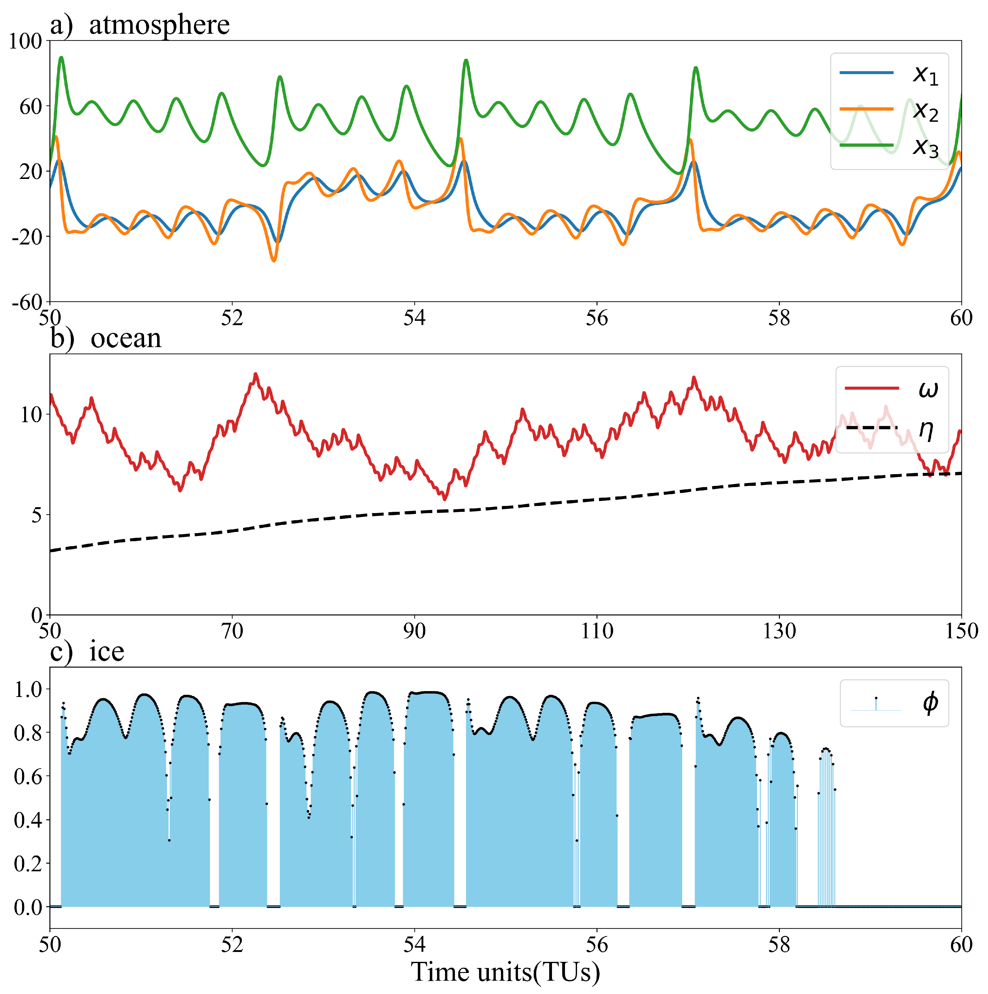
Referring to Han et al. (2013) [8], the parameter values of the true-value model are ( σ , κ , b, c 1 , c 2 , c 3 , c 4 , c 5 , c 6 , c 7 , c 8 , c 9 , c 10 , O m , O d , S m , S s , S p d , Γ , H i g , H i m , H 0 ) = (9.95, 28, 8/3, 0.1, 1, 0.01, 1, 0.01, 0.01, 0.01, 0.1, 0.1, 0.1, 10, 10, 10, 10, 1, 10, 10, 10, 10, 10, 10, 10, 10, 10, 10, 10, 100, 50, 10, 80). We integrated the model by using a fourth-order Runge-Kutta scheme, starting with the initial conditions ( x 1 , x 2 , x 3 , ω , η , φ ) = (0 , 1 , 0 , 0 , 0 , 0 , 0), and using the values after spin-up over 2500 TUs as the true initial values. Figure 2 shows the time series of the three atmospheric and two oceanic variables, as well as the sea-ice variable, and it can be observed that the three atmospheric variables have attractor characteristics. The x-axis of Figure 2 uses a different time scale, revealing that the variability of the oceanic variables is about 1/10 of that of the atmospheric variables.

3.2. Neural network model

We utilize background integration data to train a NN model aimed at establishing nonlinear relationships between atmospheric and oceanic variables.Specifically, for the coupled model employed in this study, we formulate the nonlinear relationship from the atmospheric variable X = [ x 1 , x 2 , x 3 ] to each of the oceanic and sea ice variables: ω , η , and φ .
Taking ω as an example, the objective of ML training is to construct a neural network G ˜ W to predict ω using the atmospheric variable x ( a ) , with W representing its weight. The optimal weights are determined through the minimization of the loss function during the training phase. To acquire the training data, we conduct a background integration of 5000 TUs for the model starting from a random initial value, with an integral step size of Δ t = 0.01 . This data is divided into 5000 TUs, comprising input-output pairs of atmospheric variables ( x 1 , 2 , 3 ) and oceanic variables ( ω ) at corresponding moments. Among these, 4000 TUs are allocated for model training, 800 TUs for validation and hyperparameter tuning during the training period, and the remaining 200 TUs are dedicated to evaluating the model’s robustness without any overlap among the three sequences.
Based on different assumptions, we constructed three DNN models as outlined below:
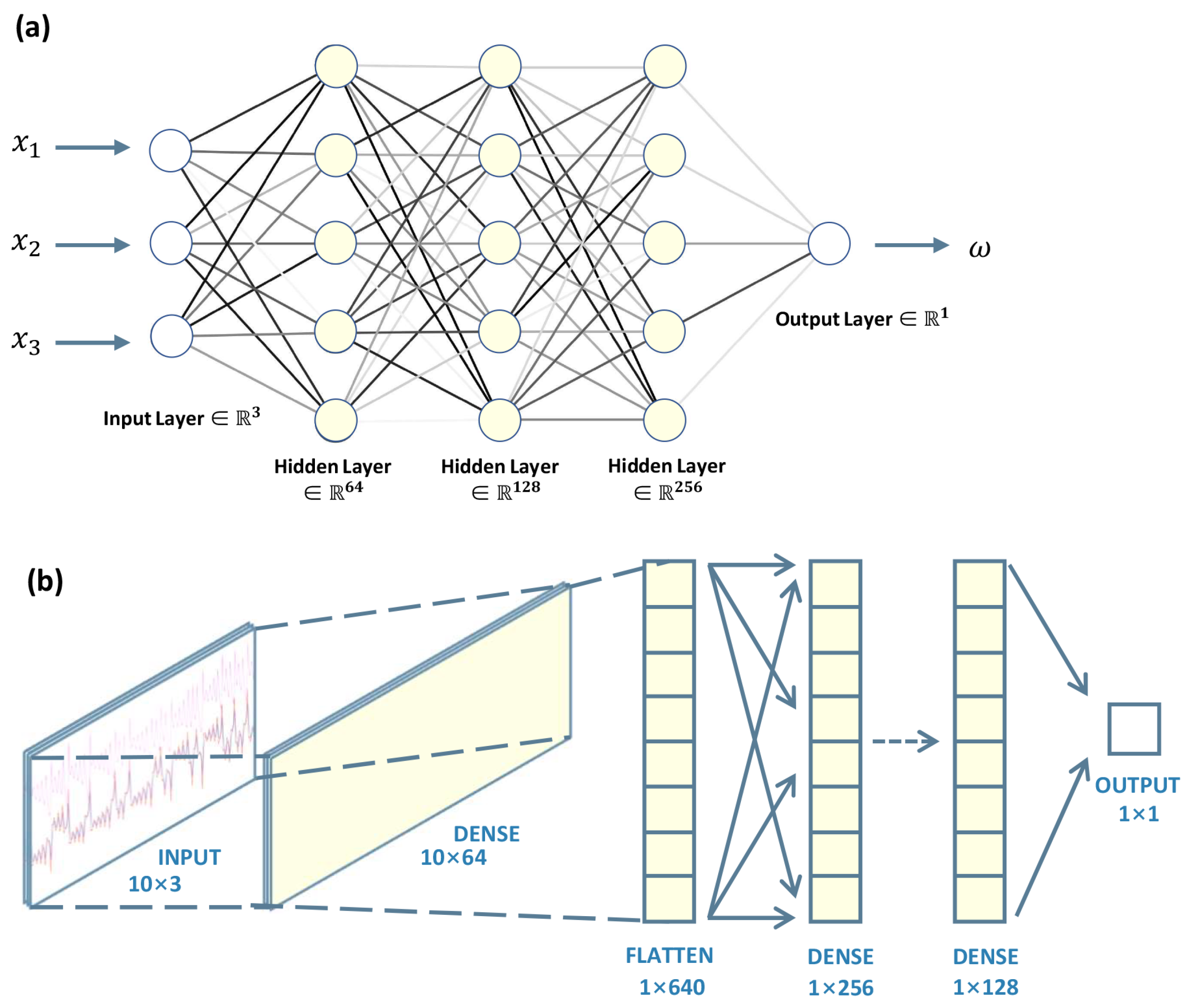
In the first model, we utilize atmospheric variables to predict concurrent oceanic variables, naming this model the Single-Instant Predictor (SIP). The training involves a three-layer fully connected network model; refer to Figure 3a for the schematic neural network structure. The training objective is to achieve the desired nonlinear model, expressed as ω ( t ) = G ˜ X ( t ) .
In accordance with findings by Lu et al. (2015), indicating that utilizing atmospheric observations with lead times can significantly enhance analysis quality in WCDA compared to SCDA using a small ensemble size [11], our second model associates the oceanic variables with the previous atmospheric variables. Specifically, we construct the model to predict the current oceanic variable using the atmospheric variable 0.2 TUs ahead of time. We term this model a Single-Step Leading Predictor (SLP). The network is the same as SIP, also refer to Figure 3a, and the training results in a target nonlinear model expressed as ω ( t ) = G ˜ X ( t 0.2 ) .
Building on Lu et al. (2015) strategy of averaging time-leading atmospheric variables to construct ocean-atmosphere covariance, which reduces noise arising from disparate variability in the atmosphere and ocean, our third model utilizes all atmospheric variables from the 10 consecutive steps to predict ocean variables in the final step. Termed the Multi-Leading Predictor (MLP), the network model is depicted in Figure 3b, trained to achieve the target nonlinear model ω ( t ) = G ˜ X ( t 9 , t ) . Importantly, the inputs in each data pair include atmospheric variables from the 10-step model integration, while the outputs represent oceanic variables from the final step. Consequently, the volume of data for both training and validation is only 1/10th of that used for the first two models.
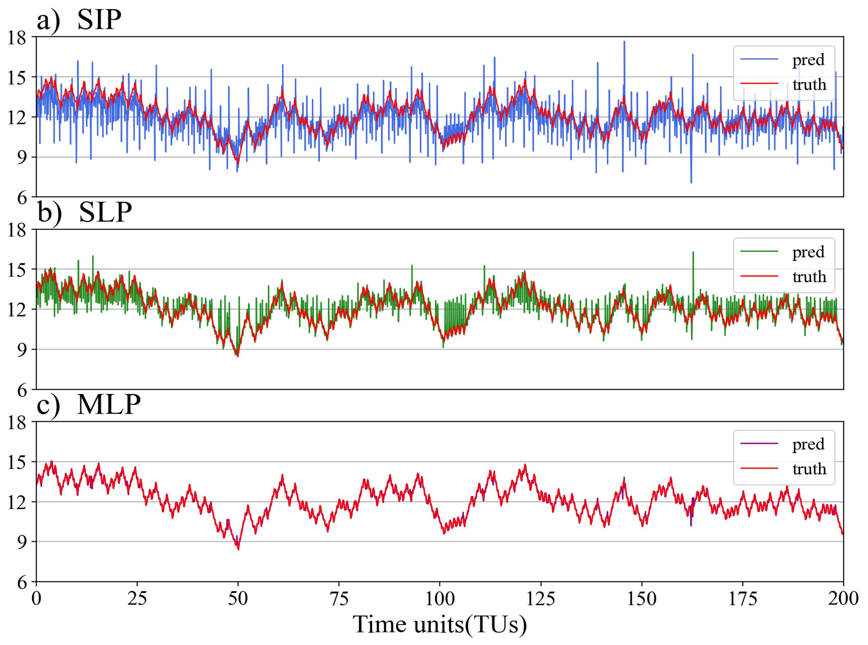
We use the three aforementioned models to establish the relationship between X and ω , the models’ parameters are optimized using the Adam algorithm and the loss function is the Huber loss over the training dataset, made of background snapshots. The training consists of 200 epochs with an adaptive learning rate (initial learning rate sets 1 10 3 ) and batch size of 50. After the entire training step, we keep the model which yields the lowest loss over the validation dataset. The three aforementioned models to establish the relationship between X and ω , the stabilized prediction results are shown in Figure 4. Figure 4a, b,c illustrate the performances of the three models on the same test set, where the red line represents the true value, while the blue, green, and violet lines correspond to the predicted ω -values by the three models, respectively. It can be observed that all three models can roughly simulate the trend of the true value, and for the SIP, some extreme values appear due to the large variability difference between the atmospheric and oceanic variables; the stability of the SLP (b) is significantly improved compared to (a); and the MLP (c) achieves a more satisfactory prediction result. This also indicates that the use of training data related to the leading-averaged atmospheric variables enhances the accuracy of sea-air predictions.
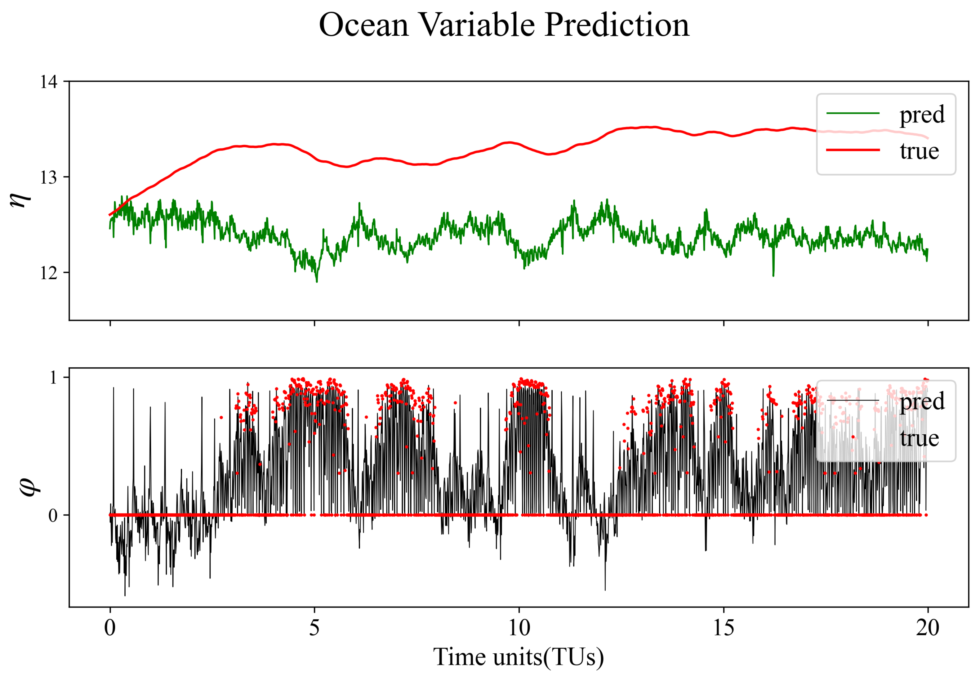
We have employed a similar approach to train the relationship between X and the deep-ocean pycnocline variable η , as well as the sea ice variable φ with MLP, as shown in Figure 5. The results show that the relationship between the fast-varying atmospheric variables and the slow-varying pycnocline variables is notably weak, making the prediction of η with the atmosphere nearly impossible. On the other hand, the prediction of sea ice with atmospheric variables proves to be difficult. This discrepancy can be attributed to the relatively weak connection between these variables in the model equations. We therefore focus on the SCDA of atmospheric observations to the sea surface variable ω in the assimilation experiments below, which is also consistent with the idea of interface decomposition proposed by [13].

3.3. Data assimilation experiment settings

The true values and observations used as reference are generated by integrating the coupled model with standard parameter values (cf. Section 3.1). The integration begins with the true initial values obtained in Section 3.1, and the model integration step is Δ t = 0.01 TUs, spanning a total of 100 TUs for the entire experiment. Observational data are generated by adding random noise, following a specific distribution, to the true values. To simulate real-world conditions, we assume that atmospheric, sea surface, and sea ice variables can be observed at specific time intervals, whereas the pycnocline variable η is unobservable. Following the setup of Zhang [32], we assume that observation errors for the atmospheric variables x 1 , 2 , 3 all follow a Gaussian distribution with a standard deviation of 2. The observation errors for ω and φ are assumed to follow Gaussian distributions with standard deviations of 0.5 and 0.1, respectively. Additionally, to simulate mode errors, we introduce biased coupled modes in both the background integration and assimilation experiments. Here, all physical parameters are perturbed from the reference parameters with a 1% random error.
Assimilation experiments were conducted to compare the performance of conventional EAKF and DNN-EAKF in SCDA. Prior studies indicate that high-frequency atmospheric observations positively impact oceanic variables, while low-frequency oceanic observations struggle to adjust atmospheric variables [8,10]. Hence, our emphasis is on evaluating SCDA concerning atmospheric observations, while using WCDA to assimilate ocean and sea ice observations. Three CDA frameworks can be established for atmospheric observations: WCDA, SCDA at the interface (SCDA-I), and fully SCDA (SCDA-F). The influence of observations on various variables is illustrated in Figure 6. Among them, SCDA-I utilizes atmospheric observations to update the sea surface variable ω , which references [13].
As shown in Figure 4, a DNN can efficiently establish a nonlinear relationship between atmospheric variables x 1 , 2 , 3 and the sea surface variable ω . However, establishing a relationship between atmospheric variables and pycnocline or sea ice variables remains challenging (Figure 5). Therefore, we employ DNN-EAKF to update ω using atmospheric observations in SCDA-I (black box in Figure 6b). We then compare the results with those of the three CDA experiments using the conventional EAKF method.
In the subsequent discussion, we initially present the results of assimilating only atmospheric observations and subsequently extend our analysis to encompass the assimilation of all available observations.

4. Results

4.1. Atmosphere observations

In the initial scenario, the focus is on assimilating exclusively atmospheric observations into the coupled model, employing various CDA frameworks and methodologies. Various assimilation intervals (e.g., assimilating atmospheric observations every 0.1 or 0.2 TUs) and multiple ensemble sizes (with N representing the ensemble member size, ranging from 10 to 50) are explored. The assessment of data assimilation results includes comparing true values using metrics such as root-mean-squared errors (RMSEs) and anomaly correlation coefficient (ACC). In this context, RMSE and ACC are defined as:
RMSE = 1 K i = 1 K x i a ¯ x i true 2
and
ACC = 1 K 1 i = 1 K x i a ¯ x a ¯ x i t r u e ¯ x t r u e ¯ 1 K 1 i = 1 K x i a ¯ x a ¯ 2 1 K 1 i = 1 K x i t r u e ¯ x t r u e ¯ 2
In these equations, K denotes the time steps for a state variable x, while x a ¯ and x true signify the ensemble mean of the analysis and true values of variable x, respectively. To ensure the reliability of the conclusions, we utilized the results from the last 30 TUs for calculating RMSE and ACC.
To mitigate the impact of randomness in the outcomes, each experiment was replicated 10 times with different initial perturbation values. The final results were determined based on the mean values of RMSE and ACC obtained from these ten experiments.
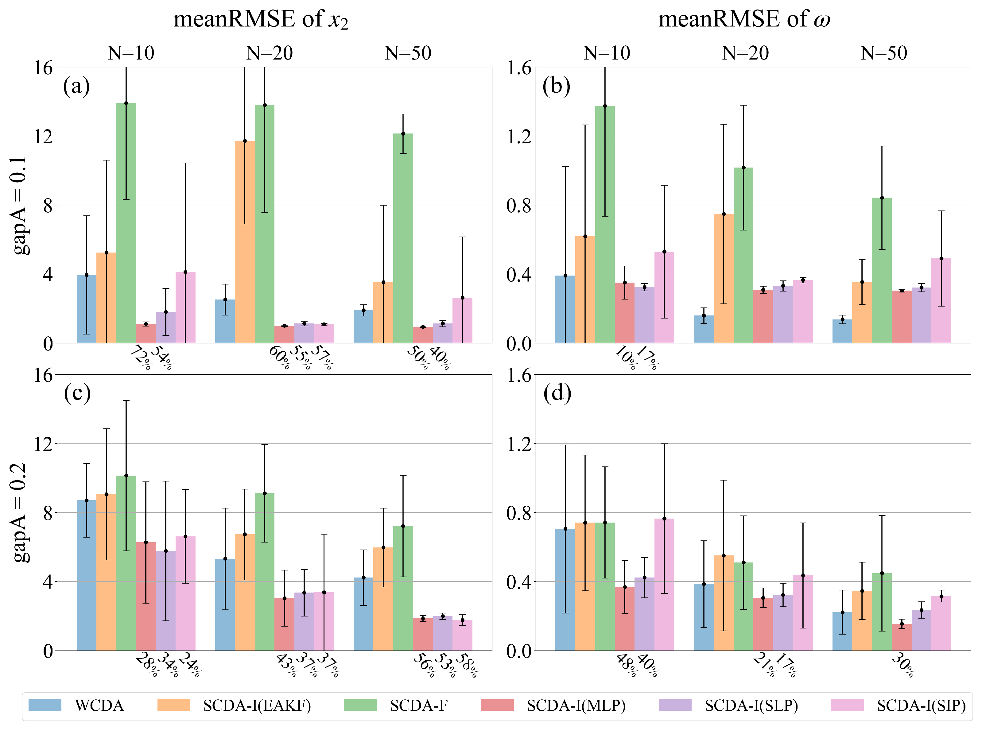
In this scenario, we examine the outcomes related to the atmospheric variable x 2 and the oceanic variable ω . Figure 7 depicts histograms illustrating the RMSE distributions for each method. The bar values denote the mean of 10 replicate experiments, and the error bars indicate their standard deviation.
Comparing RMSE, it is evident that, in the realm of CDA utilizing EAKF, SCDA-F (green) exhibits poor performance, while WCDA (blue) demonstrates superior performance. Additionally, their assimilation effectiveness improves with larger ensemble sizes and more frequent observations. This indicates that introducing cross-component error covariance through linear approximation may degrade state estimation when there are insufficient ensemble members, consistent with findings in [8]. The detrimental impact of an increased frequency of atmospheric observations on the assimilation performance of SCDA-F (green) is conspicuous. This implies that poorly estimated cross-component error covariances can accumulate adverse effects when rapidly incorporating atmospheric observation information.
Regarding the ocean variable ω in Figure 7b and 7d, DNN-EAKF consistently outperforms the conventional EAKF approach in SCDA-I (orange). This indicates that, even with smaller ensembles, atmospheric observations can accurately adjust ocean variables through nonlinear mapping, thanks to the enhanced signal-to-noise ratio of the cross-component error covariance. In line with the diverse behaviors of different models illustrated in Figure 4, SCDA-I(MLP) (red), exhibiting the highest prediction accuracy, performs optimally in most cases. However, the large standard deviation of the results from the 10 replicate experiments reveals that the predictive effect of SCDA-I(SIP) (pink) is not sufficiently stable, limiting the method’s performance.
Additionally, it is observed that SCDA-I using DNN-EAKF surpasses the assimilation effect of WCDA in some instances, particularly with an observation interval of 0.2 TUs. This implies a positive updating effect of atmospheric observations on oceanic variables through DNN-EAKF. We define the relative error reduction rate r as
r = R M S E ¯ W C D A R M S E ¯ D N N E A K F R M S E ¯ W C D A ,
denoting the relative error reduction of SCDA-I using DNN-EAKF compared to WCDA and representing the improvement effect from the cross-component update based on DNN-EAKF. The value of r is indicated in Figure 7 beneath the bar where SCDA-I using DNNs outperforms WCDA. It highlights that the error reduction of DNN-EAKF over WCDA becomes more prominent with an extended atmospheric observation interval and a smaller ensemble size. This signifies situations where DNN-EAKF holds a more significant advantage, namely when the problem is more nonlinear, and the ensemble size is limited.
Figure 7c shows a notable increase in the relative error reduction rate for the atmospheric variables with an expanding ensemble when the observation interval is 0.2TUs. This is attributed to the substantial improvement that DNN-EAKF brings to the oceanic variables in this scenario, resulting in a decrease in oceanic error with the increasing ensemble size. It can be inferred that the coupling with the improved ω contributes to improving the accuracy of x 2 in SCDA-I using DNN-EAKF.
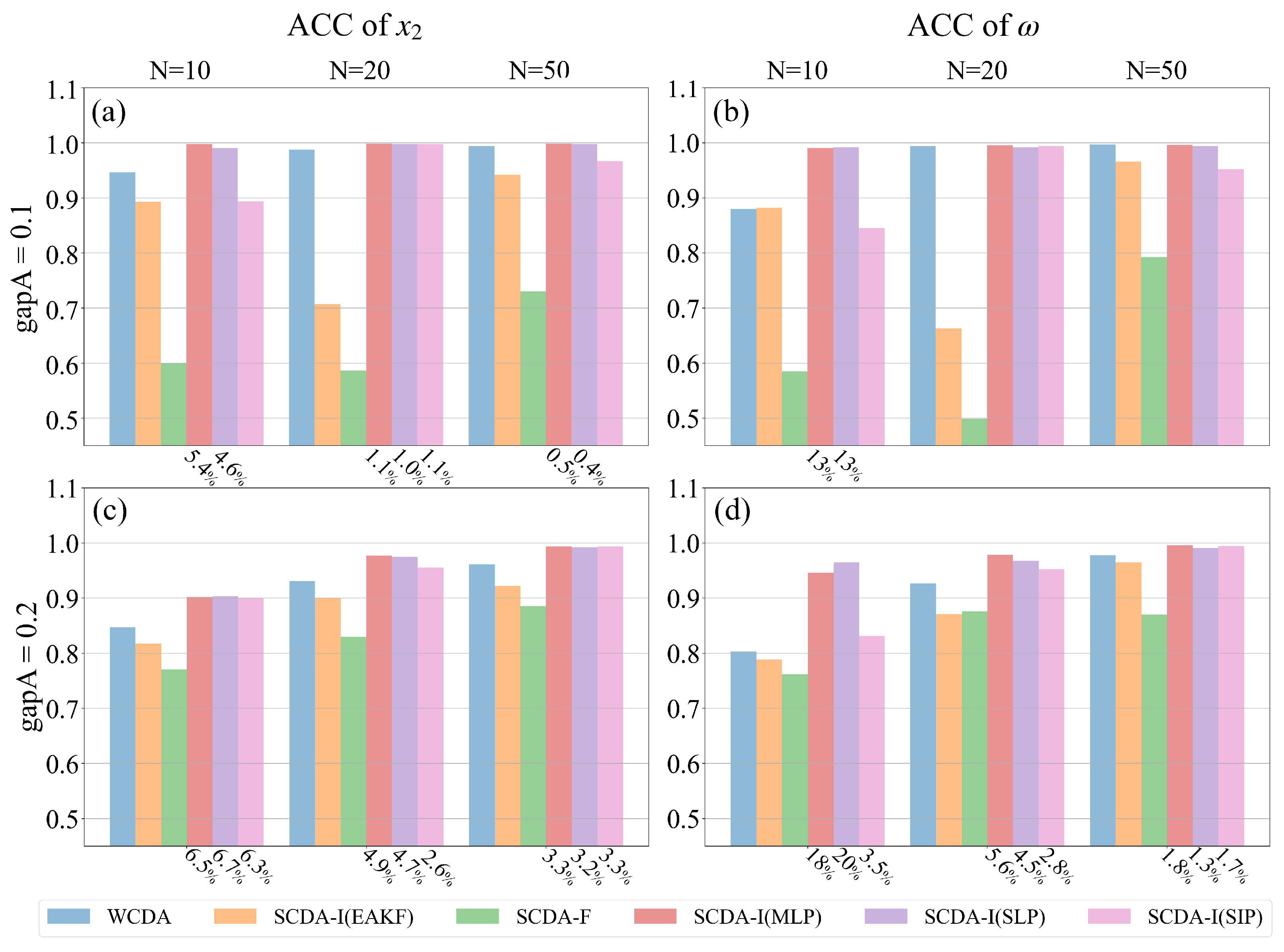
Figure 8 displays the ACC corresponding to the results shown in Figure 7, reaffirming the same conclusion. It should be noted that the ratio labeled is the ACC growth instead of RMSE reduction. Clearly, SCDA-I based on DNN-EAKF, especially when utilizing the MLP model, consistently produces significantly enhanced assimilation results compared to WCDA. The advantage is more pronounced in scenarios characterized by stronger nonlinearity and smaller ensemble sizes.
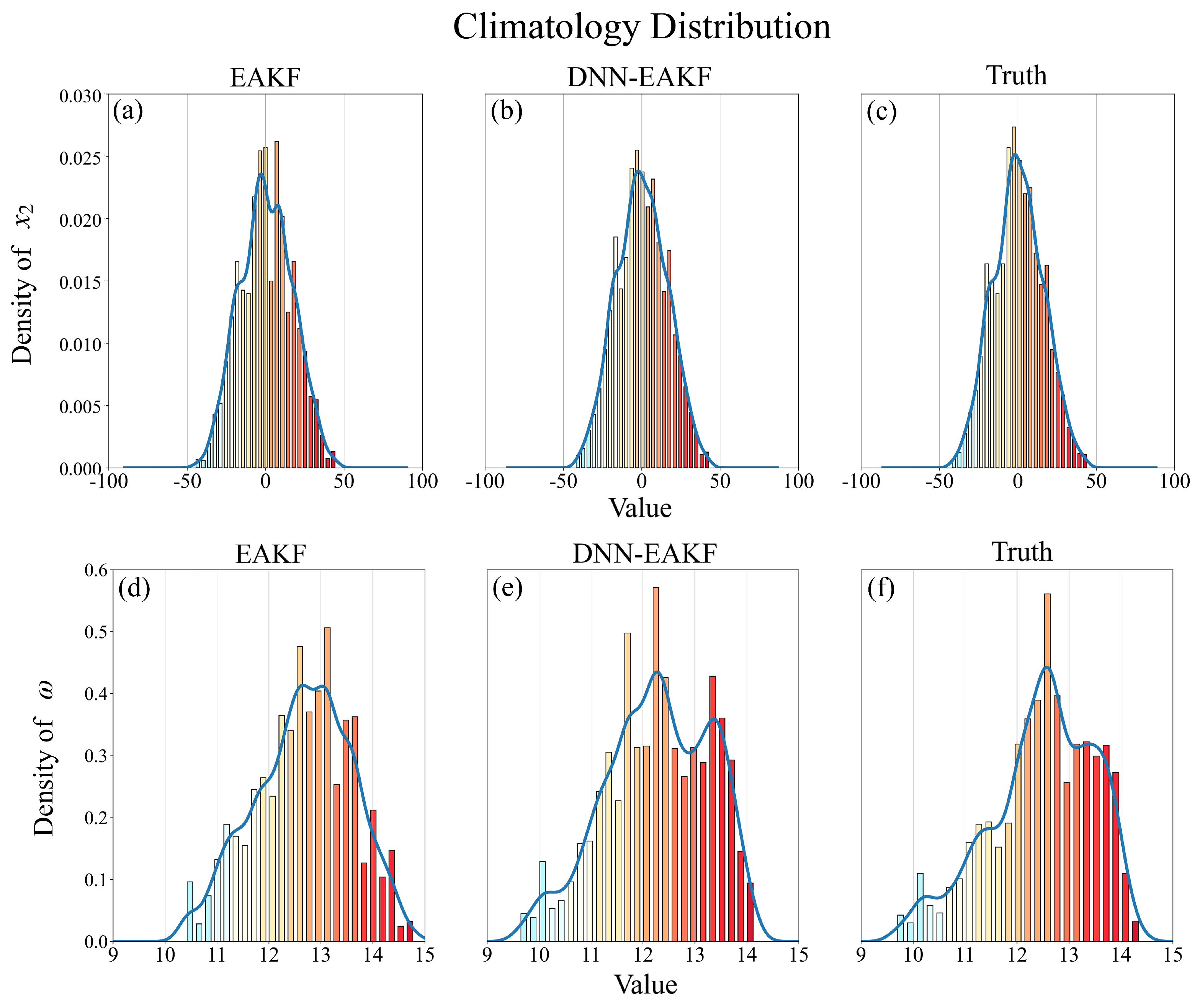
It is intriguing to further investigate how DNN-EAKF addresses nonlinearities. Figure 9 illustrates the probability distributions of x 2 and ω (i.e., climatological state distributions) in the mean of analysis field using 50 ensemble members at an observation interval of 0.2 TUs. Once again, we rely on the results from the last 30 TUs and compare the climatological distributions of WCDA, SCDA-I (MLP), and the true values. Notably, the climatological distributions of the atmospheric variables do not differ significantly between the three methods. However, for the oceanic variables, the climatological distributions of the true values exhibit a non-Gaussian pattern, featuring two local maxima (or "peaks") around ω = 13.5 and ω = 10 . While the climatological distributions of the EAKF results inadequately capture these probability peaks, those of the DNN-EAKF align more closely with the distributions of the true values, providing a better match.
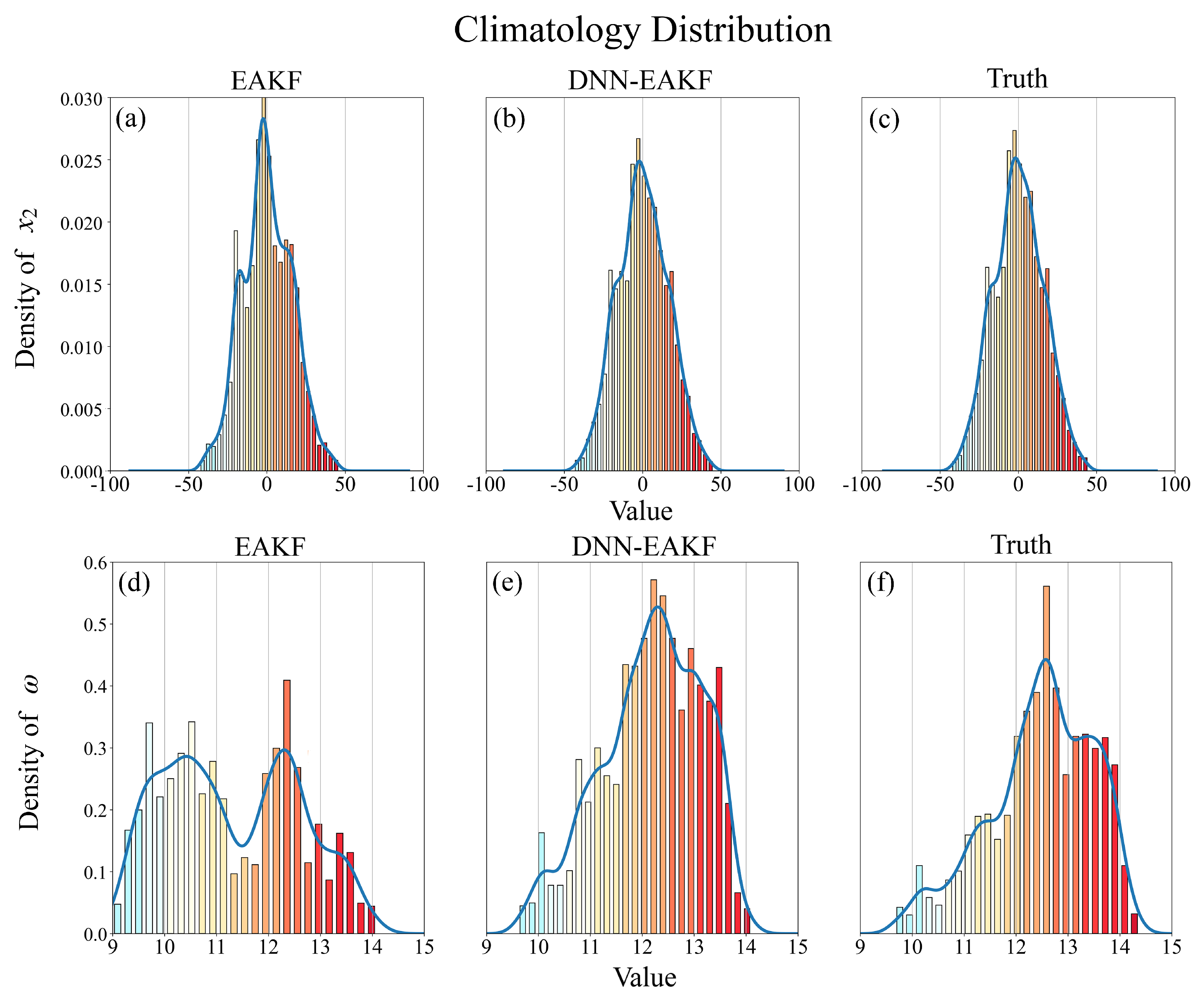
Remarkably, even with a reduced number of ensemble members, e.g., N = 10, the DNN-EAKF results characterise the ocean climatology well (Figure 10e,f), whereas the climatology of the conventional EAKF results differ significantly from that of the true values (Figure 10d,f). This observation suggests that the method excels in handling nonlinear problems, shedding light on the underlying reasons for its advantages.

4.2. Full observations

Experiments in Section 4.1, exclusively assimilating atmospheric observations, demonstrated that SCDA-I using DNN-EAKF effectively improves cross-component updates. It results in a more stable and accurate model state compared to EAKF, particularly in conditions with pronounced nonlinearities, such as those with low assimilation frequencies and few ensemble members. In this section, we investigate the broader impact of DNN-EAKF on the overall variables of the coupled model, considering multiple observations, including atmosphere, sea surface, and sea ice. A more realistic scenario is considered, where oceanic observations are less frequent than those for the atmosphere. Specifically, we assume an observation interval of 0.1 TUs for the atmosphere and 0.5 TUs for the oceans and sea ice. This results in atmospheric observations directly updating ocean variables more frequently than oceanic observations in SCDA-F and SCDA-I. However, inaccurate cross-component error covariances can significantly degrade assimilation results compared to WCDA.
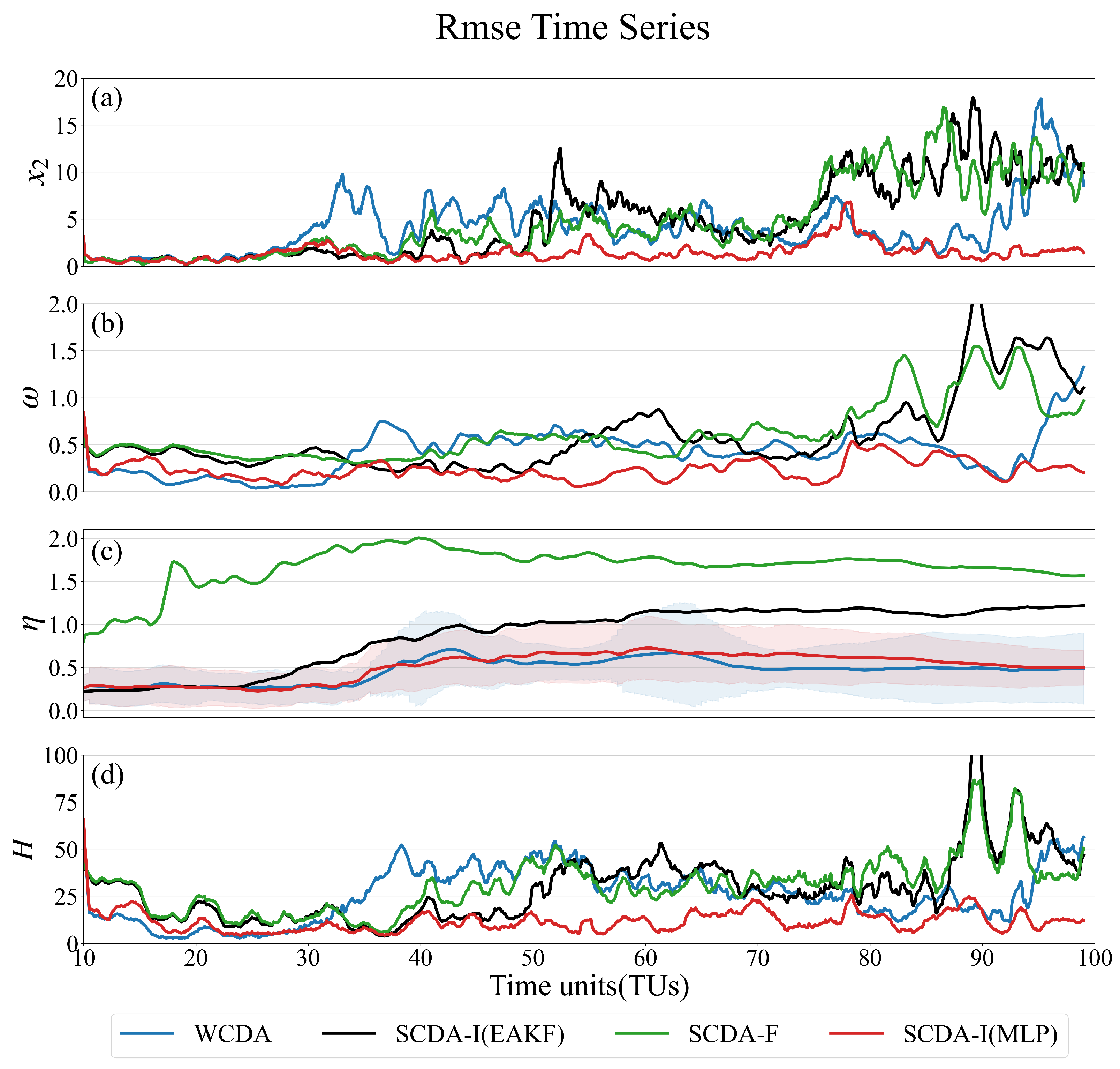
We calculate the RMSE at each step using the experimental results of the 10 ensemble members compared to the true values and present them in Figure 11, focusing on the impact of SCDA-I (MLP).To mitigate randomness, we computed the average RMSE over 10 repeated experiments. For the purpose of presentation, we applied a smoothing process to the time series of RMSE, using a moving average with a window size of 1TU (or 100 steps). Consistent with findings from experiments assimilating only atmospheric observations, SCDA-I (MLP) effectively assimilates both x 2 and ω , surpassing the performance of the three coupled assimilation frameworks using the conventional EAKF. While SCDA-F’s influence on the assimilation of these two variables is weaker than that of WCDA and SCDA-I, it remains within an acceptable range due to the presence of ocean observations constraining the ocean variables. The enhancements in ocean variable assimilation achieved by SCDA-I are also manifested in η and φ (Figure 11 shows the corresponding enthalpies H), indicating improved assimilation results for the deep-sea and sea ice.
For more detailed quantitative results, Table 1 presents the time-averaged RMSEs of x 2 , ω , η and φ from the experimental results with varying ensemble sizes. In these experiments, the SCDA-I experiments used the conventional EAKF and three DNN models. Examination of the data reveals clear advantages of DNN-EAKF, including reduced analysis errors and improved ACC. Notably, among the three DNN models, SLP performs best for atmospheric variables, while MLP excels for ocean and related variables. Table 1 also illustrates the relative error reduction rate and relative ACC increase rate of SCDA-I (MLP) compared to WCDA. The improvement resulting from strongly coupled data assimilation is particularly pronounced with a smaller number of ensemble members.

5. Conclusion

In recent years, the research of CDA has received extensive attention, among which SCDA is considered the theoretically optimal coupled data assimilation method for reanalysis and prediction initialization. And one of the key challenges of SCDA is to accurately estimate its coupled error covariance matrix, especially the cross-component error covariance. Numerous studies have shown that in ensemble-based assimilation algorithms, the accuracy of covariance estimation is largely contingent on the ensemble size.
In order to solve the difficulties faced by EnKF in SCDA, this paper proposes a Deep Neural Network-Ensemble Kalman Filtering algorithm (DNN-EAKF), which incorporates machine learning on the basis of EAKF for improvement. In this study, the assimilation performance of the algorithm is verified using a conceptual coupled model, and the results show that DNN-EAKF utilizes a nonlinear model instead of the local linear mapping of EAKF, which makes the state values more stable and improves the estimation accuracy to some extent. It is further found that, consistent with the results in Han et al. (2013)[8], atmospheric observations can improve the ocean state by providing accurate coupled covariances, and DNN-EAKF generates robust cross-component error covariances even when dealing with limited ensemble members, which mitigates the need for huge computational costs to some extent, effectively conveying atmospheric observation information to the constituent variables through coupling. Numerical results from a series of experiments under different assumptions show that DNN-EAKF performs comparable or even better performance than the EAKF sequential assimilation algorithm using finite ensemble statistics while requiring fewer computational resources (ensemble members and observations).
This study primarily presents the rationale behind the DNN-EAKF algorithm and validates the concept using a relatively low-order model. While the simple model demonstrates promising results, various challenges persist in its application to realistic high-resolution models. Specifically, the computational cost of training the machine learning model escalates in complicated coupled models, and predictions generated during assimilation by the machine learning model introduce computational overhead. Moreover, its superiority over EAKF in weak non-linearity cases is not significant. In future research, our focus will be on further optimizing DNN-EAKF in additional low-order models and its application to real operational prediction models.

Author Contributions

Conceptualization, Z.S; methodology, R.W. and Z.S.; software, R.W. and Z.S.; validation, R.W.; writing—original draft preparation, R.W.; writing—review and editing, Z.S.; visualization, R.W.; supervision, Z.S.; project administration, Z.S.; funding acquisition, Z.S. All authors have read and agreed to the published version of the manuscript.

Funding

This study was supported by grants from the National Natural Science Foundation of China (42176003), the Jiangsu Provincial Innovation and Entrepreneurship Doctor Program (JSSCBS20210252)

Data Availability Statement

The original contributions presented in the study are included in the article, further inquiries can be directed to the corresponding author.

Conflicts of Interest

The authors declare no conflict of interest.

References

  1. Fujii, Y.; Nakaegawa, T.; Matsumoto, S.; Yasuda, T.; Yamanaka, G.; Kamachi, M. Coupled climate simulation by constraining ocean fields in a coupled model with ocean data. Journal of Climate 2009, 22, 5541–5557. [Google Scholar] [CrossRef]
  2. Saha, S.; Nadiga, S.; Thiaw, C.; Wang, J.; Wang, W.; Zhang, Q.; Van den Dool, H.; Pan, H.L.; Moorthi, S.; Behringer, D. others. The NCEP climate forecast system. Journal of Climate 2006, 19, 3483–3517. [Google Scholar] [CrossRef]
  3. Anderson, J.L. An ensemble adjustment Kalman filter for data assimilation. Monthly weather review 2001, 129, 2884–2903. [Google Scholar] [CrossRef]
  4. Zhang, R.; Delworth, T.L. Impact of the Atlantic multidecadal oscillation on North Pacific climate variability. Geophysical Research Letters 2007, 34. [Google Scholar] [CrossRef]
  5. Zhang, S. A Study of Impacts of Coupled Model Initial Shocks and State–Parameter Optimization on Climate Predictions Using a Simple Pycnocline Prediction Model. Journal of Climate 2011, 24, 6210–6226. [Google Scholar] [CrossRef]
  6. Zhang, S.; Liu, Z.; Zhang, X.; Wu, X.; Deng, X. Coupled data assimilation and parameter estimation in coupled ocean–atmosphere models: a review. Climate Dynamics 2020, 54. [Google Scholar] [CrossRef]
  7. Penny, S.G.; Bach, E.; Bhargava, K.; Chang, C.; Da, C.; Sun, L.; Yoshida, T. Strongly Coupled Data Assimilation in Multiscale Media: Experiments Using a Quasi-Geostrophic Coupled Model. 2019; 11, 1803–1829. [Google Scholar] [CrossRef]
  8. Han, G.; Wu, X.; Zhang, S.; Liu, Z.; Li, W. Error covariance estimation for coupled data assimilation using a Lorenz atmosphere and a simple pycnocline ocean model. Journal of Climate 2013, 26, 10218–10231. [Google Scholar] [CrossRef]
  9. Liu, Z.; Wu, S.; Zhang, S.; Liu, Y.; Rong, X. Ensemble data assimilation in a simple coupled climate model: The role of ocean-atmosphere interaction. Advances in Atmospheric Sciences 2013, 30, 1235–1248. [Google Scholar] [CrossRef]
  10. Sluka, T.; Penny, S.; Kalnay, E.; Miyoshi, T. Strongly coupled enkf data assimilation in coupled ocean-atmosphere models. The 96th AMS Annual Meeting,“Earth System Science in Service to Society. 2016; 10–14. [Google Scholar]
  11. Lu, F.; Liu, Z.; Zhang, S.; Liu, Y. Strongly coupled data assimilation using leading averaged coupled covariance (LACC). Part I: Simple model study. Monthly Weather Review 2015, 143, 3823–3837. [Google Scholar] [CrossRef]
  12. Smith, P.J.; Lawless, A.S.; Nichols, N.K. Treating sample covariances for use in strongly coupled atmosphere-ocean data assimilation. Geophysical Research Letters 2018, 45, 445–454. [Google Scholar] [CrossRef]
  13. Frolov, S.; Bishop, C.H.; Holt, T.; Cummings, J.; Kuhl, D. Facilitating strongly coupled ocean–atmosphere data assimilation with an interface solver. Monthly Weather Review 2016, 144, 3–20. [Google Scholar] [CrossRef]
  14. Yoshida, T. Covariance localization in strongly coupled data assimilation. PhD thesis, University of Maryland, College Park, 2019. [Google Scholar]
  15. Shen, Z.; Tang, Y.; Li, X.; Gao, Y. On the Localization in Strongly Coupled Ensemble Data Assimilation Using a Two-Scale Lorenz Model. Earth and Space Science 2021, 8, e2020EA001465. [Google Scholar] [CrossRef]
  16. Cheng, S.; Quilodrán-Casas, C.; Ouala, S.; Farchi, A.; Liu, C.; Tandeo, P.; Fablet, R.; Lucor, D.; Iooss, B.; Brajard, J.; Xiao, D.; Janjic, T.; Ding, W.; Guo, Y.; Carrassi, A.; Bocquet, M.; Arcucci, R. Machine Learning With Data Assimilation and Uncertainty Quantification for Dynamical Systems: A Review. IEEE/CAA Journal of Automatica Sinica 2023, 10, 1361–1387. [Google Scholar] [CrossRef]
  17. Arcucci, R.; Zhu, J.; Hu, S.; Guo, Y.K. Deep data assimilation: integrating deep learning with data assimilation. Applied Sciences 2021, 11, 1114. [Google Scholar] [CrossRef]
  18. Farchi, A.; Bocquet, M.; Laloyaux, P.; Bonavita, M.; Malartic, Q. A comparison of combined data assimilation and machine learning methods for offline and online model error correction. Journal of computational science 2021, 55, 101468. [Google Scholar] [CrossRef]
  19. Li, X.; Xiao, C.; Cheng, A.; Lin, H. Joint estimation of parameter and state with hybrid data assimilation and machine learning. 2022. [Google Scholar]
  20. Legler, S.; Janjić, T. Combining data assimilation and machine learning to estimate parameters of a convective-scale model. Quarterly Journal of the Royal Meteorological Society 2022, 148, 860–874. [Google Scholar] [CrossRef]
  21. Brajard, J.; Carrassi, A.; Bocquet, M.; Bertino, L. Combining data assimilation and machine learning to emulate a dynamical model from sparse and noisy observations: A case study with the Lorenz 96 model. Journal of computational science 2020, 44, 101171. [Google Scholar] [CrossRef]
  22. Vlachas, P.R.; Byeon, W.; Wan, Z.Y.; Sapsis, T.P.; Koumoutsakos, P. Data-driven forecasting of high-dimensional chaotic systems with long short-term memory networks. Proceedings of the Royal Society A: Mathematical, Physical and Engineering Sciences 2018, 474, 20170844. [Google Scholar] [CrossRef] [PubMed]
  23. Bocquet, M.; Brajard, J.; Carrassi, A.; Bertino, L. Data assimilation as a learning tool to infer ordinary differential equation representations of dynamical models. Nonlinear Processes in Geophysics 2019, 26, 143–162. [Google Scholar] [CrossRef]
  24. Evensen, G. Sequential data assimilation with a nonlinear quasi-geostrophic model using Monte Carlo methods to forecast error statistics. Journal of Geophysical Research: Oceans 1994, 99, 10143–10162. [Google Scholar] [CrossRef]
  25. Kalman, R.E. A new approach to linear filtering and prediction problems. Journal of basic Engineering 1960, 82, 35–45. [Google Scholar] [CrossRef]
  26. Luo, X.; Hoteit, I. Ensemble Kalman filtering with a divided state-space strategy for coupled data assimilation problems. Monthly Weather Review 2014, 142, 4542–4558. [Google Scholar] [CrossRef]
  27. Whitaker, J.S.; Hamill, T.M. Ensemble data assimilation without perturbed observations. Monthly weather review 2002, 130, 1913–1924. [Google Scholar] [CrossRef]
  28. Bishop, C.H.; Etherton, B.J.; Majumdar, S.J. Adaptive sampling with the ensemble transform Kalman filter. Part I: Theoretical aspects. Monthly weather review 2001, 129, 420–436. [Google Scholar] [CrossRef]
  29. Anderson, J.L. A local least squares framework for ensemble filtering. Monthly Weather Review 2003, 131, 634–642. [Google Scholar] [CrossRef]
  30. Han, G.J.; Zhang, X.F.; Zhang, S.; Wu, X.R.; Liu, Z. Mitigation of coupled model biases induced by dynamical core misfitting through parameter optimization: simulation with a simple pycnocline prediction model. Nonlinear Processes in Geophysics 2014, 21, 357–366. [Google Scholar] [CrossRef]
  31. Zhang, S. A study of impacts of coupled model initial shocks and state–parameter optimization on climate predictions using a simple pycnocline prediction model. Journal of Climate 2011, 24, 6210–6226. [Google Scholar] [CrossRef]
  32. Zhang, S. Impact of observation-optimized model parameters on decadal predictions: Simulation with a simple pycnocline prediction model. Geophysical Research Letters 2011, 38. [Google Scholar] [CrossRef]
  33. Zhang, S.; Liu, Z.; Rosati, A.; Delworth, T. A study of enhancive parameter correction with coupled data assimilation for climate estimation and prediction using a simple coupled model. Tellus A: Dynamic Meteorology and Oceanography 2012, 64, 10963. [Google Scholar] [CrossRef]
  34. Zhang, S.; Winton, M.; Rosati, A.; Delworth, T.; Huang, B. Impact of enthalpy-based ensemble filtering sea ice data assimilation on decadal predictions: Simulation with a conceptual pycnocline prediction model. Journal of climate 2013, 26, 2368–2378. [Google Scholar] [CrossRef]
  35. Lorenz, E.N. Deterministic nonperiodic flow. Journal of atmospheric sciences 1963, 20, 130–141. [Google Scholar] [CrossRef]
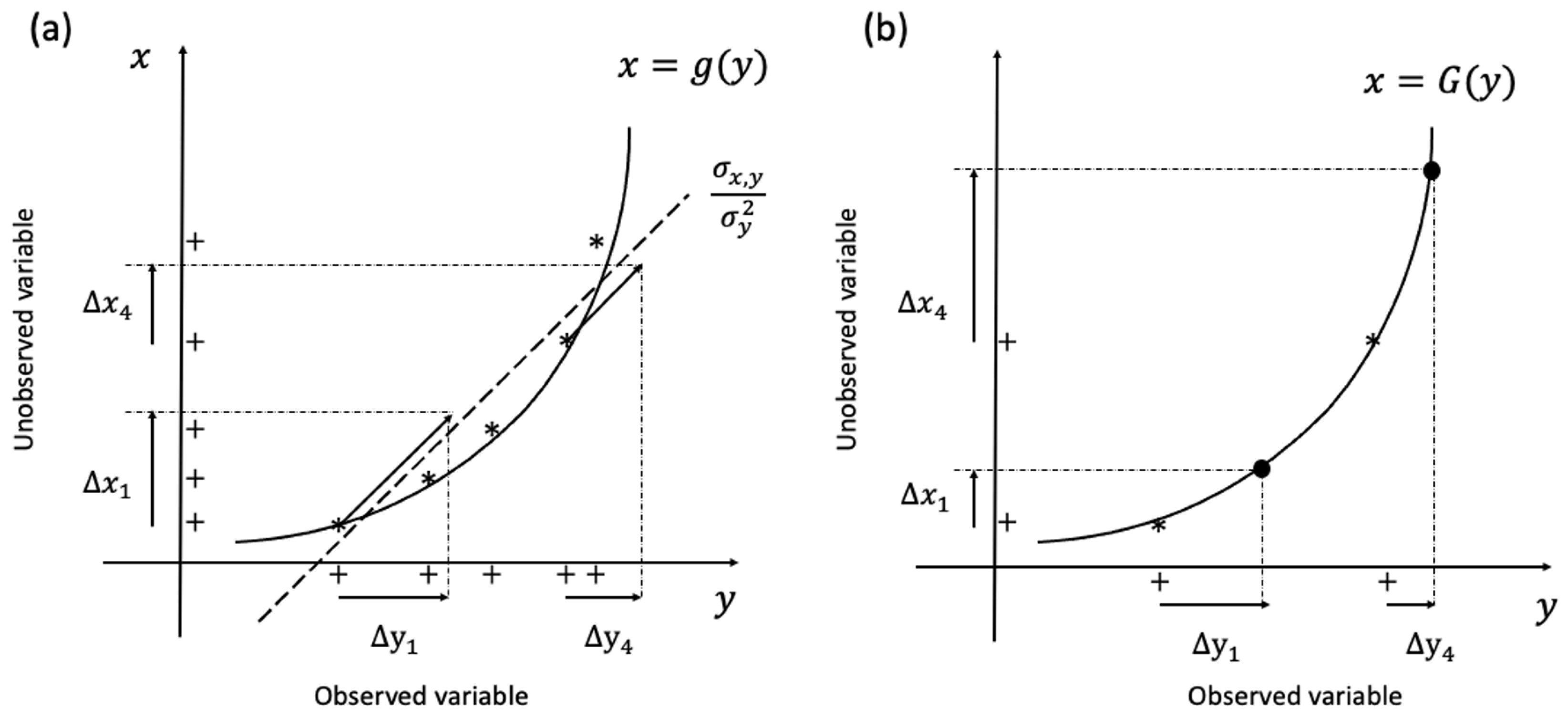
Figure 1. Schematic diagram of the state variable update algorithm in EAKF (a) and DNN-EAKF (b), where g or G is the nonlinear relationship between the observed variable y and the unobserved variable x, with "*" representing ensemble members and "+" representing the projection of ensemble members on the x / y axis.
Preprints 92247 g001
Figure 2. The variability of the atmosphere (a); ocean (b); and sea ice (c) variables.
Preprints 92247 g002
Figure 3. Schematic diagram of the neural networks. (a) A three-layer fully connected neural network for two single-step prediction models with input and output sizes of 3 and 1, respectively; (b) A fully connected neural network for a multi-step prediction model with input and output sizes of [10,3] and 1, respectively.
Preprints 92247 g003
Figure 4. Prediction effects of Single-instant Predictor (a), Single-leading Predictor (b) and Multi-leading Predictor (c) on the test set .
Preprints 92247 g004
Figure 5. MLP model for η (a) and ϕ (b).
Preprints 92247 g005
Figure 6. Three frameworks for coupling assimilation. The horizontal axis represents the observed variables, and the vertical axis represents the variables affected by each observation. The dark gray shadows in SCDA-I(b) represent the DNN-EAKF method obtained using conventional EAKF or DNN-based training models in the atmospheric observation effect ω variable.
Preprints 92247 g006
Figure 7. The time averaged RMSEs of WCDA (blue), SCDA-I(EAKF) (orange), SCDA-F (green), SCDA-I(MLP) (red), SCDA-I(SLP) (violet), and SCDA-I(SIP) (pink) for the atmospheric variable x 2 when the atmospheric observation interval is 0.1TUs(a) and 0.2TUs(c), within the [70,100] TUs timeframe; (b)(d) same as (a)(c), but for the ocean variable ω . The error bars represent the standard deviation of the RMSE of 10 replicate experiments for each coupled method; the ratios beneath the bar of DNN-EAKF are the error reduction rates compared to WCDA (blue).
Preprints 92247 g007
Figure 8. Same as Figure 7, but for the ACC. Accordingly, the ratio r labeled there is the DNN-EAKF ACC value growth rate compared to WCDA (blue).
Preprints 92247 g008
Figure 9. The probability distributions of the atmospheric variable x 2 for the EAKF (WCDA) (a), DNN-EAKF (SCDA-I(MLP)) (b), and true values (c) during the period [70TUs, 100TUs] are shown, respectively; (e)(d)(f) same as (a)(b)(c), but for the ocean variable ω . This analysis is based on an experiment with 50 ensemble members assimilating atmospheric observations every 0.2 TUs.
Preprints 92247 g009
Figure 10. Same as Figure 9, but for an experiment with 10 ensemble members assimilating atmospheric observation every 0.2 TUs.
Preprints 92247 g010
Figure 11. The rmse time series (absolute error) of x 2 (a), ω (b), η (c) and H(d) of size 10 are collected in WCDA(blue), SCDA-I(EAKF)(black), SCDA-F(green) and SCDA-I(MLP)(red), respectively. The shaded areas in (c) represent the mean RMSE of 10 replicate experiments plus/minus the standard deviation of them.
Preprints 92247 g011
Table 1. The time averaged root mean square errors (RMSE) and anomaly correlation coefficients (ACC) of x 2 , ω , η and φ under different ensemble member conditions when the observation interval of atmospheric variable is 0.1TUs and the ocean and sea ice is 0.5TUs .
gap A=0.1 gap O=0.5 RMSE
N=10 N=20 N=50
x 2 ω η φ x 2 ω η φ x 2 ω η φ
WCDA 8.64 0.72 0.52 0.21 7.63 0.67 0.46 0.19 5.60 0.33 0.30 0.15
SCDA-I 10.01 0.82 0.89 0.28 9.86 0.65 0.87 0.25 7.21 0.65 1.02 0.26
SCDA-F 9.61 0.89 1.96 0.33 10.37 0.85 1.26 0.26 7.50 0.64 1.30 0.24
SCDA-I(MLP) 2.35 0.28 0.51 0.13 2.04 0.26 0.54 0.11 2.10 0.24 0.46 0.11
SCDA-I(SLP) 1.81 0.31 0.40 0.14 1.63 0.30 0.55 0.13 1.52 0.28 0.70 0.13
SCDA-I(SIP) 2.33 0.31 0.53 0.14 2.31 0.30 0.53 0.13 1.68 0.29 0.56 0.13
reduction rate 72.78 % 61.50 % 1.01 % 39.46 % 73.30 % 61.43 % 39.88 % 62.52 % 27.42 % 20.4%
gap A=0.1 gap O=0.5 ACC
x 2 ω η φ x 2 ω η φ x 2 ω η φ
WCDA 0.86 0.74 0.79 0.69 0.89 0.85 0.70 0.77 0.93 0.93 0.82 0.83
SCDA-I 0.81 0.76 0.84 0.59 0.84 0.84 0.91 0.66 0.90 0.85 0.90 0.64
SCDA-F 0.81 0.75 0.38 0.51 0.80 0.72 0.28 0.57 0.89 0.82 0.47 0.65
SCDA-I(MLP) 0.98 0.99 0.93 0.90 0.99 0.99 0.95 0.92 0.99 0.99 0.95 0.92
SCDA-I(SLP) 0.98 0.98 0.90 0.89 0.99 0.99 0.95 0.90 1.00 0.99 0.93 0.9
SCDA-I(SIP) 0.99 0.99 0.96 0.88 0.99 0.98 0.95 0.90 0.99 0.99 0.95 0.90
growth rate 14.07 % 32.89 % 16.78 % 30.67 % 12.04 % 16.40 % 34.98 % 20.17 % 6.33 % 5.87 % 16.72 % 11.44 %
Disclaimer/Publisher’s Note: The statements, opinions and data contained in all publications are solely those of the individual author(s) and contributor(s) and not of MDPI and/or the editor(s). MDPI and/or the editor(s) disclaim responsibility for any injury to people or property resulting from any ideas, methods, instructions or products referred to in the content.
Copyright: This open access article is published under a Creative Commons CC BY 4.0 license, which permit the free download, distribution, and reuse, provided that the author and preprint are cited in any reuse.
Prerpints.org logo

Preprints.org is a free preprint server supported by MDPI in Basel, Switzerland.

Subscribe

© 2024 MDPI (Basel, Switzerland) unless otherwise stated