1. Introduction
Sustainable energy has garnered significant prominence in the contemporary global context. The world is steadfastly progressing toward a more ecologically conscious and energy-efficient paradigm, with an increasing emphasis on sustainable building management. Concurrently, Distributed Energy Resources (DERs), exemplified by renewable energy sources and Battery Energy Storage Systems (BESS), have gained substantial popularity for the purpose of mitigating energy consumption in urban buildings. Furthermore, the concept of microgrids has emerged as a key enabler in this pursuit.
The heightened emphasis on sustainability in response to the challenges posed by climate change has precipitated a surge in novel initiatives aimed at addressing the escalating demand for building energy consumption. This shift in focus has been particularly instrumental in catalyzing the exploration of innovative solutions, such as Distributed Energy Resources (DERs) and sophisticated control strategies for the efficient provision of power within building environments. Consequently, there has been a burgeoning interest in the integration of microgrids within precincts or expansive institutional campuses, notably, universities.
In the context of this research endeavor, we present a comprehensive and empirically grounded model for an actual physical microgrid. This model is meticulously designed and realized using the OPAL-RT platform, thus rendering it amenable for real-time simulation studies. To facilitate these simulations, we have gathered extensive datasets encompassing the load demands specific to the SIT@NYP campus, along with the pertinent meteorological data. These datasets, serving as crucial input parameters, are meticulously integrated into the digital twin model representing the DERs of the microgrid.
The primary objective of this study is to scrutinize the dynamic response characteristics exhibited by the microgrid model in the face of varying power generation profiles, which predominantly stem from intermittent solar photovoltaic (PV) sources, and the concurrent variations in building load demands. This examination is rigorously conducted through the execution of real-time simulation studies, with a deliberate intent to draw parallels and distinctions between the responses of the digital twin model and the actual physical assets constituting the microgrid.
A salient observation that emerges from this research is the striking congruence between the simulation results and the performance of the tangible, real-world infrastructure. This observation serves as a testament to the fidelity and accuracy of the developed microgrid model, substantiating its utility as a plug-and-play tool for stakeholders, particularly power providers, who are tasked with strategic planning for the on-site deployment of renewable energy resources and energy storage systems. This endeavor is inherently driven by the overarching objective of harmonizing energy supply with the anticipated building energy demand, thereby fostering a more resilient and sustainable energy ecosystem.
The power usage of HVAC systems is highly cyclical, primarily due to the daily and seasonal variations in environmental factors and human behavior. This fact supports the use of Recurrent Neural Networks (RNN) as the prediction model for forecasting HVAC power consumption.
This paper [
1]presents a model for predicting HVAC power consumption in a building one day and one hour ahead using an LSTM network. The model takes in six input variables, including outdoor temperature, humidity, and irradiance, as well as indoor CO2 levels, temperature, and a user-defined reference temperature for thermal comfort. Three different prediction techniques are presented, with the first involving a network that receives one time step of data and outputs a sequence of day-ahead predictions. The second technique is similar but only outputs one day-ahead prediction. The third technique uses an encoder-decoder network and yields superior one-hour predictions. The authors suggest that one-hour predictions can aid in short-term energy management strategies, while day-ahead predictions can inform long-term scheduling.
The authors in [
2] presented a deep learning algorithm for predicting the building load a day ahead. They investigated both supervised and unsupervised learning techniques and found that unsupervised learning improves the model performance by constructing high-level features as input. However, they noted that supervised learning does not show significant improvement and that a shallow architecture with two hidden layers works well.
In [
2], the authors used various data types, including five time variables (month, day, hour, minute and day type), outdoor temperature, humidity, chilled water supply and return temperatures, flowrate, and cooling load, in their training. They also created new features from this data by using statistical information and identifying dominant frequencies. The cooling load of a building is significantly affected by two factors, occupancy, and outdoor conditions. Since direct information on occupancy was seldom available, the authors took it into account by utilizing the correlation between time variables and the fixed schedules of functional buildings. They also used various variables such as temperature, humidity, wind direction and speed, and luminance to describe outdoor conditions.
The authors [
3] proposed a model for predicting cooling loads in buildings of different sizes, using multiple regression analysis. The authors found time-lag phenomenon in cooling load, which means that energy cannot be predicted in some cases due to the architectural characteristics and thermal load conditions of the building. The authors also studied how weather data affects thermal loads and the benefits of including the time-lag phenomenon in building energy predictions and thermal load control. They used predictive regression models to conduct the analysis. As a result, they found that by considering the time-lag phenomenon, it is possible to predict cooling and heating loads an hour or two in advance.
Microgrids constitute a transformative advancement in modern energy systems, departing from conventional centralized power distribution. These self-sufficient, localized grids seamlessly integrate diverse distributed energy resources, including renewables, energy storage, and advanced control systems, fostering both resilience and sustainability. A primary merit lies in their capacity to bolster energy security by providing decentralized power sources, thereby minimizing the impact of grid failures. Furthermore, microgrids empower communities to incorporate renewable energy, facilitating a shift towards cleaner and more sustainable energy practices. The adaptability and versatility of microgrids play a crucial role in optimizing energy efficiency, curbing transmission losses, and enabling the seamless integration of intermittent renewable sources into the broader energy infrastructure. As the global emphasis on constructing resilient and environmentally conscious energy networks intensifies, the significance of microgrids becomes increasingly indispensable in shaping a more sustainable and dependable energy landscape.
2. Experimental Details
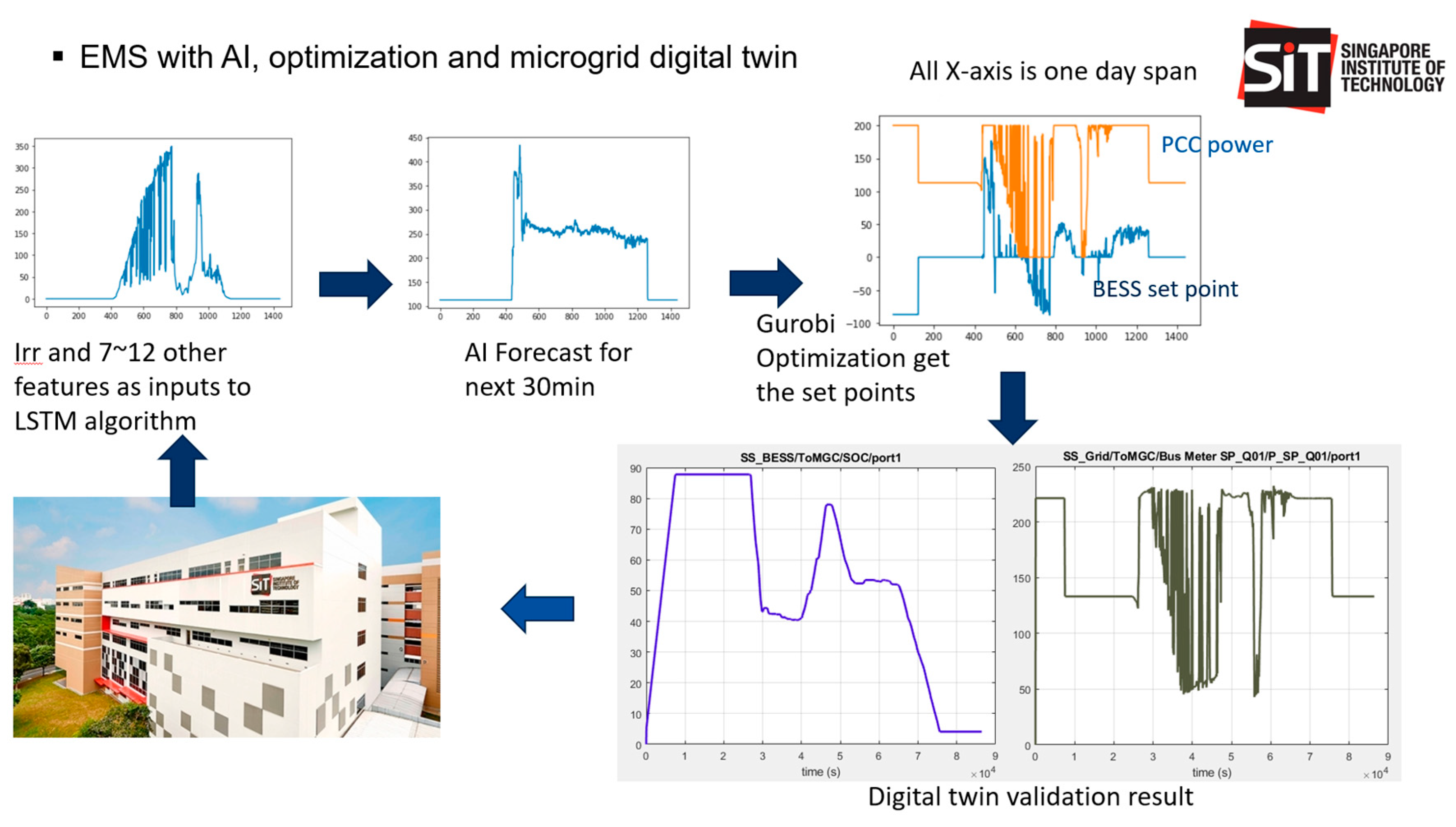
The research commences with an examination of the cooling system within the Smart Integrated Technologies (SIT) infrastructure at Nanyang Polytechnic (NYP). Subsequently, Long Short-Term Memory (LSTM) is employed to forecast the cooling load. These predictive outcomes are subsequently employed to formulate an efficient Battery Energy Storage System (BESS) operational plan aimed at optimizing building power consumption. To validate the efficacy of this operational strategy, a digital twin is utilized, thereby establishing a closed-loop feedback system for predictive power management, ultimately contributing to the enhancement of sustainable building operations. Below is a diagram (
Figure 1) illustrating the overall building predictive power control. With the real-time simulation in the digital twin, the proposed methodology can be running in both virtual or in real-time, parallel to the actual building management system.
In the ensuing sections, we provide a comprehensive exposition of the experimental specifics pertaining to each constituent element of the predictive building power control system.
2.1. Cooling system in SIT @ NYP
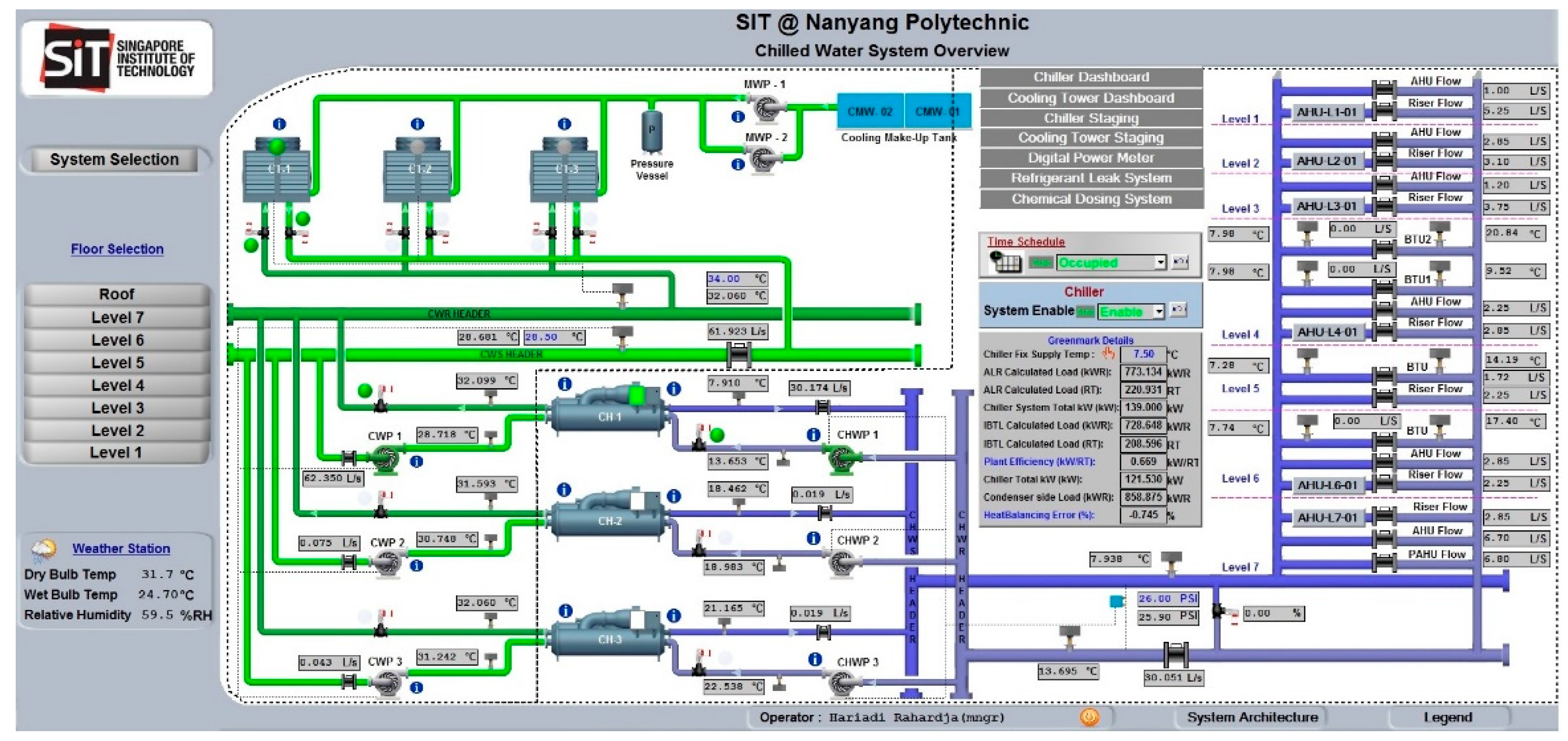
Overview of cooling system in SIT @ NYP building is shown in
Figure 2. Main components of cooling system are three units of cooling towers (CT), three units of chillers (CH), three units of chiller water pumps (CWP), three units of condenser water pumps (CHWP), Air Handling Units (AHU), and Fan Control Units (FCU). The system works together to regulate the temperature and flow of chilled water. The chilled water is supplied to AHU and FCU to condition air before it is distributed to the building space. Then, chilled water is returned to chiller to complete the chilled water circulation. In chiller (more specific in evaporator), returning chilled water will dump its heat the refrigerant to lower its temperature before it is supplied to AHU and FCU. The refrigerant will be released its heat at condenser water before it is circulated back to evaporator. The condenser water will be pumped to the cooling tower to reject the heat at the outdoor. Then, condenser water will be returned to chiller and ready to absorb some heat from the refrigerant. The AHU and FCU take fresh air from outside building then filter, dehumidify, and cool the air to the temperature specified by the BMS before it is distributed into the occupied spaces.
The building’s cooling system is automatically monitored and controlled by Honeywell Building Management System. It is designed to run only one unit at a time during normal periods but can run multiple units during periods of high demand.
2.2. Brief description of LSTM
Recurrent Neural Networks (RNNs) are ideal for time series prediction problems, where the input and output data are in sequential form. This is because RNNs have a feedback mechanism that allows them to consider previous input data to predict future values. However, one of the challenges of RNNs is the exploding and vanishing gradients that occur during the backpropagation step [
4]. This occurs because RNNs have a limited memory and as they go back in time during the backpropagation, the gradients become increasingly small, leading to vanishing gradients. To overcome this problem, Long Short-Term Memory (LSTM) networks are a variant of Recurrent Neural Network (RNN) that have been shown to have more stable gradient [
4,
5]. Hence, LSTM networks can capture long-term dependencies in data more effectively.
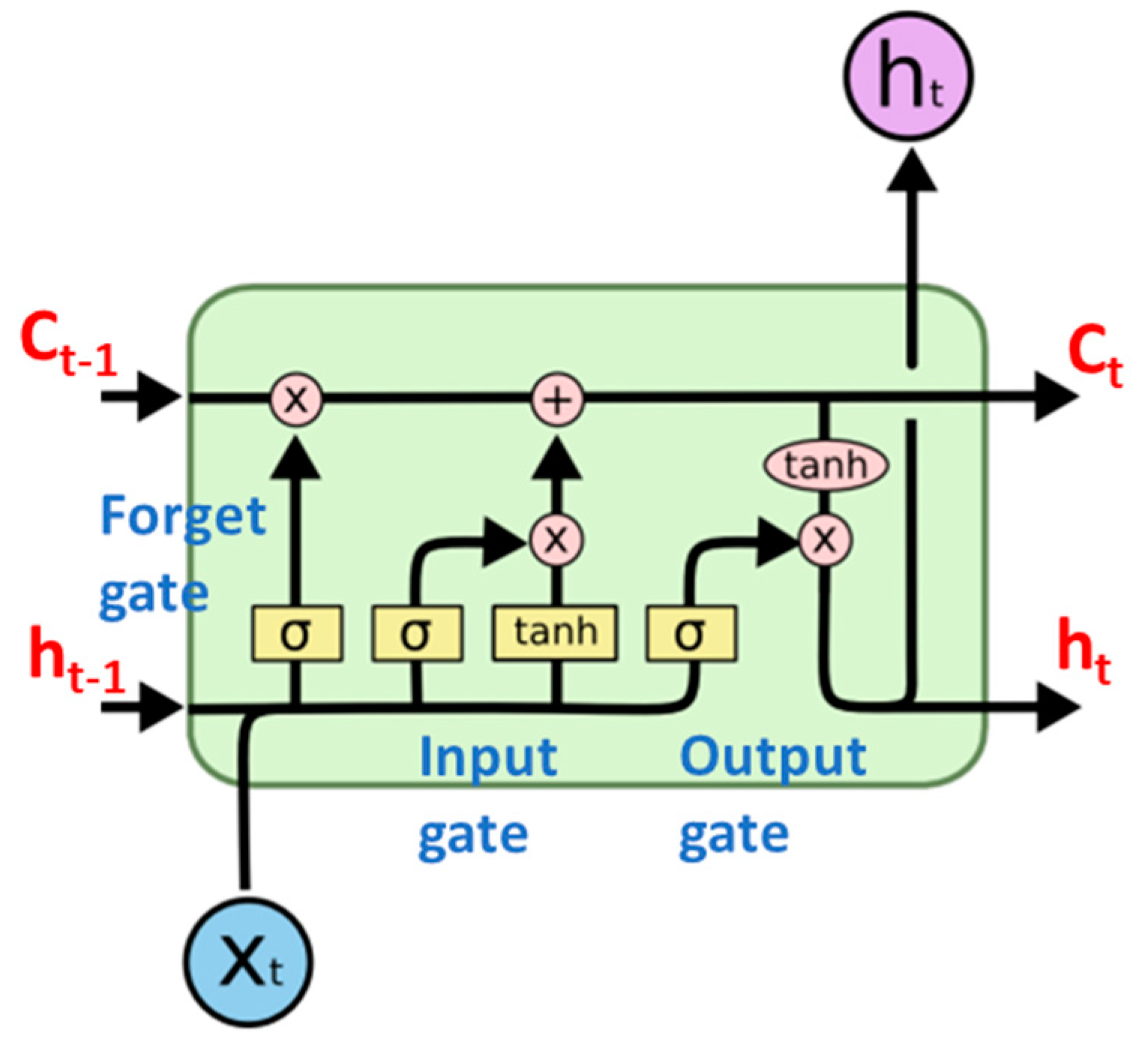
An LSTM networks consist of several key components, including the hidden state (
ht), cell state (
Ct), forget gate, input gate, and output gate as shown in
Figure 3. State is a memory unit of the networks that stores information, while gates regulate the flow of information into the state. Forget gate consists of sigmoid function, while both input and output gate consist of sigmoid and hyperbolic tangent function. Current input (X
t) and previous hidden state (h
t-1) is passed through the sigmoid function. If the output value of the sigmoid function is closer to 0 means forget and closer to 1 means to retain. The forget gate determines relevant information to keep from the prior cell state (C
t-1). The input gate decides relevant information to update in the current cell state (C
t) of the current LSTM unit. The output gate determines the present hidden state (h
t). Information from both cell state (C
t) and hidden state (h
t) will be passed to the next LSTM unit.
2.3. HVAC LSTM load predictor model
The LSTM networks [
6,
7] with one-layer and two-layers are examined and compared. The one-layer LSTM network has 100 hidden units, while the two-layer LSTM network has 100 hidden units in each layer. The features used in the study are pre-processed using standard scaling and min-max scaling techniques.
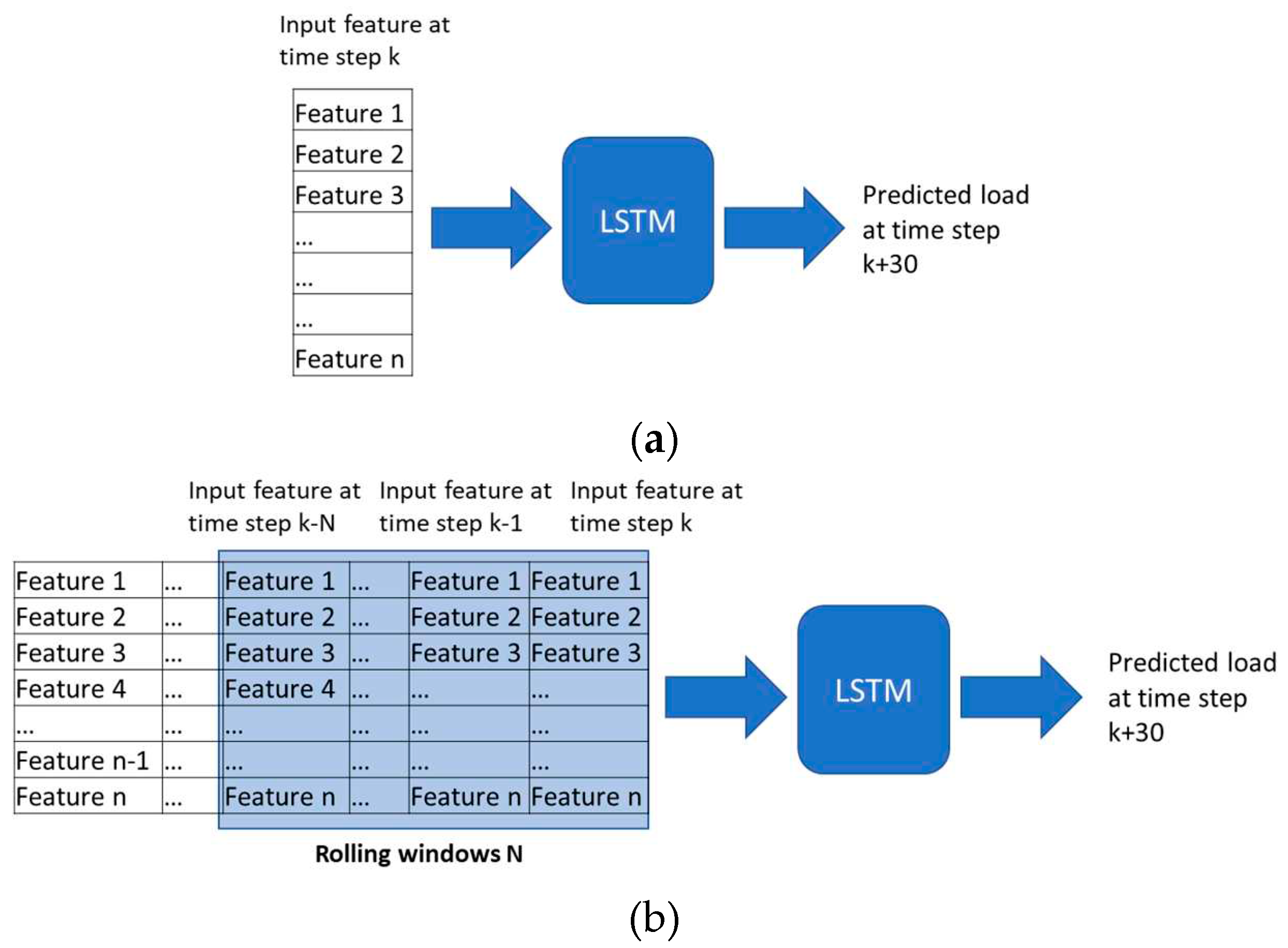
Two approaches are employed for estimating the HVAC load, known as LSTM-1 and LTSM-2. Both LSTMs are used to predict the load for the next 30 minutes and are based on the features listed in the
Table 1. Apart from different features used in each model, LSTM-1 is trained by using current features, meanwhile LSTM-2 is trained by using features in the rolling windows of past 20 minutes as shown in
Figure 4.
2.4. Energy management optimization using Gurobi
The microgrid concept is integral to modern energy systems, where energy storage emerges as essential components. This is particularly crucial given the dependency of Photovoltaic (PV) power generation on solar irradiance, a variable not subject to human control and contingent upon weather conditions. In the microgrid framework, a key player with high controllability assumes the responsibility of maintaining power and energy balance. This player adeptly adheres to setpoints established by the Microgrid Controller (MGC) or the estates operator. Frequently, BESS is the preferred and commonly employed technology for this purpose, exemplifying its significance in orchestrating the intricate dance of power generation and consumption within a microgrid setting. To ensure optimal functionality, BESS requires precise setpoints which will be dependent on the power control strategy.
To achieve optimal energy management, optimization is a must-to-do task. It needs to generate the setpoints for BESS. Gurobi is a highly utilized mathematical optimization solver and software bundle designed for addressing intricate linear and nonlinear programming challenges. [
10] Energy Supply and Demand Optimization using Gurobi is particularly valuable in the field of energy management, helping building owner make data-driven decisions to meet energy demand efficiently, reduce operational costs, and optimize resource utilization while considering various constraints and objectives.
As depicted in
Figure 1, the optimization process relies on several key input factors, including power generated by DER, building load demand forecasts generated by LSTM models, the prevailing electrical tariff, BESS and PV costs. The objective function of the optimization is determined by the building operator’s preferences and could encompass goals such as enhancing energy efficiency, lowering operational expenses, and optimizing resource utilization, among others.
In this section, the focus shifts to employing energy optimization techniques for the generation of Battery Energy Storage System (BESS) set-points, with consideration given to distinct scenarios.
Scenario 1, the primary objective is to attain the lowest cost of overall builder energy consumption. This involves a comprehensive evaluation that considers the electricity tariff from the main grid, as well as the costs associated with Photovoltaic (PV) power generation and BESS operation. The overarching aim is to curtail the total cost, thereby directly benefiting the builder user.
Scenario 2, the optimization process centers on minimizing infeed power fluctuation. High peak-to-peak demand fluctuations pose challenges for the main grid, necessitating additional resources and costs to accommodate sudden increases and decreases in power demand. By mitigating these fluctuations, the burden on the main grid is alleviated, especially in the context of an expanding microgrid landscape. Additionally, this approach contributes to the reduction of equipment sizes and associated costs, offering a dual advantage of enhanced grid stability and economic efficiency.
In Scenario 1: the objective function is to minimize the cost function below.
In Scenario 2: the objective function is to minimize the cost function below.
Where Pbat, Ppv, Pgrid are battery, PV, infeed grid power respectively. Cbat, Cpv, Cutility are cost of battery, PV and utility respectively. is the time step (1min in the scope of this study)
The constraints are:
- 1)
Battery SOC within limit at all time
- 2)
Battery SOC at the start of the day is the same as the end of day to ensure continuous operation of BESS.
- 3)
Maximum infeed power at PCC is 200kW at any time. And no power flow into the main grid.
- 4)
Power is balanced at all time
Pbat is the output variable which is then used as BESS setpoint in
Section 3.
2.5. Digital Twin modelling
Digital twinning of microgrid has become critical for effective projection of renewables and power source generation to meet the need of load demand. [
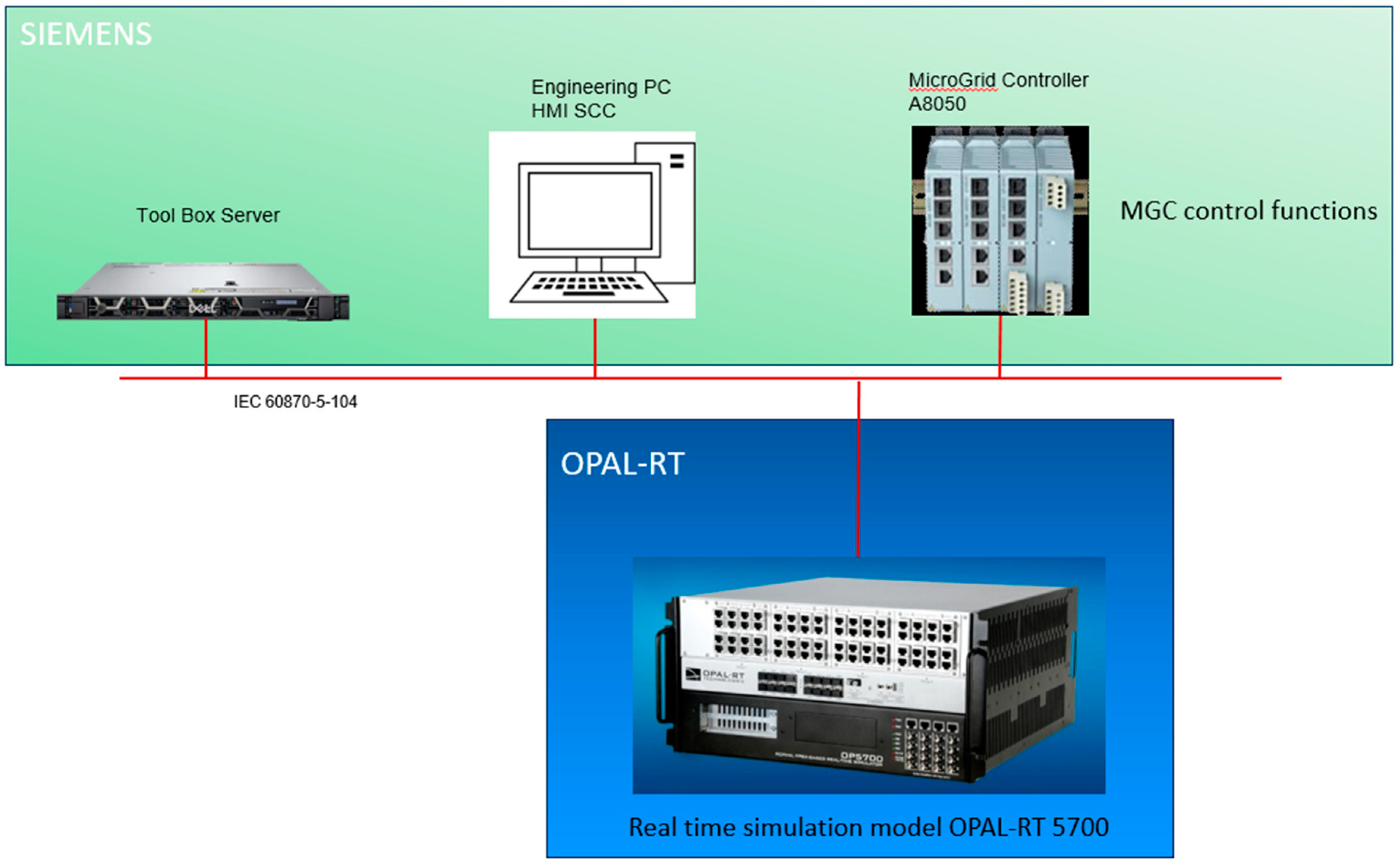
9] In this section, the potential application of microgrid in the building is studied. The microgrid is an experimental microgrid testbed set up in Singapore Power Concept Lab which is used to create a digital twin. The digital twin is created using the test data from the experimental microgrid and modeled in detail. It is based on hardware-controller-in-the-loop real-time simulation. The digital twin system architecture is shown in the
Figure 5. It consists of
- 1)
Siemens MGC
- 2)
Engineering PC
- 3)
Real-time simulator
- 4)
Toolbox Server
The digital twin is wired up using IEC 60870-104 communication protocol. MGC is the same model as in the experimental setup. MGC logic is replicated to the best effort to provide maximum accuracy in digital twin. The simulation model is built in details and running in real-time, enabling the digital twin to be able to model transient dynamic events and compatibility to connecting various hardware in the loop.
As the experimental microgrid and NYP building are of different energy scale, the following rating/capacities are altered to make a better match. The voltage and the rated power/ capacity are as shown in below
Table 1B.
Microgrid parameters.
Table 1B.
Microgrid parameters.
| Unit |
Voltage |
Rated Power/Capacity |
| PV |
415 V |
300kW |
| BESS |
275V/415 V |
300kW/200kWh |
| 2 x 1:1 transformer |
415V/415V |
400kVA |
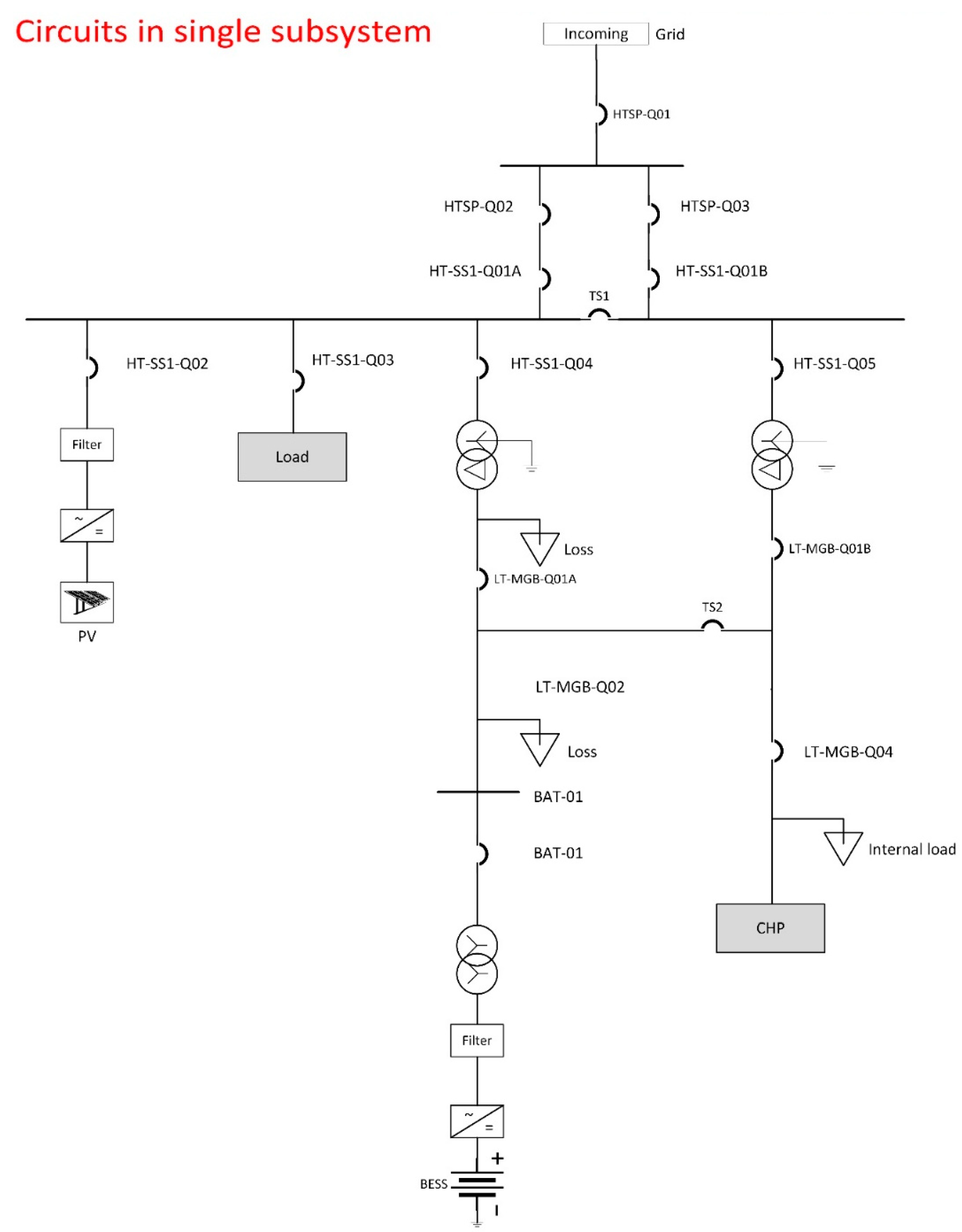
The circuit is shown in the figure below. The experimental microgrid is formed by a common busbar (HT-SS1). The PV is connected through PV inverter. The NYP load is represented by an aggregated load model. BESS is connected through a step-up transformer and a 1:1 transformer. The later one is for the safety reason and acting as an isolation barrier in case of faults on either building side or BESS side. Same principle applies for a backup combined heat and power generator (CHP). However, CHP is a back-up for islanded scenarios when there is a power outage on the main grid. CHP is more for energy reliability in contingencies and is not an economic DER in energy optimization. Hence, it is excluded in this paper.
The comprehensive validation and verification of the digital twin are elaborated upon [
11,
12], albeit regrettably omitted herein due to constraints imposed by page limitations. The outcomes attained in this study underscore a notable level of fidelity and accuracy. The research leverages the microgrid digital twin as a pioneering tool to substantiate the predictions expounded in
Section 3.1 and fine-tune the optimization procedures outlined in
Section 3.2. This methodological advancement is poised to significantly enhance the precision of predictive power control mechanisms within the context of sustainable buildings.
3. Results and Discussion
3.1. Cooling prediction
Different lengths and periods of training data, different architectures and scaling methods of LSTM are studied and discussed in this section.
3.1.1. LSTM-1
In first case, the LSTM-1 is trained by using Jul-Sep 2020 data.
Table 2 shows forecast accuracy of trained LSTM on different test data (Oct 2020, Sep 2022, and Oct 2022), architecture (one-layer and two-layers), and scaler (minmax and standard). Performance metrices used in the forecast are RMSE, MAE, and bias. For comparison over different models (one-layer LSTM MinMax scaler, one-layer LSTM Standard scaler, two-layers LSTM MinMax scaler, and two-layers LSTM Standard scaler) performance, average forecast performance of Oct 2020, Sep 2022, and Oct 2022 test data is also presented in
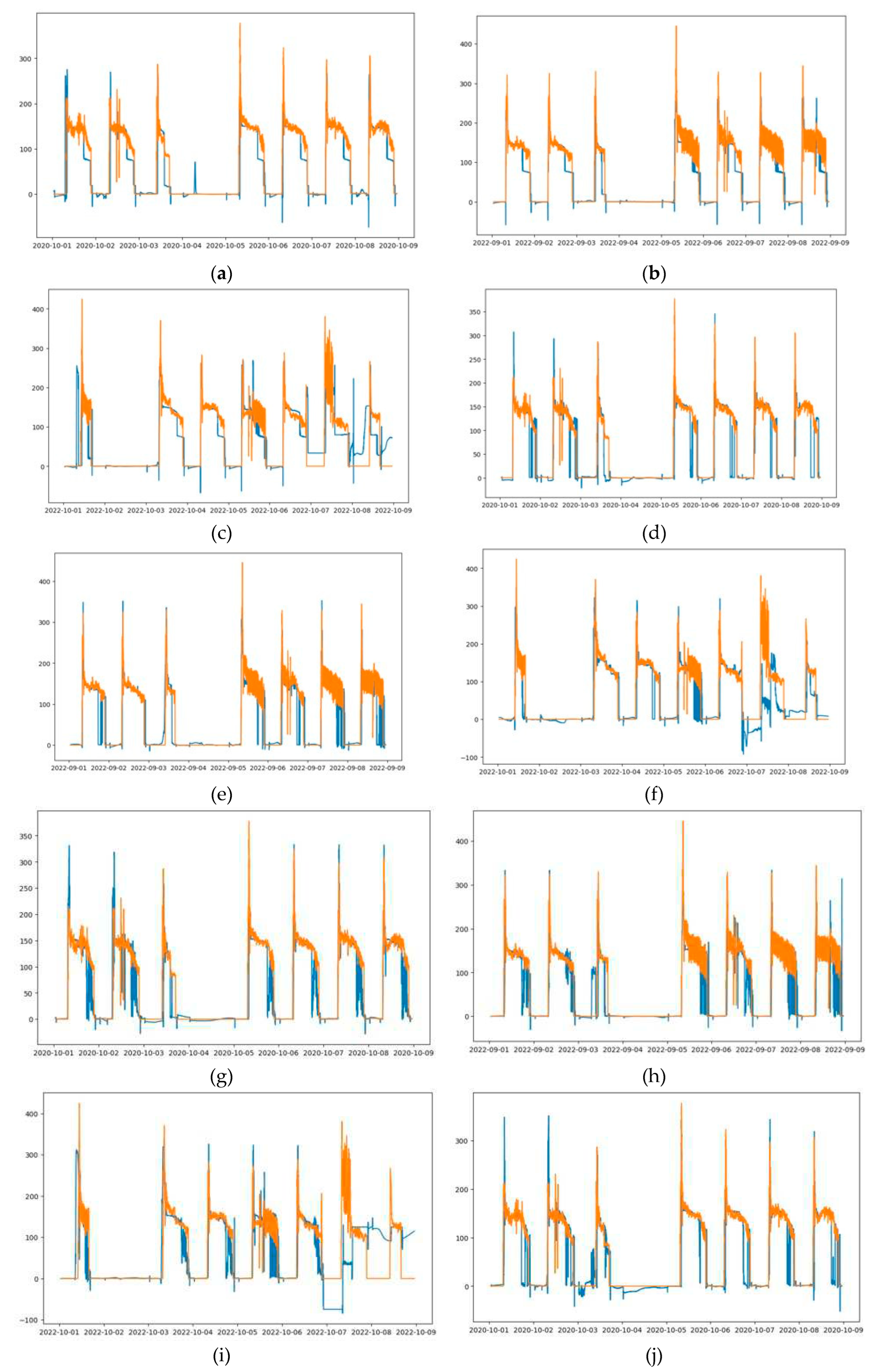
Table 2. The average results show that scaling method has quite significant influence on performance of the forecast accuracies. The one-layer LSTM Standard scaler has RMSE 23.8 kW, MAE 11.9 kW, and bias -2.5 kW, while the one-layer LSTM MinMax scaler has RMSE 33.9 kW, MAE 17 kW, and bias 11.5 kW. The two-layers LSTM Standard scaler has RMSE 22.5 kW, MAE 11.1 kW, and bias 0.4 kW, while the two-layers LSTM MinMax scaler has RMSE 28.1 kW, MAE 13.9 kW, and bias 1.6 kW. In both one-layer and two-layers LSTM architecture, the Standard scaler has outperformed MinMax scaler in term of performance metrices. The performance metrices RMSE and MAE of both one-layer and two-layers LSTM in Standard scaler are very similar. Thus, One-layer LSTM-1 Standard scaler works well to forecast the load. The forecast output of HVAC load in time series are presented in
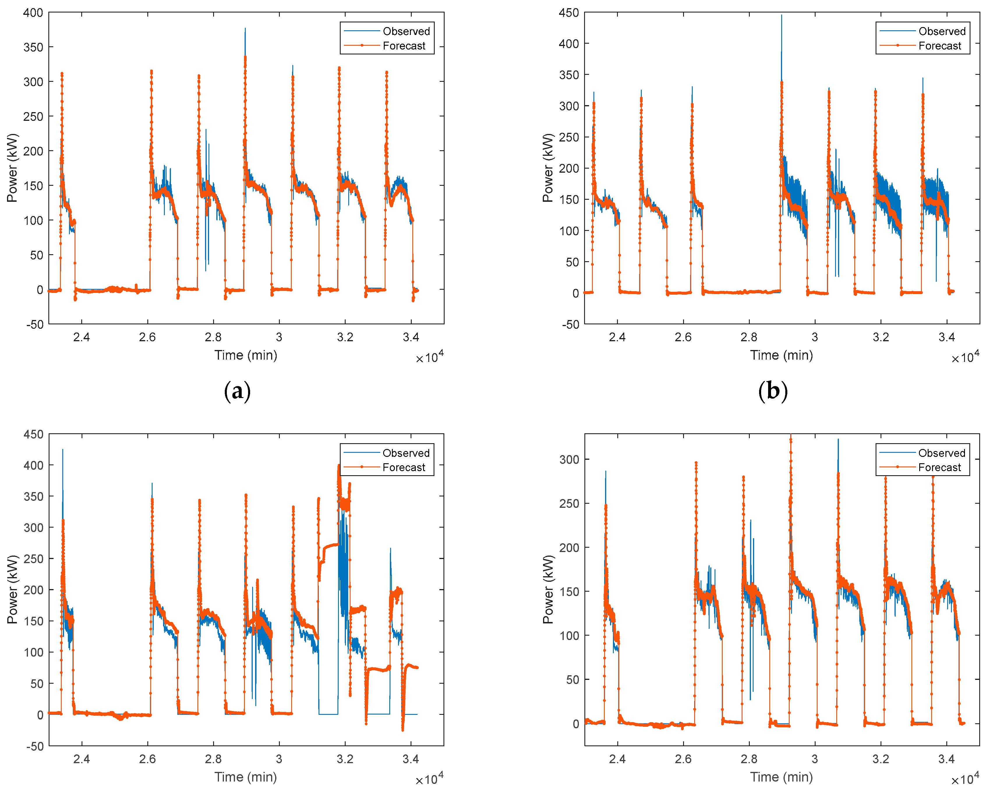
Figure 7.
In second case, LSTM-1 is trained by using short length of data from 1
st Sep 2022 to 6
th Sep 2022 while it makes forecast for next two days (7
th and 8
th Sep 2022). The forecast performance is presented in
Table 3. One-layer LSTM Standard scaler has RMSE 20.9 kW, MAE 11.9 kW, and bias 0.1 kW, while one-layer LSTM MinMax scaler has RMSE 21.4 kW, MAE 13.8 kW, and bias 5 kW. Two-layers LSTM Standard scaler has RMSE 22.6 kW, MAE 14.2 kW, and bias 2.1 kW, while the two-layers LSTM MinMax scaler has RMSE 26 kW, MAE 17.8 kW, and bias 11.1 kW. The best model is one-layer LSTM Standard scaler.
In both cases, one-layer LSTM with Standard scaler outperform other models and accuracies of the prediction are not necessary to improve due to increase number of layers in LSTM.
3.1.2. LSTM-2
Similar with LSTM-1, the LSTM-2 is trained by using Jul-Sep 2020 data in the first case.
Table 3 shows forecast accuracy of trained LSTM on different test data, architecture, and scaler. Average forecast performance of Oct 2020, Sep 2022, and Oct 2022 test data is presented in
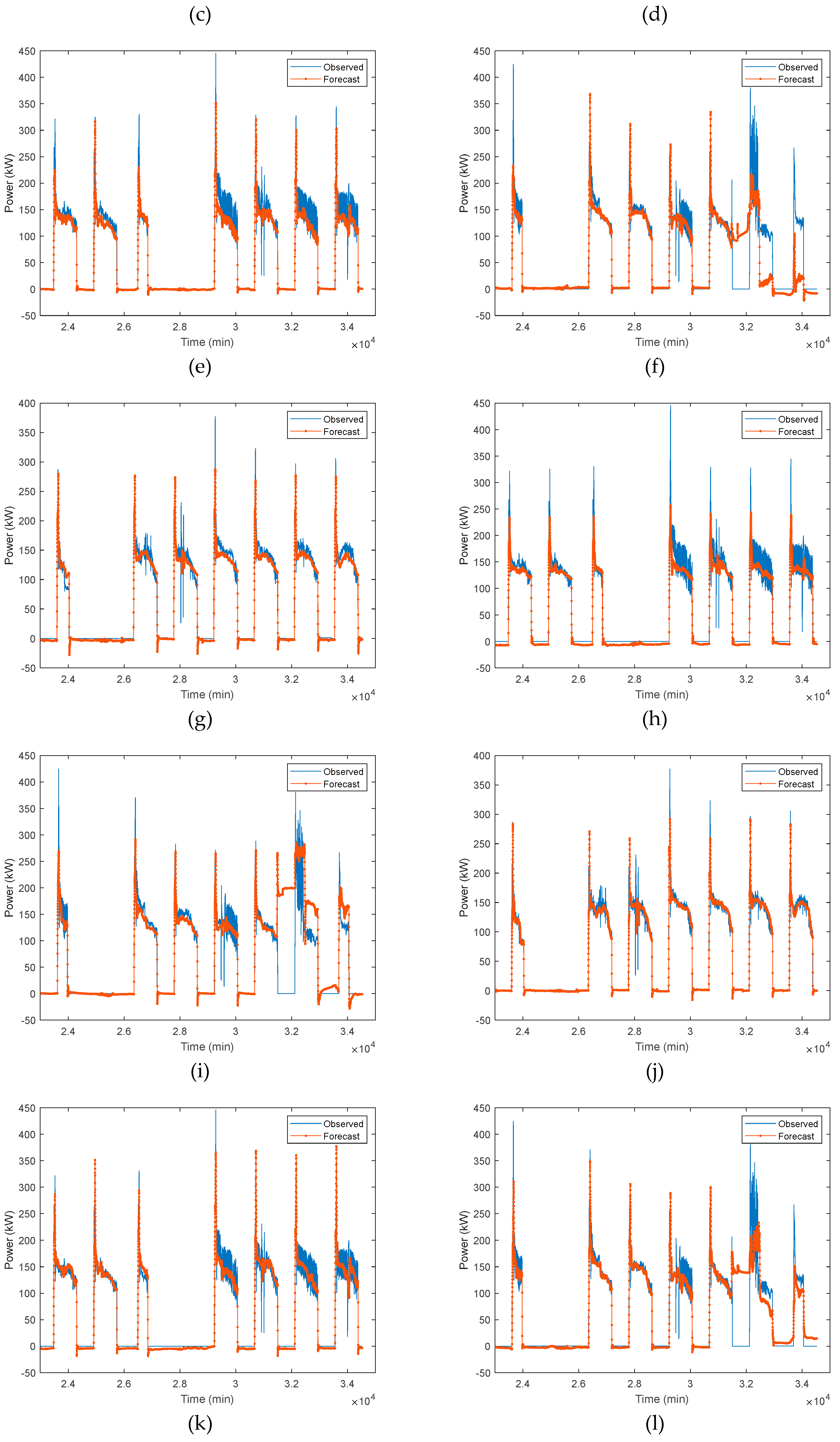
Table 4. One-layer LSTM Standard scaler has RMSE 45.27 kW, MAE 20 kW, and bias 8.58 kW, while the one-layer LSTM MinMax scaler has RMSE 37.03 kW, MAE 18.43 kW, and bias 4 kW. The two-layers LSTM Standard scaler has RMSE 46.17 kW, MAE 20.97 kW, and bias 7.02 kW, while the two-layers LSTM MinMax scaler has RMSE 49.07 kW, MAE 23.8 kW, and bias 6.3 kW. From these results, one-layer LSTM MinMax scaler has the least RMSE, MAE, and bias error among other models. The forecast output of HVAC load in time series are presented in
Figure 8.
Similar with LSTM-1, the LSTM-2 in second case is trained by using data from 1
st Sep 2022 to 6
th Sep 2022 data while the forecasting period is from 7
th Sep 2022 to 8
th Sep 2022. The forecast performance is presented in
Table 5. One-layer LSTM Standard scaler has RMSE 22.41 kW, MAE 13.07 kW, and bias -3.12 kW, while one-layer LSTM with MinMax scaler has RMSE 21.22 kW, MAE 12.28 kW, and bias -1.52 kW. Two-layers LSTM with Standard scaler has RMSE 23.7 kW, MAE 13.18 kW, and bias -1.57 kW, while the two-layers LSTM with MinMax scaler has RMSE 23.73 kW, MAE 13.18 kW, and bias -2.21 kW. The best model is one-layer LSTM MinMax scaler which similar with first case.
Based on both LSTM-1 and LSTM-2 results, one-layer LSTM work sufficiently accurate to predict HVAC cooling load. For the choice of scaling, it is dependent on the type of model used in the prediction.
3.2. Energy optimization in microgrid.
As concluded in
Section 3.1, one layer LSTM is sufficiently accurate to predict the cooling load. The cooling load in NYP can be accurately predicted. In this section, one day (1
st Sep 2022, trained using Jul 2020 and Sep 2020 data, one-layer LSTM) is taken as an example sample to conduct the energy optimization. Besides the cooling load, there are static load in the building which is running 24/7, such as server room. Adding the static load and cooling load, the total load demand in the building can be obtained. Below is the actual vs predicted total load in the building.
The electric tariff is set to 0.2996 SGD/kWh with reference to Singapore’s utility price in 3rd quarter 2023. The electrical tariff is assumed to provide incentive to consumers to use power during off-peak period. The off-peak price is set to 0.18 SGD/kWh. The cost of battery is set to 0.1715 SGD/kWh usage with reference to the cost projection for battery storage provided by National Renewable Energy Laboratory. The cost of PV is neglected as the PV system can last for 20~30 years with low maintenance cost.
Scenario 1 is further separated into Scenario 1A- lowest cost with fixed SOC0 and Scenario 1B-lowest cost. SOC0 is the initial battery SOC. In Scenario 1A, SOC0 is fixed at 50%. In Scenario 1B, SOC0 is flexible and become one of the variables to solve. In all scenarios, battery SOC limit is set to 5~95%.
Scenario 1A: lowest cost with Fixed SOC0 (LCFS).
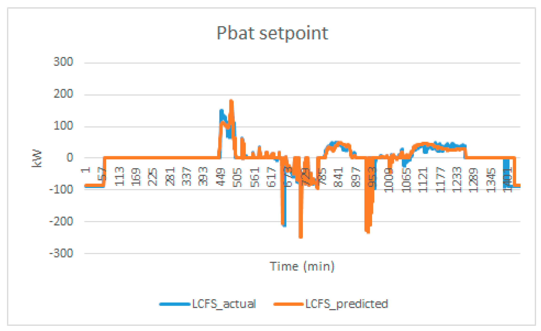
The actual optimal energy management profile (BESS power setpoint) and predicted optimal energy management profile is in shown
Figure 10.
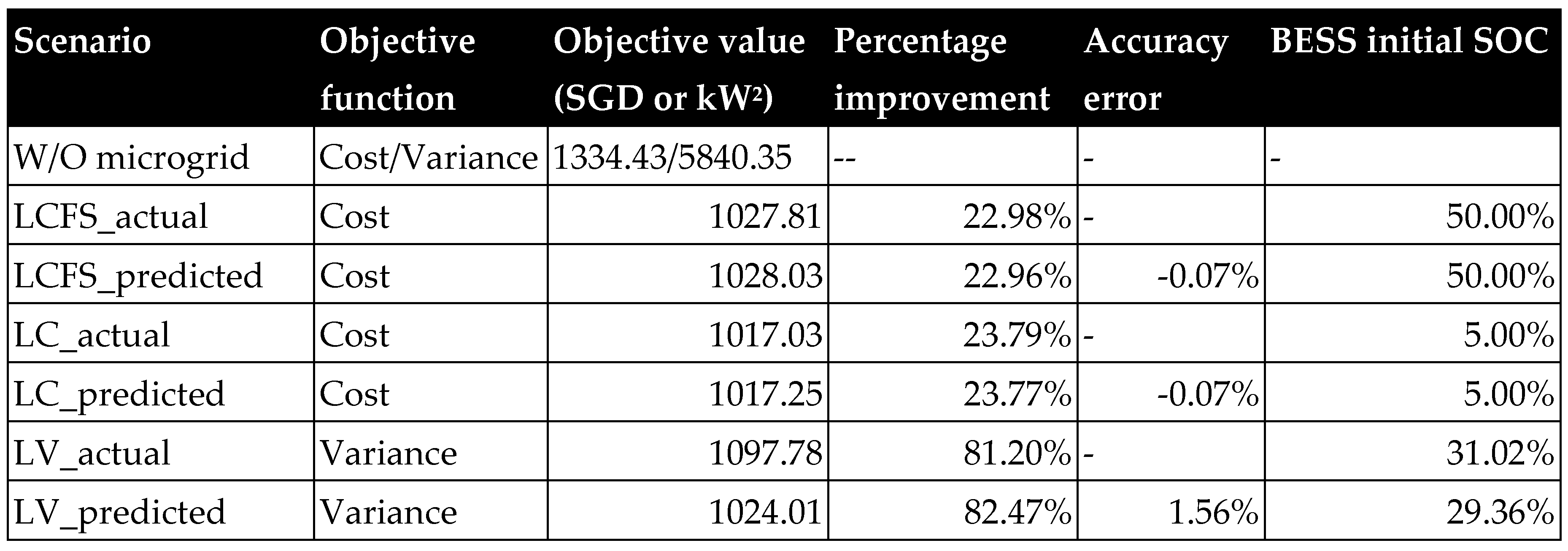
The result reveals that the predicted optimal provide an accurate BESS power setpoint. The resulting LCFS predicted electricity cost is 1028.03 SGD as compared to the actual 1027.81 SGD. Without the microgrid, the electricity cost is 1334.43 SGD. The reduction in energy cost is 306.4 SGD.
Scenario 1B: lowest cost (LC).
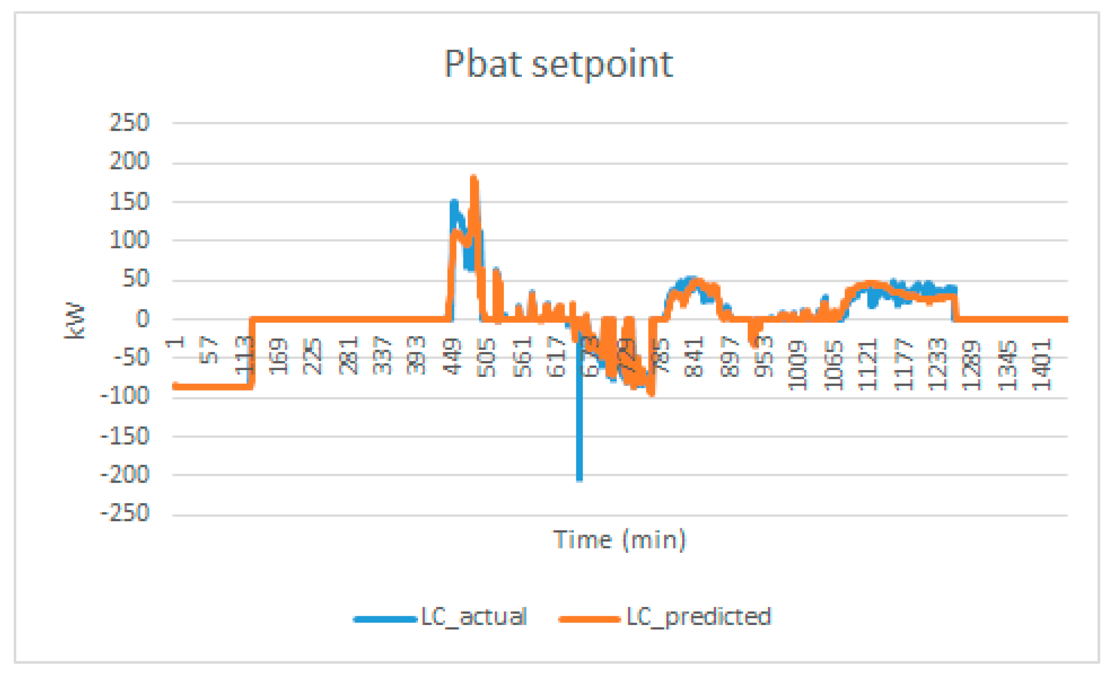
The actual optimal energy management profile (BESS power setpoint) and predicted optimal energy management profile is shown in
Figure 11.
The graphical representation illustrates that the predicted optimal solution effectively aligns with the true BESS power set-point. As a consequence, the forecasted LCFS electricity cost amounts to 1017.25 SGD, closely approximating the actual cost of 1017.03 SGD. In the absence of the microgrid infrastructure, the electricity cost rises to 1334.43 SGD. This discernible disparity results in a noteworthy reduction in energy-related expenditures, amounting to 317.18 SGD. In this case, the flexible SOC0 provides extra energy reduction. The optimal SOC0 at the beginning of the day is 5%, the lower limit of SOC defined.
Scenario 2: lowest Variance (LV).
The variance of grid power serves as a pivotal metric denoting the oscillation in power load. As exemplified by the observed electrical load requisites, the zenith of power demand culminates at 428.85 kW. In the context of high-tension power supplies, the rate applied to contracted capacity is more favorable in comparison to uncontracted capacity, signifying an economic incentive for responsible capacity planning. It is imperative to acknowledge that an elevated variance in power consumption substantially heightens the likelihood of incurring expenses related to uncontracted capacity, accentuating the financial significance of minimizing load fluctuations and optimizing capacity utilization.
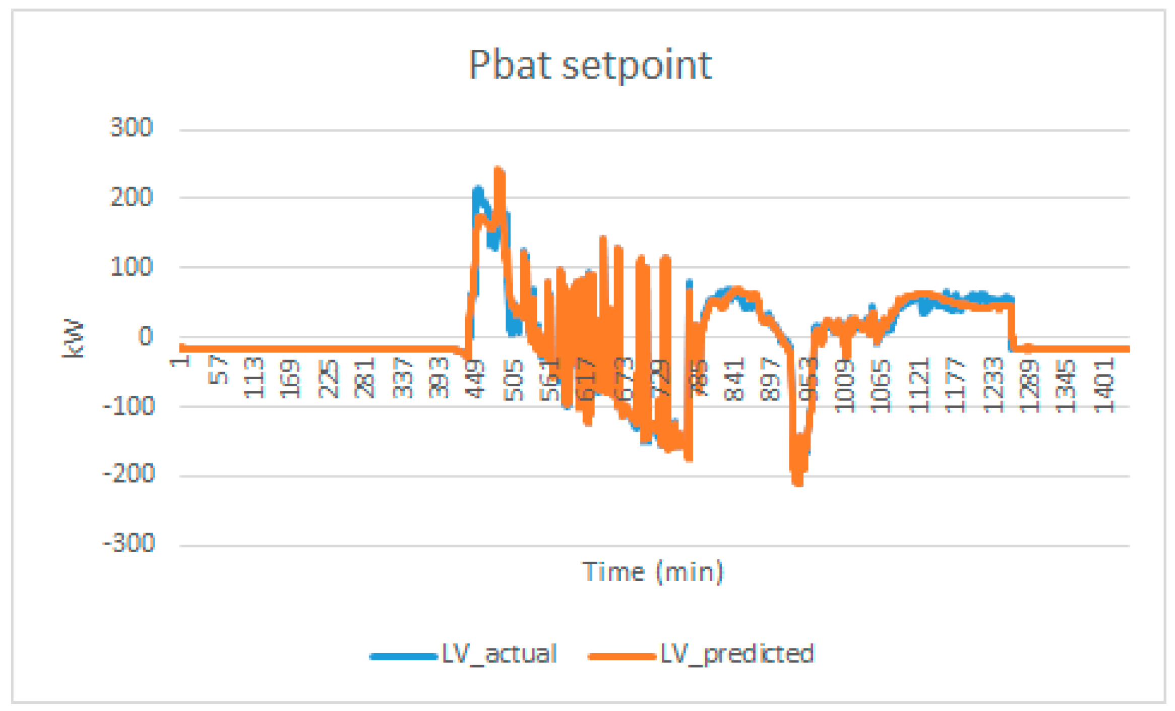
The result of LV optimization for actual load demand and predicted load demand is shown in
Figure 13. The LV optimization using predicted load data is 1024.01
which is lower than the 1097.78
. This is due to more fluctuation in the actual load demand than the prediction. The results of the optimization process are summarized in the
Table 6.
3.3. Microgrid digital twin result and discussion
Following
Section 3.2, the optimized setpoints are used as the reference in the microgrid digital twin system. The result achieved reveals a close-to-reality performance of microgrid integration with SIT@NYP campus. The objective is to verify the results from
Section 3.1 and 3.2. The findings from microgrid digital twin reveal the discrepancies due to physical microgrid and gives feedback to the building predictive power control.
Scenario 1A: lowest cost with Fixed SOC0 (LCFS).
In this scenario, the actual power demand that is required from the grid is plotted as in
Figure 13.
The actual power needed from grid is based on the optimization of the actual building load, which is the optimal energy management in an ideal scenario. The predicted power needed from grid is based on the optimization of the predicted building load demand using LSTM. The result shows a close match between two scenarios. the battery is charging during mid-night period. During charging, the battery charging solution is not unique, the time of charging is flexible given that it will not affect the value of objective function. Hence, the grid power consumption at the end of the day is different between actual and predicted load.
In both actual and predicted cases, the optimization process gives a lower power consumption from the main grid. In physical microgrids, energy conversion efficiency always introduces power loss in the system. Besides, there are various ancillary devices required for microgrids operation such as, industrial PC, controller, data servers etc. Hence, the microgrid digital twin reveals the power consumption that is closer to the real-world application.
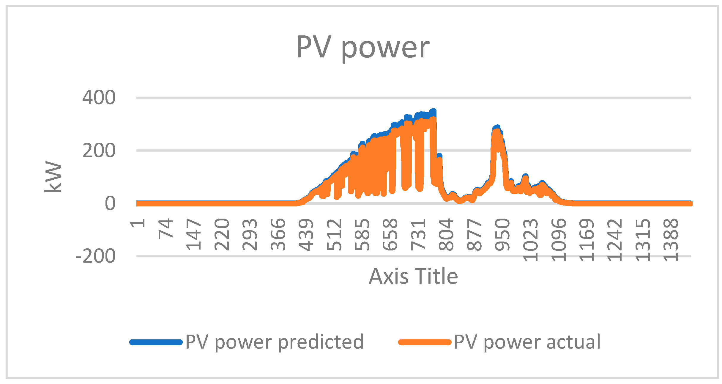
Figure 14 shows solar energy conversion efficiency. The actual power generated is lower as compared to the predicted PV power.
Scenario 1B: lowest cost (LC).
In this scenario, the actual power demand that is required from the grid is plotted as in
Figure 15.
In this scenario, initial battery SOC is flexible. After digital twin simulation, it was observed that grid power demand has a similar trend as in Scenario 1A. There is an additional power required from grid. The battery is at 5% SOC in the beginning of the day and is charged early in the morning to take advantage of the lower electricity price in off-peak hour.
Scenario 2: lowest Variance (LV).
In this scenario, the focus is to reduce the power fluctuations so that the power variance is minimized. The result from digital twin is plotted in Figure 17. The power fluctuation from the DT is much higher as compared with the ideal optimization. However, due to the additional power consumption in microgrid, the variance is decreased in DT.
Figure 15.
Grid power demand comparison in Scenario 2.
Figure 15.
Grid power demand comparison in Scenario 2.
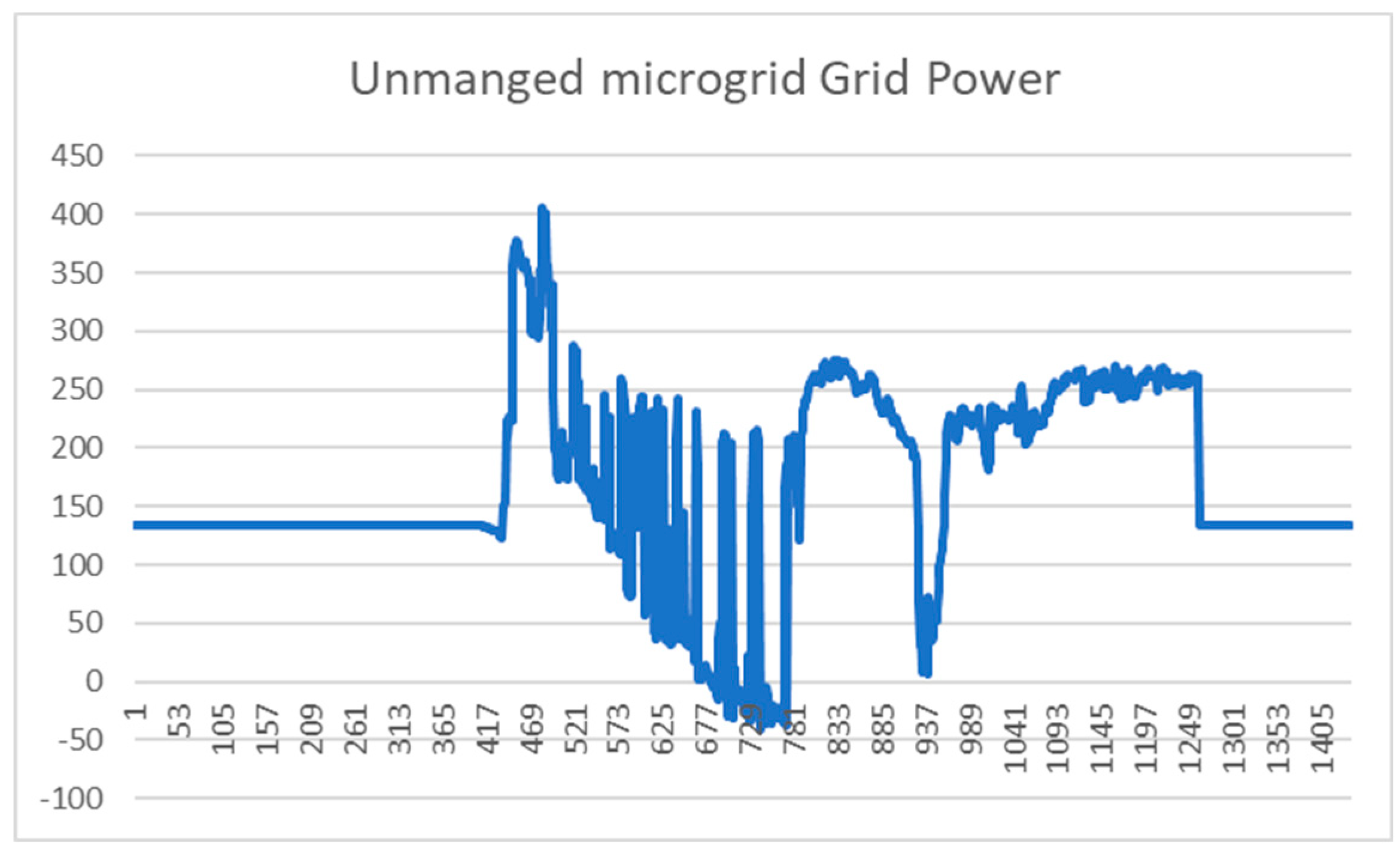
When the microgrid is unmanaged, namely, BESS is not active, the power drawn from grid is shown in the figure below:
Figure 16.
Grid power demand in unmanaged microgrid scenario.
Figure 16.
Grid power demand in unmanaged microgrid scenario.
As compared to the unmanaged case, the peak power demand is reduced from 405.47kW to (229.79kW, 232.94kW) in digital twin verified result. This significant reduction in the peak power will benefit both the builder owner as well as the grid provider. The size of the equipment (Such as transformer, protection device) can be reduced for SIT@NYP building and the user can subscribe to smaller contracted capacity. Hence, it will bring economic benefits to the stakeholders.
4. Conclusion
In summary the authors present a systematic way of combining AI, Optimization and microgrid digital twin to form a novel way to predictive power control to building. The results show promising accuracy and accountability. In the prediction analysis, the result reveals that for buildings with cyclic power demand, the load is highly predictable and one layer LSTM can provide sufficiently good prediction regardless of training data date (pre covid or during covid). The optimization process shows performance improvement from 22% to 82% depending on the builder operator’s preference. The microgrid digital twin shows the dilemma in actual microgrid. There is un-negligible energy lost due energy conversion efficiency as well as ancillary devices. The feedback from microgrid digital twin system can then be used as feedback in the optimization process to improve the accuracy.
In future, or when physical microgrid is implemented, the real-time digital twin can provide online energy prediction and optimization which can operate in parallel with the building electrical and cooling system. It will further unleash the power of microgrid digital twin in predictive power control to building sustainability.
Funding
This project is supported by the National Research Foundation, Singapore, and the Energy Market Authority, under the Exploiting Distributed Generation (“EDGE”) Programme and administered by the EDGE Programme Office (EDGE Programme Award EDGE-GC2018-001). Any opinions, findings and conclusions or recommendations expressed in this material are those of the author(s) and do not reflect the views of Energy Market Authority, Singapore.
References
- F.Mtibaa , K.-K. Nguyen, M.Azam, A. Papachristou et al, “LSTM-based indoor air temperature prediction framework for HVAC systems in smart buildings”. Neural Computing and Applications 32(3). [CrossRef]
- S. F.Ahmed, Md. S. B.Alam, M. Hassan, M. R. Rozbu, T. Ishtiak, N. Rafa, M. Mofijur, A. B. M. Shawkat Ali & Amir H. Gandomi, “Deep learning modelling techniques: current progress, applications, advantages, and challenges”, Artificial Int. Rev. 56, pp13521 – 13617 (2023). [CrossRef]
- H. S. Lim, G. Kim, “Prediction model of Cooling Load considering time-lag for preemptive action in buildings” Energy Build. 151, 53–65 (2017). [CrossRef]
- J. Zhang, Y. Zeng, B. Starly, “Recurrent neural networks with long term temporal dependencies in machine tool wear diagnosis and prognosis” SN Applied Science, 3, 442 (2021). [CrossRef]
- Q. Wang, R-Q. Peng, J.-Q. Wang, Z. Li, H-B. Qu, “NEWLSTM: An Optimized Long Short-Term Memory Language Model for Sequence Prediction”, IEEE , pp65395-65401 (2020). [CrossRef]
- C. Zhou, Z. Fang, X. Xu, X. Zhong. Y. Ding. X. Jiang, Y. Ji “Using long short-term memory networks to predict energy consumption of air-conditioning systems”, Sustainable Cities and Society, v55, p10200 (2020). [CrossRef]
- M Mavsar, M Deniša, B Nemec, A Ude, “Intention Recognition with Recurrent Neural Networks for Dynamic Human-Robot Collaboration”, IEEE Conf.: 2021 20th International Conference on Advanced Robotics (ICAR). [CrossRef]
- R. Chalapathy, N. L. D. Khoa, S. Sethuvenkatraman “Comparing multi-step ahead building cooling load prediction using shallow machine learning and deep learning models” Sust. Energy, Grids and Networks, 28 p100543 (2021). [CrossRef]
- Y. Cui, F. Xiao. W. Wang, X. He, C. Zhang, Y. Zhang et al, “Digital Twin for Power System Steady-state Modelling, Simulation, and Analysis”, 2020 IEEE 4th Conference on Energy Internet and Energy System Integration (EI2). [CrossRef]
- T. Iqbal, Z. Khitab, F. Girbau, A. Sumper at el, “Energy Management System for Optimal Operatioin of Microgrids Network” 2018 IEEE International Conference on Smart Energy Grid Engineering (SEGE). [CrossRef]
- H. Jiang, Rudy Tjandra, W. J. Lim, S. Cao, C. B. Soh, K. T.Tan, Sivaneasan B.Krishnan, "Unleashing the Potential of Digital Twin Technology in Microgrid – A Case Study of a Tropical Microgrid", 2023 6th International Conference on Electrical Engineering and Green Energy (CEEGE), pp.165-170, 2023. [CrossRef]
- Wei Feng, Chen Xuebing, Cao Shuyu, Soh Chew Beng, Cai Zhiqiang, Tseng King Jet, D. Mahinda Vilathgamuwa, "MPC Based Dynamic Voltage Regulation Using Grid-Side BESPS With the Consideration of Communication Delay", IEEE Transactions on Energy Conversion, vol.38, no.2, pp.838-848, 2023. [CrossRef]
- W. WANG. J. Wang, J. Tian, J. Lu, R. Xiong, “Application of Digital Twin in Smart Battery Management Systems”, Chin. J. Mech. Eng. 2021) 34:57. [CrossRef]
Figure 1.
Overview of predictive building power control using AI, energy optimization and microgrid digital twin platform.
Figure 1.
Overview of predictive building power control using AI, energy optimization and microgrid digital twin platform.
Figure 2.
Overview of SIT @ Nanyang Polytechnic chilled water system.
Figure 2.
Overview of SIT @ Nanyang Polytechnic chilled water system.
Figure 3.
Diagram of LSTM [
6].
Figure 3.
Diagram of LSTM [
6].
Figure 4.
Time series inputs configuration to LSTM. The network in (a) LSTM-1 requires current input feature and (b) LSTM-2 requires rolling windows N.
Figure 4.
Time series inputs configuration to LSTM. The network in (a) LSTM-1 requires current input feature and (b) LSTM-2 requires rolling windows N.
Figure 5.
Digital Twin architecture which comprises of Siemens MGC, Engineering PC, Real-time simulator and Toolbox server.
Figure 5.
Digital Twin architecture which comprises of Siemens MGC, Engineering PC, Real-time simulator and Toolbox server.
Figure 6.
Circuit in Single Sub-system.
Figure 6.
Circuit in Single Sub-system.
Figure 7.
Measured load vs. predicted load (a)-(c) One-layer LSTM-1 MinMax scaler; (d)-(f) One-layer LSTM-1 Standard scaler, (g)-(i) Two-layers LSTM-1 MinMax scaler, and (j)-(l) Two-layers LSTM-1 Standard scaler. (a), (d), (g), and (j) 1st week of Oct 2020 test data. (b), (e), (h), and (k) 1st week of Sep 2022 test data. (c), (f), (i), and (l) 1st week of Oct 2022 test data.
Figure 8.
Measured load vs. predicted load (a)-(c) One-layer LSTM-1 MinMax scaler; (d)-(f) One-layer LSTM-1 Standard scaler, (g)-(i) Two-layers LSTM-1 MinMax scaler, and (j)-(l) Two-layers LSTM-1 Standard scaler. (a), (d), (g), and (j) 1st week of Oct 2020 test data. (b), (e), (h), and (k) 1st week of Sep 2022 test data. (c), (f), (i), and (l) 1st week of Oct 2022 test data.
Figure 9.
Left: Actual load demand vs predicted load demand. Right: Irradiance for the day.
Figure 9.
Left: Actual load demand vs predicted load demand. Right: Irradiance for the day.
Figure 10.
BESS power setpoint in Scenario 1A, actual optimal vs predicted optimal.
Figure 10.
BESS power setpoint in Scenario 1A, actual optimal vs predicted optimal.
Figure 11.
BESS power setpoint in Scenario 1B, actual optimal vs predicted optimal.
Figure 11.
BESS power setpoint in Scenario 1B, actual optimal vs predicted optimal.
Figure 12.
BESS power setpoint in Scenario 2, actual optimal vs predicted optimal.
Figure 12.
BESS power setpoint in Scenario 2, actual optimal vs predicted optimal.
Figure 13.
Grid power demand in Scenario 1A, actual vs predicted in optimization and DT simulation.
Figure 13.
Grid power demand in Scenario 1A, actual vs predicted in optimization and DT simulation.
Figure 14.
Predicted PV power vs actual PV power.
Figure 14.
Predicted PV power vs actual PV power.
Figure 15.
Grid power demand in Scenario 1B, actual vs predicted in optimization and DT simulation.
Figure 15.
Grid power demand in Scenario 1B, actual vs predicted in optimization and DT simulation.
Figure 16.
Grid power demand in Scenario 2, actual vs predicted in optimization and DT simulation.
Figure 16.
Grid power demand in Scenario 2, actual vs predicted in optimization and DT simulation.
Table 1.
List of features used in both LSTM-1 and LSTM-2.
Table 1.
List of features used in both LSTM-1 and LSTM-2.
| No |
Feature |
LSTM-1 |
LSTM-2 |
Notes |
| 1 |
chiller water supply temperature |
Yes |
Yes |
|
| 2 |
chiller water return temperature |
Yes |
Yes |
|
| 3 |
chiller water flow |
Yes |
Yes |
|
| 4 |
compressor water supply temperature |
Yes |
Yes |
|
| 5 |
compressor water return temperature |
Yes |
Yes |
|
| 6 |
compressor water flow |
Yes |
Yes |
|
| 7 |
calculated load tonnage |
Yes |
No |
|
| 8 |
heat out |
Yes |
No |
|
| 9 |
total HVAC cooling load |
Yes |
No |
Total HVAC cooling load recorded by BMS |
| 10 |
wet bulb temperature |
Yes |
No |
Weather station measurement |
| 11 |
ambient temperature |
Yes |
No |
Weather station measurement |
| 12 |
Irradiation |
Yes |
No |
Weather station measurement |
| 13 |
HVAC on/off |
Yes |
No |
Scheduled HVAC system turn on/off |
| 14 |
Day of week |
No |
Yes |
Weekday: 0,
Saturday: 0.5,
andSunday: 1 |
| 15 |
Minute of day |
No |
Yes |
Minutes of the day |
Table 2.
Prediction results of LSTM-1 based on Jul-Sep 2020 trained data.
Table 2.
Prediction results of LSTM-1 based on Jul-Sep 2020 trained data.
| Architecture |
Scaling |
Train Data |
Test Data |
RMSE |
MAE |
Bias |
| One-layer LSTM |
MinMax |
Jul to Sep 2020 |
Oct 2020 |
11.81 |
5.67 |
-1.03 |
| MinMax |
Jul to Sep 2020 |
Sep 2022 |
15.23 |
7.36 |
0.68 |
| MinMax |
Jul to Sep 2020 |
Oct 2022 |
74.63 |
38.04 |
34.89 |
| |
|
|
Mean |
33.9 |
17 |
11.5 |
| One-layer LSTM |
Standard |
Jul to Sep 2020 |
Oct 2020 |
11.6 |
5.82 |
2.4 |
| Standard |
Jul to Sep 2020 |
Sep 2022 |
18.18 |
8.88 |
-5.2 |
| |
Standard |
Jul to Sep 2020 |
Oct 2022 |
41.86 |
21.2 |
-4.72 |
| |
|
|
Mean |
23.8 |
11.9 |
-2.5 |
| Two-layers LSTM |
MinMax |
Jul to Sep 2020 |
Oct 2020 |
12.75 |
7.71 |
-3.13 |
| MinMax |
Jul to Sep 2020 |
Sep 2022 |
19.1 |
11.11 |
-6.16 |
| MinMax |
Jul to Sep 2020 |
Oct 2022 |
52.44 |
23.05 |
14.17 |
| |
|
|
Mean |
28.1 |
13.9 |
1.6 |
| Two-layers LSTM |
Standard |
Jul to Sep 2020 |
Oct 2020 |
11.3 |
4.83 |
-0.87 |
| Standard |
Jul to Sep 2020 |
Sep 2022 |
16.94 |
9.92 |
-1.53 |
| |
Standard |
Jul to Sep 2020 |
Oct 2022 |
39.36 |
18.54 |
3.72 |
| |
|
|
Mean |
22.5 |
11.1 |
0.4 |
Table 3.
Prediction results of LSTM-1 based on 1st - 6th Sep 2022 trained data.
Table 3.
Prediction results of LSTM-1 based on 1st - 6th Sep 2022 trained data.
| Architecture |
Scaling |
Train Data |
Test Data |
RMSE |
MAE |
Bias |
| One-layer LSTM |
MinMax |
1st - 6th Sep 2022 |
7th - 8th Sep 2022 |
21.48 |
13.83 |
5.01 |
| One-layer LSTM |
Standard |
1st - 6th Sep 2022 |
7th - 8th Sep 2022 |
20.98 |
11.91 |
0.17 |
| Two-layers LSTM |
MinMax |
1st - 6th Sep 2022 |
7th - 8th Sep 2022 |
26.02 |
17.79 |
11.17 |
| Two-layers LSTM |
Standard |
1st - 6th Sep 2022 |
7th - 8th Sep 2022 |
22.64 |
14.25 |
2.08 |
Table 4.
Prediction results of LSTM-2 based on Jul-Sep 2020 trained data.
Table 4.
Prediction results of LSTM-2 based on Jul-Sep 2020 trained data.
| Architecture |
Scaling |
Train Data |
Test Data |
RMSE |
MAE |
Bias |
| 1 Layer LSTM |
MinMaxScaler |
Jul to Sep 2020 |
Oct 2020 |
33.29 |
14.17 |
8.14 |
| MinMaxScaler |
Jul to Sep 2020 |
Sep 2022 |
30.42 |
15.1 |
6.59 |
| MinMaxScaler |
Jul to Sep 2020 |
Oct 2022 |
47.38 |
26.04 |
-2.7 |
| |
|
|
Mean |
37.03 |
18.43 |
4 |
| 1 Layer LSTM |
StandardScaler |
Jul to Sep 2020 |
Oct 2020 |
40.79 |
16.56 |
8.6 |
| StandardScaler |
Jul to Sep 2020 |
Sep 2022 |
41.95 |
18.21 |
5.3 |
| |
StandardScaler |
Jul to Sep 2020 |
Oct 2022 |
53.08 |
25.26 |
11.86 |
| |
|
|
Mean |
45.27 |
20 |
8.58 |
| 2 Layer LSTM |
MinMaxScaler |
Jul to Sep 2020 |
Oct 2020 |
37.66 |
16.23 |
9.94 |
| MinMaxScaler |
Jul to Sep 2020 |
Sep 2022 |
41.5 |
18.44 |
7.95 |
| MinMaxScaler |
Jul to Sep 2020 |
Oct 2022 |
68.07 |
36.72 |
1.02 |
| |
|
|
Mean |
49.07 |
23.8 |
6.3 |
| 2 Layer LSTM |
StandardScaler |
Jul to Sep 2020 |
Oct 2020 |
41.67 |
17.87 |
8.57 |
| StandardScaler |
Jul to Sep 2020 |
Sep 2022 |
48.08 |
21.05 |
12.67 |
| |
StandardScaler |
Jul to Sep 2020 |
Oct 2022 |
48.77 |
24 |
-0.16 |
| |
|
|
Mean |
46.17 |
20.97 |
7.02 |
Table 5.
Prediction results of LSTM-2 based on 1st - 6th Sep 2022 trained data.
Table 5.
Prediction results of LSTM-2 based on 1st - 6th Sep 2022 trained data.
| Architecture |
Scaling |
Train Data |
Test Data |
RMSE |
MAE |
Bias |
| 1 Layer LSTM |
MinMaxScaler |
1-6 Sep 2022 |
7-8 Sep 2022 |
21.22 |
12.28 |
-1.52 |
| 1 Layer LSTM |
StandardScaler |
1-6 Sep 2022 |
7-8 Sep 2022 |
22.41 |
13.07 |
-3.12 |
| 2 Layer LSTM |
MinMaxScaler |
1-6 Sep 2022 |
7-8 Sep 2022 |
23.73 |
13.18 |
-2.21 |
| 2 Layer LSTM |
StandardScaler |
1-6 Sep 2022 |
7-8 Sep 2022 |
23.7 |
13.18 |
-1.57 |
Table 6.
Optimization result with varying scenario.
Table 6.
Optimization result with varying scenario.
|
Disclaimer/Publisher’s Note: The statements, opinions and data contained in all publications are solely those of the individual author(s) and contributor(s) and not of MDPI and/or the editor(s). MDPI and/or the editor(s) disclaim responsibility for any injury to people or property resulting from any ideas, methods, instructions or products referred to in the content. |
© 2023 by the authors. Licensee MDPI, Basel, Switzerland. This article is an open access article distributed under the terms and conditions of the Creative Commons Attribution (CC BY) license (http://creativecommons.org/licenses/by/4.0/).

