You are currently viewing a beta version of our website. If you spot anything unusual, kindly let us know.

Preprint

Article

Multivariable Fractional-Order Controller Design of Nonlinear Dual Tank Device

Altmetrics

Downloads

Views

Comments

A peer-reviewed article of this preprint also exists.

This version is not peer-reviewed

Abstract

Fractional calculus is defined by expanded integer order integration and differentiation. In this paper, multiple mathematical models of a nonlinear dual tank device are precisely formulated by fractional calculus. Using the accurate model, multivariable Fractional-Order Controller is designed for the nonlinear device. The merits of the fractional-order design include: 1) Control of multivariable nonlinearities, 2) Compensation of uncertainties, 3) Elimination of coupling effects. Simulations and experiments are conducted to verify the precision of the fractional order models and the effectiveness of the multivariable fractional-order control design.

Keywords:

Subject: Engineering - Electrical and Electronic Engineering

1. Introduction

Tank devices, which are the subject of control in this paper, are widely used in oil, gas, chemical, pharmaceutical, food, and other plants. The chemical products and energy produced in these plants are essential to our daily lives and must operate day and night without interruption. Plants produce products by controlling temperature, pressure, and flow rate to cause desired chemical and physical reactions in raw materials, and the process is continuous. Chemical products such as iron and resins require precise temperature control because they solidify at lower temperatures. The plant must continue to operate as long as possible after the start of production, and the goals of control are to ensure safety, increase productivity, and improve economic efficiency. In order to achieve these goals, process control research is being actively conducted.

Many of the phenomena that occur in process systems are mathematically nonlinear, making it difficult to design precise control systems. In general, when designing control systems for nonlinear systems, nonlinear systems are often linearized and linear control theory is applied [1,2,3,4,5]. In this case, however, linearization often degrades the performance of the entire control system and determines the controllable range. For this reason, research has been conducted on adaptive control and optimal control to satisfy the specified control performance, as well as on control systems that handle nonlinear systems [6,7,8,9]. Sliding mode control is one of the control methods for control systems with nonlinear elements. It is applied to servo systems because of its excellent robustness [10,11,12,13,14]. Furthermore, operator theory has been studied as one of the control theories for handling nonlinear systems. Operator theory can represent a plant as a map from the input space to the output space, allowing control of the system in the time domain. It also has the advantages of easy robust stability analysis in the presence of uncertainty and extensibility to multi-input/output systems, and has been applied to a variety of control objects [15,16,17,18,19,20,21,22].

Process control is a multivariable control in which multiple values such as temperature, flow rate, pressure, and liquid level are controlled simultaneously. In the tank device that is the target of control in this paper, it is necessary to control the temperature and liquid volume in the tank at the same time. When many control variables are controlled simultaneously, each control system generates interference in each other’s input/output. If the model of the control system includes the effects of interference, errors may occur between the actual plant and the model, leading to a reduction in control performance. In control systems where interference exists, unlike single-input single-output control, it is necessary to design the control system and apply stability conditions that take into account the interference that occurs in the plant. Control system design based on operator theory has attracted attention because it considers the bounded-input bounded-output stability of the plant and can be easily extended to multi-input multi-output systems.

In a previous study, the heat exchange and liquid level processes of a dual tank device were modeled using integer calculus and operator theory to control the liquid temperature and liquid level, respectively [23]. However, the model constructed in the previous study assumes a constant liquid volume in TANK1, and thus cannot control the liquid level and temperature simultaneously; the temperature rises even when a liquid cooler than the liquid in TANK1 flows into the system. Therefore, it is necessary to develop a new mathematical model for the case of variable liquid volume.

Based on the above, this paper has two objectives. The first is to realize a control system that can simultaneously control liquid temperature and liquid level. In previous studies, only heating by a heater was possible to control the liquid temperature, and the temperature did not decrease even if low-temperature liquid was allowed to flow into the physical model. This paper focuses on the fact that the temperature decreases when low-temperature liquid flows into TANK1 in a real plant, and confirms that the physical model can reproduce the decrease in liquid temperature. The temperature control is performed by using the temperature drop due to pumping liquid as well as heater heating as input. Second, modeling is performed in which the liquid temperature and liquid level are expressed in fractional-order derivatives. In other words, the goal is to improve modeling accuracy by using fractional calculus for the heat exchange and liquid level processes in the tank device under control in this paper. Fractional calculus is a concept that extends the derivative, which is usually expressed in terms of integers, to the whole real numbers, and has been applied in various fields of research in recent years [24,25]. It is believed that the use of fractional differential orders allows for simpler expressions of complex phenomena than those of integer orders. The use of fractional order derivatives in modeling controls multivariate nonlinearities, compensates for uncertainties, and eliminates coupling effects. Based on the above objectives, the accuracy of the heat exchange process and liquid level process models expressed in fractional calculus derivatives and the effectiveness of multivariable fractional-order control design are verified through simulations and experiments to validate a control system that can simultaneously control liquid temperature and liquid level.

2. Mathematical Preparation

2.1. Fractional Calculus

Fractional calculus is a calculus that extends the definition of calculus, originally defined only for integers, to include real numbers. Fractional calculus is not a new concept, with early systematic work having already been done in the 19th century. In recent years, an increasing number of engineering applications of fractional calculus have been applied to the field of control. There are many phenomena that can be expressed using fractional calculus, such as the stress generated in a viscoelastic damper, which consists of a spring and damper, and the heat flux generated in a semi-infinitely extending thermocouple. There are several definitions of fractional calculus, but in this paper, the

Grünwald

-Letnikov definition, which is based on finite differences, is used. This definition can be derived by generalizing the finite difference, which is the defining equation for the derivative. The definition of the first- and second-order derivatives is expressed in Equations (1) and (2).

\begin{matrix} \frac{d f (t)}{d t} \equiv lim_{δ \to 0} \frac{f (t) - f (t - δ)}{δ} \end{matrix}

(1)

\begin{matrix} \frac{d^{2} f (t)}{d t^{2}} \equiv lim_{δ \to 0} \frac{f (t) - 2 f (t - δ) + f (t - 2 δ)}{δ} \end{matrix}

(2)

Generalizing as the derivative of integer nth order, Equation (3) is derived.

\frac{d^{n} f (t)}{d t^{n}} \equiv lim_{δ \to 0} \{δ^{- n} \sum_{k = 0}^{n} {(- 1)}^{k} (\binom{n}{k}) f (t - k δ)\}

(3)

When converted to the variable

δ = \frac{t - t_{0}}{N}

(\binom{n}{k}) = 0

when

j > n

, the Equation (3) can be transformed as in the Equation (4).

\frac{d^{n} f (t)}{d t^{n}} \equiv lim_{N \to \infty} ({(\frac{t - t_{0}}{N})}^{- n} \sum_{k = 0}^{N - 1} {(- 1)}^{k} (\binom{n}{k}) f (t - k \frac{t - t_{0}}{N}))

(4)

The binomial coefficient can be expressed as Equation (5) using the

Γ

function, since there is a relationship

Γ (n + 1) = n!

between the factorial

n!

and the

Γ

function.

\frac{d^{n} f (t)}{d t^{n}} \equiv lim_{N \to \infty} ({(\frac{t - t_{0}}{N})}^{- n} \sum_{k = 0}^{N - 1} \frac{Γ (k - n)}{Γ (k + 1) Γ (- n)} f (t - k \frac{t - t_{0}}{N}))

(5)

Since the

Γ

function is a function defined for real numbers, the derivative of Equation (5) can be extended from integer n to real number q. Therefore, we can derive the definition of

Grünwald

-Letnikov as shown in Equation (6).

\frac{d^{q} f (t)}{d t^{q}} \equiv lim_{N \to \infty} ({(\frac{t - t_{0}}{N})}^{- q} \sum_{k = 0}^{N - 1} \frac{Γ (k - q)}{Γ (k + 1) Γ (- q)} f (t - k \frac{t - t_{0}}{N}))

(6)

Since numerical computations by computer cannot realize the computation of the limit contained in the Equation (6), the G1-Algorithm expression as shown in the Equation (7) is used in simulations and experiments.

\frac{d^{q} f (t)}{d t^{q}} = Δ t^{- q} \sum_{k = 0}^{m - 1} \frac{Γ (k - q)}{Γ (k + 1) Γ (- q)} f (t - k Δ t)

(7)

2.2. Newmark- $β$ Method

the derivation of numerical solutions to fractional differential Equations is described. In this research, the control target is expressed as a fractional differential Equation, and its solution must be obtained. However, in general, it is difficult to obtain analytical solutions for fractional differential equations. Therefore, it is necessary to derive a numerical solution, and the Newmark-

β

method is used in this paper, which is a method for obtaining a solution by integrating differential equations at each small time interval and is also used in general differential equation analysis.

The algorithm of the Newmark-

β

method is shown below. First, the output

y (t)

and its first-, second-, and q-order derivatives at time t are described by using two parameters

γ

and

β

as follows.

\begin{matrix} y (t) & = Δ y (t) + y (t - 1) + Δ t \dot{y} (t - 1) + (0.5 - \frac{β}{γ}) Δ t^{2} \ddot{y} (t - 1) \end{matrix}

(8)

\begin{matrix} \dot{y} (t) & = \dot{y} (t - 1) + \frac{γ}{β Δ t} Δ y (t) \end{matrix}

(9)

\begin{matrix} \ddot{y} (t) & = \frac{1}{β Δ t^{2}} [Δ y (t) + (β - \frac{β}{γ}) Δ t^{2} \ddot{y} (t - 1)] \end{matrix}

(10)

\begin{matrix} \frac{d^{q} y (t)}{d t^{q}} & = \frac{1}{Γ (1 - q)} [I_{0} + Δ I_{t} + I_{t - 1}] \end{matrix}

(11)

where

Δ y (t)

I_{0}

Δ I_{t}

I_{t - 1}

is as follows.

\begin{matrix} Δ y (t) & = y (t) - y (t - 1) - Δ t \dot{y} (t - 1) - (0.5 - \frac{β}{γ}) Δ t^{2} \ddot{y} (t - 1) \end{matrix}

(12)

\begin{matrix} I_{0} & = \frac{y (0)}{t^{q}} \end{matrix}

(13)

\begin{matrix} Δ I_{t} & = \frac{Δ t^{- q}}{(1 - q) (2 - q)} (\frac{γ}{β}) [Δ y (t) + (2 - q) (\frac{β}{γ}) Δ t \dot{y} (t - 1)] \end{matrix}

(14)

\begin{matrix} I_{t - 1} & = \frac{Δ t}{2} [\frac{\dot{y} (0)}{t^{q}} + 2 \sum_{j = 1}^{t - 2} \frac{\dot{y} (j)}{{(t - j Δ t)}^{q}} + \frac{\dot{y} (t - 1)}{Δ t^{q}}] \end{matrix}

(15)

In this way, the fractional first-order differential equation can be replaced by the equation for the variable

Δ y

, which can be solved to obtain the output

y (t)

and its first-, second-, and q-order derivatives at time t, respectively. Depending on how

γ

and

β

are taken, the solution may diverge if the sampling time

Δ t

is not sufficiently small.

3. Modelling

3.1. Fractional Heat Exchange Process

The tank device uses indirect resistance heating to control the TANK2 liquid temperature. The heat generated from the heater is transferred to TANK2 via the liquid in TANK1, and the temperature of the liquid in TANK2 is controlled by this method. The tank device is a dual tank separated by a solid wall as shown in Figure 1. In modeling this device, the parameters are shown in the Table 1.

The liquid in the tank is kept at a constant temperature by an agitator, and heat is transferred by heat conduction within the solid wall of the tank. Heat conduction is a phenomenon in which heat is transferred by a temperature gradient within the same material, and the amount of heat follows Fourier’s law of heat conduction. If the heat flux moving per unit time is

q [J / s \cdot m^{2}]

and the thermal conductivity of the medium is

λ [J / s \cdot m^{2} \cdot^{\circ} C]

, heat conduction within the same material can be expressed by the Equation (16) to obtain the temperature distribution

θ (x)

of the medium at position x.

\begin{matrix} q = λ \frac{d θ (x)}{d x} \end{matrix}

(16)

Here, the thermal conductivity

λ

is a specific value for each medium material. Next, we consider the heat exchange that takes place between the liquid in the tank and the solid wall of the tank. The heat exchange phenomenon that takes place between two different kinds of objects is called heat transfer, and the heat flux

q [J / s \cdot m^{2}]

resulting from this is obtained from the heat transfer coefficient

α [J / s \cdot m^{2} \cdot K]

and the temperature difference between the objects

Δ θ [K]

by Equation (17).

\begin{matrix} q = α Δ θ \end{matrix}

(17)

Heat exchange is a series of phenomena in which heat is transferred by heat conduction and heat transfer, and the amount of heat transferred is expressed as the product of a coefficient and a temperature difference in both phenomena.

The amount of heat transferred by heat conduction occurring within the side of the tank solid wall at a radial distance r from the center axis of TANK2,

Q_{s} [J / s]

, is expressed by the product of heat flux and heat transfer area using the Equation (18).

\begin{matrix} Q_{s} = 2 π r (h - (h_{b} + δ)) λ \frac{d θ (r)}{d r} \end{matrix}

(18)

Integrating Equation (18) with respect to temperature

θ

, the amount of heat transferred within the solid wall is expressed by the Equation (19), using the surface temperature of the solid wall

{\hat{θ}}_{2}

and

{\hat{θ}}_{1}

\begin{matrix} Q_{s} = \frac{2 π λ (h - (h_{b} + δ))}{ln (\frac{{\hat{D}}_{2} + 2 δ}{{\hat{D}}_{2}})} ({\hat{θ}}_{2} - {\hat{θ}}_{1}) \end{matrix}

(19)

Assuming that the amount of heat transferred by heat transfer between the liquid in the tank and the solid wall is equal to the amount of heat transferred by heat conduction in the solid wall, the amount of heat

Q_{s}

transferred from the liquid in TANK1 to the liquid in TANK2 by heat exchange at the tank side can be expressed by the Equation (20).

\begin{matrix} Q_{s} = \frac{π (h - (h_{b} + δ))}{\frac{1}{α_{1} ({\hat{D}}_{2} + 2 δ)} + \frac{1}{2 k} ln (\frac{{\hat{D}}_{2} + 2 δ}{{\hat{D}}_{2}}) + \frac{1}{α_{2} {\hat{D}}_{2}}} (θ_{1} - θ_{2}) \end{matrix}

(20)

Similarly, the heat quantity

Q_{b} [J / s]

transferred from the liquid in TANK1 to the liquid in TANK2 by heat exchange at the tank bottom is expressed by the Equation (21).

\begin{matrix} Q_{b} = \frac{π {\hat{D}}_{2}^{2}}{4 (\frac{δ}{λ} + \frac{1}{α_{1}} + \frac{1}{α_{2}})} (θ_{1} - θ_{2}) \end{matrix}

(21)

From Equations (20) and (21), the heat quantity

Q_{a} [J / s]

transferred from the liquid in TANK1 to the liquid in TANK2 due to the heat exchange that occurs throughout the tank is expressed by the Equation (22).

\begin{matrix} Q_{a} = Q_{s} + Q_{b} = k (θ_{1} - θ_{2}) \end{matrix}

(22)

k is expressed in Equation (23).

\begin{matrix} k & = \frac{π (h - (h_{b} + δ))}{\frac{1}{α_{1} ({\hat{D}}_{2} + 2 δ)} + \frac{1}{2 k} ln (\frac{{\hat{D}}_{2} + 2 δ}{{\hat{D}}_{2}}) + \frac{1}{α_{2} {\hat{D}}_{2}}} + \frac{π {\hat{D}}_{2}^{2}}{4 (\frac{δ}{λ} + \frac{1}{α_{1}} + \frac{1}{α_{2}})} \end{matrix}

(23)

Next, the concept of the heat balance of the tank is explained. where

Q_{i}, Q_{o} [J]

is heat value,

H [J]

is heater output,

T_{i}, T_{o} [° C]

is liquid temperature,

F_{i}, F_{o} [m^{3} / s]

is flow rate,

V [m^{3}]

is liquid volume,

c_{p} [kJ / kg \cdot K]

is the specific heat and

ρ [kg / m^{3}]

is the density. Equation (24) shows the equation for the heat quantity change in the tank for the heat quantity flowing in, the heat quantity flowing out, and the heat quantity supplied from the heater in Figure 2.

\begin{matrix} \frac{d Q_{1}}{d t} = Q_{i n} - Q_{o u t} + H \end{matrix}

(24)

The heat quantity Q can be expressed as

Q = ρ c_{p} V T

, and is substituted into the Equation (24).

\begin{matrix} ρ c_{p} \frac{d {V T}}{d t} = F_{i} ρ c_{p} T_{i} - F_{o} ρ c_{p} T_{o} + H \end{matrix}

(25)

Equation (25) can be transformed as in Equation (26), because in this paper we are considering the case where the liquid volume in the tank changes for TANK1.

\begin{matrix} V \frac{d T}{d t} = F_{i} T_{i} - F_{o} T_{o} + \frac{1}{ρ c_{p}} H - T \frac{d V}{d t} \end{matrix}

(26)

Since the time variation of the heat quantity related to the liquid inside TANK1 and TANK2 can be considered to be equal to the heat balance of each liquid over a small time period, the heat quantity and heat balance equations derived above can be used to formulate the equations for each tank. In TANK1, the amount of heat change in a small time period is determined by the heat supplied from the control input, the heat flow rate that varies with the liquid entering and leaving the tank, the amount of heat transferred by heat exchange, and the amount of heat absorbed by the solid walls of the tank. In TANK2, it is determined by the amount of heat transferred by the heat exchange and the amount of heat absorbed by the solid wall of the tank.

Next, the heat exchange model equation for a dual tank device is expressed using fractional calculus. In previous studies, it has been found that heat transfer phenomena can be described more accurately by expressing the amount of heat absorbed by the tank solid walls in fractional calculus. The heat transfer model is extended to a fractional dimension in this paper, which can represent the outflow of heat from the TANK1 solid wall and the change in liquid temperature near the individual tank walls caused by the flow of liquid in the tank. A model expressing the amount of heat absorbed by the tank solid wall in fractional calculus is shown in Equations (27) and (28).

\begin{matrix} { & \begin{matrix} C_{1} \frac{d θ_{1}}{d t} = ρ_{w} c_{w} r_{i} θ_{1 i} - ρ_{w} c_{w} r_{0} θ_{1} + H \\ (27) & + k (θ_{2} - θ_{1}) - χ_{q} \frac{d^{q} θ_{1}}{d t^{q}} \\ - ρ_{w} c_{w} θ_{1} \frac{d V}{d t} \\ (28) & C_{2} \frac{d θ_{2}}{d t} = k (θ_{1} - θ_{2}) - χ_{p} \frac{d^{p} θ_{2}}{d t^{p}} \end{matrix} \end{matrix}

χ_{q}

and

χ_{p}

is expressed in Equations (29) and (30).

\begin{matrix} χ_{q} = \frac{d^{1 - q} C_{T A}}{d t^{1 - q}} \end{matrix}

(29)

\begin{matrix} χ_{p} = \frac{d^{1 - p} C_{T B}}{d t^{1 - p}} \end{matrix}

(30)

From Equations (27) and (28), the differential Equation (31) is derived.

\begin{matrix} C_{1} C_{2} B \frac{d^{2} θ_{2}}{d t^{2}} + (C_{1} + C_{2} + ρ_{w} c_{w} r_{i} C_{2} B) \frac{d θ_{2}}{d t} + ρ_{w} c_{w} r_{i} θ_{2} + (ρ_{w} c_{w} r_{i} B χ_{p} + χ_{p}) \frac{d^{p} θ_{2}}{d t^{p}} \\ + χ_{q} \frac{d^{q} θ_{2}}{d t^{q}} + C_{1} χ_{p} B \frac{d^{p + 1} θ_{2}}{d t^{p + 1}} + C_{2} χ_{q} B \frac{d^{q + 1} θ_{2}}{d t^{q + 1}} + χ_{q} χ_{p} B \frac{d^{p + q} θ_{2}}{d t^{p + q}} = ρ_{w} c_{w} r_{i} θ_{1 i} + H \end{matrix}

(31)

Solving Equation (31) for

θ_{2}

yields a model of the heat exchange process. The coefficients

χ_{q}

and

χ_{p}

are determined by considering the dimension of the model. Specifically, the dimension of

χ_{q}

[J / K \cdot s^{1 - q}]

and that of

χ_{p}

[J / K \cdot s^{1 - p}]

. This confirms that the dimensions of the left and right sides of the heat balance equation match.

3.2. Fractional Liquid Process

The area A of the liquid surface of TANK1 and the area a of the outlet at the bottom of TANK1 are expressed by Equations (32) and (33).

\begin{matrix} A & = \frac{π}{4} [{\hat{D}}_{1}^{2} - {({\hat{D}}_{2} + 2 δ)}^{2}] \end{matrix}

(32)

\begin{matrix} a & = \frac{π {\hat{D}}_{0}^{2}}{4} \end{matrix}

(33)

Letting the inflow into TANK1 be

r_{i} (t)

and the outflow be

r_{o} (t)

, the Equation (34) is obtained for the time variation of the liquid level

h (t)

in TANK1.

A \dot{h} (t) = r_{i} (t) - r_{o} (t)

(34)

The inflow

r_{i} (t)

is the control input and is observable. The outflow

r_{o} (t)

is expressed as the product of the cross-sectional area of the outlet and the velocity of the outflow. The velocity

v (t)

at which the liquid in the container flows out through the small hole is obtained from Torricelli’s theorem and is expressed as in the Equation (35).

v (t) = \sqrt{2 g h (t)}

(35)

Therefore, the outflow from TANK1 is obtained as in Equation (36).

r_{o} (t) = a \sqrt{2 g h (t)}

(36)

From Equations (34), (35) and (36), we obtain Equation (37) as the model equation for the liquid level system.

\dot{h} (t) = \frac{1}{A} r_{i} (t) - \frac{a}{A} \sqrt{2 g h (t)}

(37)

Here, the inflow rate

r_{i} (t)

has a role as a cooling input for liquid temperature control in addition to its role as an input for liquid level control in the dual tank device used in this paper. Therefore, the inflow rate

r_{i} (t)

includes the interference from the heater in addition to the input

r_{i}^{'} (t)

from the pump, and is considered to be expressed by Equation (38).

\begin{matrix} r_{i} (t) = r_{i}^{'} (t) + \frac{1}{ρ c_{w} (θ_{1} - θ_{i})} H \end{matrix}

(38)

Next, the liquid level model of the tank is expressed using fractional order derivatives. In a real plant, the liquid level oscillates due to the effects of circulators and pumping of liquid. In this paper, this is expressed as uncertainty due to perturbation by fractional calculus, and Equation (39) is added to the liquid level.

\begin{matrix} D^{q_{w}} (G_{1} sin (ω_{1} t) + G_{2} cos (ω_{2} t)) \\ ≃ & {(G_{1} ω_{1})}^{q_{w}} [sin (ω_{1} t + \frac{π q_{w}}{2}) + \frac{{(ω_{1} t)}^{- 1 - q_{w}}}{Γ (- q_{w})} + \frac{{(ω_{1} t)}^{- 3 - q_{w}}}{Γ (- q_{w} - 2)}] \\ + & {(G_{2} ω_{2})}^{q_{w}} [cos (ω_{2} t + \frac{π q_{w}}{2}) + \frac{{(ω_{2} t)}^{- 2 - q_{w}}}{Γ (- q_{w} - 1)} + \frac{{(ω_{2} t)}^{- 4 - q_{w}}}{Γ (- q - 3)}] \end{matrix}

(39)

4. Multivariable Fractional-Order Nonlinear Control Feedback System Design

A nonlinear feedback control system based on operator theory is designed using the models of the heat exchange process and liquid level process of the tank system constructed in the previous section. An overview of the proposed method is shown in Figure 3. For the operators in the Figure 3,

N = (N_{1}, N_{2})

D = (D_{1}, D_{2})

is the plant and

A = (A_{1}, A_{2})

B = (B_{1}, B_{2})

S = (S_{1}, S_{2})

F = (F_{1}, F_{2})

\tilde{P} = ({\tilde{P}}_{1}, {\tilde{P}}_{2})

Φ = (Φ_{1}, Φ_{2})

R = (R_{1}, R_{2})

C = (C_{1}, C_{2})

is the controller.

4.1. Fractional Liquid Temperature Control Design

Transforming the model equation derived in the previous section, we obtain the plant

P_{1} : Z_{1} \to Y_{1}

. The operator

N_{1}, D_{1}^{- 1}

satisfying the right decomposition

P_{1} (z_{1}) (t) = N_{1} D_{1}^{- 1} (z_{1}) (t)

for the plant

P_{1}

can be designed as in Equations (40) and (41).

\begin{matrix} N_{1} : \{\begin{matrix} C_{1} C_{2} B \frac{d^{2} x_{1} (t)}{d t^{2}} + (ρ_{w} c_{w} r_{i} + k) B χ_{p} \frac{d^{p} x_{1} (t)}{d t^{p}} \\ + (C_{1} + C_{2} + C_{2} B ρ_{w} c_{w} r_{i}) \frac{d x_{1} (t)}{d t} + ρ_{w} c_{w} r_{i} x_{1} (t) \\ + χ_{q} \frac{d^{q} x_{1} (t)}{d t^{q}} + C_{1} χ_{p} B \frac{d^{p + 1} x_{1} (t)}{d t^{p + 1}} + C_{2} χ_{q} B \frac{d^{q + 1} x_{1} (t)}{d t^{q + 1}} \\ + χ_{q} χ_{p} B \frac{d^{p + q} x_{1} (t)}{d t^{p + q}} = w_{1} (t) \\ θ_{2} (t) = x_{1} (t) \end{matrix} \end{matrix}

(40)

\begin{matrix} D_{1} : z_{1} (t) = I (w_{1} (t)) \end{matrix}

(41)

Next, design controllers

A_{1}, B_{1}

that satisfy the Bezoo equality

A_{1} N_{1} + B_{1} D_{1} = M

. Let M be a unimodular operator. When

A_{1}, B_{1}

is a stable operator satisfying the Bezoo equation, the plant has a right irreducible decomposition and the nonlinear feedback system becomes stable. The operator designed using the design coefficient

K_{t}

is shown in Equation (1).

\begin{matrix} A_{1} : b_{1} (t) & = (1 - K_{t}) (C_{1} C_{2} B \frac{d^{2} θ_{2} (t)}{d t^{2}} + (C_{1} + C_{2} + C_{2} B ρ_{w} c_{w} r_{i}) \frac{d θ_{2} (t)}{d t} \end{matrix}

\begin{matrix} + & ρ_{w} c_{w} r_{i} θ_{2} (t) + (ρ_{w} c_{w} r_{i} + k) B χ_{p} \frac{d^{p} θ_{2} (t)}{d t^{p}} + χ_{q} \frac{d^{q} θ_{2} (t)}{d t^{q}} + C_{1} χ_{p} B \frac{d^{p + 1} θ_{2} (t)}{d t^{p + 1}} \\ + & C_{2} χ_{q} B \frac{d^{q + 1} θ_{2} (t)}{d t^{q + 1}} + χ_{q} χ_{p} B \frac{d^{p + q} θ_{2} (t)}{d t^{p + q}}) \end{matrix}

(42)

\begin{matrix} B_{1} : e_{1} (t) & = K_{t} u_{1} (t) \end{matrix}

(43)

A tracking compensator was designed to compensate for tracking performance. In Figure 3,

C_{1_{m}}

C_{21}

is a follow-up compensator that operates with the difference between TANK2 temperature

θ_{2}

and target temperature as input and a controller that calculates the amount of liquid pumped based on the difference in liquid temperature, and

C_{1_{s}}

is a controller that operates with TANK1 temperature

θ_{1}

as feedback.

C_{1_{s}}

is a follow-up compensator that operates with the TANK1 temperature

θ_{1}

as feedback.

\begin{matrix} C_{1_{m}} : r_{1_{m}} (t) = K_{P_{t 1}} {\tilde{r}}_{1} (t) + K_{I_{t 1}} \int_{t_{0}}^{t} {\tilde{r}}_{1} (τ) d τ \end{matrix}

(44)

\begin{matrix} C_{1_{s}} : r_{1_{s}} (t) = K_{P_{t 2}} e_{1_{m}} (t) + K_{I_{t 2}} \int_{t_{0}}^{t} e_{1_{m}} (τ) d τ \end{matrix}

(45)

\begin{matrix} C_{21} : r_{21} (t) = K_{P_{t w}} {\tilde{r}}_{1} (t) + K_{I_{t w}} \int_{t_{0}}^{t} {\tilde{r}}_{1} (τ) d τ \end{matrix}

(46)

4.2. Fractional Liquid Level Control Design

Similar to the liquid temperature control design, the right-hand decomposition

N_{2}, D_{2}

and stabilizing compensators

A_{2}, B_{2}

of the plant are designed as follows. where

K_{w}

is the design coefficient.

\begin{matrix} N_{2} : \{\begin{matrix} {\dot{x}}_{2} (t) = w_{2} (t) - \frac{a}{A} \sqrt{2 g x_{2} (t)} \\ y_{2} (t) = x_{2} (t) \end{matrix} \end{matrix}

(47)

\begin{matrix} Δ N_{2} : D^{q} (G_{1} sin (ω_{1} t) + G_{2} cos (ω_{2} t)) \end{matrix}

(48)

\begin{matrix} D_{2} : u_{2} (t) = A w_{2} (t) \end{matrix}

(49)

\begin{matrix} A_{2} : b_{2} (t) = (1 - K_{w}) ({\dot{y}}_{2} (t) + \frac{a}{A} \sqrt{2 g y_{2} (t)}) \end{matrix}

(50)

\begin{matrix} B_{2} : e_{2} (t) = \frac{K_{p}}{A} u_{2} (t) \end{matrix}

(51)

where for the signal

z_{2} (t)

appearing at the plant

N_{2}

D_{2}

, the interference from the heater shown during modeling is included, in addition to the liquid level control input

u_{2} (t)

. The tracking compensator is designed in the same way.

\begin{matrix} C_{2} : r_{2} (t) = K_{P w} {\tilde{r}}_{2} (t) + K_{I w} \int_{t_{0}}^{t} {\tilde{r}}_{2} (τ) d τ \end{matrix}

(52)

4.3. Interference Design

In the dual tank device controlled in paper, when liquid temperature and liquid level are controlled simultaneously, each control input/output affects the other control input/output, resulting in interference. Therefore, the design must take interference into account. The effect of interference on liquid temperature control and liquid level control is expressed using the operator G. In the heat exchange process, the liquid temperature is heated by a heater, but the temperature also changes due to external inflow of liquid level. Therefore, when liquid is pumped to control the liquid level in the liquid level control system, interference occurs with the temperature control system. This can be expressed in a mathematical expression using the operator

G_{12} : U_{2} \to U_{1}

, which gives the Equation (53).

\begin{matrix} G_{12} (u_{2} (t)) = ρ_{w} c_{w} θ_{1 i} u_{2} (t) \end{matrix}

(53)

Next, the liquid level process is designed in the same way. In the liquid temperature control method used in this paper, the controller

C_{21}

orders the liquid to be pumped to TANK1 if the liquid temperature becomes too high. This changes the amount of liquid pumped and affects the liquid level control operation. However, the output from the heater does not become zero during this time. This results in the need for extra cooling for the amount of heat from the heater, so the amount of liquid pumped increases according to the amount of heat supplied by the heater. This can be expressed in a mathematical expression using the operator

G_{21} : U_{1} \to U_{2}

, which gives the Equation (54).

\begin{matrix} G_{21} (u_{1} (t)) = \frac{u_{1} (t)}{ρ_{w} c_{w} (θ_{1} - θ_{1 i})} \end{matrix}

(54)

4.4. Uncertainty Compensation Design

The feedback system of uncertainty compensation is shown in Figure 4.

The actual process, a dual tank device, has uncertainties that are not included in the model. The process

P_{i} + Δ P_{i}

including this uncertainty is expressed as in Equation (55).

\begin{matrix} P_{i} + Δ P_{i} = (N_{i} + Δ N_{i}) D_{i}^{- 1} \end{matrix}

(55)

As an example, consider the case where

i = 1

j = 2

. In this case, the signal

{\tilde{u}}_{1}

can be expressed as in Equation (56). where

{\tilde{g}}_{12}

is the ideal interference without uncertainty.

\begin{matrix} {\tilde{u}}_{1} = u_{1} - F_{1} (y_{1}) + F_{1} N_{1} ({\tilde{ω}}_{1}) \\ = R_{1} (D_{1} ({\tilde{ω}}_{1}) - {\tilde{g}}_{12}) \end{matrix}

(56)

R_{1}

is designed as a linear operator, Equation (56) is expressed as in Equation (57).

\begin{matrix} R_{1} D_{1} ({\tilde{ω}}_{1}) - F_{1} N_{1} ({\tilde{ω}}_{1}) = u_{1} - F_{1} (y_{1}) + R_{1} ({\tilde{g}}_{12}) \end{matrix}

(57)

The signal

{\tilde{ω}}_{1}

can be transformed as in Equation (58) since

D_{1}^{- 1}

is a linear operator.

\begin{matrix} {\tilde{ω}}_{1} = D_{1}^{- 1} ({\tilde{z}}_{1} + {\tilde{g}}_{12}) = D_{1}^{- 1} ({\tilde{z}}_{1}) + D_{1}^{- 1} ({\tilde{g}}_{12}) \end{matrix}

(58)

Substituting the signal

{\tilde{ω}}_{1}

into the Equation (56) and transforming it, we obtain the Equation (59).

\begin{matrix} R_{1} ({\tilde{z}}_{1}) + R_{1} ({\tilde{g}}_{12}) - F_{1} P_{1} ({\tilde{z}}_{1}) - F_{1} P_{1} ({\tilde{g}}_{12}) \\ = u_{1} - F_{1} (y_{1}) + R_{1} ({\tilde{g}}_{12}) \end{matrix}

(59)

Here, by designing

F_{1} P_{1} = I

and

R_{1} = I

, it is expressed as in Equation (60). where I is an identity map.

\begin{matrix} u_{1} + {\tilde{g}}_{12} = F_{1} (y_{1}) \end{matrix}

(60)

Thus, the ideal output and the output with uncertainty are equal, and the uncertainty can be compensated.

4.5. Coupling Effects Elimination Design

The control system that eliminates coupling effects is shown in Figure 5.

In this section, we consider the case

i = 1, j = 2

. When controlling liquid temperature and liquid level simultaneously, there is mutual interference in terms of the heat supplied and the amount of liquid pumped. In Figure 3,

z_{1} (t)

is represented by the Equation (61).

\begin{matrix} z_{1} (t) = & u_{1} + g_{12} - ϕ_{1}^{- 1} S_{1} P (z_{1}) + ϕ_{1}^{- 1} {\tilde{S}}_{1} {\tilde{P}}_{1} (u_{1}) \end{matrix}

(61)

where

ϕ_{1}

and

ϕ_{1}^{- 1}

can be transformed as in Equation (62) when designed as linear operators.

\begin{matrix} ϕ_{1}^{- 1} (ϕ_{1} + S_{1} P_{1}) (z_{1}) = g_{12} + ϕ_{1}^{- 1} (ϕ_{1} + {\tilde{S}}_{1} {\tilde{P}}_{1}) (u_{1}) \end{matrix}

(62)

Therefore, the controller is designed to satisfy the relationship such that the Equation (62). Each operator is designed with

S_{1} = I

and

ϕ^{- 1} (α_{1}) (t) = \frac{1}{n} α_{1}

. where

\frac{1}{n} α_{1}

is the bounded signal and n is the design parameter. By

ϕ_{1}^{- 1}

and

ϕ_{1}

, we have Equation (63).

\begin{matrix} z_{1} \to u_{1} \end{matrix}

(63)

Equation (63) shows that the input signal

Z_{1}

and the output

U_{1}

of operator

B_{1}^{- 1}

are equal, thus eliminating coupling effects.

4.6. Control System Design Details

Finally, the details of the control system design used in this paper are shown in Figure 6. For plants

D, N, Δ N

and controllers

A, B, R, C, F, S, \tilde{S}, \tilde{P}, Φ

in the control system, subscripts of 1 are related to the liquid temperature control system and those of 2 to the liquid level control system.

C_{21}

refers to a controller that calculates the amount of liquid pumped based on the difference in liquid temperature,

G_{12}, G_{21}

refers to interference between the liquid temperature control system and the liquid level control system.

5. Results and Discussion

5.1. Simulation Results

This section presents the simulation results of the proposed control system. The simulation parameters are shown in the Table 2. The simulation results of the proposed control system are shown in Figure 7 and Figure 8. The control parameter that generates a slight overshoot for

θ_{2}

was set, and the overshoot was reduced by pumping liquid. From Figure 7 and Figure 8, it can be seen that the liquid flow rate increases when

θ_{2}

exceeds the target value and the cooling operation is performed. Finally, it can be seen that the liquid temperature and liquid level follow the target values.

5.2. Exprimental Results

This section presents the results of experiments on the proposed control system using an actual machine. Figure 9 and Figure 10 show the results of the experiment with the initial and target TANK2 liquid temperatures of 25

^{\circ}

C and 26

^{\circ}

C, respectively, and the initial and target TANK1 liquid levels of 35 cm and 40 cm, respectively. The parameters used in the experiments are shown in Table 3. Figure 9 and Figure 10 show that both liquid level and liquid temperature can follow the target values while performing cooling operation when

θ_{2}

exceeds the target value in the experiment as well. When a slight overshoot occurs for

θ_{2}

, it can be confirmed that the overshoot is reduced by pumping liquid. Both the liquid temperature and the liquid level are finally able to follow the target values.

6. Conclusions

In this paper, we proposed a control system that can simultaneously track and control liquid level and temperature for a multi-input/output dual tank device expressed using fractional calculus, and confirmed its operation through simulations and experiments. First, by considering the heat balance when the liquid volume in TANK1 changes during the heat exchange process, we constructed a model that can reproduce the temperature drop caused by the inflow of low-temperature liquid. Next, we designed a control system that can simultaneously control the liquid temperature and liquid level. For the liquid temperature control, heating by a heater and temperature decrease by pumping liquid were used as inputs. Furthermore, modeling by fractional calculus was confirmed to control multivariate nonlinearity, compensate for uncertainties, and eliminate coupling effects.

Author Contributions

R.K. extended the dual tank system to a multi-input, multi-output temperature and liquid level control system that can be controlled simultaneously, proposed a modeling and control system using fractional calculs, conducted simulations and actual experiments, and wrote this paper. M.D. suggested technical support and gave overall guidance on the paper. All authors have read and agreed to the published version of the manuscript.

Funding

This research received no external funding.

Institutional Review Board Statement

Not applicable.

Informed Consent Statement

Not applicable.

Data Availability Statement

Data is contained within the article.

Conflicts of Interest

The authors declare no conflict of interest.

References

Deng, M.; Iwai, Z.; Mizumoto, I. Robust parallel compensator design for output feedback stabilization of plants with structured uncertainty. Systems Control Letters 1999, 36, 193–198. [Google Scholar] [CrossRef]
Shah, S.L.; Iwai, Z.; Mizumoto, I.; Deng, M. Simple adaptive control of processes with time-delay. Journal of Process Control 1997, 7, 439–449. [Google Scholar] [CrossRef]
Matsumoto, K.; Saito, D.; Wakui, S. Comparison of Connection Methods of One-axis Tracking Filters and Implementation for Pneumatic Anti-Vibration Apparatus. In Proceedings of the 2018 International Conference on Advanced Mechatronic Systems, Zhengzhou, China, 29 August-2 September 2018. [Google Scholar]
Ishii, H.; Wakui, S. Performance improvement of PDD2 compensator embedded in position control for pneumatic stage. In Proceedings of the 2019 International Conference on Advanced Mechatronic Systems, Kusatsu, Japan, 26-28 August 2019. [Google Scholar]
Patra, A.K.; Nanda, A. Automated micro insulin dispenser system based on the model predictive control algorithm. International Journal of Advanced Mechatronic Systems 2020, 8, 144–154. [Google Scholar] [CrossRef]
Wen, S.; Liang, T.; Wang, P. Adaptive position estimation and control for permanent magnet synchronous motor. In Proceedings of the 2018 International Conference on Advanced Mechatronic Systems, Zhengzhou, China, 29 August-2 September 2018. [Google Scholar]
Shafieenejad, I. Novel method for bang-bang optimal control of starship soft landing. International Journal of Advanced Mechatronic Systems 2023, 10, 146–155. [Google Scholar] [CrossRef]
Wang, C.; Man, Z.; Jin, J.; Ye, W. Hash-Based Convolutional Deep-thinking Pattern Classifier. In Proceedings of the 2023 International Conference on Advanced Mechatronic Systems, Melbourne, Australia, 4-7 September 2023. [Google Scholar]
Cheng, W.; Liu, T.; Liang, S. Temperatrue Control of Microwave Heating System by Adaptive Dynamic Programming. In Proceedings of the 2020 International Conference on Advanced Mechatronic Systems, Hanoi, Vietnam, 10-13 December 2020. [Google Scholar]
Rsetam, K.; Cao, Z.; Man, Z. Design of Robust Terminal Sliding Mode Control for Underactuated Flexible Joint Robot. IEEE Transactions on Systems, Man, and Cybernetics: Systems 2022, 52, 4272–4285. [Google Scholar] [CrossRef]
Man, Z.; Paplinski, A.P.; Wu, H.R. A robust MIMO terminal sliding mode control scheme for rigid robotic manipulators. IEEE Transactions on Automatic Control 1994, 39, 2464–2469. [Google Scholar]
Wang, H.; Man, Z.; Kong, H.; Zhao, Y.; Yu, M.; Cao, Z.; Zheng, J.; Do, M.T. Design and Implementation of Adaptive Terminal Sliding-Mode Control on a Steer-by-Wire Equipped Road Vehicle. IEEE Transactions on Industrial Electronics 2016, 63, 5774–5785. [Google Scholar] [CrossRef]
Yu, X.; Man, Z. Model reference adaptive control systems with terminal sliding modes. International Journal of Control 1996, 64, 1165–1176. [Google Scholar] [CrossRef]
Chen, J.; Qian, D. Three controllers via 2nd-order sliding mode for leader-following formation control of multi-robot systems. International Journal of Advanced Mechatronic Systems 2021, 9, 85–101. [Google Scholar] [CrossRef]
Deng, M. Operator-based nonlinear control systems: Design and applications; John Wiley & Sons: Hoboken, New Jersey, USA, 2014; pp. 5–26. [Google Scholar]
Chen, G.; Han, Z. Robust right coprime factorization and robust stabilization of nonlinear feedback control systems. IEEE Transactions on Automatic Control 1998, 43, 1505–1509. [Google Scholar] [CrossRef]
Gao, X.; Yang, Q.; Zhang, J. Multi-objective optimisation for operator-based robust nonlinear control design for wireless power transfer systems. International Journal of Advanced Mechatronic Systems 2022, 9, 203–210. [Google Scholar] [CrossRef]
Bu, N.; Zhang, Y.; Li, X. Robust tracking control for uncertain micro-hand actuator with Prandtl-Ishlinskii hysteresis. International Journal of Robust and Nonlinear Control 2023, 33, 9391–9405. [Google Scholar] [CrossRef]
Bu, N.; Liu, H.; Li, W. Robust passive tracking control for an uncertain soft actuator using robust right coprime factorization. International Journal of Robust and Nonlinear Control 2021, 31, 6810–6825. [Google Scholar] [CrossRef]
Bu, N.; Wang, X. Swing-up design of double inverted pendulum by using passive control method based on operator theory. International Journal of Advanced Mechatronic Systems 2023, 10, 1–7. [Google Scholar] [CrossRef]
Wang, A.; Deng, M. Robust nonlinear multivariable tracking control design to a manipulator with unknown uncertainties using operator-based robust right coprime factorization. Transactions of the Institute of Measurement and Control 2013, 35, 788–797. [Google Scholar] [CrossRef]
Deng, M.; Inoue, A.; Goto, S. Operator based thermal control of an aluminum plate with a peltier device. International Journal of Innovative Computing, Information and Control 2008, 4, 3219–3229. [Google Scholar]
Furukawa, K.; Deng, M. Operator based fault detection and compensation design of an unknown multivariable tank process. In Proceedings of the 2013 International Conference on Advanced Mechatronic Systems, Luoyang, China, 25–27 September 2013. [Google Scholar]
Keith, B.O.; Jerome, S. The Fractional Calculus; Dover Publications: Mineola, New York, USA, 2006; pp. 107–117. [Google Scholar]
Das, S. Functional Fractional Calculus; Springer: Berlin, Heidelberg, Germany, 2011; pp. 149–152. [Google Scholar]

Figure 1. Cross section of tank device.

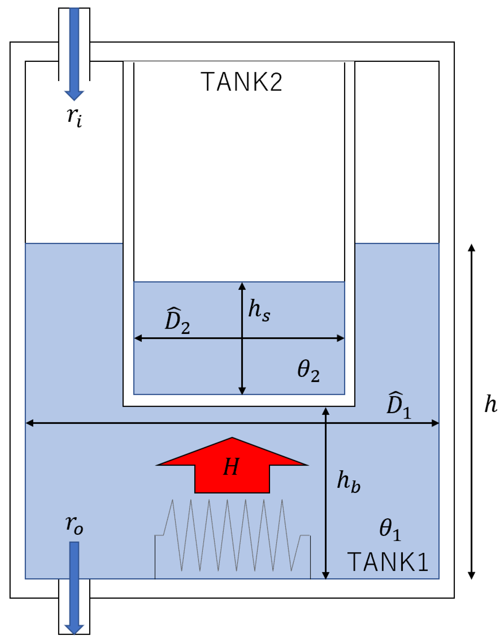
Figure 2. Tank heat balance.

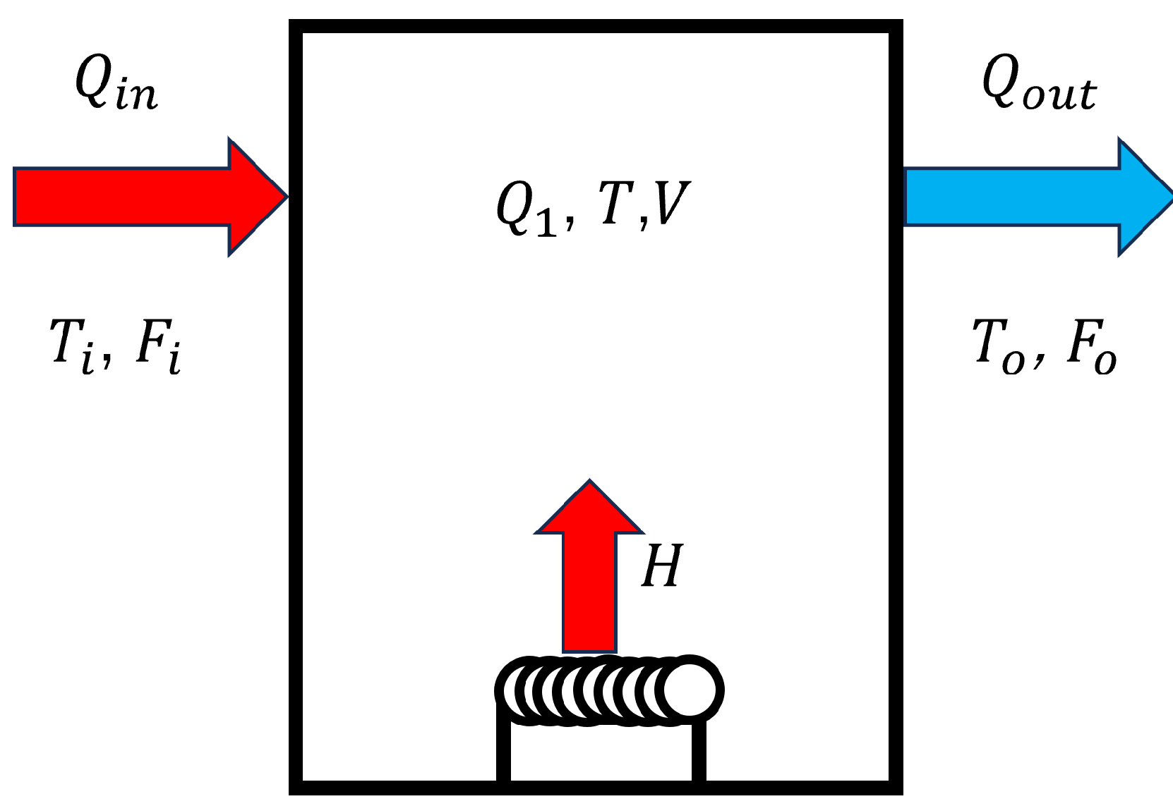
Figure 3. Proposed control system.

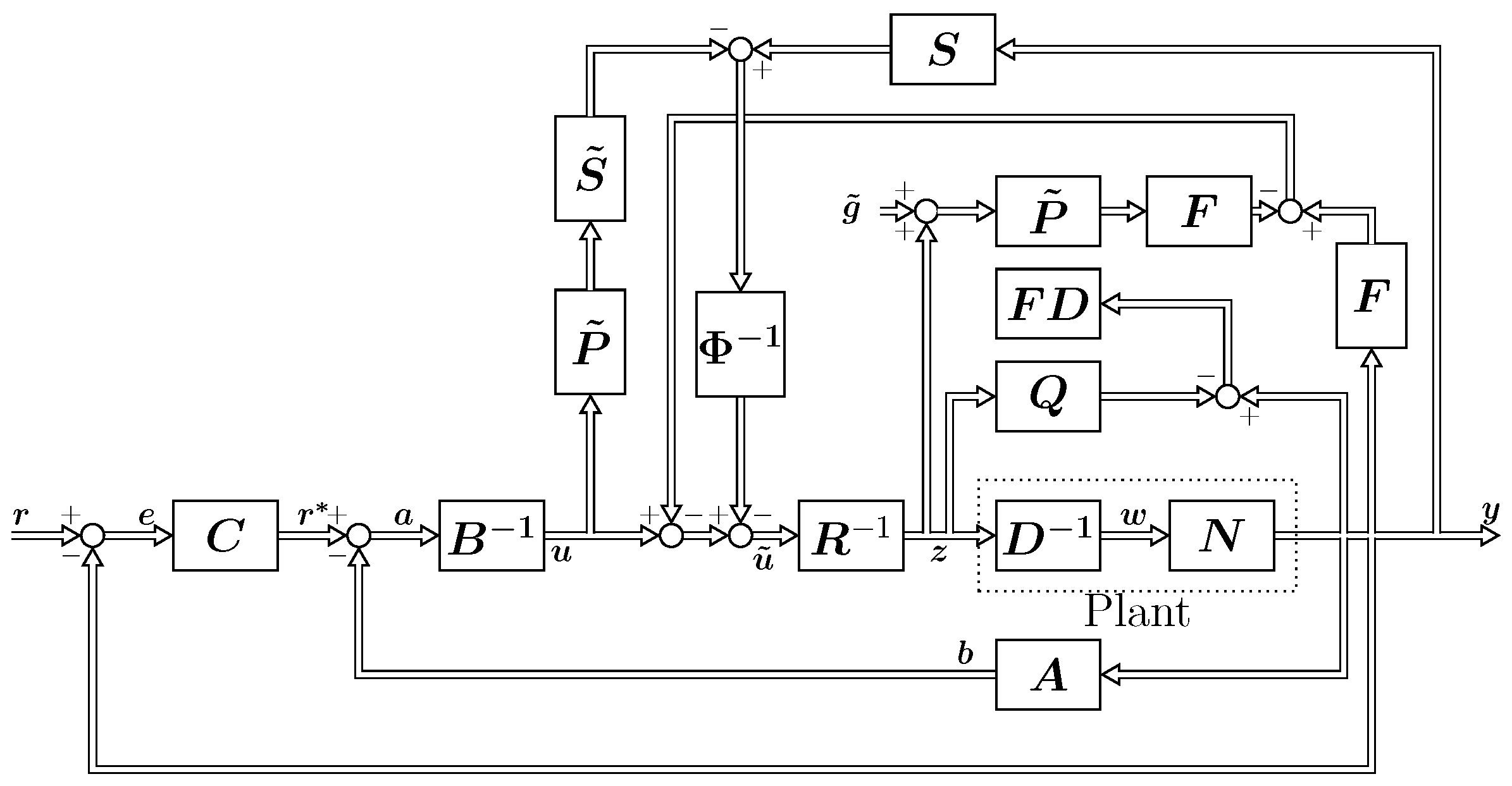
Figure 4. Uncertainty compensation.

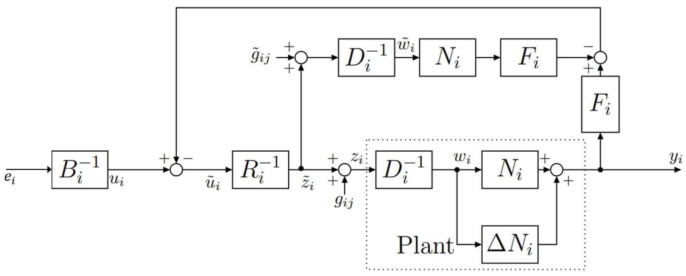
Figure 5. Elimination of coupling effects.

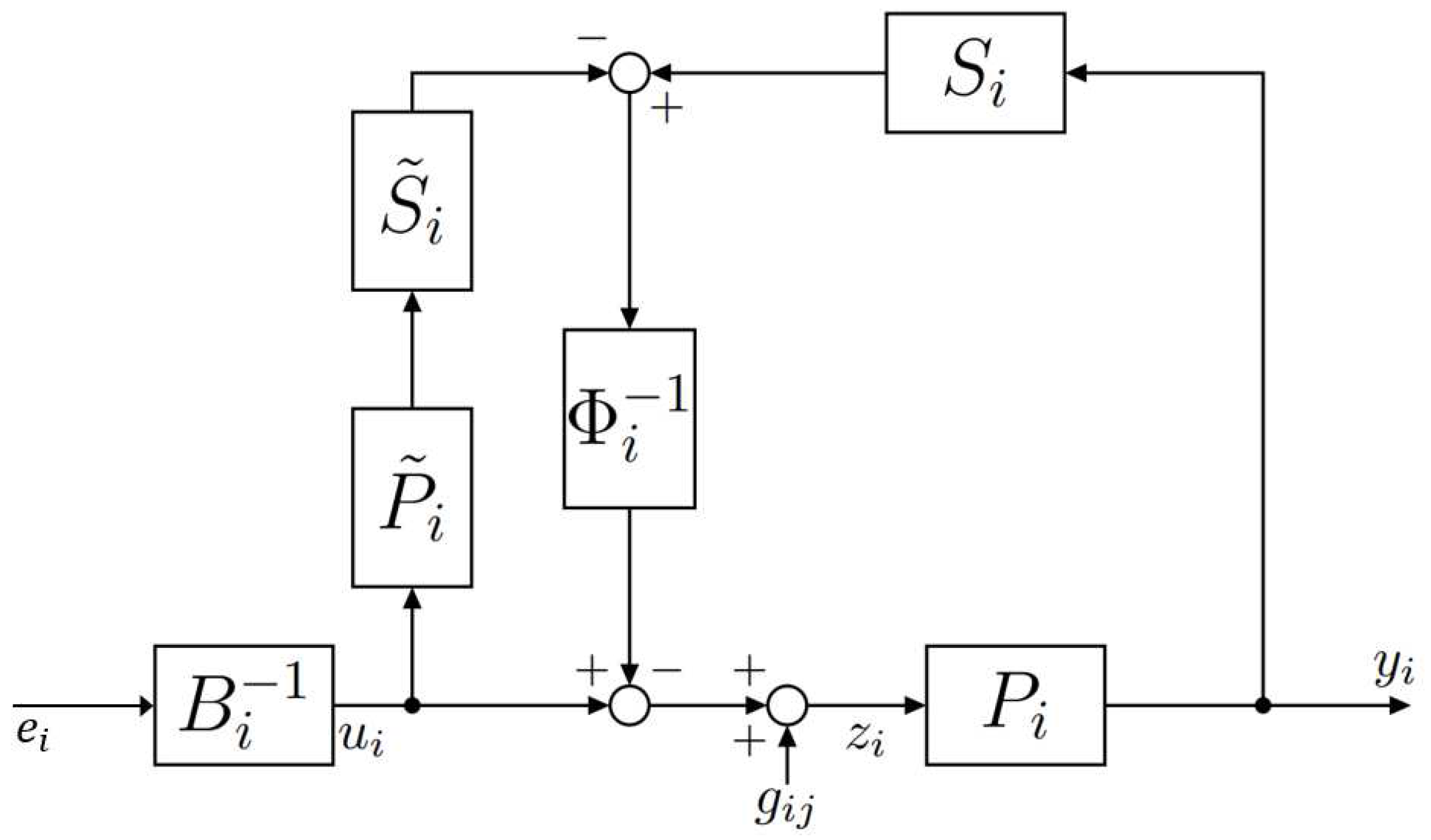
Figure 6. Details of the proposed control system.

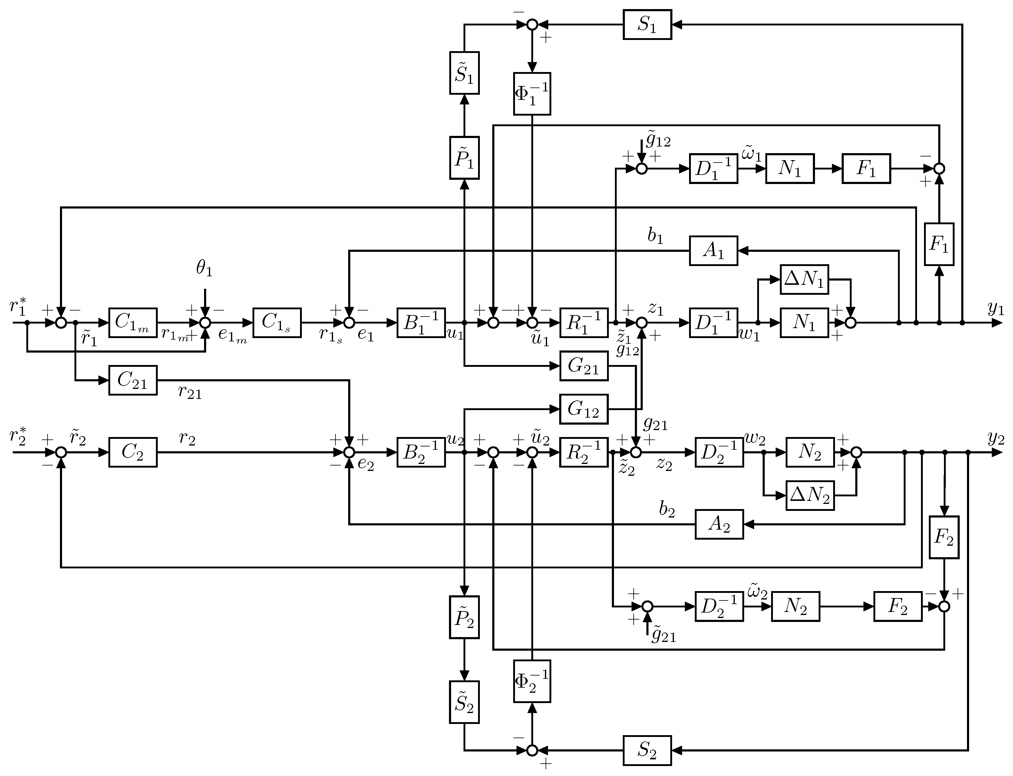
Figure 7. Simulation results: liquid temperature and heater output.

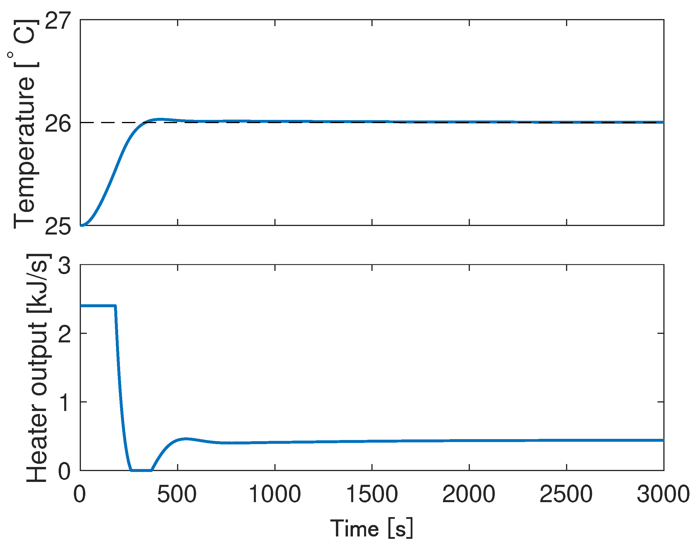
Figure 8. Simulation results: liquid level and input rate.

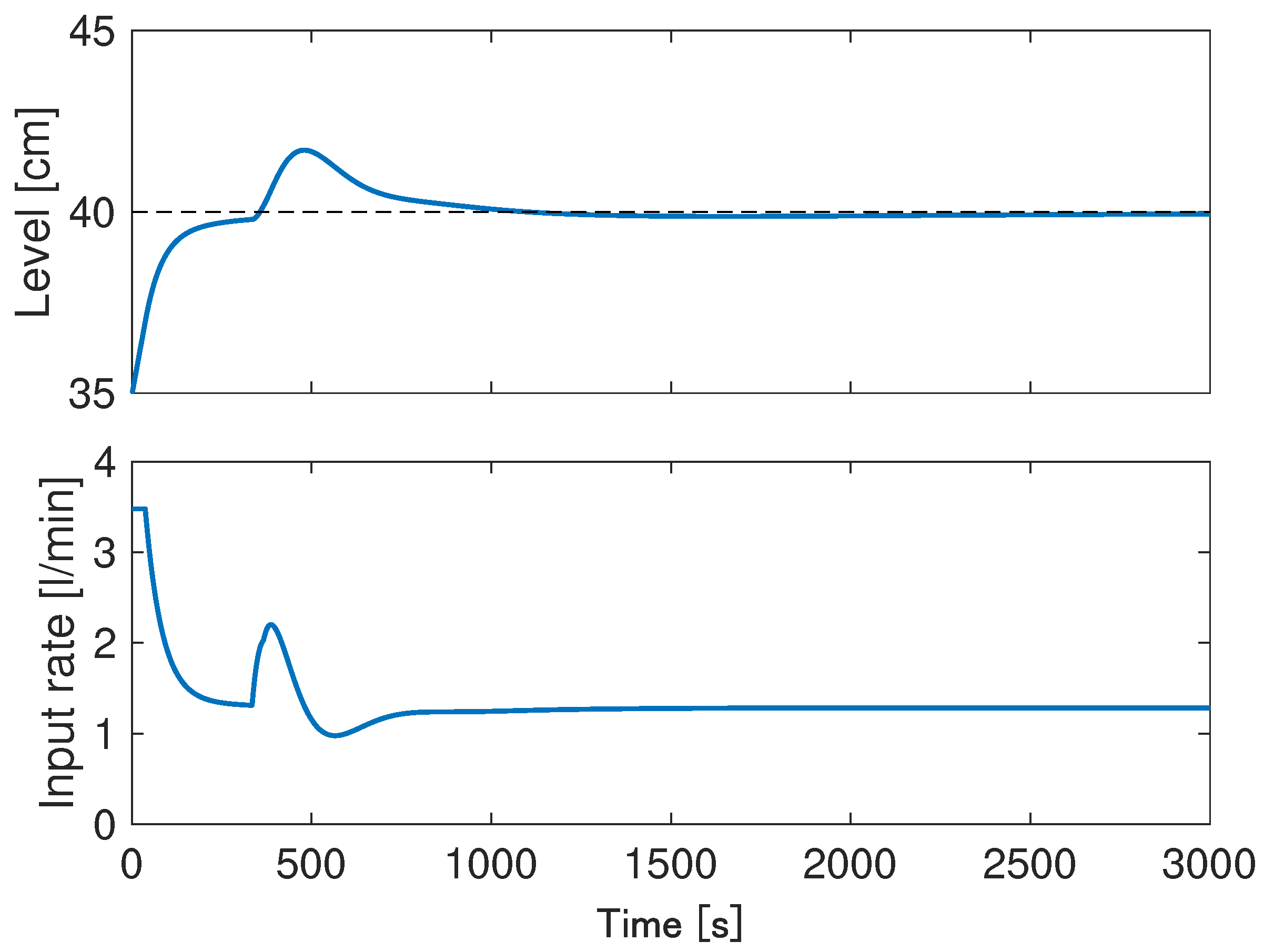
Figure 9. Experimental results: liquid temperature and heater output.

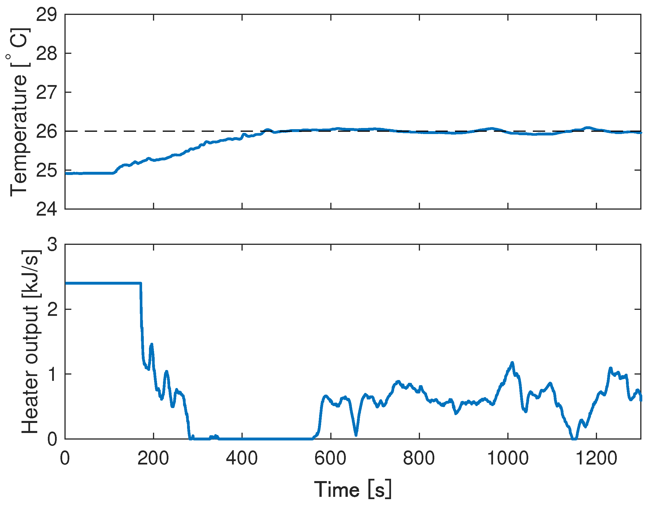
Figure 10. Experimental results: liquid level and input rate.

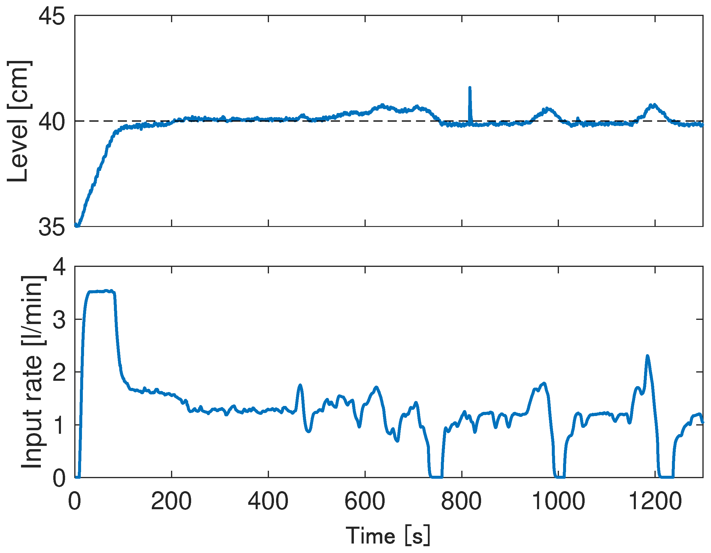
Table 1. Modeling parameters.

Parameter	Definition	Value
${\hat{D}}_{1}$	Inside diameter(TANK1)	32 cm
${\hat{D}}_{2}$	Inside diameter(TANK2)	11 cm
${\hat{D}}_{0}$	Inner diameter	4.0 cm
$δ$	Thickness of wall	2.0 cm
$h_{b}$	Distance between botttom	20 cm
$h_{s}$	Water level(TANK2)	35 cm
$α_{1}$	Heat transfer coefficient	$5.0 \times 10^{- 5}$ $kJ / (s \cdot {cm}^{2} \cdot^{\circ} C)$
$α_{2}$	Heat transfer coefficient	$1.5 \times 10^{- 4}$ $kJ / (s \cdot {cm}^{2} \cdot^{\circ} C)$
k	Thermal conductivity of TANK wall	$1.7 \times 10^{- 4}$ $kJ / (s \cdot cm \cdot^{\circ} C)$
$C_{TA}$	TANK1 wall heat capacity	47 $kJ /^{\circ} C$
$C_{2}$	Heat capacity of water in TANK2	$5.6$ $kJ /^{\circ} C$
$C_{TB}$	TANK2 wall heat capacity	10 $kJ /^{\circ} C$
$c_{w}$	Specific heat of water	$4.2 \times 10^{- 3}$ $kJ / (^{\circ} C \cdot g)$
$ρ_{w}$	Density of water	$1.0$ $g / {cm}^{3}$
g	acceleration of gravity	$9.8 \times 10^{2}$ $cm / s^{2}$
$θ_{1} i$	Temperature of influent liquid	18 $^{\circ} C$
$θ_{1}$	Liquid temperature(TANK1)	$^{\circ} C$
$θ_{2}$	Liquid temperature(TANK2)	$^{\circ} C$
${\hat{θ}}_{1}$	Outer wall temperature	$^{\circ} C$
${\hat{θ}}_{2}$	Inner wall temperature	$^{\circ} C$
h	Water level(TANK1)	$cm$
$C_{1}$	Heat capacity of water in TANK1	$kJ /^{\circ} C$
$r_{o}$	Liquid volume of effluent	$L / \min$
$r_{i}$	Liquid volume of influent	$L / \min$
H	Heat supplied by heater	$kJ / s$
$λ$	Thermal conductivity	$kJ / (s \cdot m \cdot^{\circ} C)$

Table 2. Simulation parameters.

Parameter	Definition	Value
	Simulation time	3500 $s$
	Sampling time	$1.0$ $s$
$r_{w}$	Target liquid level	40 $cm$
$r_{t}$	Target liquid temperature	26 $^{\circ} C$
$y_{w_{0}}$	Initial value	35 $cm$
$y_{t_{0}}$	Initial value	25 $^{\circ} C$
$K_{P_{t}}$	Proportional gain	3.0
$K_{I_{t}}$	Integral gain	0.0015
$K_{P_{w}}$	Proportional gain	1.0
$K_{I_{w}}$	Integral gain	0.003
$K_{P_{t w}}$	Proportional gain	50
$K_{I_{t w}}$	Integral gain	0.02
p	Differential factorial	$0.95$
q	Differential factorial	$1.05$
$q_{w}$	Differential factorial	$5 / 14$
$G_{1}$	Gain	$0.001$
$G_{2}$	Gain	$0.0005$
$ω_{1}$	Angular frequency	$π / 30$ $rad / s$
$ω_{2}$	Angular frequency	$3 π / 4$ $rad / s$

Table 3. Expriment parameters.

Parameter	Definition	Value
	Sampling time	$1.0$ $s$
	Outside temperature	22 $^{\circ} C$
$r_{w}$	Target liquid level	40 $cm$
$r_{t}$	Target liquid temperature	26 $^{\circ} C$
$y_{w_{0}}$	Initial value	35 $cm$
$y_{t_{0}}$	Initial value	25 $^{\circ} C$
$θ_{i}$	Inflow liquid temperature	20 $^{\circ} C$
$K_{P_{t}}$	Proportional gain	1.8
$K_{I_{t}}$	Integral gain	0.0024
$K_{P_{w}}$	Proportional gain	1.1
$K_{I_{w}}$	Integral gain	0.003
$K_{P_{t w}}$	Proportional gain	15
$K_{I_{t w}}$	Integral gain	0.001
p	Differential factorial	$1.1$
q	Differential factorial	$1.05$
$q_{w}$	Differential factorial	$5 / 14$
$G_{1}$	Gain	$0.001$
$G_{2}$	Gain	$0.0005$
$ω_{1}$	Angular frequency	$π / 30$ $rad / s$
$ω_{2}$	Angular frequency	$3 π / 4$ $rad / s$

Disclaimer/Publisher’s Note: The statements, opinions and data contained in all publications are solely those of the individual author(s) and contributor(s) and not of MDPI and/or the editor(s). MDPI and/or the editor(s) disclaim responsibility for any injury to people or property resulting from any ideas, methods, instructions or products referred to in the content.

© 2023 by the authors. Licensee MDPI, Basel, Switzerland. This article is an open access article distributed under the terms and conditions of the Creative Commons Attribution (CC BY) license (http://creativecommons.org/licenses/by/4.0/).

Copyright: This open access article is published under a Creative Commons CC BY 4.0 license, which permit the free download, distribution, and reuse, provided that the author and preprint are cited in any reuse.

Submitted:

05 December 2023

Posted:

06 December 2023

You are already at the latest version

Alerts

Abstract

Keywords:

Subject: Engineering - Electrical and Electronic Engineering

1. Introduction

2. Mathematical Preparation

2.1. Fractional Calculus

Grünwald

\begin{matrix} \frac{d f (t)}{d t} \equiv lim_{δ \to 0} \frac{f (t) - f (t - δ)}{δ} \end{matrix}

(1)

\begin{matrix} \frac{d^{2} f (t)}{d t^{2}} \equiv lim_{δ \to 0} \frac{f (t) - 2 f (t - δ) + f (t - 2 δ)}{δ} \end{matrix}

(2)

Generalizing as the derivative of integer nth order, Equation (3) is derived.

\frac{d^{n} f (t)}{d t^{n}} \equiv lim_{δ \to 0} \{δ^{- n} \sum_{k = 0}^{n} {(- 1)}^{k} (\binom{n}{k}) f (t - k δ)\}

(3)

When converted to the variable

δ = \frac{t - t_{0}}{N}

(\binom{n}{k}) = 0

when

j > n

, the Equation (3) can be transformed as in the Equation (4).

\frac{d^{n} f (t)}{d t^{n}} \equiv lim_{N \to \infty} ({(\frac{t - t_{0}}{N})}^{- n} \sum_{k = 0}^{N - 1} {(- 1)}^{k} (\binom{n}{k}) f (t - k \frac{t - t_{0}}{N}))

(4)

The binomial coefficient can be expressed as Equation (5) using the

Γ

function, since there is a relationship

Γ (n + 1) = n!

between the factorial

n!

and the

Γ

function.

\frac{d^{n} f (t)}{d t^{n}} \equiv lim_{N \to \infty} ({(\frac{t - t_{0}}{N})}^{- n} \sum_{k = 0}^{N - 1} \frac{Γ (k - n)}{Γ (k + 1) Γ (- n)} f (t - k \frac{t - t_{0}}{N}))

(5)

Since the

Γ

function is a function defined for real numbers, the derivative of Equation (5) can be extended from integer n to real number q. Therefore, we can derive the definition of

Grünwald

-Letnikov as shown in Equation (6).

\frac{d^{q} f (t)}{d t^{q}} \equiv lim_{N \to \infty} ({(\frac{t - t_{0}}{N})}^{- q} \sum_{k = 0}^{N - 1} \frac{Γ (k - q)}{Γ (k + 1) Γ (- q)} f (t - k \frac{t - t_{0}}{N}))

(6)

\frac{d^{q} f (t)}{d t^{q}} = Δ t^{- q} \sum_{k = 0}^{m - 1} \frac{Γ (k - q)}{Γ (k + 1) Γ (- q)} f (t - k Δ t)

(7)

2.2. Newmark- $β$ Method

β

method is used in this paper, which is a method for obtaining a solution by integrating differential equations at each small time interval and is also used in general differential equation analysis.

The algorithm of the Newmark-

β

method is shown below. First, the output

y (t)

and its first-, second-, and q-order derivatives at time t are described by using two parameters

γ

and

β

as follows.

\begin{matrix} y (t) & = Δ y (t) + y (t - 1) + Δ t \dot{y} (t - 1) + (0.5 - \frac{β}{γ}) Δ t^{2} \ddot{y} (t - 1) \end{matrix}

(8)

\begin{matrix} \dot{y} (t) & = \dot{y} (t - 1) + \frac{γ}{β Δ t} Δ y (t) \end{matrix}

(9)

\begin{matrix} \ddot{y} (t) & = \frac{1}{β Δ t^{2}} [Δ y (t) + (β - \frac{β}{γ}) Δ t^{2} \ddot{y} (t - 1)] \end{matrix}

(10)

\begin{matrix} \frac{d^{q} y (t)}{d t^{q}} & = \frac{1}{Γ (1 - q)} [I_{0} + Δ I_{t} + I_{t - 1}] \end{matrix}

(11)

where

Δ y (t)

I_{0}

Δ I_{t}

I_{t - 1}

is as follows.

\begin{matrix} Δ y (t) & = y (t) - y (t - 1) - Δ t \dot{y} (t - 1) - (0.5 - \frac{β}{γ}) Δ t^{2} \ddot{y} (t - 1) \end{matrix}

(12)

\begin{matrix} I_{0} & = \frac{y (0)}{t^{q}} \end{matrix}

(13)

\begin{matrix} Δ I_{t} & = \frac{Δ t^{- q}}{(1 - q) (2 - q)} (\frac{γ}{β}) [Δ y (t) + (2 - q) (\frac{β}{γ}) Δ t \dot{y} (t - 1)] \end{matrix}

(14)

\begin{matrix} I_{t - 1} & = \frac{Δ t}{2} [\frac{\dot{y} (0)}{t^{q}} + 2 \sum_{j = 1}^{t - 2} \frac{\dot{y} (j)}{{(t - j Δ t)}^{q}} + \frac{\dot{y} (t - 1)}{Δ t^{q}}] \end{matrix}

(15)

In this way, the fractional first-order differential equation can be replaced by the equation for the variable

Δ y

, which can be solved to obtain the output

y (t)

and its first-, second-, and q-order derivatives at time t, respectively. Depending on how

γ

and

β

are taken, the solution may diverge if the sampling time

Δ t

is not sufficiently small.

3. Modelling

3.1. Fractional Heat Exchange Process

q [J / s \cdot m^{2}]

and the thermal conductivity of the medium is

λ [J / s \cdot m^{2} \cdot^{\circ} C]

, heat conduction within the same material can be expressed by the Equation (16) to obtain the temperature distribution

θ (x)

of the medium at position x.

\begin{matrix} q = λ \frac{d θ (x)}{d x} \end{matrix}

(16)

Here, the thermal conductivity

λ

q [J / s \cdot m^{2}]

resulting from this is obtained from the heat transfer coefficient

α [J / s \cdot m^{2} \cdot K]

and the temperature difference between the objects

Δ θ [K]

by Equation (17).

\begin{matrix} q = α Δ θ \end{matrix}

(17)

The amount of heat transferred by heat conduction occurring within the side of the tank solid wall at a radial distance r from the center axis of TANK2,

Q_{s} [J / s]

, is expressed by the product of heat flux and heat transfer area using the Equation (18).

\begin{matrix} Q_{s} = 2 π r (h - (h_{b} + δ)) λ \frac{d θ (r)}{d r} \end{matrix}

(18)

Integrating Equation (18) with respect to temperature

θ

, the amount of heat transferred within the solid wall is expressed by the Equation (19), using the surface temperature of the solid wall

{\hat{θ}}_{2}

and

{\hat{θ}}_{1}

\begin{matrix} Q_{s} = \frac{2 π λ (h - (h_{b} + δ))}{ln (\frac{{\hat{D}}_{2} + 2 δ}{{\hat{D}}_{2}})} ({\hat{θ}}_{2} - {\hat{θ}}_{1}) \end{matrix}

(19)

Q_{s}

transferred from the liquid in TANK1 to the liquid in TANK2 by heat exchange at the tank side can be expressed by the Equation (20).

\begin{matrix} Q_{s} = \frac{π (h - (h_{b} + δ))}{\frac{1}{α_{1} ({\hat{D}}_{2} + 2 δ)} + \frac{1}{2 k} ln (\frac{{\hat{D}}_{2} + 2 δ}{{\hat{D}}_{2}}) + \frac{1}{α_{2} {\hat{D}}_{2}}} (θ_{1} - θ_{2}) \end{matrix}

(20)

Similarly, the heat quantity

Q_{b} [J / s]

transferred from the liquid in TANK1 to the liquid in TANK2 by heat exchange at the tank bottom is expressed by the Equation (21).

\begin{matrix} Q_{b} = \frac{π {\hat{D}}_{2}^{2}}{4 (\frac{δ}{λ} + \frac{1}{α_{1}} + \frac{1}{α_{2}})} (θ_{1} - θ_{2}) \end{matrix}

(21)

From Equations (20) and (21), the heat quantity

Q_{a} [J / s]

transferred from the liquid in TANK1 to the liquid in TANK2 due to the heat exchange that occurs throughout the tank is expressed by the Equation (22).

\begin{matrix} Q_{a} = Q_{s} + Q_{b} = k (θ_{1} - θ_{2}) \end{matrix}

(22)

k is expressed in Equation (23).

\begin{matrix} k & = \frac{π (h - (h_{b} + δ))}{\frac{1}{α_{1} ({\hat{D}}_{2} + 2 δ)} + \frac{1}{2 k} ln (\frac{{\hat{D}}_{2} + 2 δ}{{\hat{D}}_{2}}) + \frac{1}{α_{2} {\hat{D}}_{2}}} + \frac{π {\hat{D}}_{2}^{2}}{4 (\frac{δ}{λ} + \frac{1}{α_{1}} + \frac{1}{α_{2}})} \end{matrix}

(23)

Next, the concept of the heat balance of the tank is explained. where

Q_{i}, Q_{o} [J]

is heat value,

H [J]

is heater output,

T_{i}, T_{o} [° C]

is liquid temperature,

F_{i}, F_{o} [m^{3} / s]

is flow rate,

V [m^{3}]

is liquid volume,

c_{p} [kJ / kg \cdot K]

is the specific heat and

ρ [kg / m^{3}]

\begin{matrix} \frac{d Q_{1}}{d t} = Q_{i n} - Q_{o u t} + H \end{matrix}

(24)

The heat quantity Q can be expressed as

Q = ρ c_{p} V T

, and is substituted into the Equation (24).

\begin{matrix} ρ c_{p} \frac{d {V T}}{d t} = F_{i} ρ c_{p} T_{i} - F_{o} ρ c_{p} T_{o} + H \end{matrix}

(25)

Equation (25) can be transformed as in Equation (26), because in this paper we are considering the case where the liquid volume in the tank changes for TANK1.

\begin{matrix} V \frac{d T}{d t} = F_{i} T_{i} - F_{o} T_{o} + \frac{1}{ρ c_{p}} H - T \frac{d V}{d t} \end{matrix}

(26)

\begin{matrix} { & \begin{matrix} C_{1} \frac{d θ_{1}}{d t} = ρ_{w} c_{w} r_{i} θ_{1 i} - ρ_{w} c_{w} r_{0} θ_{1} + H \\ (27) & + k (θ_{2} - θ_{1}) - χ_{q} \frac{d^{q} θ_{1}}{d t^{q}} \\ - ρ_{w} c_{w} θ_{1} \frac{d V}{d t} \\ (28) & C_{2} \frac{d θ_{2}}{d t} = k (θ_{1} - θ_{2}) - χ_{p} \frac{d^{p} θ_{2}}{d t^{p}} \end{matrix} \end{matrix}

χ_{q}

and

χ_{p}

is expressed in Equations (29) and (30).

\begin{matrix} χ_{q} = \frac{d^{1 - q} C_{T A}}{d t^{1 - q}} \end{matrix}

(29)

\begin{matrix} χ_{p} = \frac{d^{1 - p} C_{T B}}{d t^{1 - p}} \end{matrix}

(30)

From Equations (27) and (28), the differential Equation (31) is derived.

\begin{matrix} C_{1} C_{2} B \frac{d^{2} θ_{2}}{d t^{2}} + (C_{1} + C_{2} + ρ_{w} c_{w} r_{i} C_{2} B) \frac{d θ_{2}}{d t} + ρ_{w} c_{w} r_{i} θ_{2} + (ρ_{w} c_{w} r_{i} B χ_{p} + χ_{p}) \frac{d^{p} θ_{2}}{d t^{p}} \\ + χ_{q} \frac{d^{q} θ_{2}}{d t^{q}} + C_{1} χ_{p} B \frac{d^{p + 1} θ_{2}}{d t^{p + 1}} + C_{2} χ_{q} B \frac{d^{q + 1} θ_{2}}{d t^{q + 1}} + χ_{q} χ_{p} B \frac{d^{p + q} θ_{2}}{d t^{p + q}} = ρ_{w} c_{w} r_{i} θ_{1 i} + H \end{matrix}

(31)

Solving Equation (31) for

θ_{2}

yields a model of the heat exchange process. The coefficients

χ_{q}

and

χ_{p}

are determined by considering the dimension of the model. Specifically, the dimension of

χ_{q}

[J / K \cdot s^{1 - q}]

and that of

χ_{p}

[J / K \cdot s^{1 - p}]

. This confirms that the dimensions of the left and right sides of the heat balance equation match.

3.2. Fractional Liquid Process

The area A of the liquid surface of TANK1 and the area a of the outlet at the bottom of TANK1 are expressed by Equations (32) and (33).

\begin{matrix} A & = \frac{π}{4} [{\hat{D}}_{1}^{2} - {({\hat{D}}_{2} + 2 δ)}^{2}] \end{matrix}

(32)

\begin{matrix} a & = \frac{π {\hat{D}}_{0}^{2}}{4} \end{matrix}

(33)

Letting the inflow into TANK1 be

r_{i} (t)

and the outflow be

r_{o} (t)

, the Equation (34) is obtained for the time variation of the liquid level

h (t)

in TANK1.

A \dot{h} (t) = r_{i} (t) - r_{o} (t)

(34)

The inflow

r_{i} (t)

is the control input and is observable. The outflow

r_{o} (t)

is expressed as the product of the cross-sectional area of the outlet and the velocity of the outflow. The velocity

v (t)

at which the liquid in the container flows out through the small hole is obtained from Torricelli’s theorem and is expressed as in the Equation (35).

v (t) = \sqrt{2 g h (t)}

(35)

Therefore, the outflow from TANK1 is obtained as in Equation (36).

r_{o} (t) = a \sqrt{2 g h (t)}

(36)

From Equations (34), (35) and (36), we obtain Equation (37) as the model equation for the liquid level system.

\dot{h} (t) = \frac{1}{A} r_{i} (t) - \frac{a}{A} \sqrt{2 g h (t)}

(37)

Here, the inflow rate

r_{i} (t)

has a role as a cooling input for liquid temperature control in addition to its role as an input for liquid level control in the dual tank device used in this paper. Therefore, the inflow rate

r_{i} (t)

includes the interference from the heater in addition to the input

r_{i}^{'} (t)

from the pump, and is considered to be expressed by Equation (38).

\begin{matrix} r_{i} (t) = r_{i}^{'} (t) + \frac{1}{ρ c_{w} (θ_{1} - θ_{i})} H \end{matrix}

(38)

\begin{matrix} D^{q_{w}} (G_{1} sin (ω_{1} t) + G_{2} cos (ω_{2} t)) \\ ≃ & {(G_{1} ω_{1})}^{q_{w}} [sin (ω_{1} t + \frac{π q_{w}}{2}) + \frac{{(ω_{1} t)}^{- 1 - q_{w}}}{Γ (- q_{w})} + \frac{{(ω_{1} t)}^{- 3 - q_{w}}}{Γ (- q_{w} - 2)}] \\ + & {(G_{2} ω_{2})}^{q_{w}} [cos (ω_{2} t + \frac{π q_{w}}{2}) + \frac{{(ω_{2} t)}^{- 2 - q_{w}}}{Γ (- q_{w} - 1)} + \frac{{(ω_{2} t)}^{- 4 - q_{w}}}{Γ (- q - 3)}] \end{matrix}

(39)

4. Multivariable Fractional-Order Nonlinear Control Feedback System Design

N = (N_{1}, N_{2})

D = (D_{1}, D_{2})

is the plant and

A = (A_{1}, A_{2})

B = (B_{1}, B_{2})

S = (S_{1}, S_{2})

F = (F_{1}, F_{2})

\tilde{P} = ({\tilde{P}}_{1}, {\tilde{P}}_{2})

Φ = (Φ_{1}, Φ_{2})

R = (R_{1}, R_{2})

C = (C_{1}, C_{2})

is the controller.

4.1. Fractional Liquid Temperature Control Design

Transforming the model equation derived in the previous section, we obtain the plant

P_{1} : Z_{1} \to Y_{1}

. The operator

N_{1}, D_{1}^{- 1}

satisfying the right decomposition

P_{1} (z_{1}) (t) = N_{1} D_{1}^{- 1} (z_{1}) (t)

for the plant

P_{1}

can be designed as in Equations (40) and (41).

\begin{matrix} N_{1} : \{\begin{matrix} C_{1} C_{2} B \frac{d^{2} x_{1} (t)}{d t^{2}} + (ρ_{w} c_{w} r_{i} + k) B χ_{p} \frac{d^{p} x_{1} (t)}{d t^{p}} \\ + (C_{1} + C_{2} + C_{2} B ρ_{w} c_{w} r_{i}) \frac{d x_{1} (t)}{d t} + ρ_{w} c_{w} r_{i} x_{1} (t) \\ + χ_{q} \frac{d^{q} x_{1} (t)}{d t^{q}} + C_{1} χ_{p} B \frac{d^{p + 1} x_{1} (t)}{d t^{p + 1}} + C_{2} χ_{q} B \frac{d^{q + 1} x_{1} (t)}{d t^{q + 1}} \\ + χ_{q} χ_{p} B \frac{d^{p + q} x_{1} (t)}{d t^{p + q}} = w_{1} (t) \\ θ_{2} (t) = x_{1} (t) \end{matrix} \end{matrix}

(40)

\begin{matrix} D_{1} : z_{1} (t) = I (w_{1} (t)) \end{matrix}

(41)

Next, design controllers

A_{1}, B_{1}

that satisfy the Bezoo equality

A_{1} N_{1} + B_{1} D_{1} = M

. Let M be a unimodular operator. When

A_{1}, B_{1}

K_{t}

is shown in Equation (1).

\begin{matrix} A_{1} : b_{1} (t) & = (1 - K_{t}) (C_{1} C_{2} B \frac{d^{2} θ_{2} (t)}{d t^{2}} + (C_{1} + C_{2} + C_{2} B ρ_{w} c_{w} r_{i}) \frac{d θ_{2} (t)}{d t} \end{matrix}

\begin{matrix} + & ρ_{w} c_{w} r_{i} θ_{2} (t) + (ρ_{w} c_{w} r_{i} + k) B χ_{p} \frac{d^{p} θ_{2} (t)}{d t^{p}} + χ_{q} \frac{d^{q} θ_{2} (t)}{d t^{q}} + C_{1} χ_{p} B \frac{d^{p + 1} θ_{2} (t)}{d t^{p + 1}} \\ + & C_{2} χ_{q} B \frac{d^{q + 1} θ_{2} (t)}{d t^{q + 1}} + χ_{q} χ_{p} B \frac{d^{p + q} θ_{2} (t)}{d t^{p + q}}) \end{matrix}

(42)

\begin{matrix} B_{1} : e_{1} (t) & = K_{t} u_{1} (t) \end{matrix}

(43)

A tracking compensator was designed to compensate for tracking performance. In Figure 3,

C_{1_{m}}

C_{21}

is a follow-up compensator that operates with the difference between TANK2 temperature

θ_{2}

and target temperature as input and a controller that calculates the amount of liquid pumped based on the difference in liquid temperature, and

C_{1_{s}}

is a controller that operates with TANK1 temperature

θ_{1}

as feedback.

C_{1_{s}}

is a follow-up compensator that operates with the TANK1 temperature

θ_{1}

as feedback.

\begin{matrix} C_{1_{m}} : r_{1_{m}} (t) = K_{P_{t 1}} {\tilde{r}}_{1} (t) + K_{I_{t 1}} \int_{t_{0}}^{t} {\tilde{r}}_{1} (τ) d τ \end{matrix}

(44)

\begin{matrix} C_{1_{s}} : r_{1_{s}} (t) = K_{P_{t 2}} e_{1_{m}} (t) + K_{I_{t 2}} \int_{t_{0}}^{t} e_{1_{m}} (τ) d τ \end{matrix}

(45)

\begin{matrix} C_{21} : r_{21} (t) = K_{P_{t w}} {\tilde{r}}_{1} (t) + K_{I_{t w}} \int_{t_{0}}^{t} {\tilde{r}}_{1} (τ) d τ \end{matrix}

(46)

4.2. Fractional Liquid Level Control Design

Similar to the liquid temperature control design, the right-hand decomposition

N_{2}, D_{2}

and stabilizing compensators

A_{2}, B_{2}

of the plant are designed as follows. where

K_{w}

is the design coefficient.

\begin{matrix} N_{2} : \{\begin{matrix} {\dot{x}}_{2} (t) = w_{2} (t) - \frac{a}{A} \sqrt{2 g x_{2} (t)} \\ y_{2} (t) = x_{2} (t) \end{matrix} \end{matrix}

(47)

\begin{matrix} Δ N_{2} : D^{q} (G_{1} sin (ω_{1} t) + G_{2} cos (ω_{2} t)) \end{matrix}

(48)

\begin{matrix} D_{2} : u_{2} (t) = A w_{2} (t) \end{matrix}

(49)

\begin{matrix} A_{2} : b_{2} (t) = (1 - K_{w}) ({\dot{y}}_{2} (t) + \frac{a}{A} \sqrt{2 g y_{2} (t)}) \end{matrix}

(50)

\begin{matrix} B_{2} : e_{2} (t) = \frac{K_{p}}{A} u_{2} (t) \end{matrix}

(51)

where for the signal

z_{2} (t)

appearing at the plant

N_{2}

D_{2}

, the interference from the heater shown during modeling is included, in addition to the liquid level control input

u_{2} (t)

. The tracking compensator is designed in the same way.

\begin{matrix} C_{2} : r_{2} (t) = K_{P w} {\tilde{r}}_{2} (t) + K_{I w} \int_{t_{0}}^{t} {\tilde{r}}_{2} (τ) d τ \end{matrix}

(52)

4.3. Interference Design

G_{12} : U_{2} \to U_{1}

, which gives the Equation (53).

\begin{matrix} G_{12} (u_{2} (t)) = ρ_{w} c_{w} θ_{1 i} u_{2} (t) \end{matrix}

(53)

Next, the liquid level process is designed in the same way. In the liquid temperature control method used in this paper, the controller

C_{21}

G_{21} : U_{1} \to U_{2}

, which gives the Equation (54).

\begin{matrix} G_{21} (u_{1} (t)) = \frac{u_{1} (t)}{ρ_{w} c_{w} (θ_{1} - θ_{1 i})} \end{matrix}

(54)

4.4. Uncertainty Compensation Design

The feedback system of uncertainty compensation is shown in Figure 4.

The actual process, a dual tank device, has uncertainties that are not included in the model. The process

P_{i} + Δ P_{i}

including this uncertainty is expressed as in Equation (55).

\begin{matrix} P_{i} + Δ P_{i} = (N_{i} + Δ N_{i}) D_{i}^{- 1} \end{matrix}

(55)

As an example, consider the case where

i = 1

j = 2

. In this case, the signal

{\tilde{u}}_{1}

can be expressed as in Equation (56). where

{\tilde{g}}_{12}

is the ideal interference without uncertainty.

\begin{matrix} {\tilde{u}}_{1} = u_{1} - F_{1} (y_{1}) + F_{1} N_{1} ({\tilde{ω}}_{1}) \\ = R_{1} (D_{1} ({\tilde{ω}}_{1}) - {\tilde{g}}_{12}) \end{matrix}

(56)

R_{1}

is designed as a linear operator, Equation (56) is expressed as in Equation (57).

\begin{matrix} R_{1} D_{1} ({\tilde{ω}}_{1}) - F_{1} N_{1} ({\tilde{ω}}_{1}) = u_{1} - F_{1} (y_{1}) + R_{1} ({\tilde{g}}_{12}) \end{matrix}

(57)

The signal

{\tilde{ω}}_{1}

can be transformed as in Equation (58) since

D_{1}^{- 1}

is a linear operator.

\begin{matrix} {\tilde{ω}}_{1} = D_{1}^{- 1} ({\tilde{z}}_{1} + {\tilde{g}}_{12}) = D_{1}^{- 1} ({\tilde{z}}_{1}) + D_{1}^{- 1} ({\tilde{g}}_{12}) \end{matrix}

(58)

Substituting the signal

{\tilde{ω}}_{1}

into the Equation (56) and transforming it, we obtain the Equation (59).

\begin{matrix} R_{1} ({\tilde{z}}_{1}) + R_{1} ({\tilde{g}}_{12}) - F_{1} P_{1} ({\tilde{z}}_{1}) - F_{1} P_{1} ({\tilde{g}}_{12}) \\ = u_{1} - F_{1} (y_{1}) + R_{1} ({\tilde{g}}_{12}) \end{matrix}

(59)

Here, by designing

F_{1} P_{1} = I

and

R_{1} = I

, it is expressed as in Equation (60). where I is an identity map.

\begin{matrix} u_{1} + {\tilde{g}}_{12} = F_{1} (y_{1}) \end{matrix}

(60)

Thus, the ideal output and the output with uncertainty are equal, and the uncertainty can be compensated.

4.5. Coupling Effects Elimination Design

The control system that eliminates coupling effects is shown in Figure 5.

In this section, we consider the case

i = 1, j = 2

. When controlling liquid temperature and liquid level simultaneously, there is mutual interference in terms of the heat supplied and the amount of liquid pumped. In Figure 3,

z_{1} (t)

is represented by the Equation (61).

\begin{matrix} z_{1} (t) = & u_{1} + g_{12} - ϕ_{1}^{- 1} S_{1} P (z_{1}) + ϕ_{1}^{- 1} {\tilde{S}}_{1} {\tilde{P}}_{1} (u_{1}) \end{matrix}

(61)

where

ϕ_{1}

and

ϕ_{1}^{- 1}

can be transformed as in Equation (62) when designed as linear operators.

\begin{matrix} ϕ_{1}^{- 1} (ϕ_{1} + S_{1} P_{1}) (z_{1}) = g_{12} + ϕ_{1}^{- 1} (ϕ_{1} + {\tilde{S}}_{1} {\tilde{P}}_{1}) (u_{1}) \end{matrix}

(62)

Therefore, the controller is designed to satisfy the relationship such that the Equation (62). Each operator is designed with

S_{1} = I

and

ϕ^{- 1} (α_{1}) (t) = \frac{1}{n} α_{1}

. where

\frac{1}{n} α_{1}

is the bounded signal and n is the design parameter. By

ϕ_{1}^{- 1}

and

ϕ_{1}

, we have Equation (63).

\begin{matrix} z_{1} \to u_{1} \end{matrix}

(63)

Equation (63) shows that the input signal

Z_{1}

and the output

U_{1}

of operator

B_{1}^{- 1}

are equal, thus eliminating coupling effects.

4.6. Control System Design Details

Finally, the details of the control system design used in this paper are shown in Figure 6. For plants

D, N, Δ N

and controllers

A, B, R, C, F, S, \tilde{S}, \tilde{P}, Φ

in the control system, subscripts of 1 are related to the liquid temperature control system and those of 2 to the liquid level control system.

C_{21}

refers to a controller that calculates the amount of liquid pumped based on the difference in liquid temperature,

G_{12}, G_{21}

refers to interference between the liquid temperature control system and the liquid level control system.

5. Results and Discussion

5.1. Simulation Results

θ_{2}

was set, and the overshoot was reduced by pumping liquid. From Figure 7 and Figure 8, it can be seen that the liquid flow rate increases when

θ_{2}

exceeds the target value and the cooling operation is performed. Finally, it can be seen that the liquid temperature and liquid level follow the target values.

5.2. Exprimental Results

^{\circ}

C and 26

^{\circ}

θ_{2}

exceeds the target value in the experiment as well. When a slight overshoot occurs for

θ_{2}

, it can be confirmed that the overshoot is reduced by pumping liquid. Both the liquid temperature and the liquid level are finally able to follow the target values.

6. Conclusions

Author Contributions

Funding

This research received no external funding.

Institutional Review Board Statement

Not applicable.

Informed Consent Statement

Not applicable.

Data Availability Statement

Data is contained within the article.

Conflicts of Interest

The authors declare no conflict of interest.

References

Deng, M.; Iwai, Z.; Mizumoto, I. Robust parallel compensator design for output feedback stabilization of plants with structured uncertainty. Systems Control Letters 1999, 36, 193–198. [Google Scholar] [CrossRef]
Shah, S.L.; Iwai, Z.; Mizumoto, I.; Deng, M. Simple adaptive control of processes with time-delay. Journal of Process Control 1997, 7, 439–449. [Google Scholar] [CrossRef]
Matsumoto, K.; Saito, D.; Wakui, S. Comparison of Connection Methods of One-axis Tracking Filters and Implementation for Pneumatic Anti-Vibration Apparatus. In Proceedings of the 2018 International Conference on Advanced Mechatronic Systems, Zhengzhou, China, 29 August-2 September 2018. [Google Scholar]
Ishii, H.; Wakui, S. Performance improvement of PDD2 compensator embedded in position control for pneumatic stage. In Proceedings of the 2019 International Conference on Advanced Mechatronic Systems, Kusatsu, Japan, 26-28 August 2019. [Google Scholar]
Patra, A.K.; Nanda, A. Automated micro insulin dispenser system based on the model predictive control algorithm. International Journal of Advanced Mechatronic Systems 2020, 8, 144–154. [Google Scholar] [CrossRef]
Wen, S.; Liang, T.; Wang, P. Adaptive position estimation and control for permanent magnet synchronous motor. In Proceedings of the 2018 International Conference on Advanced Mechatronic Systems, Zhengzhou, China, 29 August-2 September 2018. [Google Scholar]
Shafieenejad, I. Novel method for bang-bang optimal control of starship soft landing. International Journal of Advanced Mechatronic Systems 2023, 10, 146–155. [Google Scholar] [CrossRef]
Wang, C.; Man, Z.; Jin, J.; Ye, W. Hash-Based Convolutional Deep-thinking Pattern Classifier. In Proceedings of the 2023 International Conference on Advanced Mechatronic Systems, Melbourne, Australia, 4-7 September 2023. [Google Scholar]
Cheng, W.; Liu, T.; Liang, S. Temperatrue Control of Microwave Heating System by Adaptive Dynamic Programming. In Proceedings of the 2020 International Conference on Advanced Mechatronic Systems, Hanoi, Vietnam, 10-13 December 2020. [Google Scholar]
Rsetam, K.; Cao, Z.; Man, Z. Design of Robust Terminal Sliding Mode Control for Underactuated Flexible Joint Robot. IEEE Transactions on Systems, Man, and Cybernetics: Systems 2022, 52, 4272–4285. [Google Scholar] [CrossRef]
Man, Z.; Paplinski, A.P.; Wu, H.R. A robust MIMO terminal sliding mode control scheme for rigid robotic manipulators. IEEE Transactions on Automatic Control 1994, 39, 2464–2469. [Google Scholar]
Wang, H.; Man, Z.; Kong, H.; Zhao, Y.; Yu, M.; Cao, Z.; Zheng, J.; Do, M.T. Design and Implementation of Adaptive Terminal Sliding-Mode Control on a Steer-by-Wire Equipped Road Vehicle. IEEE Transactions on Industrial Electronics 2016, 63, 5774–5785. [Google Scholar] [CrossRef]
Yu, X.; Man, Z. Model reference adaptive control systems with terminal sliding modes. International Journal of Control 1996, 64, 1165–1176. [Google Scholar] [CrossRef]
Chen, J.; Qian, D. Three controllers via 2nd-order sliding mode for leader-following formation control of multi-robot systems. International Journal of Advanced Mechatronic Systems 2021, 9, 85–101. [Google Scholar] [CrossRef]
Deng, M. Operator-based nonlinear control systems: Design and applications; John Wiley & Sons: Hoboken, New Jersey, USA, 2014; pp. 5–26. [Google Scholar]
Chen, G.; Han, Z. Robust right coprime factorization and robust stabilization of nonlinear feedback control systems. IEEE Transactions on Automatic Control 1998, 43, 1505–1509. [Google Scholar] [CrossRef]
Gao, X.; Yang, Q.; Zhang, J. Multi-objective optimisation for operator-based robust nonlinear control design for wireless power transfer systems. International Journal of Advanced Mechatronic Systems 2022, 9, 203–210. [Google Scholar] [CrossRef]
Bu, N.; Zhang, Y.; Li, X. Robust tracking control for uncertain micro-hand actuator with Prandtl-Ishlinskii hysteresis. International Journal of Robust and Nonlinear Control 2023, 33, 9391–9405. [Google Scholar] [CrossRef]
Bu, N.; Liu, H.; Li, W. Robust passive tracking control for an uncertain soft actuator using robust right coprime factorization. International Journal of Robust and Nonlinear Control 2021, 31, 6810–6825. [Google Scholar] [CrossRef]
Bu, N.; Wang, X. Swing-up design of double inverted pendulum by using passive control method based on operator theory. International Journal of Advanced Mechatronic Systems 2023, 10, 1–7. [Google Scholar] [CrossRef]
Wang, A.; Deng, M. Robust nonlinear multivariable tracking control design to a manipulator with unknown uncertainties using operator-based robust right coprime factorization. Transactions of the Institute of Measurement and Control 2013, 35, 788–797. [Google Scholar] [CrossRef]
Deng, M.; Inoue, A.; Goto, S. Operator based thermal control of an aluminum plate with a peltier device. International Journal of Innovative Computing, Information and Control 2008, 4, 3219–3229. [Google Scholar]
Furukawa, K.; Deng, M. Operator based fault detection and compensation design of an unknown multivariable tank process. In Proceedings of the 2013 International Conference on Advanced Mechatronic Systems, Luoyang, China, 25–27 September 2013. [Google Scholar]
Keith, B.O.; Jerome, S. The Fractional Calculus; Dover Publications: Mineola, New York, USA, 2006; pp. 107–117. [Google Scholar]
Das, S. Functional Fractional Calculus; Springer: Berlin, Heidelberg, Germany, 2011; pp. 149–152. [Google Scholar]

Figure 1. Cross section of tank device.

Figure 2. Tank heat balance.

Figure 3. Proposed control system.

Figure 4. Uncertainty compensation.

Figure 5. Elimination of coupling effects.

Figure 6. Details of the proposed control system.

Figure 7. Simulation results: liquid temperature and heater output.

Figure 8. Simulation results: liquid level and input rate.

Figure 9. Experimental results: liquid temperature and heater output.

Figure 10. Experimental results: liquid level and input rate.

Table 1. Modeling parameters.

Parameter	Definition	Value
${\hat{D}}_{1}$	Inside diameter(TANK1)	32 cm
${\hat{D}}_{2}$	Inside diameter(TANK2)	11 cm
${\hat{D}}_{0}$	Inner diameter	4.0 cm
$δ$	Thickness of wall	2.0 cm
$h_{b}$	Distance between botttom	20 cm
$h_{s}$	Water level(TANK2)	35 cm
$α_{1}$	Heat transfer coefficient	$5.0 \times 10^{- 5}$ $kJ / (s \cdot {cm}^{2} \cdot^{\circ} C)$
$α_{2}$	Heat transfer coefficient	$1.5 \times 10^{- 4}$ $kJ / (s \cdot {cm}^{2} \cdot^{\circ} C)$
k	Thermal conductivity of TANK wall	$1.7 \times 10^{- 4}$ $kJ / (s \cdot cm \cdot^{\circ} C)$
$C_{TA}$	TANK1 wall heat capacity	47 $kJ /^{\circ} C$
$C_{2}$	Heat capacity of water in TANK2	$5.6$ $kJ /^{\circ} C$
$C_{TB}$	TANK2 wall heat capacity	10 $kJ /^{\circ} C$
$c_{w}$	Specific heat of water	$4.2 \times 10^{- 3}$ $kJ / (^{\circ} C \cdot g)$
$ρ_{w}$	Density of water	$1.0$ $g / {cm}^{3}$
g	acceleration of gravity	$9.8 \times 10^{2}$ $cm / s^{2}$
$θ_{1} i$	Temperature of influent liquid	18 $^{\circ} C$
$θ_{1}$	Liquid temperature(TANK1)	$^{\circ} C$
$θ_{2}$	Liquid temperature(TANK2)	$^{\circ} C$
${\hat{θ}}_{1}$	Outer wall temperature	$^{\circ} C$
${\hat{θ}}_{2}$	Inner wall temperature	$^{\circ} C$
h	Water level(TANK1)	$cm$
$C_{1}$	Heat capacity of water in TANK1	$kJ /^{\circ} C$
$r_{o}$	Liquid volume of effluent	$L / \min$
$r_{i}$	Liquid volume of influent	$L / \min$
H	Heat supplied by heater	$kJ / s$
$λ$	Thermal conductivity	$kJ / (s \cdot m \cdot^{\circ} C)$

Table 2. Simulation parameters.

Parameter	Definition	Value
	Simulation time	3500 $s$
	Sampling time	$1.0$ $s$
$r_{w}$	Target liquid level	40 $cm$
$r_{t}$	Target liquid temperature	26 $^{\circ} C$
$y_{w_{0}}$	Initial value	35 $cm$
$y_{t_{0}}$	Initial value	25 $^{\circ} C$
$K_{P_{t}}$	Proportional gain	3.0
$K_{I_{t}}$	Integral gain	0.0015
$K_{P_{w}}$	Proportional gain	1.0
$K_{I_{w}}$	Integral gain	0.003
$K_{P_{t w}}$	Proportional gain	50
$K_{I_{t w}}$	Integral gain	0.02
p	Differential factorial	$0.95$
q	Differential factorial	$1.05$
$q_{w}$	Differential factorial	$5 / 14$
$G_{1}$	Gain	$0.001$
$G_{2}$	Gain	$0.0005$
$ω_{1}$	Angular frequency	$π / 30$ $rad / s$
$ω_{2}$	Angular frequency	$3 π / 4$ $rad / s$

Table 3. Expriment parameters.

Parameter	Definition	Value
	Sampling time	$1.0$ $s$
	Outside temperature	22 $^{\circ} C$
$r_{w}$	Target liquid level	40 $cm$
$r_{t}$	Target liquid temperature	26 $^{\circ} C$
$y_{w_{0}}$	Initial value	35 $cm$
$y_{t_{0}}$	Initial value	25 $^{\circ} C$
$θ_{i}$	Inflow liquid temperature	20 $^{\circ} C$
$K_{P_{t}}$	Proportional gain	1.8
$K_{I_{t}}$	Integral gain	0.0024
$K_{P_{w}}$	Proportional gain	1.1
$K_{I_{w}}$	Integral gain	0.003
$K_{P_{t w}}$	Proportional gain	15
$K_{I_{t w}}$	Integral gain	0.001
p	Differential factorial	$1.1$
q	Differential factorial	$1.05$
$q_{w}$	Differential factorial	$5 / 14$
$G_{1}$	Gain	$0.001$
$G_{2}$	Gain	$0.0005$
$ω_{1}$	Angular frequency	$π / 30$ $rad / s$
$ω_{2}$	Angular frequency	$3 π / 4$ $rad / s$

MDPI Initiatives

Important Links

Choose an area of interest and we will send you notifications of new preprints at your preferred frequency.

Disclaimer

Multivariable Fractional-Order Controller Design of Nonlinear Dual Tank Device

Abstract

1. Introduction

2. Mathematical Preparation

2.1. Fractional Calculus

2.2. Newmark- β Method

3. Modelling

3.1. Fractional Heat Exchange Process

3.2. Fractional Liquid Process

4. Multivariable Fractional-Order Nonlinear Control Feedback System Design

4.1. Fractional Liquid Temperature Control Design

4.2. Fractional Liquid Level Control Design

4.3. Interference Design

4.4. Uncertainty Compensation Design

4.5. Coupling Effects Elimination Design

4.6. Control System Design Details

5. Results and Discussion

5.1. Simulation Results

5.2. Exprimental Results

6. Conclusions

Author Contributions

Funding

Institutional Review Board Statement

Informed Consent Statement

Data Availability Statement

Conflicts of Interest

References

Abstract

1. Introduction

2. Mathematical Preparation

2.1. Fractional Calculus

2.2. Newmark- β Method

3. Modelling

3.1. Fractional Heat Exchange Process

3.2. Fractional Liquid Process

4. Multivariable Fractional-Order Nonlinear Control Feedback System Design

4.1. Fractional Liquid Temperature Control Design

4.2. Fractional Liquid Level Control Design

4.3. Interference Design

4.4. Uncertainty Compensation Design

4.5. Coupling Effects Elimination Design

4.6. Control System Design Details

5. Results and Discussion

5.1. Simulation Results

5.2. Exprimental Results

6. Conclusions

Author Contributions

Funding

Institutional Review Board Statement

Informed Consent Statement

Data Availability Statement

Conflicts of Interest

References

MDPI Initiatives

Important Links

Subscribe

2.2. Newmark- $β$ Method

2.2. Newmark- $β$ Method