1. Introduction
The need of accurate wind predictions is particularly felt in many application fields since high speed winds, capable to damage weak critical facilities, can occur anywhere in the world. For this reason, the development of specific forecast services is a challenging research topic, in particular for what concerns the availability of accurate local weather forecasts in highly populated areas. It is well known that small drones are vulnerable to the action of winds, especially at low altitudes. In this view, the SESAR U-SPACE program [
1] was established in order to develop an UTM (Unmanned Traffic Management) system, with an advanced introduction of procedures and services designed to support an efficient and protected access to the air space for a high number of drones.
In the last decade, several methodologies for the estimation of winds at low altitudes in urban areas have been developed. Some of them were originally developed for reconstruction at high altitudes and successively adapted to treat different heights. Statistical data and techniques based on the Kalman filter [
2] were used in ref. [
3] to estimate wind values aimed to the trajectory definition. In 2014, de Jong et al. [
4] introduced the algorithm AWEA (Airborne Wind Estimation Algorithm) based on the fact that aircrafts are equipped with automatic systems (e.g. ADS-B [
5]) for atmospheric data, permitting the reception of information from vehicles in proximity and providing high-fidelity and high-resolution user-tailored wind profiles. Recently, Kiessling et al. [
6] developed the random Fourier features, a novel interpolation model based on a machine learning approach, resulting competitive with respect to other statistical interpolation models, such as kriging or other machine learning methods e.g. random forests and neural networks. In 2018, Sun et al. [
7] introduced the Meteo Particle Model (MPM), aimed to provide an estimate of atmospherical variables inside the air space using surveillance data from aircrafts. This model is based on the usage of a stochastic process to obtain weather information (wind and temperature) on a short time range in areas where observations are lacking, starting from data collected along high density flight trajectories. Variables are reconstructed using virtual particles that are generated every time new observations are available. Successively, in the frame of the METSIS project [
8], Sunil et al. extended the MPM to low altitudes, evaluating the wind fields by using a Monte-Carlo approach and assuming that they are pseudo-static on a short time scale, being able to consider the effects of the presence of obstacles (trees, building). The applicability of the MPM at different altitudes was investigated by Zhu et al. [
9]. In ref. [
10], Bucchignani analyzed the main methodologies used to estimate low altitude winds in urban areas. The most promising technique among those examined was the one based on the MPM for its flexibility features and accuracy in the results obtained: in fact, the MPM is able to address the random characteristic of wind through particles and preserves the stability through the use of a large number of particles.
At the Italian Aerospace Research Center (CIRA, Italy), an operational platform HW/SW is currently available, made up of a ground element (Meteo Service Center) that, through MATISSE software [
11], collects, processes and prepares observational and atmospherical forecast data (on different time ranges). Numerical forecasts are taken from the operational prediction system COSMO [
12] and the new generation system ICON [
13]: a configuration for these models at resolution of about 1 km, including urban parameterizations for a proper representation of sub-daily dynamics behavior in urban areas has been developed over an area located in southern Italy. Moreover, CIRA is carrying out the EDUS project “Infrastrutture di elaborazione dati locali per U-SPACE”, aimed to enhance the Meteo Service Center in order to integrate data and algorithms with newer ones suitable for the treatment of urban wind. However, limitations in the applications of reconstruction methodologies for wind fields are related to the fact that reliable estimations can be produced only if a sufficient number of drones is already flying in the area considered and/or if a sufficient number of weather stations is available; this limitation can be mitigated using data provided by NWPs. In fact, as stated in ref. [
10], a step forward would be represented by the coupling of an NWP model with the MPM, due to the feasibility of MPM and accuracy in the results obtained with this model. Currently, even if NWP Limited Area Models (LAMs) are run at spatial resolution of about 1 km (thanks to the growth of computational resources), this level of information is anyway not sufficient to support drone operation in urban contexts. For this reason, further enhancements are still needed, as discussed in the present work. The proposed coupling will ensure that estimations can be generated in any geographical area, not only where an adequate number of drones are already flying. It is worth noting that this approach for low-altitude wind reconstruction could also be applied to other practical applications. The main aim of this work is the presentation of this coupled system, along with the verification of its capabilities over a selected test case. This paper is organized as follows:
Section 2 contains a description of the MPM.
Section 3 describes examples of MPM applications reported in literature.
Section 4 contains a description of the NWP model adopted and observational data. The methodology is described in
Section 5, while in
Section 6 the main results are presented. Conclusion are then discussed in
Section 7.
2. The Meteo Particle Model
This model was developed by Sun et al. [
7] with the aim of providing a reconstruction of atmospherical variables inside the air space using only surveillance data from aircrafts. The method is exhaustively described in [
7,
8] and also summarized in ref. [
10], so only the main steps are recalled here:
Construction of Particles
The method is based on the idea of using “particles”, which are virtual objects able to carry information on the state of wind and temperature. Specifically, N particles (the integer number N is selected by the user according to specific needs) are generated, close to the position of each aircraft, every time that new measurements are available. Successively, the method assumes that particles move according with a Gaussian random walk model in the horizontal direction, while along the vertical direction the motion follows a zero-average gaussian track. The particles that for their motion fall outside the domain are removed, while the remaining ones are classified according to their age.
Evaluation of Variables Value in a Generic Point
The main aim of the method is the evaluation of the values of wind in a generical point of the domain D. This can be achieved as a weighted average of the values carried by the particles belonging to an ensemble P, which includes all the particles whose coordinates are within a maximum distance from the coordinates of the position being considered. The weight assigned to each particle is calculated as a product of two exponential functions: the first one represents a relationship between the weight itself and the distance between the particle and the position considered, the second one establishes a relation between the weight and the distance of the particle from its origin.
3. MPM: Examples of Practical Applications
The MPM has been used for practical applications in several contexts. In the frame of the METSIS project (METeo Sensors In the Sky) [
14], the model was used to support the wind nowcasting inside the U-SPACE Weather Information Service. Specifically, wind data were generated on the area considered starting from measurements performed by the drones themselves and were then provided to the drone operators by using the mentioned information service. Evaluation of the accuracy of wind estimations was carried out through a series of experiments and presented by Sunil et al. in ref. [
14]. Three measurement drones were used to collect data needed by MPM, located in such a way to form an equilateral triangle, while a reference drone was used to determine the accuracy of the methodology. A parametric analysis was conducted by varying the size of the triangle, the altitude and considering the presence of different obstacles (none, trailer, tree). Results showed that the performances for wind speed in terms of Mean Absolute Error (MAE) were satisfactory, with MAE larger for the scenario including an obstacle. Accuracy for direction was rather scarce, especially for smaller wind speeds.
The MPM was used by Sun et al. [
15] for the reconstruction of wind fields starting from observational data ADS-B [
16] (an aviation surveillance technology in which an aircraft determines its position via satellite navigation such as GNSS or other sensors) and Mode-S [
17] for an area located in the vicinity of Delft, of about 600 km of diameter. The model was validated using data provided the analyses of the GFS meteorological model [
18] for a week, starting from 27 July 2017. It was found that for low wind speed result were less aligned with the reference data. This inaccuracy can be due to the fact that GFS data are interpolated and smoothed over larger periods of time and areas. Moreover, it was found that the correctness of the results is largely influenced by the input data accuracy.
Finally, Zhu et al. [
9] investigated the applicability of the method to different levels of altitude, considering the same area used by Sun et al. [
15]. The accuracy of MPM was evaluated against ERA-5 reanalysis [
19] at resolution 0.25°. It was found that the MAE speed error increases with the altitude (from 1 m/s at 1 km to 8 m/s at 12 km), while MAE related to the direction ranges between 4 and 14°.
4. The NWP Model and Observational Data
4.1. The LAM COSMO Model
Scientific and technological progresses have led to increasing the capabilities of weather forecasting over the past 40 years. Mazzarella et al. [
20] investigated if NWP-based weather forecasts at high-resolution (including data assimilation) can improve the capability of predicting extreme events, in order to understand if such models can be suitable to support air traffic management. They found that, for a specific test case, the model was able to provide forecasts at least 1 h in advance, giving ATM operators sufficient time to manage air traffic and calculate new landing trajectories prior to an extreme event. In the present work, the MPM model has been coupled with the Limited Area Models COSMO [
12], which is a nonhydrostatic dynamic downscaling model for three-dimensional compressible flows developed by the European consortium COSMO (COnsortium for Small-scale MOdeling). This model treats the atmosphere as an ideal mixture of dry air, water vapor, liquid and solid water, subject to the gravity and to the Coriolis forces [
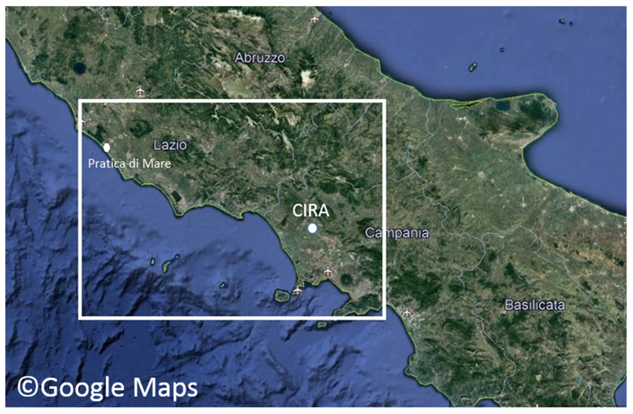
21]. A convective-scale model configuration characterized by a horizontal resolution of about 1 km has been developed at CIRA and is running daily over the area (12.22°–14.55° E; 40.63°–41.88° N) (
Figure 1) located in southern Italy. The computational domain has 260 × 138 points, while the number of vertical levels is set equal to 60. The time step is set equal to 10 s. Initial and boundary conditions are provided by the ECMWF IFS global model [
22] at spatial resolution of 0.075°.
The capabilities of the COSMO model over this domain in simulating the main atmospheric variables have been already tested against data provided by the CIRA weather instrumentation and other data and the results were presented in [
23]. In particular, wind values were validated against data provided by the wind profiler installed at CIRA (owned by ARPAC – Environmental Protection Agency of Campania region) revealing good model performances, suggesting a great potential of the model to support forecasts for drone flights.
Figure 1.
The computational domain considered, including part of Campania and Lazio regions. The CIRA location is specified.
Figure 1.
The computational domain considered, including part of Campania and Lazio regions. The CIRA location is specified.
For the purposes of the present work, COSMO output data over a 10 x10 subgrid have been extracted for the MPM application. This subgrid is centred over the target point located at CIRA facilities (
14.160 E; 41.120N) (shown in
Figure 1). The original coordinate values in degrees have been converted in meters, assuming the bottom-left point of the subgrid as origin (0,0).
4.2. Observational Data
Model evaluation has been conducted using 10-metres wind values provided by two weather stations MAWS301 installed at CIRA. They are produced by Vaisala, powered by photovoltaic panels and equipped with a 12 V 27 Ah buffer battery. Specifically, Weather Station 1 is equipped with various sensors for measuring several atmospheric variables while Weather Station 2 is only equipped with an anemometer for measuring the wind at 10 meters (direction and intensity). For each of the two weather stations, data reception occurs via a data logger positioned at the base of the pole, which communicates via radio-modem with an antenna positioned on the roof of the CIRA main building, in line of sight with the two transmitting antennas. These communications take place in UHF and the frequency used is set at 395 MHz. Furthermore, a dedicated software automatically creates two text files per day (one for each station) in which all the measurements taken over the course of 24 hours are saved, with a time resolution of 1 m.
5. Description of the Methodology
The coupling of MPM with the LAM COSMO has been realized in such a way that the MPM reads the hourly NWP output at high resolution over the considered subgrid, generates particles at each grid points and provides wind values every minute in the generical point considered for the investigation.
The tool works through the following steps:
the daily output NWP files related to a subgrid are read. This subgrid is made up of n x n points (in the present study, as already stated, n has been set equal to 10) centered over the location object of investigation and contains 24 hourly values of 10-metres wind velocity (horizontal u and v components).
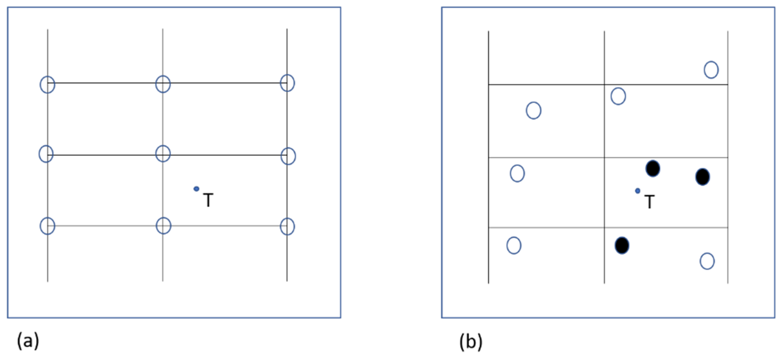
for each of the 24 hours, a family of N particles is generated, which are initially located in the grid points (
Figure 2a) and are characterized by a velocity equal to the wind velocity in the corresponding points. The age of this family (α) is initially equal to zero, but at each successive hour its age is increased by 1 unit.
for each of the 60 minutes of the current hour, the updated position of the particles is calculated, considering their own velocity components ui, vi (with i=1 … N):
in which the
ΔP factors are calculated as:
meaning that the particles move according with a random track horizontal motion, characterized by a small bias (σ), conveniently controlled by the
k2 factor (particle random walk factor), which was originally set equal to 10 in ref. [
7], but modified for other applications (e.g. it was set equal to 8 in ref. [
9]). The time step Δt is equal to 1 m.
Then, the three particles closest to the target point are individuated by means of an exhaustive research and the provisional velocity in the target point is calculated as weighted mean of the velocity values of these three particles (
Figure 2b). The weight to be assigned to each particle is calculated as function of the distance of the target point from the particle itself.
where α is a number that represents the age of the particle and
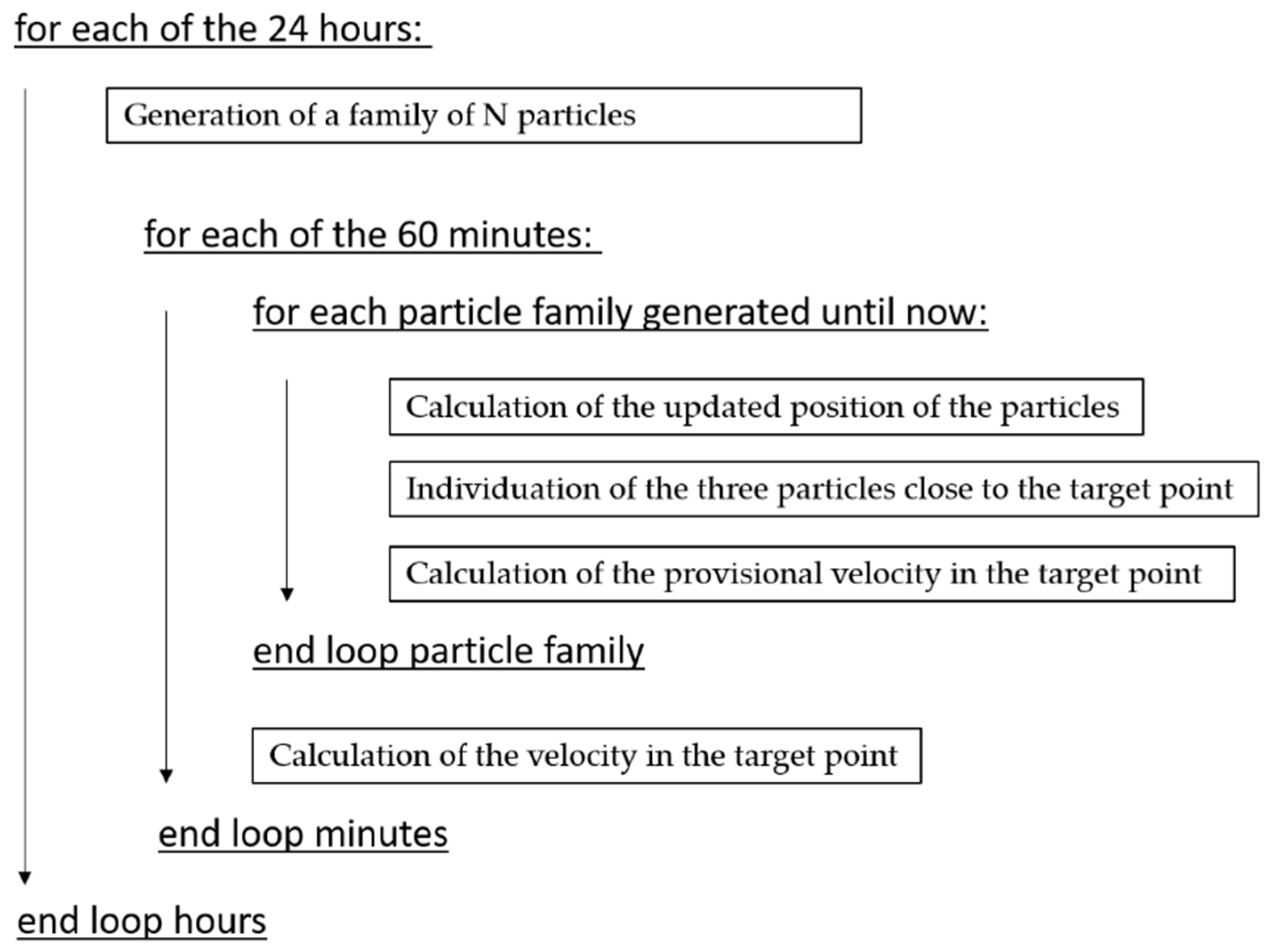
Cα is a control parameter (aging parameter) chosen by the user. It could be set equal to 30, according with the indications of the authors of the method. The algorithm is summarized in
Figure 3.
Figure 2.
(a) An example of grid points and initial location of the particles. (b) Location of the particles after some steps and individuation of the three particles (black) closest to the target point T.
Figure 2.
(a) An example of grid points and initial location of the particles. (b) Location of the particles after some steps and individuation of the three particles (black) closest to the target point T.
Figure 3.
Graphical representation of the algorithm used.
Figure 3.
Graphical representation of the algorithm used.
6. Results
The coupled NWP-MPM system has been tested for each day of the period from 1 to 30 June 2020 considering three different MPM configurations. Each configuration is characterized by specific values of the control factors defined in the previous sections, as summarized in
Table 1. These values have been chosen according with experiments performed and considering recommendations provided in specific literature works. As described later, the first configuration (Config 1) provided the best results and was selected for a more detailed analysis.
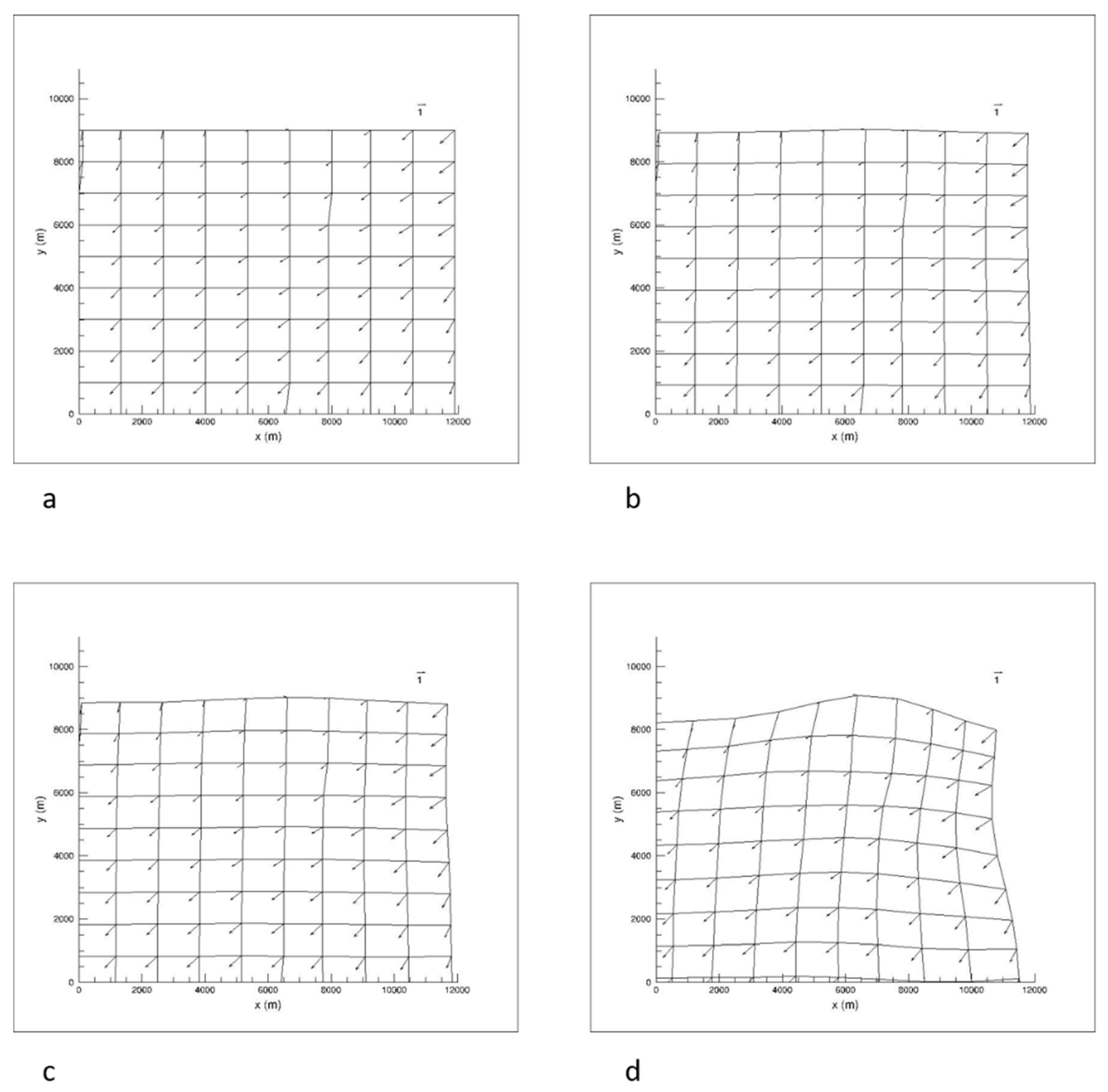
Figure 4 shows the position of the first family of particles for 1 June 2020 respectively at (a) the beginning of the simulation at 1:00 am (which is assumed as t = 0) and after (b) 1 m, (c) 2 m and (d) 10 m. The velocity vectors that characterize each particle are shown too. The 10 x 10 subgrid extracted from COSMO is visible in
Figure 4a: in fact, as already described, at the beginning of the simulation the position of the particles coincides with those of the grid points.
Figure 5 shows the wind field reconstruction performed by the MPM after 1 m in the neighborhood of the target point (5560 m, 4670 m). The wind vectors reconstructed in sample points at a distance of 100 m one another in the two directions are represented by red arrows, while the original wind vectors provided by COSMO are represented by black arrows.
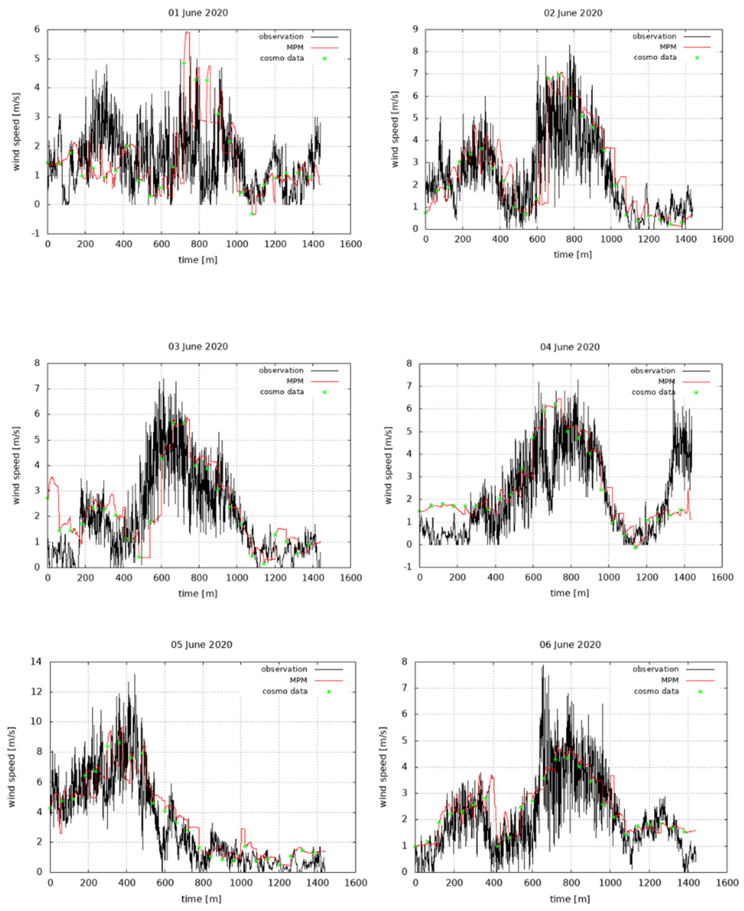
Figure 6 shows the time series of wind speed for the days from 1 to 6 June 2020, provided by MPM and by the weather station at frequency of 1 m. The original COSMO data (for the grid point closest to the target one) are also shown (identified by green asterisks), which are available every hour. These plots reveal a good behavior of the MPM in reproducing the general trend of wind speed over the whole days considered, in particular the wind increase that is observed almost every day between 600 and 800 m (i.e. between 11 a.m. and 1 p.m.) is well captured. Non-negligible discrepancies are however observed in some days, in particular in the last hours of each simulation, along with some overestimations in the central part of the day, in particular on 1 June2020. It is worth noting that most of inaccuracies are inherited by the COSMO model output, however MPM is able to overperform the NWP model, as discussed later. The time series have been processed by using an FFT aimed to produce a power spectrum of wind at regularly spaced bins, to measure the amounts of variability occurring in different frequency bands.
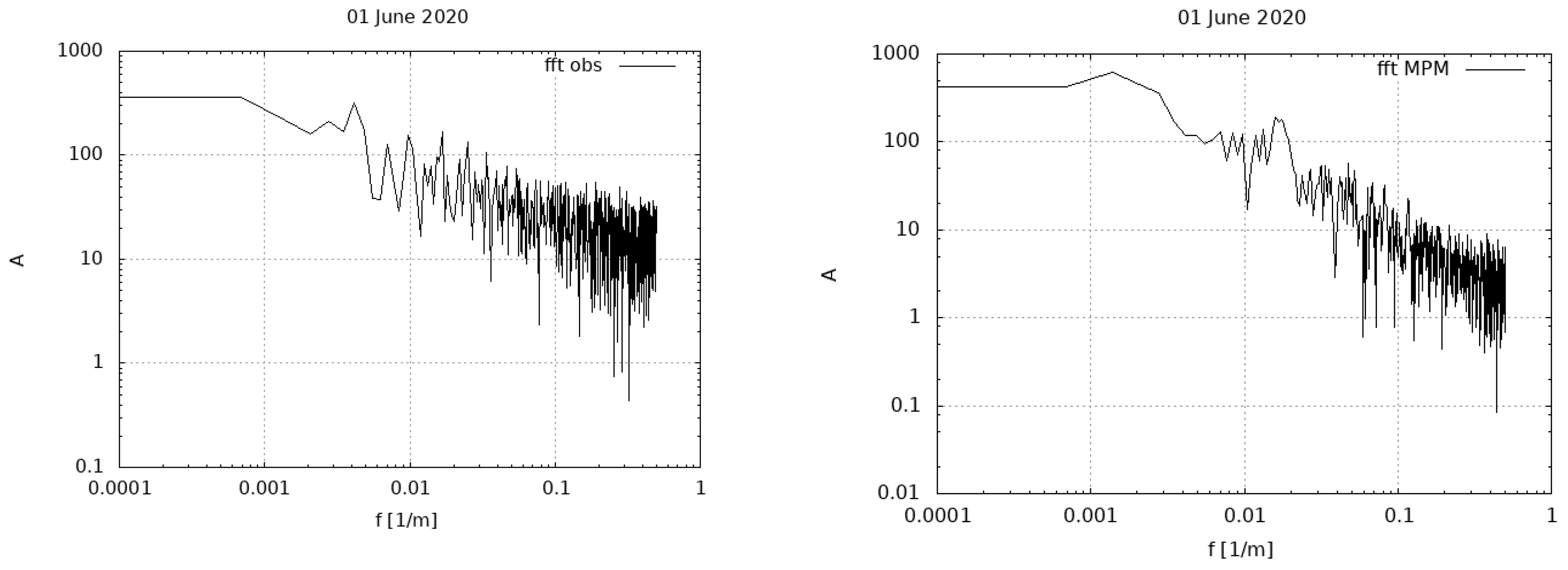
Figure 7 shows the mean power spectra (log-log representation) related to the time series of 1 June 2020, respectively related to observational data (left) and MPM data (right). It can be observed that the two spectra appear similar and that the main observed frequency (0.0027, corresponding to a period of 6 hours) is well captured by the model.
In order to quantify model performances, standard indices for performance evaluation have been calculated: mean bias (BIAS) and root-mean-square error (RMSE), defined as:
where
Si and
Oi are, respectively, the simulated and observed values at the
i-th time step.
N is the number of time steps considered (1440 for each day).
Table 2 shows the numerical values of these indicators related to the wind speed for COSMO and MPM (three configurations) with respect to observations, obtained considering the whole period (1-30 June 2020). Specifically, BIAS and RMSE speed are obtained considering daily values first and then averaging them over the thirty days considered. Max BIAS speed is the maximum values among the thirty daily values. The analysis of
Table 2 reveals that the best performances of MPM are obtained with Config 1 and that MPM is able to overperform the NWP COSMO on average, even if in some days the MPM is characterized by larger biases.
Table 3 shows the numerical values of the same indicators related to the wind direction (°) for COSMO and MPM (three configurations) with respect to observations, over the same period. It can be seen that even if the model overperforms the COSMO output, direction accuracy in some days is rather scarce, as also observed in [
14], especially at smaller wind speeds.
Table 2.
Numerical values of BIAS and RMSE of wind speed (m/s) for COSMO and MPM for three different configurations with respect to observations, obtained as average values over the period 1-30 June 2020.
Table 2.
Numerical values of BIAS and RMSE of wind speed (m/s) for COSMO and MPM for three different configurations with respect to observations, obtained as average values over the period 1-30 June 2020.
| Model |
BIAS Speed |
Max BIAS Speed |
RMSE Speed |
| COSMO |
0.10 |
0.24 |
0.46 |
| MPM 1 |
0.03 |
0.84 |
0.37 |
| MPM 2 |
0.04 |
0.88 |
0.39 |
| MPM 3 |
0.07 |
0.92 |
0.52 |
Table 3.
Numerical values of BIAS and RMSE of wind direction (°) for COSMO and MPM for three different configurations with respect to observations, obtained as average values over the period 1-30 June 2020.
Table 3.
Numerical values of BIAS and RMSE of wind direction (°) for COSMO and MPM for three different configurations with respect to observations, obtained as average values over the period 1-30 June 2020.
| Model |
BIAS Direction |
Max BIAS Direction |
RMS Direction |
| COSMO |
14 |
81 |
26 |
| MPM 1 |
12 |
72 |
24 |
| MPM 2 |
16 |
68 |
32 |
| MPM 3 |
19 |
88 |
36 |
7. Conclusions
In the present work, a methodology for wind field reconstruction based on the Meteo Particle Model from Numerical Weather Prediction data was presented. The problem of wind forecasting is particularly felt for aeronautical applications; in fact, several studies (e.g. [
24]) have examined the effect of errors in wind forecasting on Continuous Descent Operations, finding that an accurate knowledge of wind conditions is important since about 2/3 of the errors is due to an incorrect wind forecast. Moreover, meteorological conditions in urban environments require detailed analysis because of the influence that the characteristics of the urban fabric can have on local meteorological conditions. The impact can be more or less significant, depending on the field of applications. Beyond applications to drones, the present approach for low-altitude wind reconstruction can also be applied to other cases, e.g. Ship Helicopter Operational Limitation analysis [
25], crane safety in the construction industry [
26], and as a further input to national meteorological services.
The coupling of MPM with the LAM COSMO has been implemented in such a way that the MPM reads the NWP output at high resolution over a selected and provides wind values in the generical point considered for the investigation. The numerical results obtained revealed a good behavior of the method in reproducing the general trend of wind speed, as confirmed also by the power spectra analysis. The MPM is able to step over the intrinsic limitations of the NWP model in terms of spatial and temporal resolution even if, as expected, the MPM inherits the bias that inevitably affects the COSMO output. For this reason, in the opinion of the author, a step forward will be represented by the application of a bias correction technique [
27] to the NWP output, performed considering a validation period in which observed and modelled time series are available and overlapped. In fact, the NWP post-processing has become a standard practice, for example by using the Model Output Statistics (MOS) that model the bias as a function of input variables or the Kalman filter, a technique that estimates the true state of a dynamical system from noisy measurement data [
28].
Although not within the scope of the present project, it would also be useful to open a future perspective where the training of the MPM methodology can start to consider the structures and obstacles present in specific urban environments. Given that the training of particles still requires a specific task for the single urban area, it could be useful to underline the importance of installing specific sensors capable of measuring wind variations in the vicinity of obstacles or structures to configure particles more appropriately.
Funding
This research was carried out in the frame of the CIRA internal project PRORA 662 SESAAM EDUS, funded by the DM 662/2020 of the Italian Ministry of Education.
Data Availability Statement
Data stored at CIRA supercomputing center and available on request.
Acknowledgments
Vittorio Di Vito (CIRA) and Giulia Torrano (CIRA) are gratefully acknowledged for the effective management of the EDUS project.
Conflicts of Interest
The author declares no conflict of interest.
References
- SESAR JU, European ATM Master Plan: Roadmap for the safe integration of drones into all classes of airspace, Tech. Rep., Mar. 2017; available at https://www.sesarju.eu/node/2993 (accessed 06/10/2023).
- Kalman RE, A New Approach to Linear Filtering and Prediction Problems, Transaction of the ASME – Journal of Basic Engineering, 82, Series D, 1960, 35–45. [CrossRef]
- Mondoloni S, A Multiple-Scale Model of Wind-Prediction Uncertainty and Application to Trajectory Prediction, Proc. 6th AIAA Aviation Technology, Integration, and Operations Conference (ATIO), Wichita, Kansas, September 25–27, No. AIAA 2006-7807, 1–14, 2006.
- De Jong PMA, Van der Laan JJ, In ‘t Veld AC, Van Paassen MM, Mulder M, Wind-Profile Estimation Using Airborne Sensors, Journal of Aircraft, 2014, 51, 6, 1852–1863.
- de Leege A, Van Paassen M, Mulder M, Using automatic dependent surveillance-broadcast for meteorological monitoring. Journal of Aircraft, 2012, 50(1), 249-261. [CrossRef]
- Kiessling J, Ström E, Tempone R, Wind field reconstruction with adaptive random Fourier features, Proc. R. Soc. A 2021, 477, 20210236. [CrossRef]
- Sun J, Vû H., Ellerbroek J, Hoekstra JM, Weather field reconstruction using aircraft surveillance data and a novel meteo-particle model. PloS one, 2018, 13(10). [CrossRef]
- Sunil E, Koerse R, Brinkman T, Sun J, METSIS: Hyperlocal Wind Nowcasting for U-space, 11th SESAR Innovation days, 2021, https://www.sesarju.eu/sites/default/files/documents/sid/2021/papers/SIDs_2021_paper_88.pdf (accessed 08/08/2023).
- Zhu J, Wang H, Li J, Xu Z, Research and Optimization of Meteo-Particle Model for Wind Retrieval, Atmosphere 2021, 12, 1114. [CrossRef]
- Bucchignani E, Methodologies for wind field reconstruction in the U-SPACE: a review, Atmosphere, 2023 14, 1684. [CrossRef]
- Rillo V, Zollo AL, Mercogliano P, MATISSE: an ArcGIS tool for monitoring and nowcasting meteorological hazards, Advances in Science and Research, 2015, 12(1), 163–169. [CrossRef]
- Steppeler J, Doms G, Bitzer HW, Gassmann A, Damrath U, Gregoric G, Meso-gamma scale forecasts using the nonhydrostatic model LM. Theor. Appl. Clim. 2003, 82, 75–96. [CrossRef]
- Zängl G, Reinert D, Rípodas P, Baldauf M, The ICON (ICOsahedral Non-hydrostatic) modelling framework of DWD and MPI-M: Description of the non-hydrostatic dynamical core. Q. J. R. Meteorol. Soc. 2015, 141, 563–579. [CrossRef]
- Sunil E, Koerse R, Brinkman T, Sun J, METSIS: Hyperlocal Wind Nowcasting for U-space, 11th SESAR Innovation Days. 2021. Available online: https://www.sesarju.eu/sites/default/files/documents/sid/2021/papers/SIDs_2021_paper_88.pdf (accessed on 8 August 2023).
- Sun J, Vu H, Ellerbroek J, Hoekstra J, Ground-Based Wind Field Construction from Mode-S and ADS-B Data with a Novel Gas Particle Model, 7th SESAR Innovation Days. 2017. Available online: https://www.sesarju.eu/sites/default/files/documents/sid/2017/SIDs_2017_paper_16.pdf (accessed on 8 August 2023).
- de Leege, A.M.P, van Paassen M.M, Mulder M, Using automatic dependent surveillance-broadcast for meteorological monitoring. J. Aircr. 2012, 50, 249–261. [CrossRef]
- de Haan, S. High-resolution wind and temperature observations from aircraft tracked by Mode-S air traffic control radar. J. Geophys. Res. Atmos. 2011, 116, D10. [CrossRef]
- Kanamitsu M, Description of the nmc global data assimilation and forecast system. Weather. Forecast. 1989, 4, 335–342. [CrossRef]
- Hersbach H, Bell B, Berrisford E, Hirahara S, Horányi A, Muñoz-Sabater J, Nicolas J, Peubey C, Radu R, Schepers D, et al. The ERA5 global reanalysis. Quart. J. Royal Met. Soc. 2020, 146, 1999–2049. [CrossRef]
- Mazzarella V, Milelli M, Lagasio M, Federico S, Torcasio R.C, Biondi R, Realini E, Llasat M.C, Rigo T, Esbrí L, et al. Is an NWP-Based Nowcasting System Suitable for Aviation Operations?. Remote. Sens. 2022, 14, 4440. [CrossRef]
- Doms G, A Description of the Nonhydrostatic Regional COSMO Model, Part I: Dynamics and Numerics; Technical Report; Deutscher Wetterdienst: Offenbach, Germany, 2002.
- Hortal M. The development and testing of a new two-time-level semi-Lagrangian scheme (SETTLS) in the ECMWF forecast model. Q. J. R. Meteorol. Soc. 2002, 128, 1671–1687.
- Bucchignani E, Mercogliano P, Performance Evaluation of High-Resolution Simulations with COSMO over South Italy, Atmosphere, 2021, 12, 45. [CrossRef]
- Klooster J. Wichman K, Bleeker O, 4D Trajectory and Time-of-Arrival Control to Enable Continuous Descent Arrivals. In Proceedings of the AIAA Guidance, Navigation and Control Conference and Exhibit, Guidance, Navigation, and Control and Co-located Conferences, Honolulu, Hawaii, 19 August 2002.
- Hodge SJ, Forrest J, Padfield GD, Owen I, Simulating the environment at the helicopter-ship dynamic interface: Research, development and application, Aeronautical Journal -New Series, 2015, 116(1185),1155. [CrossRef]
- Neitzel R, Seixas N, Ren, KK, A Review of Crane Safety in the Construction Industry, Applied Occupational and Enviromental Hygiene, 2002, 16(12):1106-17. [CrossRef]
- Teutschbein C, Seibert J, Bias correction of regional climate model simulations for hydrological climate-change impact studies: Review and evaluation of different methods, Journal of Hydrology, 456–457, 12–29. 2012. [CrossRef]
- Yang D, On post-processing day-ahead NWP forecasts using Kalman filtering, Solar Energy, 2019, 182:179-181. [CrossRef]
|
Disclaimer/Publisher’s Note: The statements, opinions and data contained in all publications are solely those of the individual author(s) and contributor(s) and not of MDPI and/or the editor(s). MDPI and/or the editor(s) disclaim responsibility for any injury to people or property resulting from any ideas, methods, instructions or products referred to in the content. |
© 2023 by the authors. Licensee MDPI, Basel, Switzerland. This article is an open access article distributed under the terms and conditions of the Creative Commons Attribution (CC BY) license (http://creativecommons.org/licenses/by/4.0/).
