
You are currently viewing a beta version of our website. If you spot anything unusual, kindly let us know.
Preprint
Article
Simulation-Based Education Tool for Thermostatically Controlled Loads Understand
Altmetrics
Downloads
87
Views
44
Comments
0
A peer-reviewed article of this preprint also exists.


This version is not peer-reviewed
Abstract
Thermostatically controlled loads have great potential to make a significant contribution to improving energy efficiency in the building sector, which is responsible for 40% of greenhouse gas emissions in the EU. This, in addition to the environmental damage, represents a huge expense in the electricity bill. Therefore, it is very important to train engineers on how to design energy management systems for TCLs. With this goal in mind, it would be very useful to have a simulation-based educational tool (SBET) to understand thermostatically controlled loads, their characteristics and possibilities in energy efficiency. In addition, it would be very useful if this tool could be introduced in engineering curricula to help students to be better trained and enter the labor market with more opportunities. Based on the shortcomings detected, this work develops a SBET specifically designed to teach about TCLs (SBET-TCLs), both about their intrinsic characteristics and their better management. To verify the developed SBET-TCL, it has been tested in a real scenario: A survey was carried out among the students of the subject 'Alternative Energy Sources' of the degrees of Industrial Engineering. The results show that the use of SBET-TCL has very positive effects on the learning process.
Keywords:
Subject: Engineering - Electrical and Electronic Engineering
1. Introduction
The current geopolitical situation and the enormous problems of climate change to which the world is subjected, require solutions in the short term to alleviate energy costs on the one hand and, on the other, to begin a gradual process of decarbonization of the planet that will allow at least a glimpse of a future of guaranteed sustainability. Focusing on the electricity sector, it is necessary to decisively address two major problems: reduction of electricity costs (at the end of the chain the bill paid by the user) and increase in the penetration of renewable energies. In this complex scenario, thermostatically controlled loads (TCLs), mainly electric space heating/cooling, refrigerators, freezers, and electric water heaters, have great potential to minimize electricity bills and maximize the penetration of renewables in the electricity system [1]. In fact, heating and cooling loads represent around half of the total energy consumption of EU countries [2]. However, due to the thermal characteristics of the TCLs, by applying appropriate control strategies it is possible to increase or reduce their power, or even make the temporary displacement of TCLs connection without loss of thermal comfort for the user, simply by taking into account the intrinsic thermal storage capacity of the buildings [3]. Thus, to reduce global energy consumption and CO2 emissions in buildings, TCL modeling and control is an excellent resource [4] since it brings a numerous benefits when energy demand is high [5] or energy cost wants to be minimized [6].
Based on the above, despite being a novel field of research, it is necessary to incorporate the management of TCLs in the curricula of students, with emphasis on higher education and engineering careers.
The constant evolution of society and technology implies the need for constant revision of engineering curricula [7]. In engineering education, theoretical concepts are often complex and difficult to bring to real life, thus, practical activities play a very important role in learning. However, open-air activities [8] or real laboratory experiments [9] require expensive equipment, are time-consuming and can involve a certain amount of danger. In particular, teaching TCL control in real laboratories requires complex and expensive equipment, as well as environmental conditions (those corresponding to a real inhabited building: home appliances, insulation, room temperature, etc.) and availability of time of use that are very difficult to achieve.
To overcome the above mentioned drawbacks, simulation-based educational tools (SBETs) can be an excellent choice to complement and enhance the quality of learning about TCLs.
In general, SBETs have been playing an important role in the teaching-learning process for years [10]. Indeed, SBETs have been shown to help both teachers by optimizing educational content, and students by improving comprehension and increasing interest and creativity [11].
There are studies that analyze the learning progress student of groups of students who use SBETs versus those who do not [12]. Results show that groups of students using SBETs have a better learning rate. In fact, according to [13], SBETs allow students to retain up to 90% of educational content, as opposed to reading (10%) or listening (20%).
On the road to place the student at the center of the learning process, novel approaches to learning in science education have emerged in recent years. Examples include collaborative [14], problem-based [15], project-based [16], and competency-based learning [17], along with the flipped classroom [18] and gamification techniques [19], among others. Practices carried out in classroom through these methodologies can be enhanced with different technological applications, resulting in a pedagogical approach known as blended learning [20]. Thus, SBETs are a suitable resource to overcome the challenges and difficulties of the learning process [18,21].
The current digital transformation process has also promoted these new educational approaches. However, until the COVID-19 pandemic, its impact had not been as pronounced as it is now [22,23]. In fact, it is after the COVID-19 pandemic that a European Union (EU) policy initiative known as Digital Education Action Plan (2021-2027) appears, whose aim is to support the adaptation of member states’ education and training systems to the digital age [24].
Perhaps, at the forefront of this transition towards teaching with the student as the protagonist of his own learning process, towards a more digital education are the universities [25]. In this framework, students’ interest and motivation increase, and the development of their skills is facilitated.
SBETs can be self-developed [26,27,28] or commercial [29,30,31,32], and involve virtually all engineering degrees. In this way, there are applications in electrical [33], electronic [34,35], communications [36], control [37,38], computer science [39], thermal energy [40] or mechanic [41], among others.
Focusing on the field of TCLs, there are some simulation-based tools in the literature that can manage them [42,43,44,45,46], but not specifically, but as part of a network, usually an electrical network. Moreover, although these tools can be used in educational environments, they are not developed for that purpose, so, among other things, they lack the necessary utilities to deepen the intrinsic knowledge of TCLs. Therefore, and in this sense, they cannot be considered SBETs. Thus, GridLAB-D™ [42] was developed by the U.S. Department of Energy (DOE) and envisions the management of TCLs as just another load in an electrical distribution system. On the other hand, the Object-oriented, Controllable, High-resolution Residential Energy (OCHRE) tool [43] does not deal in a specific way with TCLs but can include them in its simulations as thermal loads. As for OpenDSS [44], it is an electrical power distribution system simulator that can handle TCLs as loads with specific hourly operation, but not as a control system to optimize them. Finally, [45,46] are designed for the microgrids simulation. Thus, RAPSim (Renewable Alternative Powersystems Simulation), [45], is a free and open source microgrid simulation framework whose main objective is to foster the understanding of power flows in smart microgrids with renewable sources. Again, TCLs are just another load. With regard to [46], HOMER Pro® microgrid software by HOMER Energy is a high-level simulation payment framework. Its capabilities are enormous, but it does not delve, or even go into, the nature of TCLs as they are of interest in an academic setting.
After analyzing the state of the art of the availability of SBETs in the literature for the in-depth study of TCLs, it was concluded that there were no tools suitable for academic environments. Consequently, this was the motivation for the work presented in this article: a specific SBET for TCLs (SBET-TCLs).
This paper presents a SBET-TCLs that allows to study in depth the dynamic behavior, energy consumption and best management of the TCLs in buildings (in the following and throughout the paper, building, house or dwelling may be used interchangeably) applications: electric space heating/cooling, refrigerators, freezers, and electric water heaters. Due to the experience in previous developments, the simulation tool was implemented using Easy Java/JavaScript Simulations (EJS) [47], an open source tool written in Java, mainly dedicated to teaching and learning purposes.
The main objective of this research is to improve, through the development and use of a new SBET, the learning of TCLs, facilitating their understanding and practical applicability. Then, following the line of previous education works of the authors and aiming to measure the suitability of the proposed SBET, a survey has been carried out among the students of the subject ‘Alternative Energy Sources’ of the degree courses in Electrical Engineering, Industrial Electronic Engineering, Mechanical Engineering and Industrial Chemical Engineering. Results show that the use of the developed SBET improves the learning process on TCLs in these degrees.
Based on everything discussed in this section, this paper is novel for the following reasons:
(1) Prior to the proposed SBET, there were no tools suitable for academic environments specifically focused on the TCLs teaching/learning process.
(2) The proposed SBET delves deeper into the intrinsic behavior of TCLs, i.e., it allows them to be studied at the lowest level.
(3) The proposed SBET allows modeling TCLs as state space models, which captures their dynamics.
(4) The proposed SBET works with parameterized models that can be easily modified by the student according to the application under study.
(5) The proposed SBET is a very intuitive and easy framework, which is essential in an educational environment, otherwise the student will be demotivated by the workload.
(6) The proposed SBET has been incorporated into curricula and tested in real engineering degree scenarios.
(7) To the authors’ knowledge, there is no TCL model in the literature that is more intuitive, simpler, and easier to calculate and interpret than the one presented in this article.
The remainder of this paper is organized as follows. Firstly, the article presents the theoretical framework and the methods to know some necessary parameters in the developed models in Section 2.1 and Section 2.2, respectively. Then, the educational framework is described in Section 2.3. A description of the developed simulation-based educational tool is given in Section 3. Next, the results about the technical performance of the developed simulation-based educational tool and their evaluation as an educational resource are reported in Section 4.1 and 4.2, respectively. Results obtained are discussed in Section 5. Finally, some conclusions are drawn in Section 6.
2. Materials and Methods
The materials and methods used in the SBET development can be divided into two distinct parts. The first one refers to the technical aspects of the tool, that is, what is its scientific basis thermodynamically speaking. The second refers to the educational aspects of the tool, that is, its evaluation as an educational resource.
2.1. Theoretical framework of the developed simulation-based education tool
As already explained, the usual TCLs in a building are considered in the study: electric space heating/cooling, refrigerators, freezers, and electric water heaters. Each TCL is modeled following an approach known as grey-box model [48], which are dynamic thermal models (state-space models) identified from experimental measurements [49]. The main concept of the grey-box models is to group and represent the different components of the TCLs by means of thermal resistances (R), representing the difficulty in the heat transfer (i.e. the degree of tightness of the thermal enclosures), and thermal capacities (C), which represents the capacity to store energy in the form of heat. This is analogous to the way an electrical circuit hinders the passage of electric current through resistors and stores electrical energy through capacitors. As a simple example, consider a building in which air infiltration losses through the windows are not taken into account, nor the temperature difference between the ambient temperature and that of the walls. In this case, any room with exterior walls has two thermal nodes (interior and exterior wall surface) with their respective thermal capacities connected by a thermal resistance representing the rate of convective and radiative heat exchange between them through the wall.
This type of RC model must be identified, i.e., applied to the example of the building, the different values of R and C in the different parts of the building due to the different TCLs have to be calculated or measured [50]. The value of C depends on the node’s ability to store energy in the form of heat; think, for example, of the outer surface of a wall that absorbs energy depending on the solar radiation, its color and physical composition. Regarding R, the higher the thermal insulation of the wall, the higher its value because it opposes the heat transfer between the nodes representing the internal and external surfaces.
Models are formulated using the discrete time state-space representation. In the linear case as in (1) - (2); developed from [51].
The state equation (1) is the result of the thermodynamic analysis of the TCL, which leads to a system of as many first-order differential equations as there are energy storage elements in the model (thermal capacities). As for the output equation (2), it can be observed that it has not dynamic and is decided by the designer, usually with an output vector with as many coordinates as variables of interest that can be measured.
In detail, is the sampling, is the state vector, the order of the model (the number of first-order differential equations), is the input vector, where p is the number of inputs, is the state matrix, the input matrix, and the vector of m model parameters. Note that the parameter vector depends on discrete time because the TCL conditions can vary with time; think for example of an open/closed window or open/closed refrigerator door (please, see Appendix).
As for the output equation (2), is the output vector, where q is the number of outputs, and is the output matrix.
Next, based on the physical principles established so far, the state space models for each TCL included in the proposed SBET will be developed.
2.1.1. Electric space heating/cooling
The development of this model is based on [49]. The state, input and output vectors of the model are written, respectively, in (3).
Where the state vector is make up by the temperature at each thermal node due to the corresponding thermal capacity, three in this case: the interior building wall temperature , the exterior building wall temperature , and the indoor air temperature or interior ambient temperature due, respectively, to the thermal capacities , and . This model considers the interior ambient temperature as a separate temperature node of the interior building wall temperature node , which adds accuracy to the model because, in general, the ambient temperature and the wall temperature are different. Regarding the input vector , it is make up by the variables that force the temperature changes of the building. These are the outside building air temperature or exterior ambient temperature (this model considers the exterior ambient temperature different from the exterior building wall temperature since in general both are different; again, this adds accuracy to the model) that influences by the wall thermal conduction and the opening of doors and/or windows, electrical power consumed by the building for heating/cooling and irradiance , or energy per unit area of global solar radiation incident on a horizontal surface of the building. It is calculated according to the position and orientation of the building, as well as its geographical location (latitude and longitude) [52]. Finally, the output vector coincides with the state vector (this facilitates the use of the state vector for controller design because all its coordinates can be measured [53]) and represents the evolution of the temperatures of each of the thermal nodes. The model matrices are (4) - (6).
Where , , and are, respectively, the thermal resistances between nodes and , and , and , and . Thus, following (1) - (2), , , , , , ; values of these model parameters are listed in Table A1 of Appendix A. Finally, numerical values ( and ) can be observed in matrix B, whose meanings are coefficients to fit the model.
In what follows, the meaning of the subscripts of the variables is the same for the rest of models. Of course, taking into account in each case the physical environment of each TCL.
2.1.2. Refrigerator
The development of this model is based on [54]. The state, input and output vectors of the model are written, respectively, in (7).
Where the state vector is make up by the interior refrigerator temperature and the exterior temperature of the refrigerator housing due, respectively, to the thermal capacities and . In this case, due to the interior volume of the refrigerator housing (considerably lesser than that of a room in a building) and its degree of thermal insulation (considerable larger than that of a room in a building) both the interior ambient temperature and the temperature of its interior walls are considered to be the same,. As for the input vector , it is make up by the variables that force the temperature changes of the refrigerator: air temperature around the refrigerator, i.e., the interior ambient temperature of the building (this model considers the exterior ambient temperature around the refrigerator housing different from the exterior temperature of the cooler housing since in general, both are different; this adds accuracy to the model) that influences by the refrigerator housing thermal conduction and the opening of its door, and the electrical power consumed for cooling . Finally, the output vector coincides with the state vector and represents the evolution of the temperatures of each of the thermal nodes. The model matrices are (8) - (10).
Where , , and are, respectively, the thermal resistances between nodes and , and , and . Thus, following (1) - (2), , , , ; values of these model parameters are listed in Table A2 of Appendix A.
2.1.3. Freezer
Following [55], the model of the freezer is analogous to that of the refrigerator, i.e. (7) – (10). Now power consumed for cooling is . Model parameters values are listed in Table A3 of Appendix A.
2.1.4. Electric water heater
The development of this model is based on [56]. The state, input and output vectors of the model are written, respectively, in (11).
Where the state vector is make up by the interior water temperature of the heater and the exterior temperature of the water heater housing due, respectively, to the thermal capacities and . As for the input vector , it is make up of the variables that force the temperature changes of the water in the heater: temperature of cold water supplied to the heater (when the water heater is receiving water from outside to compensate for the water it is supplying) and the electrical power consumed for heating . Faced with these input coordinates with a great influence on the changes in water temperature in the heater, thermal conduction of the heater housing is not taken into account (the water heater will normally be inside a cabinet and the heat exchange with the outside can be considered negligible compared to the daily inflow of cold water). Again, the output vector coincides with the state vector and represents the evolution of the temperatures of each of the thermal nodes.
Changing the corresponding subscripts and values, matrix A is the same as in (8), matrix B is the same as in (9), and matrix C is the same as in (10). Model parameters values are listed in Table A4 of Appendix A.
2.2. Temperature and irradiance measurement
As can be seen in the models of the Subsection 2.1, to calculate the electrical power consumed by the TCLs
it is necessary to have continuously available interior and exterior ambient temperatures to the building, interior and exterior wall temperatures as well as the irradiance to which the building is exposed. In addition, for the refrigerator and freezer, it is necessary to know the internal and external temperatures of their housings. Finally, as far as the electric water heater is concerned, it is necessary to know the temperature of the water inside it and the inlet temperature coming from the supply to the building.
In general, obtaining temperature values is very simple, since it is enough to have thermometers for this purpose (many household appliances supply them directly; [57] is a very accurate and inexpensive device for measuring surface temperatures as in [58]), and even the ambient air temperature outside the building can be obtained directly from the weather stations available in all cities (in the larges there are usually different measurement points, which logically allows it to choose the closest one). The same applies to the temperature of the water stored inside the water heater (provided by the device itself). There are even water heaters that provide information on the inlet water temperature from the exterior. In any case, water supply companies provide graphs of water supply temperatures. For example, in the city of Huelva (southwestern Spain), the monthly supply temperatures for 2021 are shown in Table 1 [59].
That said with respect to the ease of measuring temperatures, the same does not apply to irradiance. The device for measuring solar radiation on a flat surface (irradiance) is called a pyranometer. It is an expensive meter that, in addition, requires special care in positioning for reliable measurements. Therefore, it is not easy, much less usual, for every building to have one. For this reason, the developed SBET-TCL calculates the irradiance instead of measuring it, for which equation (12) is used, which has been adapted from [60].
Where:
is the received irradiance in between the initial time and the final time considered.
is the solar constant or total solar irradiance, i.e. the total amount of energy received as solar radiation per unit time and area measured outside the Earth’s atmosphere in a perpendicular plane to the sun’s rays. The measured and accepted value is .
is the correction factor of due to the eccentricity of the Earth’s orbit around the sun [61]. Specifically, , where is the number of days between 1 (January 1) and 365 (December 31).
is the latitude of the building under study.
is the solar declination resulting from the tilt of the Earth’s rotation axis. The value of solar declination varies continuously throughout the year, from a maximum of at the boreal summer (austral winter) solstice to a minimum of at the boreal winter (austral summer) solstice, where is the obliquity of the ecliptic. Solar declination is zero at the spring and autumnal equinoxes. .
is the solar angle, 0 at noon, negative in the mornings, and with a variation of 15° per hour from noon on. Then, between and varies between and , respectively. Finally, is the number of days between 1 (January 1) and 365 (December 31).
2.3. Educational framework of the developed simulation-based education tool
The study involved undergraduate engineering students of the subject ‘Alternative Energy Sources’. In this subject, students learn about the most commonly used renewable energy sources and energy demand management. Within this last topic, concepts and applications of TCLs are presented. Until the incorporation of the proposed SBET-TCLs, teachers were teaching the TCL framework in a theoretical way, and there was no measure of the students’ learning progress in this scope, other than theoretical assessment.
To measure the suitability as an educational resource of the proposed SBET-TCLs, students were asked to fill out a questionnaire with a set of questions on a 5-point Likert scale (1 = strongly disagree and 5 = strongly agree). The questionnaire was organized in different sections, focusing on the students’ level of knowledge of the subject, and on computer simulation-based learning, as well as on aspects of acceptance, design and usability of the simulation tool together with general considerations. Table 2 shows the survey questionnaire. To conduct this survey, a total of 48 students of the subject ‘Alternative Energy Sources’ (fourth-year elective) from the undergraduate degrees in Electrical Engineering (21% of students), Industrial Electronic Engineering (21%), Mechanical Engineering (29%), and Industrial Chemical Engineering (29%) were asked. The study was carried out in the second semester of the 2021-2022 academic year. The questions listed in Table 2 were asked to the students during laboratory sessions, when the teacher was already aware that they had understood the necessary theoretical concepts about the TCLs.
3. Developed simulation-based education tool
In the following, the developed SBET-TCLs will be explained, both its internal structure and its interface and capabilities.
Figure 1 shows the interface that the student can see when accessing the tool through a XHTML page. The interface is very simple, intuitive, and easy to use. The student must enter the data and parameters corresponding to the desired simulation. Specifically, in the first line: the corresponding date (day, month and year) and the start time (hour, minute and second). In the example in Figure 1, January 3, 2021, 10 seconds after midnight.
In the second line, the simulation data must be entered: simulation time in minutes, step simulation in seconds, hysteresis band percentage (it is a percentage of the set point temperatures, i.e., in a real situation it prevents the respective thermostats of the appliances from switching on and off continuously) and the city where the building is. In the example shown in Figure 1 and by the same order: 1,440 min (24 h), samples every 10 s, allowable percentage of 5% temperature variation from the set point temperature and, finally, the city of Huelva (southern Spain) for the location of the building.
The third line includes the set points for the temperatures (°C) of the different TCLs, i.e., the winter and summer comfort temperatures in the building, as well as the refrigerator, freezer and electric water heater. In the example shown in Figure 1 and by the same order: 24 °C (this means that with the chosen hysteresis band (5 %), and taking into account that it is a winter day, the interior temperature of the building can drop up to 22.8 without activating the electric space heating; of course, the same applies to all other set point temperatures listed below), 20 °C, 3 °C, -20 °C and 55 °C.
The fourth line allows to take into account the variation of the thermal resistances due to the opening of doors and/or windows (building), doors (refrigerator and freezer), and the contact of the incoming cold water with the internal hot water each time the electric water heater is used (outgoing hot water is replenished with incoming cold water). The meaning of the ratio (%) of openings/housing envelope, door/watertight housing and hot/cold water is as follows in each case: surface area of the open doors and/or windows in relation to the surface area of the envelope of the building, surface of the open door in relation to the refrigerator and freezer watertight housing and, finally, in the case of the electric water heater is the percentage of stored hot water consumed in each use. In the example shown in Figure 1 and by the same order: 10% (sum of the doors and/or windows) of the total envelope of the dwelling is open to the exterior, 20% (the surface of the refrigerator door is one-fifth of its total watertight enclosure), analogous to the freezer but now only 17% and, finally, 25 % means that for each shower, one-quarter of the total hot water stored in the electric water heater is used and, subsequently, replaced by cold water.
The user can decide on the fifth line at what times and for how long the doors and windows of the building, the refrigerator and freezer door will be open, as well as how the water heater will be used. Of course, as for the use of the appliances, the casuistry can be infinite, so the tool offers only some representative options. In fact, what is really intended is that the student learns to know how the different types of uses affect consumption so that he/she can apply responsible use. In the example shown in Figure 1 the sequence is 1-1-1-1.
Finally, the last line of the interface allows to introduce the power (W) of the appliances that represent the TCLs; in the case of Figure 1: air conditioner/heater (2,500 W), fridge (700 W), freezer (1,500 W) and water heater (2,500 W).
The developed SBET-TCL was implemented by Easy Java Simulations (EJS) [47], an open-source tool written in Java, mainly for teaching and learning purposes. During the last decade, EJS has been widely used in educational research in engineering, specifically in automatic control [62], robotics [63] and automation [64] among others. Moreover, after years of implementation and use of remote laboratories in higher engineering studies, the authors of this work have already achieved sufficient experience with this tool.
As for the structure of the developed SBET-TCL, it is shown in Figure 2 and will be explained below. First, the tool loads the data entered by the user through the interface of Figure 1. Then loads the models with their parameters (Subsection 2.1 and Appendix A, Table A1, Table A2, Table A3 and Table A4). To these, the temperature data are added. From here, the irradiance is calculated by (12). Now, once the models have been updated, the consumed power by each TCL can be calculated. In this sense, the algorithm takes into account the hysteresis band selected by the user, as well as the setpoint temperature of each TCL. If this is within the hysteresis band, the corresponding TCL does not consume power.
The algorithm runs in a loop until the end of the simulation time () chosen by the user in the interface (Figure 1). Note that temperatures should be updated at each sampling. The same is true for the model parameters, which will be updated depending on the user’s choice (Figure 1) of the sequence for openings/housing envelope, door/watertight housing and hot/cold water. For that, the algorithm loads the proper data (please see Appendix A, Table A1, Table A2, Table A3 and Table A4) of , and . When the algorithm goes out of the loop, the chosen simulation time has finished and the integration of the power over the simulation time delivers the energy consumed. As will be seen in the following section on results, the SBET-TCL provides a set of graphs and tables that allow a detailed analysis of consumption.
4. Results
In this work, the results are of two types, namely, those due to the technical performance of the developed SBET-TCL and those corresponding to the evaluation of the SBET as an educational resource.
4.1. Technical performance of the developed SBET-TCL
In order to obtain sufficient variability when displaying the results of the developed SBET-TCL, a winter day and a summer day have been chosen. For both, two different sequences (1-1-1-1 and 2-4-3-3) for openings/housing envelope, door/watertight housing, and hot/cold water (please, see Figure 1) have been taken into account. A total of four simulations were carried out.
The following figures (Figure 3, Figure 4, Figure 5, Figure 6, Figure 7, Figure 8, Figure 9, Figure 10, Figure 11, Figure 12, Figure 13, Figure 14 and Figure 15) show the behavior of the appliances regarding the interface set by the user and the environmental conditions of the dwelling. In the figures mentioned above, the indoor and outdoor temperatures are shown in blue and green, respectively, and the activation of the thermostat of each device and, consequently, the power consumption (always considering the nominal one), are in black.
Table 3 summarizes the energy consumption in each of the four scenarios considered.
Day: January 3, 2021. Sequence: 1-1-1-1. Its interface corresponds to that shown in Figure 1. Results are shown in Figure 3, Figure 4 and Figure 5.
Day: January 3, 2021. Sequence: 2-4-3-3. Its interface corresponds to that shown in Figure 6. Results are shown in Figure 7 and Figure 8. Of course, the daily irradiance is that of Figure 5.
4.2. Evaluation of the SBET-TCL as an educational resource
Students in the ‘Alternative Energy Sources’ course have evaluated SBET-TCL in the scenarios shown in Subsection 4.1. Among others designed by themselves, and with the objective of making them to realize the need of controlling TCLs, the test indicated in Table 4 has been proposed. As can be seen, it consists of three simulations. The first one is the base case with the parameters indicated in Figure 9, except hysteresis band. In the second one, all the parameter and kept constant except the building set point, which is increased from 24°C to 27°C. The parameters corresponding to the third simulation are the same as the corresponding to the second one, except the hysteresis band, which has been highly increase. The rest of initial parameters not included in Table 4 are the corresponding to Figure 9. The total consumption obtained in each case is presented in Table 4.
Now, once checked the technical suitability of the developed tool was time to check its educational suitability. For this purpose, the survey designed in Table 2 was carried out. The result is shown in Figure 16. Q1-Q9 represent, respectively, the questions indicated in Table 2, Section 2.3.
5. Discussion
5.1. Technical performance of the developed SBET-TCL
The SBET-TCL developed in this work constitutes a very good tool for students of different degrees and qualifications to learn the operation of TCLs as well as the need for their control to reduce their electrical consumption. Regarding fridge and freezer, the curves representing the evolution of the different temperatures are very similar in summer and winter because their operation mainly depends on the ambient temperature in the place that they are located. Thus, their consumption is higher in winter, when the building temperature set point is higher than in summer. In addition, their consumption is higher as higher is the time involved in “openings/housing envelop, door watertight/housing and hot/cold water”. I.e., the consumption corresponding to 2-4-3-3 sequence is always higher than the corresponding to 1-1-1-1.
With respect to the electric water heater, it must be observed in Table 3 that the consumption corresponding to the summer is lower that the winter. This is consequent because the inlet winter temperature is lower than the corresponding to the summer. In addition, the consumption corresponding to the 2-4-3-3 sequence is about the doble of the corresponding to 1-1-1-1 as the time of using hot water in the second case is about the middle of the first.
Finally, regarding the building, the consumption is much higher in summer, as correspond to a place with a hot weather. The consumption corresponding to the sequence 2-4-3-3 is higher than the corresponding to 1-1-1-1 in summer. In winter, consumptions corresponding to both sequence is the same although in the curves that show the evolution of the temperatures (Figure 3a and Figure 7a) it can be seen a little difference.
Simulations whose results are presented in Table 4 show to the students the importance of controlling the TCL parameters to limit their consumption.
5.2. Evaluation of the SBET-TCL as an educational resource
Regarding to suitability as a SBET-TCL, results show positive general assessment (question 9). The level of knowledge of the students involved in the SBET-TCL evaluation about “Energy Efficiency” is considered high (question 1) and it is because the theoretical concepts related to TCL were earlier taught in theory classes. With respect to SBET-TCL experience, students agreed that theoretical concepts are strengthened and learning procedure is improved with the simulation platform (questions 2, 4 and 5). Otherwise, they did not think that theoretical concepts can be learned through theoretical study alone (question 3). A high level of acceptance by the students of the proposed tool is showed (question 6). Finally, students consider that tool is friendly and easy to use (questions 7 and 8).
6. Conclusions
A simulation-based educational tool specifically designed to teach TCLs has been presented in this work. It over-comes the problems related to the expensive experimental training of engineers and students from other degrees or qualifications. The SBET-TCL complete the theoretical training showing the students the operation of TCLs and the necessity of controlling them to limit their consumption. The SBET-TCL involves the TCLs most frequently found in a building as the electric space heating/cooling, refrigerators, freezers, and electric water heaters. The SBET-TCL has been evaluated by the students of a subject corresponding to several qualifications as a tool to complete the theoretical training. The result of the evaluation show that the students consider the SBET-TCL as a very good tool to complete their training. Moreover, besides the good performance of the SBET-TCL, the results presented show that the SBET-TCL can also be used to help to make that people in general realize the importance of modify their habits to limit their TCLs consumption and, thus, their home consumption.
Funding
This research received no external funding.
Data Availability Statement
The data presented in this study are available upon request from the corresponding author.
Conflicts of Interest
The authors declare no conflict of interest.
Appendix A. TCLs parameters

Table A1.
Electric space heating/cooling parameters.
| Parameter | Unit | Value |
|---|---|---|
| 0.007 | ||
| 0.007 | ||
| 0.1 | ||
| 1 | 0.01 | |
| 500 | ||
| 200 | ||
| 80 |
1 varies linearly from 0.01 if all doors and windows to the outside are closed to 0.001 if all are open. This means at the SBET-TCL interface (Figure 1) a percentage from 0% to 20%.
Table A2.
Refrigerator parameters.
| Parameter | Unit | Value |
|---|---|---|
| 2 | ||
| 1 | 0.05 | |
| 0.02 | ||
| 400 | ||
| 100 |
is equal to 0.05 if the refrigerator door is closed. Otherwise, it is equal to zero.
Table A3.
Freezer parameters.
| Parameter | Unit | Value |
|---|---|---|
| 5 | ||
| 1 | 0.05 | |
| 0.05 | ||
| 200 | ||
| 50 |
1 is equal to 0.05 if the freezer door is closed. Otherwise, it is equal to zero.
Table A4.
Electric water heater parameters.
| Parameter | Unit | Value |
|---|---|---|
| 2 | ||
| 1 | 0.05 | |
| 0.05 | ||
| 150 | ||
| 60 |
1 is equal to 0.05 if the inlet valve of the electric water heater from the water supply to the building is closed. Otherwise, it is equal to zero.
References
- Song, M.; Sun, W. Applications of Thermostatically Controlled Loads for Demand Response with the Proliferation of Variable Renewable Energy. Front. Energy 2022, 16, 64–73. [Google Scholar] [CrossRef]
- Heating and Cooling Constitute around Half of the EU Energy Consumption. Available online: https://energy.ec.europa.eu/topics/energy-efficiency/heating-and-cooling_en (accessed on 14 September 2023).
- Gasca, M.V.; Ibáñez, F.; Pozo, D. Flexibility Quantification of Thermostatically Controlled Loads for Demand Response Applications. Electric Power Systems Research 2022, 202, 107592. [Google Scholar] [CrossRef]
- Xu, Z.; Ostergaard, J.; Togeby, M.; Marcus-Moller, C. Design and Modelling of Thermostatically Controlled Loads as Frequency Controlled Reserve. In Proceedings of the 2007 IEEE Power Engineering Society General Meeting; June 2007; pp. 1–6. [Google Scholar]
- Sinitsyn, N.A.; Kundu, S.; Backhaus, S. Safe Protocols for Generating Power Pulses with Heterogeneous Populations of Thermostatically Controlled Loads. Energy Conversion and Management 2013, 67, 297–308. [Google Scholar] [CrossRef]
- Erdinç, O.; Taşcıkaraoğlu, A.; Paterakis, N.G.; Eren, Y.; Catalão, J.P.S. End-User Comfort Oriented Day-Ahead Planning for Responsive Residential HVAC Demand Aggregation Considering Weather Forecasts. IEEE Transactions on Smart Grid 2017, 8, 362–372. [Google Scholar] [CrossRef]
- Peña, D.M. de la; Domínguez, M.; Gomez-Estern, F.; Reinoso, Ó.; Torres, F.; Dormido, S. Estado del arte de la educación en automática. Revista Iberoamericana de Automática e Informática industrial 2022, 19, 117–131. [Google Scholar] [CrossRef]
- Mirauda, D.; Capece, N.; Erra, U. StreamflowVL: A Virtual Fieldwork Laboratory That Supports Traditional Hydraulics Engineering Learning. Applied Sciences 2019, 9, 4972. [Google Scholar] [CrossRef]
- Aljuhani, K.; Sonbul, M.; Althabiti, M.; Meccawy, M. Creating a Virtual Science Lab (VSL): The Adoption of Virtual Labs in Saudi Schools. Smart Learn. Environ. 2018, 5, 16. [Google Scholar] [CrossRef]
- Husain, N. Computer–Based Instructional Simulations in Education: Why and How. Edutracks 2010, Vol.10.
- Yang, W. Application of Computer Simulation Technology in Teaching Power System Protective Relaying. In Proceedings of the Proceedings - 2016 IEEE International Symposium on Computer, Consumer and Control, IS3C 2016; Institute of Electrical and Electronics Engineers Inc., August 2016; pp. 813–816. [Google Scholar]
- Mengistu, A.; Kahsay, G. The Effect of Computer Simulation Used as a Teaching Aid in Students’ Understanding in Learning the Concepts of Electric Fields and Electric Forces. Am. J. Phys. Educ 2015, 9. [Google Scholar]
- Zhou, H.; Liu, J.; Wei, Y.; Xia, H.; Qian, M. Computer Simulation for Undergraduate Engineering Education. In Proceedings of the Proceedings of 2009 4th International Conference on Computer Science and Education, ICCSE 2009; 2009; pp. 1353–1356. [Google Scholar]
- Lourakis, E.; Petridis, K. Applying Scrum in an Online Physics II Undergraduate Course: Effect on Student Progression and Soft Skills Development. Education Sciences 2023, 13, 126. [Google Scholar] [CrossRef]
- Sousa, M.J.; Costa, J.M. Discovering Entrepreneurship Competencies through Problem-Based Learning in Higher Education Students. Education Sciences 2022, 12, 185. [Google Scholar] [CrossRef]
- Tirado-Morueta, R.; Ceada-Garrido, Y.; Barragán, A.J.; Enrique, J.M.; Andujar, J.M. Factors Explaining Students’ Engagement and Self-Reported Outcomes in a Project-Based Learning Case. The Journal of Educational Research 2022, 115, 333–348. [Google Scholar] [CrossRef]
- Guajardo-Cuéllar, A.; Vázquez, C.R.; Navarro Gutiérrez, M. Developing Competencies in a Mechanism Course Using a Project-Based Learning Methodology in a Multidisciplinary Environment. Education Sciences 2022, 12, 160. [Google Scholar] [CrossRef]
- González-Gómez, D.; Jeong, J.S. EduSciFIT: A Computer-Based Blended and Scaffolding Toolbox to Support Numerical Concepts for Flipped Science Education. Education Sciences 2019, 9, 116. [Google Scholar] [CrossRef]
- Arufe-Giráldez, V.; Sanmiguel-Rodríguez, A.; Ramos-Álvarez, O.; Navarro-Patón, R. Gamification in Physical Education: A Systematic Review. Education Sciences 2022, 12, 540. [Google Scholar] [CrossRef]
- López-Reyes, L.J.; Jiménez-Gutiérrez, A.L.; Costilla-López, D. The Effects of Blended Learning on the Performance of Engineering Students in Mathematical Modeling. Education Sciences 2022, 12, 931. [Google Scholar] [CrossRef]
- Nogueira, J.; Alves, R.; Marques, P. Computational Programming as a Tool in the Teaching of Electromagnetism in Engineering Courses: Improving the Notion of Field. Education Sciences 2019, 9, 64. [Google Scholar] [CrossRef]
- Guerrero-Osuna, H.A.; Nava-Pintor, J.A.; Olvera-Olvera, C.A.; Ibarra-Pérez, T.; Carrasco-Navarro, R.; Luque-Vega, L.F. Educational Mechatronics Training System Based on Computer Vision for Mobile Robots. Sustainability 2023, 15, 1386. [Google Scholar] [CrossRef]
- Sotelo, D.; Vázquez-Parra, J.C.; Cruz-Sandoval, M.; Sotelo, C. Lab-Tec@Home: Technological Innovation in Control Engineering Education with Impact on Complex Thinking Competency. Sustainability 2023, 15, 7598. [Google Scholar] [CrossRef]
- Digital Education Action Plan (2021-2027) | European Education Area . Available online: https://education.ec.europa.eu/node/1518 (accessed on 11 January 2023).
- Gaintza-Jauregi, Z. Simulation as a Methodological Strategy in the Faculty of Education at the University of the Basque Country. Revista Electronica Educare 2020, 24, 1–18. [Google Scholar] [CrossRef]
- Syrmakezis, K.; Tsakalakis, K.; Psycharis, S. Development of STEM Educational Application with Easy Java Simulation in Mining & Metallurgical Engineering—Case Study on Mineral Processing.; MDPI AG, July 2022; p. 134.
- Canesin, C.A.; Gonçalves, F.A.S.; Sampaio, L.P. Simulation Tools of DC-DC Converters for Power Electronics Education; Simulation Tools of DC-DC Converters for Power Electronics Education; 2009.
- Kinoshita, Y.; Kato, D.; Watanabe, M. Power System Simulator to Evaluate Impact of High Penetration of Renewable Energy Resources. In Proceedings of the 59th Annual Conference of the Society of Instrument and Control Engineers of Japan (SICE); 2020. [Google Scholar]
- Zhokhova, M.P.; Mikheev, D.V.; Karpunina, M.V.; Zhokhov, D.Y. The Concept of Application of Computer Technologies for the Educational and Research Laboratory on Theoretical Fundamentals of Electrical Engineering. In Proceedings of the 2022 6th International Conference on Information Technologies in Engineering Education, Inforino 2022 - Proceedings; Institute of Electrical and Electronics Engineers Inc., 2022. [Google Scholar]
- Tautl, A.; Lungu, S.; pOp, O. Educational Platform for Closed-Loop Simulation of Power Converters.
- Stewart, R.W.; Crockett, L.; Atkinson, D.; Barlee, K.; Crawford, D.; Chalmers, I.; McLernon, M.; Sozer, E. A Low-Cost Desktop Software Defined Radio Design Environment Using MATLAB, Simulink, and the RTL-SDR. IEEE Communications Magazine 2015. [Google Scholar] [CrossRef]
- Allaoua, A.; Layadi, T.M.; Colak, I.; Rouabah, K. Design and Simulation of Smart-Grids Using OMNeT++/Matlab-Simulink Co-Simulator. In Proceedings of the 10th IEEE International Conference on Renewable Energy Research and Applications, ICRERA 2021; Institute of Electrical and Electronics Engineers Inc., 2021; pp. 141–145. [Google Scholar]
- Kim, H.; Kim, K.; Park, S.; Kim, H.; Kim, H. CoSimulating Communication Networks and Electrical System for Performance Evaluation in Smart Grid. Applied Sciences 2018, 8, 85. [Google Scholar] [CrossRef]
- Tan, R.H.G.; Teow, M.Y.W. A Comprehensive Modeling, Simulation and Computational Implementation of Buck Converter Using MATLAB/Simulink. In Proceedings of the 2014 IEEE Conference on Energy Conversion, CENCON 2014; Institute of Electrical and Electronics Engineers Inc., November 2014; pp. 37–42. [Google Scholar]
- Ghani, M.A.H.A.; Enzai, N.I.M.; Ahmad, N. Effect of Using Simulator as Teaching Aid on Microprocessor Course Performance. In Proceedings of the IEEE 15th Student Conference on Research and Development (SCOReD); 2017. [Google Scholar]
- Fitri, R.S.; Harwahyu, R. Teaching Internet Protocol Engineering with Open Source Simulators: A Long Road from WAN to 5G. In Proceedings of the IEEE 11th International Conference on Engineering Education (ICEED); IEEE, 2019. [Google Scholar]
- Lerma, E.; Costa-Castelló, R.; Griñó, R.; Sanchis, C. Herramientas para la docencia de control digital en grados de ingeniería. Revista Iberoamericana de Automática e Informática industrial 2021, 18, 189–199. [Google Scholar] [CrossRef]
- Díaz, J.M.; Costa-Castelló, R.; Dormido, S. Un enfoque interactivo para el análisis y diseño de sistemas de control utilizando el método del lugar de las raíces. Revista Iberoamericana de Automática e Informática industrial 2021, 18, 172–188. [Google Scholar] [CrossRef]
- Cuadrado-Gallego, J.J.; Gómez, J.; Tayebi, A.; Usero, L.; Hellín, C.J.; Valledor, A. LearningRlab: Educational R Package for Statistics in Computer Science Engineering. Sustainability 2023, 15, 8246. [Google Scholar] [CrossRef]
- Chunab-Rodríguez, M.A.; Santana-Díaz, A.; Rodríguez-Arce, J.; Sánchez-Tapia, E.; Balbuena-Campuzano, C.A. A Free Simulation Environment Based on ROS for Teaching Autonomous Vehicle Navigation Algorithms. Applied Sciences 2022, 12, 7277. [Google Scholar] [CrossRef]
- Macho, E.; Urízar, M.; Petuya, V.; Hernández, A. Improving Skills in Mechanism and Machine Science Using GIM Software. Applied Sciences 2021, 11, 7850. [Google Scholar] [CrossRef]
- GridLAB-D Simulation Software. Available online: https://www.gridlabd.org/ (accessed on 12 January 2023).
- Blonsky, M.; Maguire, J.; McKenna, K.; Cutler, D.; Balamurugan, S.; Jin, X. OCHRE: The Object-Oriented, Controllable, High-Resolution Residential Energy Model for Dynamic Integration Studies.
- EPRI Home. Available online: https://www.epri.com/pages/sa/opendss (accessed on 12 January 2023).
- RAPSim - Microgrid Simulator. Available online: https://sourceforge.net/projects/rapsim/ (accessed on 12 January 2023).
- Welcome to HOMER. Available online: https://www.homerenergy.com/products/pro/docs/latest/index.html (accessed on 12 January 2023).
- Easy Java Simulations Wiki | Main / EJS Home Page. Available online: https://www.um.es/fem/EjsWiki/ (accessed on 20 January 2023).
- Berthou, T.; Stabat, P.; Salvazet, R.; Marchio, D. Development and Validation of a Gray Box Model to Predict Thermal Behavior of Occupied Office Buildings. Energy and Buildings 2014, 74, 91–100. [Google Scholar] [CrossRef]
- Harb, H.; Boyanov, N.; Hernandez, L.; Streblow, R.; Müller, D. Development and Validation of Grey-Box Models for Forecasting the Thermal Response of Occupied Buildings. Energy and Buildings 2016, 117, 199–207. [Google Scholar] [CrossRef]
- Marty-Jourjon, V.; Goyal, A.; Berthou, T.; Stabat, P. Identifiability Study of an RC Building Model Based on the Standard ISO13790. Energy and Buildings 2022, 112446. [Google Scholar] [CrossRef]
- Sossan, F. Equivalent Electricity Storage Capacity of Domestic Thermostatically Controlled Loads. Energy 2017, 122, 767–778. [Google Scholar] [CrossRef]
- Cillari, G.; Fantozzi, F.; Franco, A. Passive Solar Systems for Buildings: Performance Indicators Analysis and Guidelines for the Design. E3S Web Conf. 2020, 197, 02008. [Google Scholar] [CrossRef]
- Fernández, F.J.V.; Segura Manzano, F.; Andújar Márquez, J.M.; Calderón Godoy, A.J. Extended Model Predictive Controller to Develop Energy Management Systems in Renewable Source-Based Smart Microgrids with Hydrogen as Backup. Theoretical Foundation and Case Study. Sustainability 2020, 12, 8969. [Google Scholar] [CrossRef]
- Costanzo, G.T.; Sossan, F.; Marinelli, M.; Bacher, P.; Madsen, H. Grey-Box Modeling for System Identification of Household Refrigerators: A Step toward Smart Appliances. In Proceedings of the IYCE 2013 - 4th International Youth Conference on Energy; 2013. [Google Scholar]
- Sossan, F.; Lakshmanan, V.; Costanzo, G.T.; Marinelli, M.; Douglass, P.J.; Bindner, H. Grey-Box Modelling of a Household Refrigeration Unit Using Time Series Data in Application to Demand Side Management. Sustainable Energy, Grids and Networks 2016, 5, 1–12. [Google Scholar] [CrossRef]
- Vanthournout, K.; D’hulst, R.; Geysen, D.; Jacobs, G. A Smart Domestic Hot Water Buffer. IEEE Transactions on Smart Grid 2012, 3, 2121–2127. [Google Scholar] [CrossRef]
- Bohórquez, M.A.M.; Enrique Gómez, J.M.; Andújar Márquez, J.M. A New and Inexpensive Temperature-Measuring System: Application to Photovoltaic Solar Facilities. Solar Energy 2009, 83, 883–890. [Google Scholar] [CrossRef]
- Martínez, M.A.; Andújar, J.M.; Enrique, J.M. Temperature Measurement in PV Facilities on a Per-Panel Scale. Sensors 2014, 14, 13308–13323. [Google Scholar] [CrossRef] [PubMed]
- Guía Técnica. Circuitos de Agua En Instalaciones Interiores. Diseño e Instalación.
- Notton, G.; Cristofari, C.; Poggi, P.; Muselli, M. Calculation of Solar Irradiance Profiles from Hourly Data to Simulate Energy Systems Behaviour. Renewable Energy 2002, 27, 123–142. [Google Scholar] [CrossRef]
- Fourier Series Representation of the Position of the Sun | BibSonomy. Available online: https://www.bibsonomy.org/bibtex/d0ca49e4d3dccfcacdcf66df6fe90a76 (accessed on 14 September 2023).
- Chacón, J.; Vargas, H.; Farias, G.; Sánchez, J.; Dormido, S. EJS, JIL Server, and LabVIEW: An Architecture for Rapid Development of Remote Labs. IEEE Transactions on Learning Technologies 2015, 8, 393–401. [Google Scholar] [CrossRef]
- Chaos, D.; Chacón, J.; Lopez-Orozco, J.A.; Dormido, S. Virtual and Remote Robotic Laboratory Using EJS, MATLAB and LabVIEW. Sensors (Switzerland) 2013, 13, 2595–2612. [Google Scholar] [CrossRef] [PubMed]
- Besada-Portas, E.; Lopez-Orozco, J.A.; Torre, L.D.L.; Cruz, J.M.D.L. Remote Control Laboratory Using EJS Applets and TwinCAT Programmable Logic Controllers. IEEE Transactions on Education 2013, 56, 156–164. [Google Scholar] [CrossRef]
Figure 1.
Interface of the simulation-based education tool for thermostatically controlled loads.
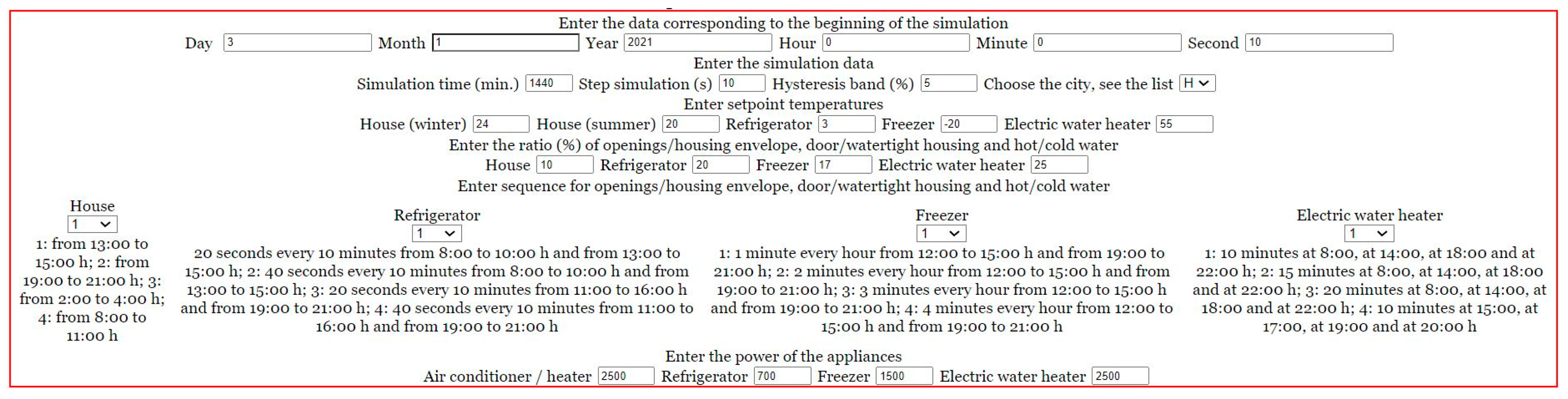
Figure 2.
Flow chart of the developed SBET-TCLs.
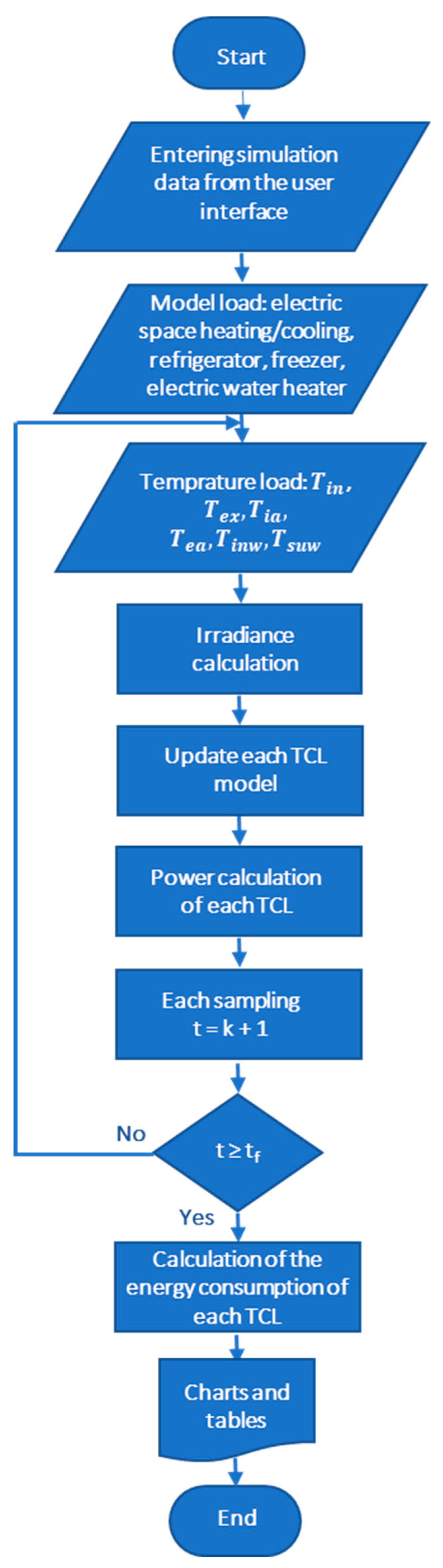
Figure 3.
January 3, 2021. Sequence: 1-1-1-1. Behavior of the space heating/cooling (left) and refrigerator (right).
Figure 3.
January 3, 2021. Sequence: 1-1-1-1. Behavior of the space heating/cooling (left) and refrigerator (right).
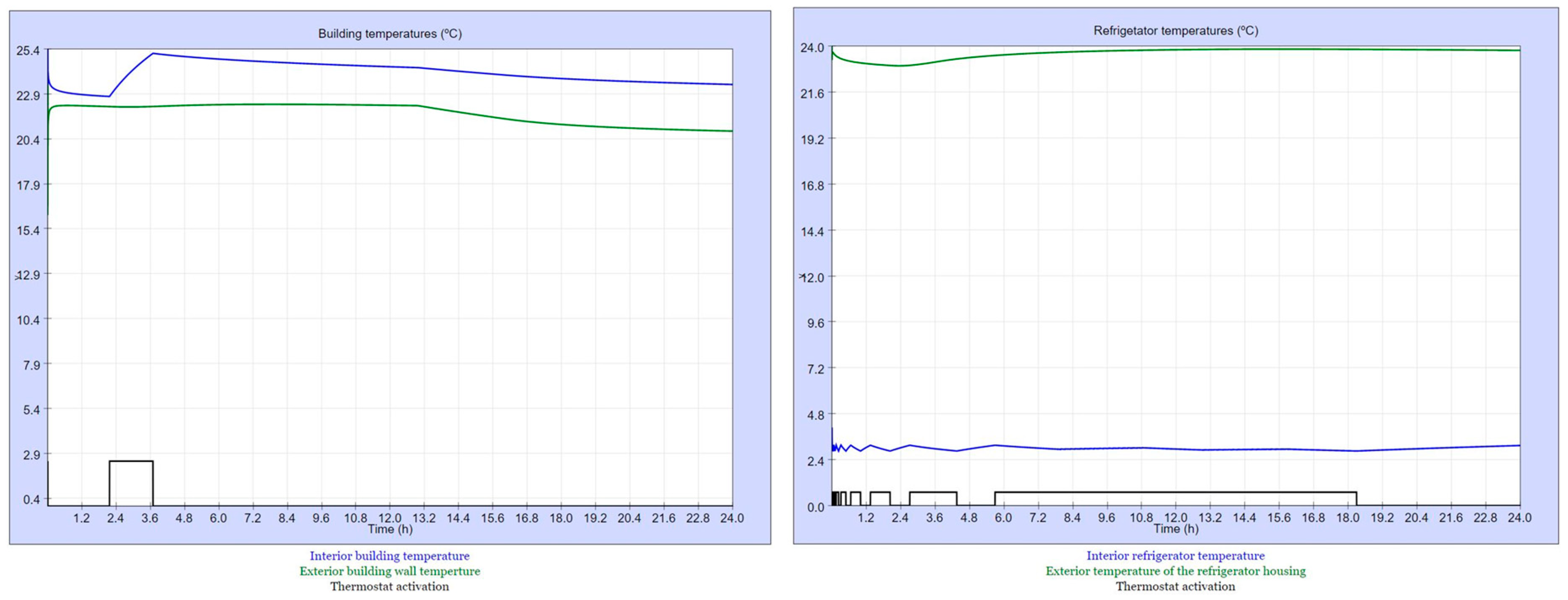
Figure 4.
January 3, 2021. Sequence: 1-1-1-1. Behavior of the freezer (left), water heater (right) and daily consumption down.
Figure 4.
January 3, 2021. Sequence: 1-1-1-1. Behavior of the freezer (left), water heater (right) and daily consumption down.

Figure 5.
January 3, 2021. Daily irradiance.
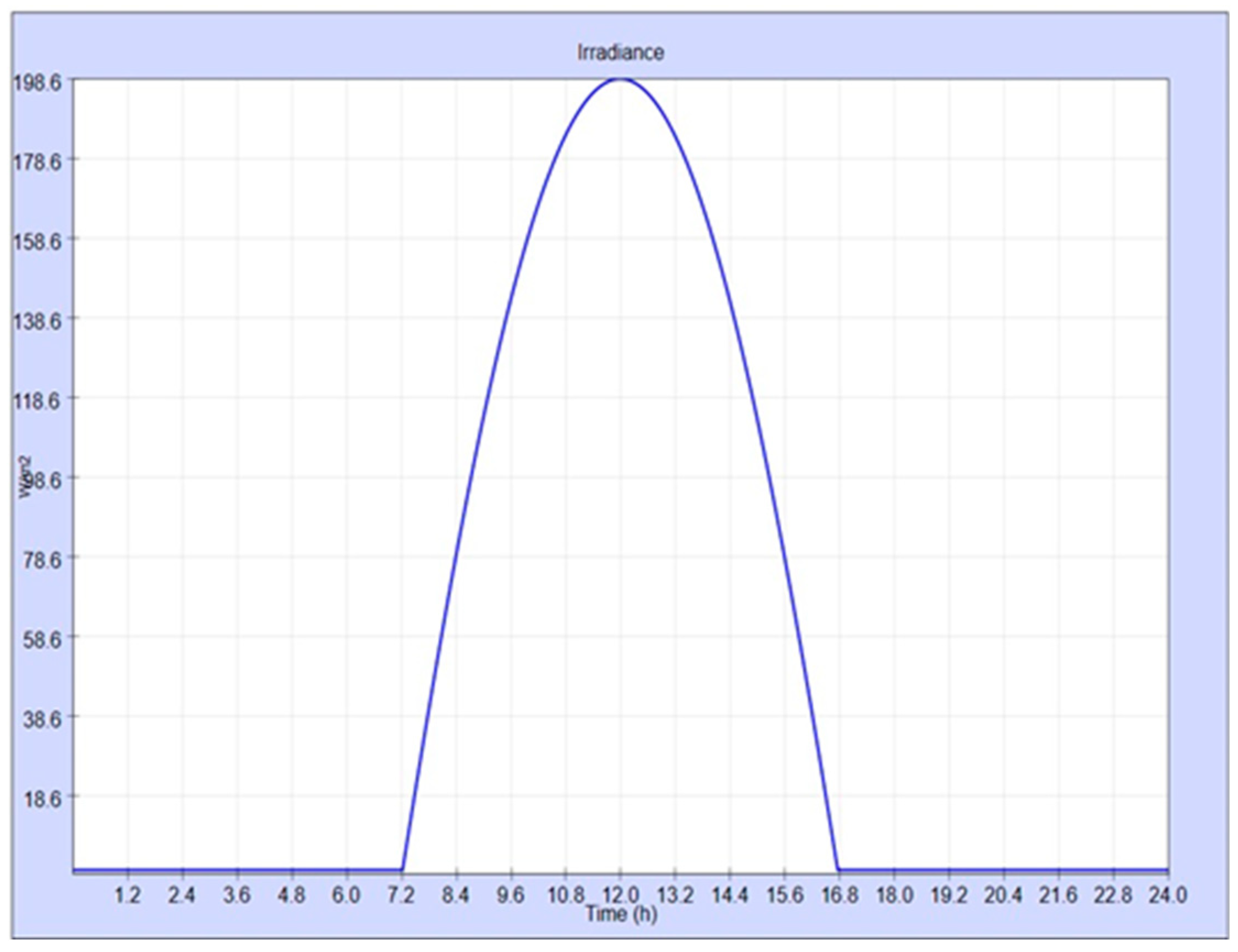
Figure 6.
January 3, 2021. Sequence: 2-4-3-3. Interface of the simulation-based education tool.
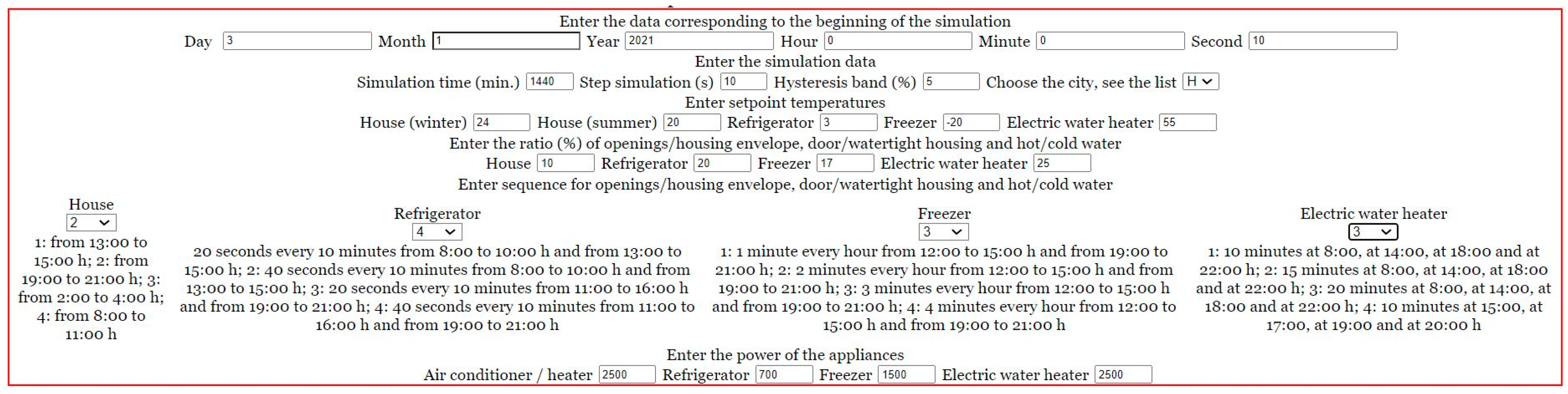
Figure 7.
January 3, 2021. Sequence: 2-4-3-3. Behavior of the space heating/cooling (left) and refrigerator (right).
Figure 7.
January 3, 2021. Sequence: 2-4-3-3. Behavior of the space heating/cooling (left) and refrigerator (right).
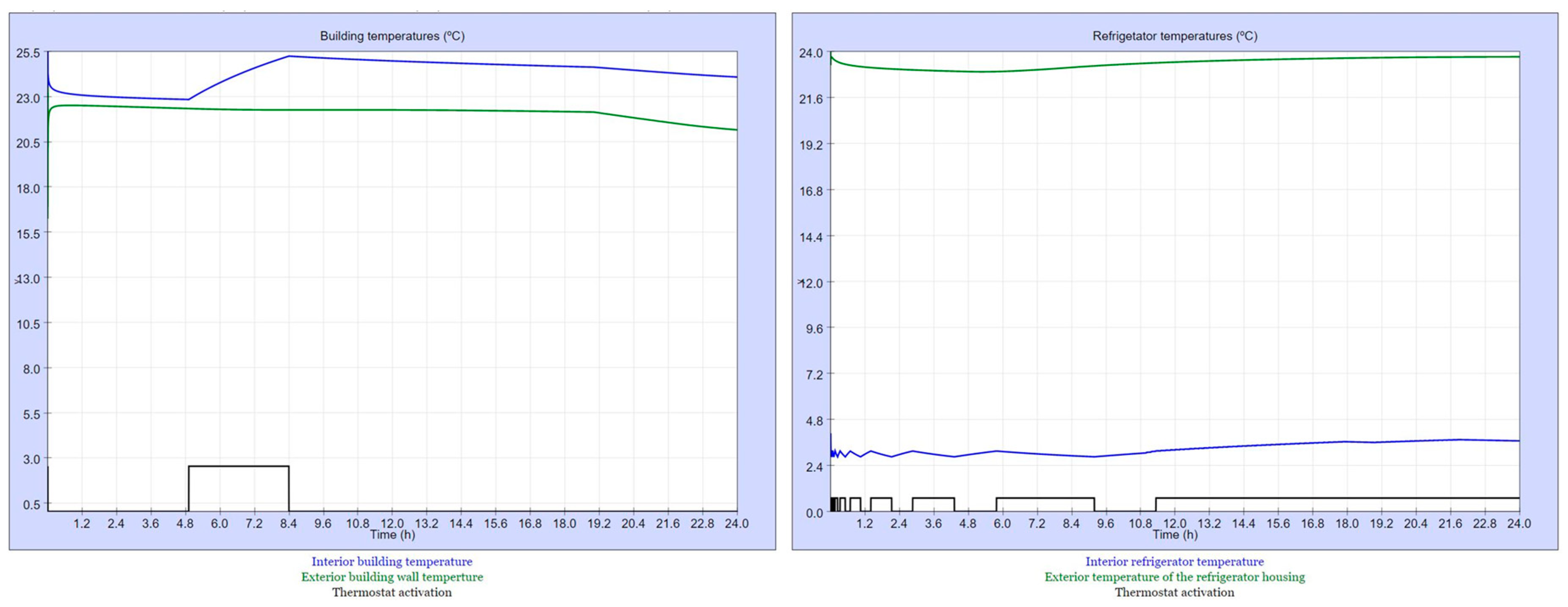
Figure 8.
January 3, 2021. Sequence: 2-4-3-3. Behavior of the freezer (left), water heater (right) and daily consumption (down).
Figure 8.
January 3, 2021. Sequence: 2-4-3-3. Behavior of the freezer (left), water heater (right) and daily consumption (down).
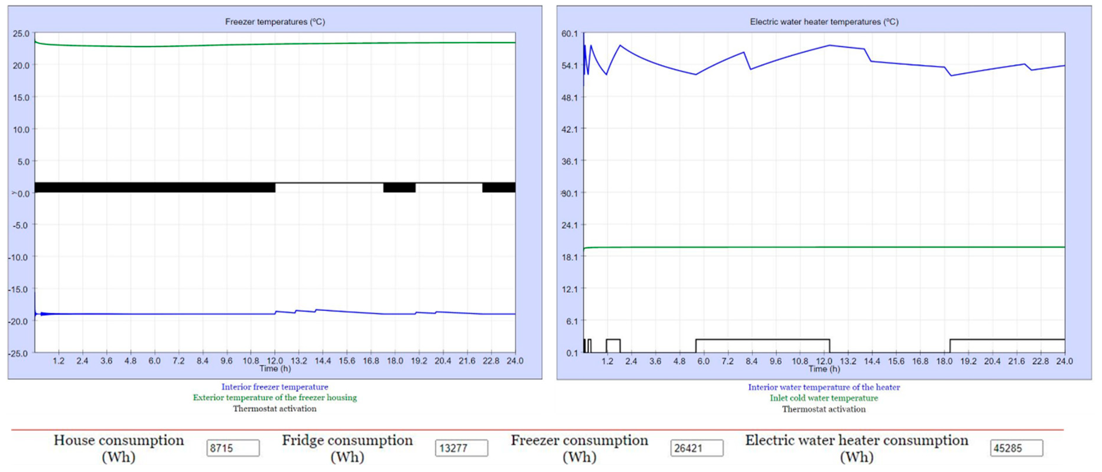
Figure 9.
July 3, 2021. Sequence: 1-1-1-1. Interface of the simulation-based education tool.
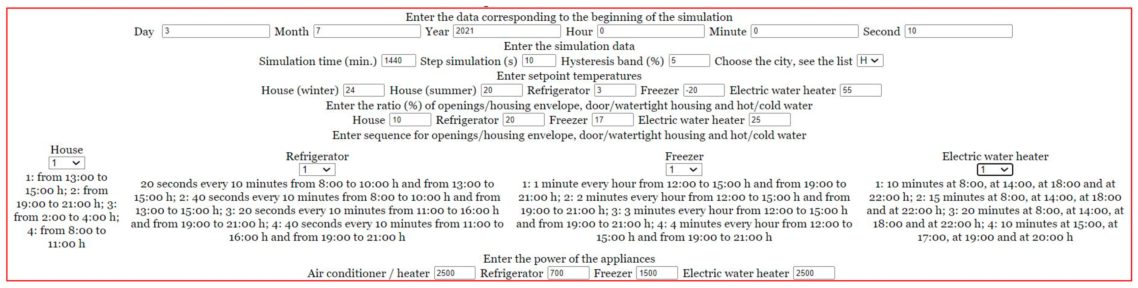
Figure 10.
July 3, 2021. Sequence: 1-1-1-1. Behavior of the space heating/cooling (left) and refrigerator (right).
Figure 10.
July 3, 2021. Sequence: 1-1-1-1. Behavior of the space heating/cooling (left) and refrigerator (right).
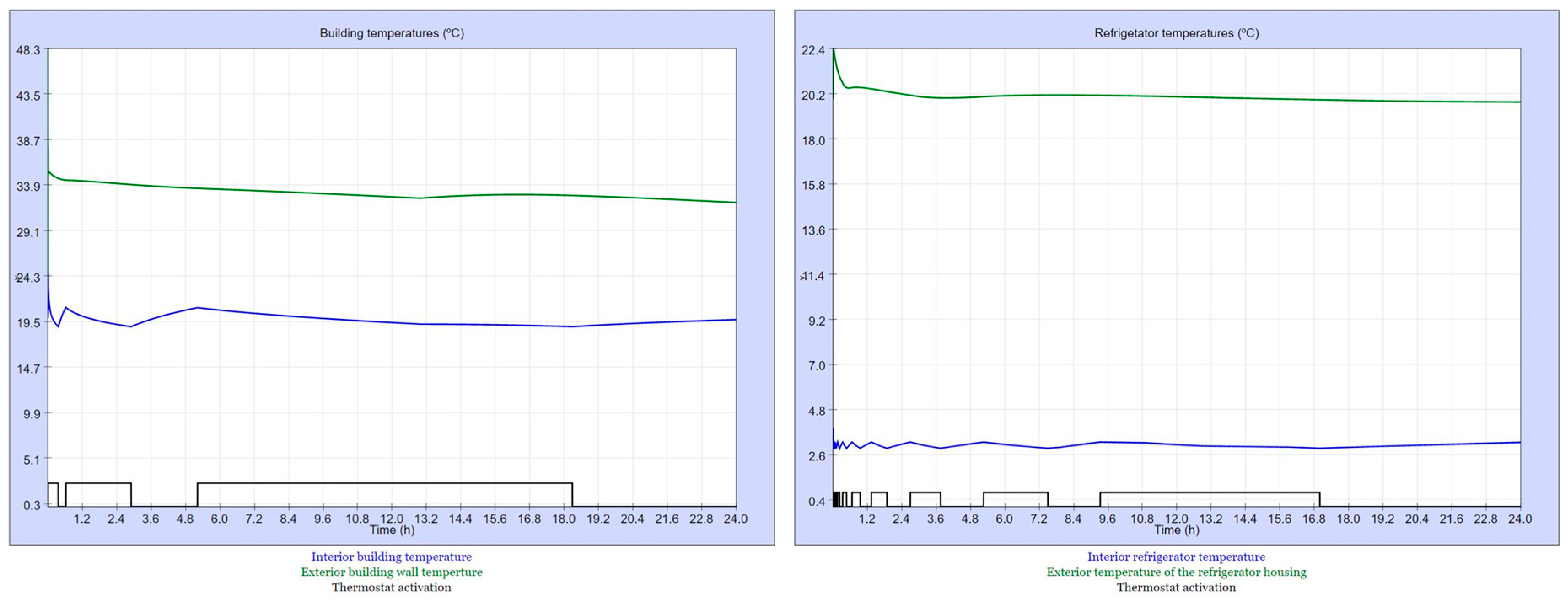
Figure 11.
July 3, 2021. Sequence: 1-1-1-1. Behavior of the freezer (left), water heater (right) and daily consumption (down).
Figure 11.
July 3, 2021. Sequence: 1-1-1-1. Behavior of the freezer (left), water heater (right) and daily consumption (down).
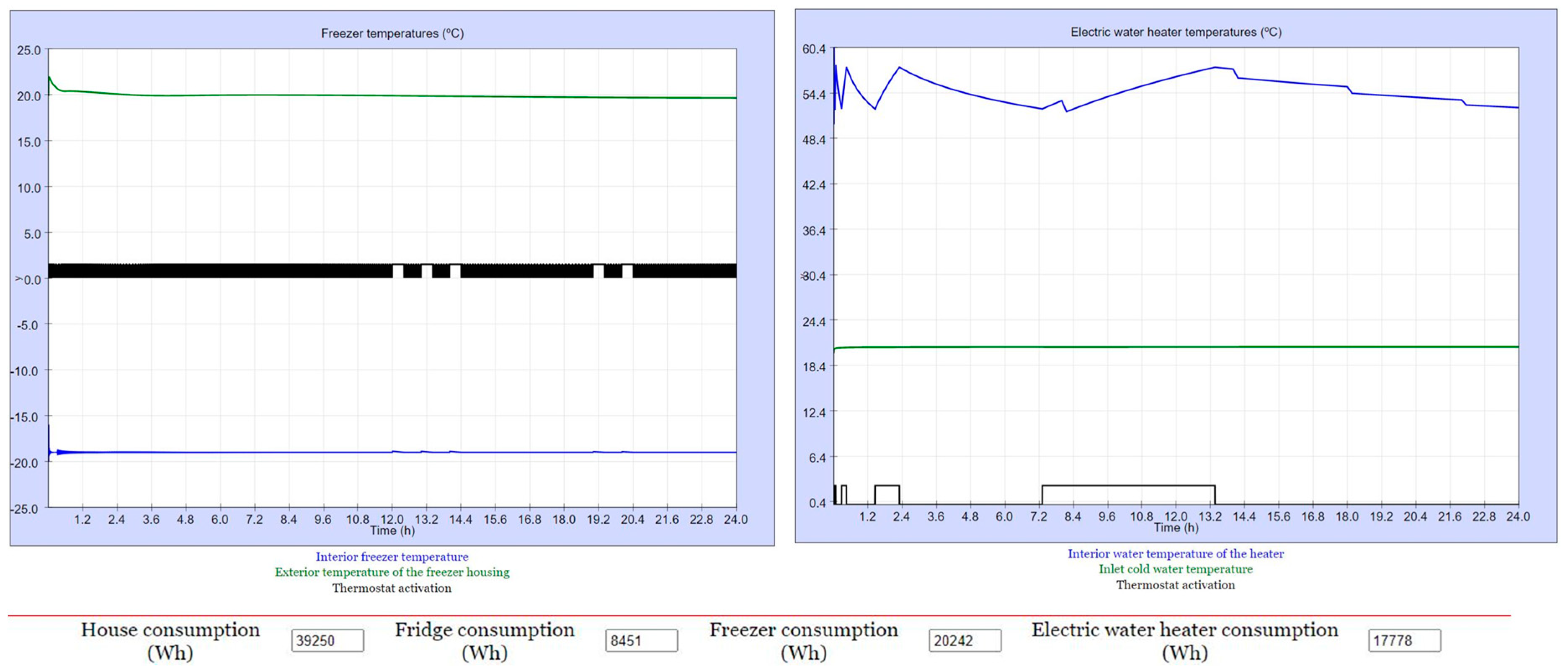
Figure 12.
August 3, 2021. Daily irradiance.
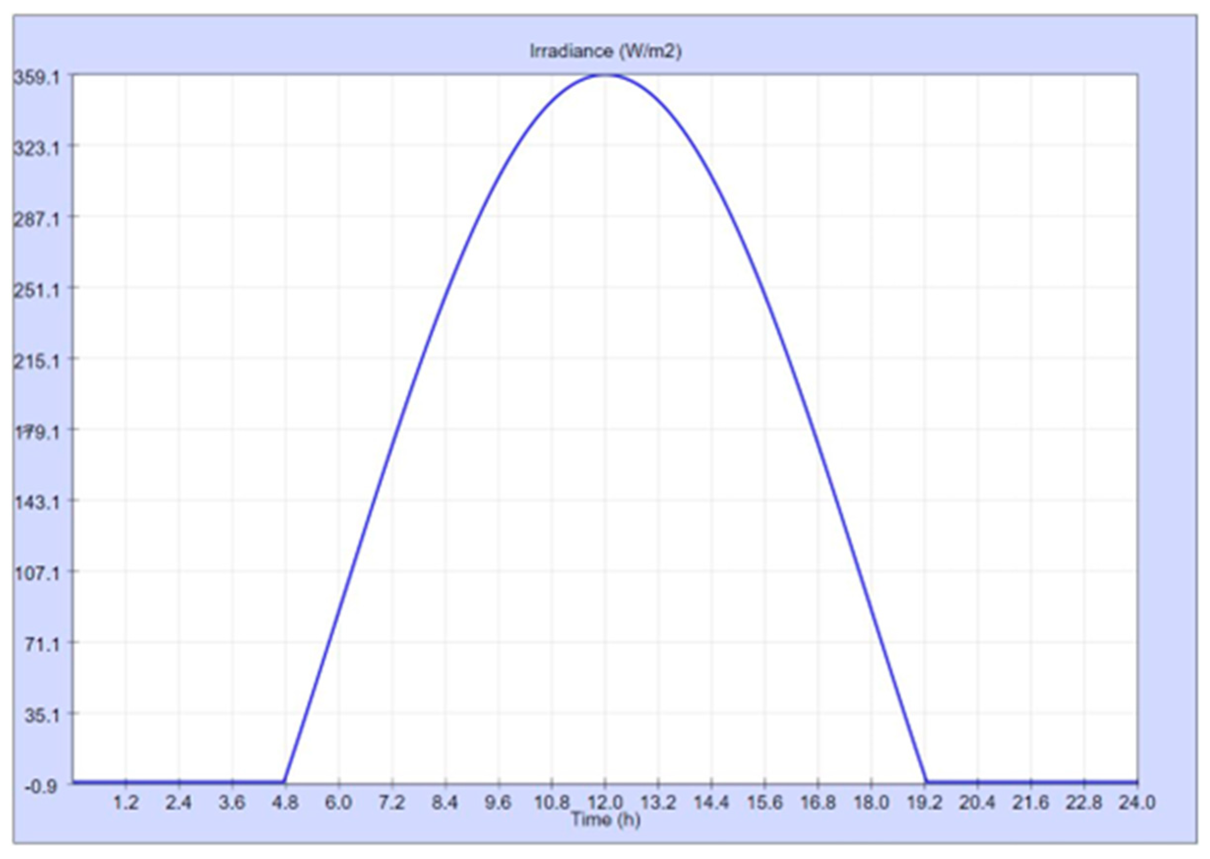
Figure 13.
July 3, 2021. Sequence: 2-4-3-3. Interface of the simulation-based education tool.
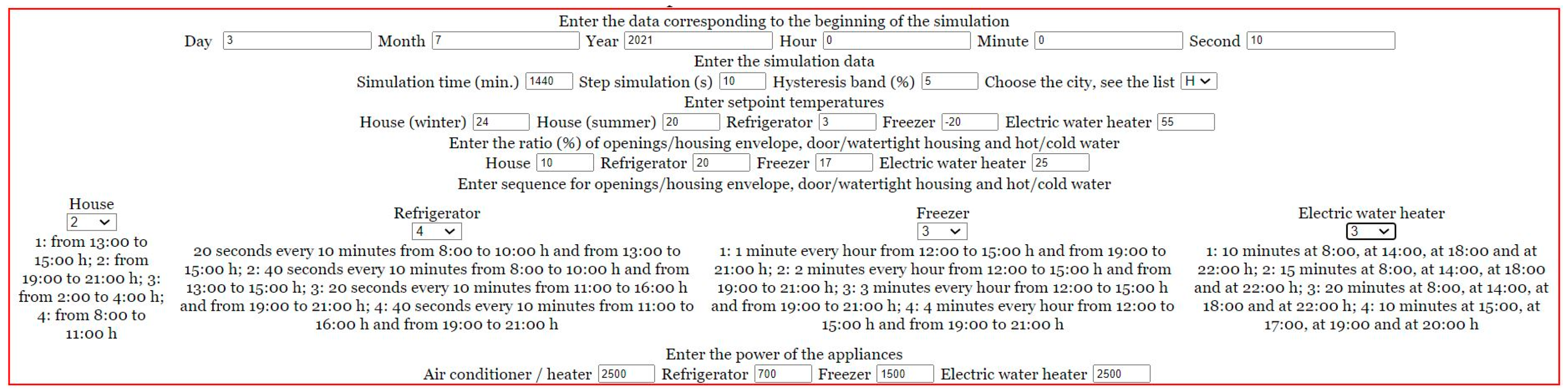
Figure 14.
July 3, 2021. Sequence: 2-4-3-3. Behavior of the space heating/cooling (left) and refrigerator (right).
Figure 14.
July 3, 2021. Sequence: 2-4-3-3. Behavior of the space heating/cooling (left) and refrigerator (right).
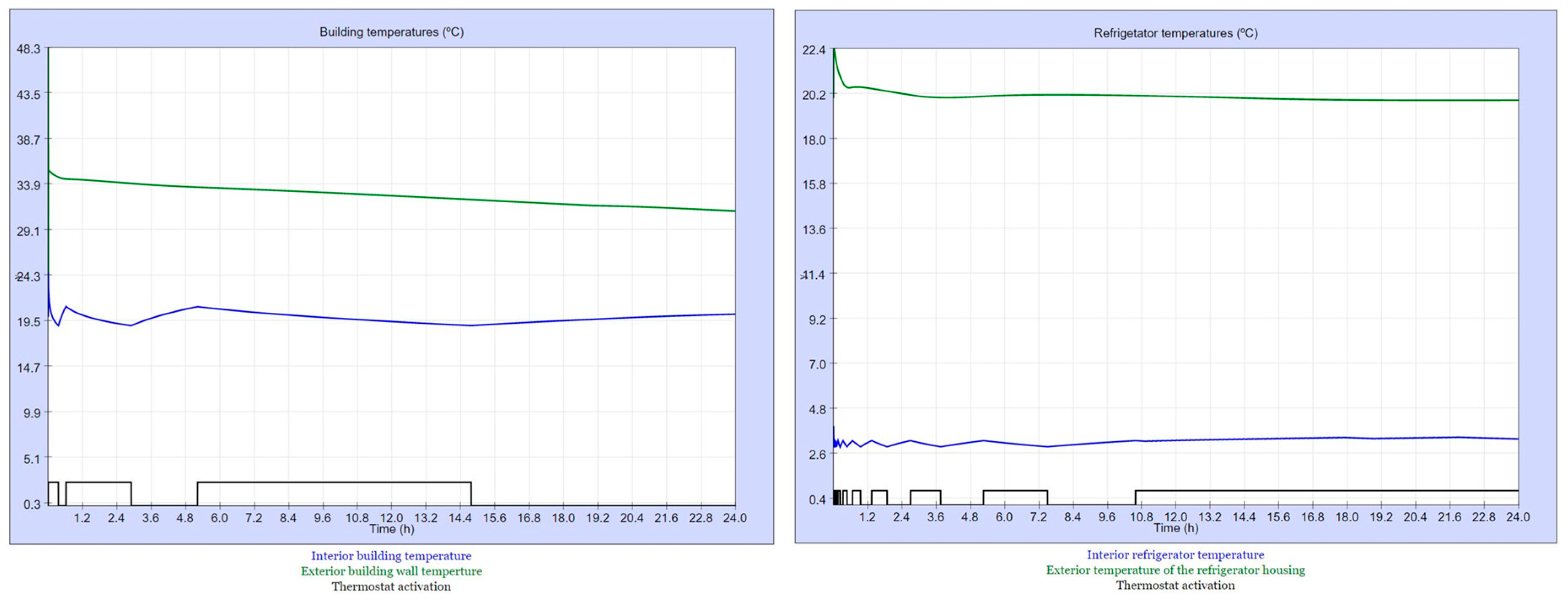
Figure 15.
July 3, 2021. Sequence: 2-4-3-3. Behavior of the freezer (left), water heater (right) and daily consumption (down).
Figure 15.
July 3, 2021. Sequence: 2-4-3-3. Behavior of the freezer (left), water heater (right) and daily consumption (down).

Figure 16.
Evaluation questionnaire of the SBET-TCL as an educational resource.
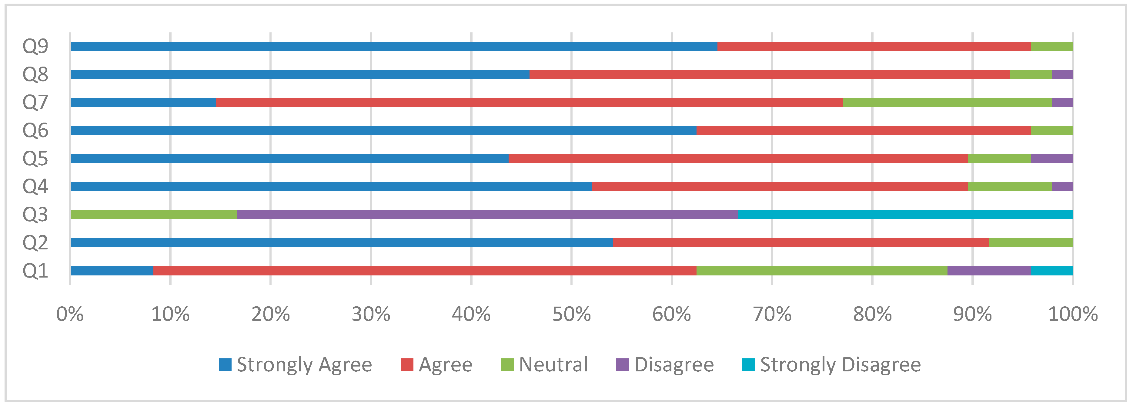
Table 1.
Water supply temperature (°C) in the city of Huelva (southwestern Spain) in 2021.
| Month | Temperature |
|---|---|
| January | 12 |
| February | 12 |
| March | 13 |
| April | 14 |
| May | 16 |
| June | 18 |
| July | 20 |
| August | 20 |
| September | 19 |
| October | 17 |
| November | 14 |
| December | 13 |
Table 2.
Summary of survey.
| Section | Question | Description |
|---|---|---|
| Students’ background | 1 | Your level in ‘Energy Efficiency’ is high |
| SBET-TCLs experience | 2 | The simulation tool allows for the consolidation of theoretical concepts |
| 3 | Theoretical concepts can be learned only through theoretical study | |
| 4 | Computer simulation facilitates theoretical and practical understanding | |
| 5 | Learning is more engaging through the use of the simulation tool | |
| Acceptance of use | 6 | The simulation tool should be used in undergraduate engineering degrees |
| Design quality and ease of use | 7 | The interface is friendly |
| 8 | The simulation tool is easy to use | |
| Overall assessment | 9 | The overall assessment of the simulation tool is positive |
Table 3.
TCL consumption (kWh) as a function of the operating scenario.
| TCL | Sequence | Season | TCL consumption |
|---|---|---|---|
| Space heating/cooling | Sequence 1-1-1-1 |
Winter Summer |
8,715 39,250 |
| Sequence 2-4-3-3 |
Winter Summer |
8,715 36,819 |
|
| Refrigerator | Sequence 1-1-1-1 |
Winter Summer |
11,359 8,451 |
| Sequence 2-4-3-3 |
Winter Summer |
13,277 10,588 |
|
| Freezer | Sequence 1-1-1-1 |
Winter Summer |
22,613 20,242 |
| Sequence 2-4-3-3 |
Winter Summer |
26,421 21,199 |
|
| Water heater | Sequence 1-1-1-1 |
Winter Summer |
25,368 17,778 |
| Sequence 2-4-3-3 |
Winter Summer |
45,285 37,174 |
Table 4.
TCLs simulation input parameters in analyzed cases.
| Simulation Parameter | Unit | Value A | Value B | Value C |
|---|---|---|---|---|
| Hysteresis band | 0.01 | 0.01 | 0.05 | |
| Space cooling setpoint | °C | 24 | 27 | 27 |
| Fridge setpoint | °C | 3 | 3 | 3 |
| Freezer setpoint | °C | -20 | -20 | -20 |
| Electric water heater setpointTotal consumption | °C kWh |
55 96,713 |
55 95,362 |
55 80,419 |
Disclaimer/Publisher’s Note: The statements, opinions and data contained in all publications are solely those of the individual author(s) and contributor(s) and not of MDPI and/or the editor(s). MDPI and/or the editor(s) disclaim responsibility for any injury to people or property resulting from any ideas, methods, instructions or products referred to in the content. |
© 2023 by the authors. Licensee MDPI, Basel, Switzerland. This article is an open access article distributed under the terms and conditions of the Creative Commons Attribution (CC BY) license (http://creativecommons.org/licenses/by/4.0/).
Copyright: This open access article is published under a Creative Commons CC BY 4.0 license, which permit the free download, distribution, and reuse, provided that the author and preprint are cited in any reuse.
Submitted:
06 December 2023
Posted:
07 December 2023
You are already at the latest version
Alerts
A peer-reviewed article of this preprint also exists.
This version is not peer-reviewed
Submitted:
06 December 2023
Posted:
07 December 2023
You are already at the latest version
Alerts
Abstract
Thermostatically controlled loads have great potential to make a significant contribution to improving energy efficiency in the building sector, which is responsible for 40% of greenhouse gas emissions in the EU. This, in addition to the environmental damage, represents a huge expense in the electricity bill. Therefore, it is very important to train engineers on how to design energy management systems for TCLs. With this goal in mind, it would be very useful to have a simulation-based educational tool (SBET) to understand thermostatically controlled loads, their characteristics and possibilities in energy efficiency. In addition, it would be very useful if this tool could be introduced in engineering curricula to help students to be better trained and enter the labor market with more opportunities. Based on the shortcomings detected, this work develops a SBET specifically designed to teach about TCLs (SBET-TCLs), both about their intrinsic characteristics and their better management. To verify the developed SBET-TCL, it has been tested in a real scenario: A survey was carried out among the students of the subject 'Alternative Energy Sources' of the degrees of Industrial Engineering. The results show that the use of SBET-TCL has very positive effects on the learning process.
Keywords:
Subject: Engineering - Electrical and Electronic Engineering
1. Introduction
The current geopolitical situation and the enormous problems of climate change to which the world is subjected, require solutions in the short term to alleviate energy costs on the one hand and, on the other, to begin a gradual process of decarbonization of the planet that will allow at least a glimpse of a future of guaranteed sustainability. Focusing on the electricity sector, it is necessary to decisively address two major problems: reduction of electricity costs (at the end of the chain the bill paid by the user) and increase in the penetration of renewable energies. In this complex scenario, thermostatically controlled loads (TCLs), mainly electric space heating/cooling, refrigerators, freezers, and electric water heaters, have great potential to minimize electricity bills and maximize the penetration of renewables in the electricity system [1]. In fact, heating and cooling loads represent around half of the total energy consumption of EU countries [2]. However, due to the thermal characteristics of the TCLs, by applying appropriate control strategies it is possible to increase or reduce their power, or even make the temporary displacement of TCLs connection without loss of thermal comfort for the user, simply by taking into account the intrinsic thermal storage capacity of the buildings [3]. Thus, to reduce global energy consumption and CO2 emissions in buildings, TCL modeling and control is an excellent resource [4] since it brings a numerous benefits when energy demand is high [5] or energy cost wants to be minimized [6].
Based on the above, despite being a novel field of research, it is necessary to incorporate the management of TCLs in the curricula of students, with emphasis on higher education and engineering careers.
The constant evolution of society and technology implies the need for constant revision of engineering curricula [7]. In engineering education, theoretical concepts are often complex and difficult to bring to real life, thus, practical activities play a very important role in learning. However, open-air activities [8] or real laboratory experiments [9] require expensive equipment, are time-consuming and can involve a certain amount of danger. In particular, teaching TCL control in real laboratories requires complex and expensive equipment, as well as environmental conditions (those corresponding to a real inhabited building: home appliances, insulation, room temperature, etc.) and availability of time of use that are very difficult to achieve.
To overcome the above mentioned drawbacks, simulation-based educational tools (SBETs) can be an excellent choice to complement and enhance the quality of learning about TCLs.
In general, SBETs have been playing an important role in the teaching-learning process for years [10]. Indeed, SBETs have been shown to help both teachers by optimizing educational content, and students by improving comprehension and increasing interest and creativity [11].
There are studies that analyze the learning progress student of groups of students who use SBETs versus those who do not [12]. Results show that groups of students using SBETs have a better learning rate. In fact, according to [13], SBETs allow students to retain up to 90% of educational content, as opposed to reading (10%) or listening (20%).
On the road to place the student at the center of the learning process, novel approaches to learning in science education have emerged in recent years. Examples include collaborative [14], problem-based [15], project-based [16], and competency-based learning [17], along with the flipped classroom [18] and gamification techniques [19], among others. Practices carried out in classroom through these methodologies can be enhanced with different technological applications, resulting in a pedagogical approach known as blended learning [20]. Thus, SBETs are a suitable resource to overcome the challenges and difficulties of the learning process [18,21].
The current digital transformation process has also promoted these new educational approaches. However, until the COVID-19 pandemic, its impact had not been as pronounced as it is now [22,23]. In fact, it is after the COVID-19 pandemic that a European Union (EU) policy initiative known as Digital Education Action Plan (2021-2027) appears, whose aim is to support the adaptation of member states’ education and training systems to the digital age [24].
Perhaps, at the forefront of this transition towards teaching with the student as the protagonist of his own learning process, towards a more digital education are the universities [25]. In this framework, students’ interest and motivation increase, and the development of their skills is facilitated.
SBETs can be self-developed [26,27,28] or commercial [29,30,31,32], and involve virtually all engineering degrees. In this way, there are applications in electrical [33], electronic [34,35], communications [36], control [37,38], computer science [39], thermal energy [40] or mechanic [41], among others.
Focusing on the field of TCLs, there are some simulation-based tools in the literature that can manage them [42,43,44,45,46], but not specifically, but as part of a network, usually an electrical network. Moreover, although these tools can be used in educational environments, they are not developed for that purpose, so, among other things, they lack the necessary utilities to deepen the intrinsic knowledge of TCLs. Therefore, and in this sense, they cannot be considered SBETs. Thus, GridLAB-D™ [42] was developed by the U.S. Department of Energy (DOE) and envisions the management of TCLs as just another load in an electrical distribution system. On the other hand, the Object-oriented, Controllable, High-resolution Residential Energy (OCHRE) tool [43] does not deal in a specific way with TCLs but can include them in its simulations as thermal loads. As for OpenDSS [44], it is an electrical power distribution system simulator that can handle TCLs as loads with specific hourly operation, but not as a control system to optimize them. Finally, [45,46] are designed for the microgrids simulation. Thus, RAPSim (Renewable Alternative Powersystems Simulation), [45], is a free and open source microgrid simulation framework whose main objective is to foster the understanding of power flows in smart microgrids with renewable sources. Again, TCLs are just another load. With regard to [46], HOMER Pro® microgrid software by HOMER Energy is a high-level simulation payment framework. Its capabilities are enormous, but it does not delve, or even go into, the nature of TCLs as they are of interest in an academic setting.
After analyzing the state of the art of the availability of SBETs in the literature for the in-depth study of TCLs, it was concluded that there were no tools suitable for academic environments. Consequently, this was the motivation for the work presented in this article: a specific SBET for TCLs (SBET-TCLs).
This paper presents a SBET-TCLs that allows to study in depth the dynamic behavior, energy consumption and best management of the TCLs in buildings (in the following and throughout the paper, building, house or dwelling may be used interchangeably) applications: electric space heating/cooling, refrigerators, freezers, and electric water heaters. Due to the experience in previous developments, the simulation tool was implemented using Easy Java/JavaScript Simulations (EJS) [47], an open source tool written in Java, mainly dedicated to teaching and learning purposes.
The main objective of this research is to improve, through the development and use of a new SBET, the learning of TCLs, facilitating their understanding and practical applicability. Then, following the line of previous education works of the authors and aiming to measure the suitability of the proposed SBET, a survey has been carried out among the students of the subject ‘Alternative Energy Sources’ of the degree courses in Electrical Engineering, Industrial Electronic Engineering, Mechanical Engineering and Industrial Chemical Engineering. Results show that the use of the developed SBET improves the learning process on TCLs in these degrees.
Based on everything discussed in this section, this paper is novel for the following reasons:
(1) Prior to the proposed SBET, there were no tools suitable for academic environments specifically focused on the TCLs teaching/learning process.
(2) The proposed SBET delves deeper into the intrinsic behavior of TCLs, i.e., it allows them to be studied at the lowest level.
(3) The proposed SBET allows modeling TCLs as state space models, which captures their dynamics.
(4) The proposed SBET works with parameterized models that can be easily modified by the student according to the application under study.
(5) The proposed SBET is a very intuitive and easy framework, which is essential in an educational environment, otherwise the student will be demotivated by the workload.
(6) The proposed SBET has been incorporated into curricula and tested in real engineering degree scenarios.
(7) To the authors’ knowledge, there is no TCL model in the literature that is more intuitive, simpler, and easier to calculate and interpret than the one presented in this article.
The remainder of this paper is organized as follows. Firstly, the article presents the theoretical framework and the methods to know some necessary parameters in the developed models in Section 2.1 and Section 2.2, respectively. Then, the educational framework is described in Section 2.3. A description of the developed simulation-based educational tool is given in Section 3. Next, the results about the technical performance of the developed simulation-based educational tool and their evaluation as an educational resource are reported in Section 4.1 and 4.2, respectively. Results obtained are discussed in Section 5. Finally, some conclusions are drawn in Section 6.
2. Materials and Methods
The materials and methods used in the SBET development can be divided into two distinct parts. The first one refers to the technical aspects of the tool, that is, what is its scientific basis thermodynamically speaking. The second refers to the educational aspects of the tool, that is, its evaluation as an educational resource.
2.1. Theoretical framework of the developed simulation-based education tool
As already explained, the usual TCLs in a building are considered in the study: electric space heating/cooling, refrigerators, freezers, and electric water heaters. Each TCL is modeled following an approach known as grey-box model [48], which are dynamic thermal models (state-space models) identified from experimental measurements [49]. The main concept of the grey-box models is to group and represent the different components of the TCLs by means of thermal resistances (R), representing the difficulty in the heat transfer (i.e. the degree of tightness of the thermal enclosures), and thermal capacities (C), which represents the capacity to store energy in the form of heat. This is analogous to the way an electrical circuit hinders the passage of electric current through resistors and stores electrical energy through capacitors. As a simple example, consider a building in which air infiltration losses through the windows are not taken into account, nor the temperature difference between the ambient temperature and that of the walls. In this case, any room with exterior walls has two thermal nodes (interior and exterior wall surface) with their respective thermal capacities connected by a thermal resistance representing the rate of convective and radiative heat exchange between them through the wall.
This type of RC model must be identified, i.e., applied to the example of the building, the different values of R and C in the different parts of the building due to the different TCLs have to be calculated or measured [50]. The value of C depends on the node’s ability to store energy in the form of heat; think, for example, of the outer surface of a wall that absorbs energy depending on the solar radiation, its color and physical composition. Regarding R, the higher the thermal insulation of the wall, the higher its value because it opposes the heat transfer between the nodes representing the internal and external surfaces.
Models are formulated using the discrete time state-space representation. In the linear case as in (1) - (2); developed from [51].
The state equation (1) is the result of the thermodynamic analysis of the TCL, which leads to a system of as many first-order differential equations as there are energy storage elements in the model (thermal capacities). As for the output equation (2), it can be observed that it has not dynamic and is decided by the designer, usually with an output vector with as many coordinates as variables of interest that can be measured.
In detail, is the sampling, is the state vector, the order of the model (the number of first-order differential equations), is the input vector, where p is the number of inputs, is the state matrix, the input matrix, and the vector of m model parameters. Note that the parameter vector depends on discrete time because the TCL conditions can vary with time; think for example of an open/closed window or open/closed refrigerator door (please, see Appendix).
As for the output equation (2), is the output vector, where q is the number of outputs, and is the output matrix.
Next, based on the physical principles established so far, the state space models for each TCL included in the proposed SBET will be developed.
2.1.1. Electric space heating/cooling
The development of this model is based on [49]. The state, input and output vectors of the model are written, respectively, in (3).
Where the state vector is make up by the temperature at each thermal node due to the corresponding thermal capacity, three in this case: the interior building wall temperature , the exterior building wall temperature , and the indoor air temperature or interior ambient temperature due, respectively, to the thermal capacities , and . This model considers the interior ambient temperature as a separate temperature node of the interior building wall temperature node , which adds accuracy to the model because, in general, the ambient temperature and the wall temperature are different. Regarding the input vector , it is make up by the variables that force the temperature changes of the building. These are the outside building air temperature or exterior ambient temperature (this model considers the exterior ambient temperature different from the exterior building wall temperature since in general both are different; again, this adds accuracy to the model) that influences by the wall thermal conduction and the opening of doors and/or windows, electrical power consumed by the building for heating/cooling and irradiance , or energy per unit area of global solar radiation incident on a horizontal surface of the building. It is calculated according to the position and orientation of the building, as well as its geographical location (latitude and longitude) [52]. Finally, the output vector coincides with the state vector (this facilitates the use of the state vector for controller design because all its coordinates can be measured [53]) and represents the evolution of the temperatures of each of the thermal nodes. The model matrices are (4) - (6).
Where , , and are, respectively, the thermal resistances between nodes and , and , and , and . Thus, following (1) - (2), , , , , , ; values of these model parameters are listed in Table A1 of Appendix A. Finally, numerical values ( and ) can be observed in matrix B, whose meanings are coefficients to fit the model.
In what follows, the meaning of the subscripts of the variables is the same for the rest of models. Of course, taking into account in each case the physical environment of each TCL.
2.1.2. Refrigerator
The development of this model is based on [54]. The state, input and output vectors of the model are written, respectively, in (7).
Where the state vector is make up by the interior refrigerator temperature and the exterior temperature of the refrigerator housing due, respectively, to the thermal capacities and . In this case, due to the interior volume of the refrigerator housing (considerably lesser than that of a room in a building) and its degree of thermal insulation (considerable larger than that of a room in a building) both the interior ambient temperature and the temperature of its interior walls are considered to be the same,. As for the input vector , it is make up by the variables that force the temperature changes of the refrigerator: air temperature around the refrigerator, i.e., the interior ambient temperature of the building (this model considers the exterior ambient temperature around the refrigerator housing different from the exterior temperature of the cooler housing since in general, both are different; this adds accuracy to the model) that influences by the refrigerator housing thermal conduction and the opening of its door, and the electrical power consumed for cooling . Finally, the output vector coincides with the state vector and represents the evolution of the temperatures of each of the thermal nodes. The model matrices are (8) - (10).
Where , , and are, respectively, the thermal resistances between nodes and , and , and . Thus, following (1) - (2), , , , ; values of these model parameters are listed in Table A2 of Appendix A.
2.1.3. Freezer
Following [55], the model of the freezer is analogous to that of the refrigerator, i.e. (7) – (10). Now power consumed for cooling is . Model parameters values are listed in Table A3 of Appendix A.
2.1.4. Electric water heater
The development of this model is based on [56]. The state, input and output vectors of the model are written, respectively, in (11).
Where the state vector is make up by the interior water temperature of the heater and the exterior temperature of the water heater housing due, respectively, to the thermal capacities and . As for the input vector , it is make up of the variables that force the temperature changes of the water in the heater: temperature of cold water supplied to the heater (when the water heater is receiving water from outside to compensate for the water it is supplying) and the electrical power consumed for heating . Faced with these input coordinates with a great influence on the changes in water temperature in the heater, thermal conduction of the heater housing is not taken into account (the water heater will normally be inside a cabinet and the heat exchange with the outside can be considered negligible compared to the daily inflow of cold water). Again, the output vector coincides with the state vector and represents the evolution of the temperatures of each of the thermal nodes.
Changing the corresponding subscripts and values, matrix A is the same as in (8), matrix B is the same as in (9), and matrix C is the same as in (10). Model parameters values are listed in Table A4 of Appendix A.
2.2. Temperature and irradiance measurement
As can be seen in the models of the Subsection 2.1, to calculate the electrical power consumed by the TCLs
it is necessary to have continuously available interior and exterior ambient temperatures to the building, interior and exterior wall temperatures as well as the irradiance to which the building is exposed. In addition, for the refrigerator and freezer, it is necessary to know the internal and external temperatures of their housings. Finally, as far as the electric water heater is concerned, it is necessary to know the temperature of the water inside it and the inlet temperature coming from the supply to the building.
In general, obtaining temperature values is very simple, since it is enough to have thermometers for this purpose (many household appliances supply them directly; [57] is a very accurate and inexpensive device for measuring surface temperatures as in [58]), and even the ambient air temperature outside the building can be obtained directly from the weather stations available in all cities (in the larges there are usually different measurement points, which logically allows it to choose the closest one). The same applies to the temperature of the water stored inside the water heater (provided by the device itself). There are even water heaters that provide information on the inlet water temperature from the exterior. In any case, water supply companies provide graphs of water supply temperatures. For example, in the city of Huelva (southwestern Spain), the monthly supply temperatures for 2021 are shown in Table 1 [59].
That said with respect to the ease of measuring temperatures, the same does not apply to irradiance. The device for measuring solar radiation on a flat surface (irradiance) is called a pyranometer. It is an expensive meter that, in addition, requires special care in positioning for reliable measurements. Therefore, it is not easy, much less usual, for every building to have one. For this reason, the developed SBET-TCL calculates the irradiance instead of measuring it, for which equation (12) is used, which has been adapted from [60].
Where:
is the received irradiance in between the initial time and the final time considered.
is the solar constant or total solar irradiance, i.e. the total amount of energy received as solar radiation per unit time and area measured outside the Earth’s atmosphere in a perpendicular plane to the sun’s rays. The measured and accepted value is .
is the correction factor of due to the eccentricity of the Earth’s orbit around the sun [61]. Specifically, , where is the number of days between 1 (January 1) and 365 (December 31).
is the latitude of the building under study.
is the solar declination resulting from the tilt of the Earth’s rotation axis. The value of solar declination varies continuously throughout the year, from a maximum of at the boreal summer (austral winter) solstice to a minimum of at the boreal winter (austral summer) solstice, where is the obliquity of the ecliptic. Solar declination is zero at the spring and autumnal equinoxes. .
is the solar angle, 0 at noon, negative in the mornings, and with a variation of 15° per hour from noon on. Then, between and varies between and , respectively. Finally, is the number of days between 1 (January 1) and 365 (December 31).
2.3. Educational framework of the developed simulation-based education tool
The study involved undergraduate engineering students of the subject ‘Alternative Energy Sources’. In this subject, students learn about the most commonly used renewable energy sources and energy demand management. Within this last topic, concepts and applications of TCLs are presented. Until the incorporation of the proposed SBET-TCLs, teachers were teaching the TCL framework in a theoretical way, and there was no measure of the students’ learning progress in this scope, other than theoretical assessment.
To measure the suitability as an educational resource of the proposed SBET-TCLs, students were asked to fill out a questionnaire with a set of questions on a 5-point Likert scale (1 = strongly disagree and 5 = strongly agree). The questionnaire was organized in different sections, focusing on the students’ level of knowledge of the subject, and on computer simulation-based learning, as well as on aspects of acceptance, design and usability of the simulation tool together with general considerations. Table 2 shows the survey questionnaire. To conduct this survey, a total of 48 students of the subject ‘Alternative Energy Sources’ (fourth-year elective) from the undergraduate degrees in Electrical Engineering (21% of students), Industrial Electronic Engineering (21%), Mechanical Engineering (29%), and Industrial Chemical Engineering (29%) were asked. The study was carried out in the second semester of the 2021-2022 academic year. The questions listed in Table 2 were asked to the students during laboratory sessions, when the teacher was already aware that they had understood the necessary theoretical concepts about the TCLs.
3. Developed simulation-based education tool
In the following, the developed SBET-TCLs will be explained, both its internal structure and its interface and capabilities.
Figure 1 shows the interface that the student can see when accessing the tool through a XHTML page. The interface is very simple, intuitive, and easy to use. The student must enter the data and parameters corresponding to the desired simulation. Specifically, in the first line: the corresponding date (day, month and year) and the start time (hour, minute and second). In the example in Figure 1, January 3, 2021, 10 seconds after midnight.
In the second line, the simulation data must be entered: simulation time in minutes, step simulation in seconds, hysteresis band percentage (it is a percentage of the set point temperatures, i.e., in a real situation it prevents the respective thermostats of the appliances from switching on and off continuously) and the city where the building is. In the example shown in Figure 1 and by the same order: 1,440 min (24 h), samples every 10 s, allowable percentage of 5% temperature variation from the set point temperature and, finally, the city of Huelva (southern Spain) for the location of the building.
The third line includes the set points for the temperatures (°C) of the different TCLs, i.e., the winter and summer comfort temperatures in the building, as well as the refrigerator, freezer and electric water heater. In the example shown in Figure 1 and by the same order: 24 °C (this means that with the chosen hysteresis band (5 %), and taking into account that it is a winter day, the interior temperature of the building can drop up to 22.8 without activating the electric space heating; of course, the same applies to all other set point temperatures listed below), 20 °C, 3 °C, -20 °C and 55 °C.
The fourth line allows to take into account the variation of the thermal resistances due to the opening of doors and/or windows (building), doors (refrigerator and freezer), and the contact of the incoming cold water with the internal hot water each time the electric water heater is used (outgoing hot water is replenished with incoming cold water). The meaning of the ratio (%) of openings/housing envelope, door/watertight housing and hot/cold water is as follows in each case: surface area of the open doors and/or windows in relation to the surface area of the envelope of the building, surface of the open door in relation to the refrigerator and freezer watertight housing and, finally, in the case of the electric water heater is the percentage of stored hot water consumed in each use. In the example shown in Figure 1 and by the same order: 10% (sum of the doors and/or windows) of the total envelope of the dwelling is open to the exterior, 20% (the surface of the refrigerator door is one-fifth of its total watertight enclosure), analogous to the freezer but now only 17% and, finally, 25 % means that for each shower, one-quarter of the total hot water stored in the electric water heater is used and, subsequently, replaced by cold water.
The user can decide on the fifth line at what times and for how long the doors and windows of the building, the refrigerator and freezer door will be open, as well as how the water heater will be used. Of course, as for the use of the appliances, the casuistry can be infinite, so the tool offers only some representative options. In fact, what is really intended is that the student learns to know how the different types of uses affect consumption so that he/she can apply responsible use. In the example shown in Figure 1 the sequence is 1-1-1-1.
Finally, the last line of the interface allows to introduce the power (W) of the appliances that represent the TCLs; in the case of Figure 1: air conditioner/heater (2,500 W), fridge (700 W), freezer (1,500 W) and water heater (2,500 W).
The developed SBET-TCL was implemented by Easy Java Simulations (EJS) [47], an open-source tool written in Java, mainly for teaching and learning purposes. During the last decade, EJS has been widely used in educational research in engineering, specifically in automatic control [62], robotics [63] and automation [64] among others. Moreover, after years of implementation and use of remote laboratories in higher engineering studies, the authors of this work have already achieved sufficient experience with this tool.
As for the structure of the developed SBET-TCL, it is shown in Figure 2 and will be explained below. First, the tool loads the data entered by the user through the interface of Figure 1. Then loads the models with their parameters (Subsection 2.1 and Appendix A, Table A1, Table A2, Table A3 and Table A4). To these, the temperature data are added. From here, the irradiance is calculated by (12). Now, once the models have been updated, the consumed power by each TCL can be calculated. In this sense, the algorithm takes into account the hysteresis band selected by the user, as well as the setpoint temperature of each TCL. If this is within the hysteresis band, the corresponding TCL does not consume power.
The algorithm runs in a loop until the end of the simulation time () chosen by the user in the interface (Figure 1). Note that temperatures should be updated at each sampling. The same is true for the model parameters, which will be updated depending on the user’s choice (Figure 1) of the sequence for openings/housing envelope, door/watertight housing and hot/cold water. For that, the algorithm loads the proper data (please see Appendix A, Table A1, Table A2, Table A3 and Table A4) of , and . When the algorithm goes out of the loop, the chosen simulation time has finished and the integration of the power over the simulation time delivers the energy consumed. As will be seen in the following section on results, the SBET-TCL provides a set of graphs and tables that allow a detailed analysis of consumption.
4. Results
In this work, the results are of two types, namely, those due to the technical performance of the developed SBET-TCL and those corresponding to the evaluation of the SBET as an educational resource.
4.1. Technical performance of the developed SBET-TCL
In order to obtain sufficient variability when displaying the results of the developed SBET-TCL, a winter day and a summer day have been chosen. For both, two different sequences (1-1-1-1 and 2-4-3-3) for openings/housing envelope, door/watertight housing, and hot/cold water (please, see Figure 1) have been taken into account. A total of four simulations were carried out.
The following figures (Figure 3, Figure 4, Figure 5, Figure 6, Figure 7, Figure 8, Figure 9, Figure 10, Figure 11, Figure 12, Figure 13, Figure 14 and Figure 15) show the behavior of the appliances regarding the interface set by the user and the environmental conditions of the dwelling. In the figures mentioned above, the indoor and outdoor temperatures are shown in blue and green, respectively, and the activation of the thermostat of each device and, consequently, the power consumption (always considering the nominal one), are in black.
Table 3 summarizes the energy consumption in each of the four scenarios considered.
Day: January 3, 2021. Sequence: 1-1-1-1. Its interface corresponds to that shown in Figure 1. Results are shown in Figure 3, Figure 4 and Figure 5.
Day: January 3, 2021. Sequence: 2-4-3-3. Its interface corresponds to that shown in Figure 6. Results are shown in Figure 7 and Figure 8. Of course, the daily irradiance is that of Figure 5.
4.2. Evaluation of the SBET-TCL as an educational resource
Students in the ‘Alternative Energy Sources’ course have evaluated SBET-TCL in the scenarios shown in Subsection 4.1. Among others designed by themselves, and with the objective of making them to realize the need of controlling TCLs, the test indicated in Table 4 has been proposed. As can be seen, it consists of three simulations. The first one is the base case with the parameters indicated in Figure 9, except hysteresis band. In the second one, all the parameter and kept constant except the building set point, which is increased from 24°C to 27°C. The parameters corresponding to the third simulation are the same as the corresponding to the second one, except the hysteresis band, which has been highly increase. The rest of initial parameters not included in Table 4 are the corresponding to Figure 9. The total consumption obtained in each case is presented in Table 4.
Now, once checked the technical suitability of the developed tool was time to check its educational suitability. For this purpose, the survey designed in Table 2 was carried out. The result is shown in Figure 16. Q1-Q9 represent, respectively, the questions indicated in Table 2, Section 2.3.
5. Discussion
5.1. Technical performance of the developed SBET-TCL
The SBET-TCL developed in this work constitutes a very good tool for students of different degrees and qualifications to learn the operation of TCLs as well as the need for their control to reduce their electrical consumption. Regarding fridge and freezer, the curves representing the evolution of the different temperatures are very similar in summer and winter because their operation mainly depends on the ambient temperature in the place that they are located. Thus, their consumption is higher in winter, when the building temperature set point is higher than in summer. In addition, their consumption is higher as higher is the time involved in “openings/housing envelop, door watertight/housing and hot/cold water”. I.e., the consumption corresponding to 2-4-3-3 sequence is always higher than the corresponding to 1-1-1-1.
With respect to the electric water heater, it must be observed in Table 3 that the consumption corresponding to the summer is lower that the winter. This is consequent because the inlet winter temperature is lower than the corresponding to the summer. In addition, the consumption corresponding to the 2-4-3-3 sequence is about the doble of the corresponding to 1-1-1-1 as the time of using hot water in the second case is about the middle of the first.
Finally, regarding the building, the consumption is much higher in summer, as correspond to a place with a hot weather. The consumption corresponding to the sequence 2-4-3-3 is higher than the corresponding to 1-1-1-1 in summer. In winter, consumptions corresponding to both sequence is the same although in the curves that show the evolution of the temperatures (Figure 3a and Figure 7a) it can be seen a little difference.
Simulations whose results are presented in Table 4 show to the students the importance of controlling the TCL parameters to limit their consumption.
5.2. Evaluation of the SBET-TCL as an educational resource
Regarding to suitability as a SBET-TCL, results show positive general assessment (question 9). The level of knowledge of the students involved in the SBET-TCL evaluation about “Energy Efficiency” is considered high (question 1) and it is because the theoretical concepts related to TCL were earlier taught in theory classes. With respect to SBET-TCL experience, students agreed that theoretical concepts are strengthened and learning procedure is improved with the simulation platform (questions 2, 4 and 5). Otherwise, they did not think that theoretical concepts can be learned through theoretical study alone (question 3). A high level of acceptance by the students of the proposed tool is showed (question 6). Finally, students consider that tool is friendly and easy to use (questions 7 and 8).
6. Conclusions
A simulation-based educational tool specifically designed to teach TCLs has been presented in this work. It over-comes the problems related to the expensive experimental training of engineers and students from other degrees or qualifications. The SBET-TCL complete the theoretical training showing the students the operation of TCLs and the necessity of controlling them to limit their consumption. The SBET-TCL involves the TCLs most frequently found in a building as the electric space heating/cooling, refrigerators, freezers, and electric water heaters. The SBET-TCL has been evaluated by the students of a subject corresponding to several qualifications as a tool to complete the theoretical training. The result of the evaluation show that the students consider the SBET-TCL as a very good tool to complete their training. Moreover, besides the good performance of the SBET-TCL, the results presented show that the SBET-TCL can also be used to help to make that people in general realize the importance of modify their habits to limit their TCLs consumption and, thus, their home consumption.
Funding
This research received no external funding.
Data Availability Statement
The data presented in this study are available upon request from the corresponding author.
Conflicts of Interest
The authors declare no conflict of interest.
Appendix A. TCLs parameters
Table A1.
Electric space heating/cooling parameters.
| Parameter | Unit | Value |
|---|---|---|
| 0.007 | ||
| 0.007 | ||
| 0.1 | ||
| 1 | 0.01 | |
| 500 | ||
| 200 | ||
| 80 |
1 varies linearly from 0.01 if all doors and windows to the outside are closed to 0.001 if all are open. This means at the SBET-TCL interface (Figure 1) a percentage from 0% to 20%.
Table A2.
Refrigerator parameters.
| Parameter | Unit | Value |
|---|---|---|
| 2 | ||
| 1 | 0.05 | |
| 0.02 | ||
| 400 | ||
| 100 |
is equal to 0.05 if the refrigerator door is closed. Otherwise, it is equal to zero.
Table A3.
Freezer parameters.
| Parameter | Unit | Value |
|---|---|---|
| 5 | ||
| 1 | 0.05 | |
| 0.05 | ||
| 200 | ||
| 50 |
1 is equal to 0.05 if the freezer door is closed. Otherwise, it is equal to zero.
Table A4.
Electric water heater parameters.
| Parameter | Unit | Value |
|---|---|---|
| 2 | ||
| 1 | 0.05 | |
| 0.05 | ||
| 150 | ||
| 60 |
1 is equal to 0.05 if the inlet valve of the electric water heater from the water supply to the building is closed. Otherwise, it is equal to zero.
References
- Song, M.; Sun, W. Applications of Thermostatically Controlled Loads for Demand Response with the Proliferation of Variable Renewable Energy. Front. Energy 2022, 16, 64–73. [Google Scholar] [CrossRef]
- Heating and Cooling Constitute around Half of the EU Energy Consumption. Available online: https://energy.ec.europa.eu/topics/energy-efficiency/heating-and-cooling_en (accessed on 14 September 2023).
- Gasca, M.V.; Ibáñez, F.; Pozo, D. Flexibility Quantification of Thermostatically Controlled Loads for Demand Response Applications. Electric Power Systems Research 2022, 202, 107592. [Google Scholar] [CrossRef]
- Xu, Z.; Ostergaard, J.; Togeby, M.; Marcus-Moller, C. Design and Modelling of Thermostatically Controlled Loads as Frequency Controlled Reserve. In Proceedings of the 2007 IEEE Power Engineering Society General Meeting; June 2007; pp. 1–6. [Google Scholar]
- Sinitsyn, N.A.; Kundu, S.; Backhaus, S. Safe Protocols for Generating Power Pulses with Heterogeneous Populations of Thermostatically Controlled Loads. Energy Conversion and Management 2013, 67, 297–308. [Google Scholar] [CrossRef]
- Erdinç, O.; Taşcıkaraoğlu, A.; Paterakis, N.G.; Eren, Y.; Catalão, J.P.S. End-User Comfort Oriented Day-Ahead Planning for Responsive Residential HVAC Demand Aggregation Considering Weather Forecasts. IEEE Transactions on Smart Grid 2017, 8, 362–372. [Google Scholar] [CrossRef]
- Peña, D.M. de la; Domínguez, M.; Gomez-Estern, F.; Reinoso, Ó.; Torres, F.; Dormido, S. Estado del arte de la educación en automática. Revista Iberoamericana de Automática e Informática industrial 2022, 19, 117–131. [Google Scholar] [CrossRef]
- Mirauda, D.; Capece, N.; Erra, U. StreamflowVL: A Virtual Fieldwork Laboratory That Supports Traditional Hydraulics Engineering Learning. Applied Sciences 2019, 9, 4972. [Google Scholar] [CrossRef]
- Aljuhani, K.; Sonbul, M.; Althabiti, M.; Meccawy, M. Creating a Virtual Science Lab (VSL): The Adoption of Virtual Labs in Saudi Schools. Smart Learn. Environ. 2018, 5, 16. [Google Scholar] [CrossRef]
- Husain, N. Computer–Based Instructional Simulations in Education: Why and How. Edutracks 2010, Vol.10.
- Yang, W. Application of Computer Simulation Technology in Teaching Power System Protective Relaying. In Proceedings of the Proceedings - 2016 IEEE International Symposium on Computer, Consumer and Control, IS3C 2016; Institute of Electrical and Electronics Engineers Inc., August 2016; pp. 813–816. [Google Scholar]
- Mengistu, A.; Kahsay, G. The Effect of Computer Simulation Used as a Teaching Aid in Students’ Understanding in Learning the Concepts of Electric Fields and Electric Forces. Am. J. Phys. Educ 2015, 9. [Google Scholar]
- Zhou, H.; Liu, J.; Wei, Y.; Xia, H.; Qian, M. Computer Simulation for Undergraduate Engineering Education. In Proceedings of the Proceedings of 2009 4th International Conference on Computer Science and Education, ICCSE 2009; 2009; pp. 1353–1356. [Google Scholar]
- Lourakis, E.; Petridis, K. Applying Scrum in an Online Physics II Undergraduate Course: Effect on Student Progression and Soft Skills Development. Education Sciences 2023, 13, 126. [Google Scholar] [CrossRef]
- Sousa, M.J.; Costa, J.M. Discovering Entrepreneurship Competencies through Problem-Based Learning in Higher Education Students. Education Sciences 2022, 12, 185. [Google Scholar] [CrossRef]
- Tirado-Morueta, R.; Ceada-Garrido, Y.; Barragán, A.J.; Enrique, J.M.; Andujar, J.M. Factors Explaining Students’ Engagement and Self-Reported Outcomes in a Project-Based Learning Case. The Journal of Educational Research 2022, 115, 333–348. [Google Scholar] [CrossRef]
- Guajardo-Cuéllar, A.; Vázquez, C.R.; Navarro Gutiérrez, M. Developing Competencies in a Mechanism Course Using a Project-Based Learning Methodology in a Multidisciplinary Environment. Education Sciences 2022, 12, 160. [Google Scholar] [CrossRef]
- González-Gómez, D.; Jeong, J.S. EduSciFIT: A Computer-Based Blended and Scaffolding Toolbox to Support Numerical Concepts for Flipped Science Education. Education Sciences 2019, 9, 116. [Google Scholar] [CrossRef]
- Arufe-Giráldez, V.; Sanmiguel-Rodríguez, A.; Ramos-Álvarez, O.; Navarro-Patón, R. Gamification in Physical Education: A Systematic Review. Education Sciences 2022, 12, 540. [Google Scholar] [CrossRef]
- López-Reyes, L.J.; Jiménez-Gutiérrez, A.L.; Costilla-López, D. The Effects of Blended Learning on the Performance of Engineering Students in Mathematical Modeling. Education Sciences 2022, 12, 931. [Google Scholar] [CrossRef]
- Nogueira, J.; Alves, R.; Marques, P. Computational Programming as a Tool in the Teaching of Electromagnetism in Engineering Courses: Improving the Notion of Field. Education Sciences 2019, 9, 64. [Google Scholar] [CrossRef]
- Guerrero-Osuna, H.A.; Nava-Pintor, J.A.; Olvera-Olvera, C.A.; Ibarra-Pérez, T.; Carrasco-Navarro, R.; Luque-Vega, L.F. Educational Mechatronics Training System Based on Computer Vision for Mobile Robots. Sustainability 2023, 15, 1386. [Google Scholar] [CrossRef]
- Sotelo, D.; Vázquez-Parra, J.C.; Cruz-Sandoval, M.; Sotelo, C. Lab-Tec@Home: Technological Innovation in Control Engineering Education with Impact on Complex Thinking Competency. Sustainability 2023, 15, 7598. [Google Scholar] [CrossRef]
- Digital Education Action Plan (2021-2027) | European Education Area . Available online: https://education.ec.europa.eu/node/1518 (accessed on 11 January 2023).
- Gaintza-Jauregi, Z. Simulation as a Methodological Strategy in the Faculty of Education at the University of the Basque Country. Revista Electronica Educare 2020, 24, 1–18. [Google Scholar] [CrossRef]
- Syrmakezis, K.; Tsakalakis, K.; Psycharis, S. Development of STEM Educational Application with Easy Java Simulation in Mining & Metallurgical Engineering—Case Study on Mineral Processing.; MDPI AG, July 2022; p. 134.
- Canesin, C.A.; Gonçalves, F.A.S.; Sampaio, L.P. Simulation Tools of DC-DC Converters for Power Electronics Education; Simulation Tools of DC-DC Converters for Power Electronics Education; 2009.
- Kinoshita, Y.; Kato, D.; Watanabe, M. Power System Simulator to Evaluate Impact of High Penetration of Renewable Energy Resources. In Proceedings of the 59th Annual Conference of the Society of Instrument and Control Engineers of Japan (SICE); 2020. [Google Scholar]
- Zhokhova, M.P.; Mikheev, D.V.; Karpunina, M.V.; Zhokhov, D.Y. The Concept of Application of Computer Technologies for the Educational and Research Laboratory on Theoretical Fundamentals of Electrical Engineering. In Proceedings of the 2022 6th International Conference on Information Technologies in Engineering Education, Inforino 2022 - Proceedings; Institute of Electrical and Electronics Engineers Inc., 2022. [Google Scholar]
- Tautl, A.; Lungu, S.; pOp, O. Educational Platform for Closed-Loop Simulation of Power Converters.
- Stewart, R.W.; Crockett, L.; Atkinson, D.; Barlee, K.; Crawford, D.; Chalmers, I.; McLernon, M.; Sozer, E. A Low-Cost Desktop Software Defined Radio Design Environment Using MATLAB, Simulink, and the RTL-SDR. IEEE Communications Magazine 2015. [Google Scholar] [CrossRef]
- Allaoua, A.; Layadi, T.M.; Colak, I.; Rouabah, K. Design and Simulation of Smart-Grids Using OMNeT++/Matlab-Simulink Co-Simulator. In Proceedings of the 10th IEEE International Conference on Renewable Energy Research and Applications, ICRERA 2021; Institute of Electrical and Electronics Engineers Inc., 2021; pp. 141–145. [Google Scholar]
- Kim, H.; Kim, K.; Park, S.; Kim, H.; Kim, H. CoSimulating Communication Networks and Electrical System for Performance Evaluation in Smart Grid. Applied Sciences 2018, 8, 85. [Google Scholar] [CrossRef]
- Tan, R.H.G.; Teow, M.Y.W. A Comprehensive Modeling, Simulation and Computational Implementation of Buck Converter Using MATLAB/Simulink. In Proceedings of the 2014 IEEE Conference on Energy Conversion, CENCON 2014; Institute of Electrical and Electronics Engineers Inc., November 2014; pp. 37–42. [Google Scholar]
- Ghani, M.A.H.A.; Enzai, N.I.M.; Ahmad, N. Effect of Using Simulator as Teaching Aid on Microprocessor Course Performance. In Proceedings of the IEEE 15th Student Conference on Research and Development (SCOReD); 2017. [Google Scholar]
- Fitri, R.S.; Harwahyu, R. Teaching Internet Protocol Engineering with Open Source Simulators: A Long Road from WAN to 5G. In Proceedings of the IEEE 11th International Conference on Engineering Education (ICEED); IEEE, 2019. [Google Scholar]
- Lerma, E.; Costa-Castelló, R.; Griñó, R.; Sanchis, C. Herramientas para la docencia de control digital en grados de ingeniería. Revista Iberoamericana de Automática e Informática industrial 2021, 18, 189–199. [Google Scholar] [CrossRef]
- Díaz, J.M.; Costa-Castelló, R.; Dormido, S. Un enfoque interactivo para el análisis y diseño de sistemas de control utilizando el método del lugar de las raíces. Revista Iberoamericana de Automática e Informática industrial 2021, 18, 172–188. [Google Scholar] [CrossRef]
- Cuadrado-Gallego, J.J.; Gómez, J.; Tayebi, A.; Usero, L.; Hellín, C.J.; Valledor, A. LearningRlab: Educational R Package for Statistics in Computer Science Engineering. Sustainability 2023, 15, 8246. [Google Scholar] [CrossRef]
- Chunab-Rodríguez, M.A.; Santana-Díaz, A.; Rodríguez-Arce, J.; Sánchez-Tapia, E.; Balbuena-Campuzano, C.A. A Free Simulation Environment Based on ROS for Teaching Autonomous Vehicle Navigation Algorithms. Applied Sciences 2022, 12, 7277. [Google Scholar] [CrossRef]
- Macho, E.; Urízar, M.; Petuya, V.; Hernández, A. Improving Skills in Mechanism and Machine Science Using GIM Software. Applied Sciences 2021, 11, 7850. [Google Scholar] [CrossRef]
- GridLAB-D Simulation Software. Available online: https://www.gridlabd.org/ (accessed on 12 January 2023).
- Blonsky, M.; Maguire, J.; McKenna, K.; Cutler, D.; Balamurugan, S.; Jin, X. OCHRE: The Object-Oriented, Controllable, High-Resolution Residential Energy Model for Dynamic Integration Studies.
- EPRI Home. Available online: https://www.epri.com/pages/sa/opendss (accessed on 12 January 2023).
- RAPSim - Microgrid Simulator. Available online: https://sourceforge.net/projects/rapsim/ (accessed on 12 January 2023).
- Welcome to HOMER. Available online: https://www.homerenergy.com/products/pro/docs/latest/index.html (accessed on 12 January 2023).
- Easy Java Simulations Wiki | Main / EJS Home Page. Available online: https://www.um.es/fem/EjsWiki/ (accessed on 20 January 2023).
- Berthou, T.; Stabat, P.; Salvazet, R.; Marchio, D. Development and Validation of a Gray Box Model to Predict Thermal Behavior of Occupied Office Buildings. Energy and Buildings 2014, 74, 91–100. [Google Scholar] [CrossRef]
- Harb, H.; Boyanov, N.; Hernandez, L.; Streblow, R.; Müller, D. Development and Validation of Grey-Box Models for Forecasting the Thermal Response of Occupied Buildings. Energy and Buildings 2016, 117, 199–207. [Google Scholar] [CrossRef]
- Marty-Jourjon, V.; Goyal, A.; Berthou, T.; Stabat, P. Identifiability Study of an RC Building Model Based on the Standard ISO13790. Energy and Buildings 2022, 112446. [Google Scholar] [CrossRef]
- Sossan, F. Equivalent Electricity Storage Capacity of Domestic Thermostatically Controlled Loads. Energy 2017, 122, 767–778. [Google Scholar] [CrossRef]
- Cillari, G.; Fantozzi, F.; Franco, A. Passive Solar Systems for Buildings: Performance Indicators Analysis and Guidelines for the Design. E3S Web Conf. 2020, 197, 02008. [Google Scholar] [CrossRef]
- Fernández, F.J.V.; Segura Manzano, F.; Andújar Márquez, J.M.; Calderón Godoy, A.J. Extended Model Predictive Controller to Develop Energy Management Systems in Renewable Source-Based Smart Microgrids with Hydrogen as Backup. Theoretical Foundation and Case Study. Sustainability 2020, 12, 8969. [Google Scholar] [CrossRef]
- Costanzo, G.T.; Sossan, F.; Marinelli, M.; Bacher, P.; Madsen, H. Grey-Box Modeling for System Identification of Household Refrigerators: A Step toward Smart Appliances. In Proceedings of the IYCE 2013 - 4th International Youth Conference on Energy; 2013. [Google Scholar]
- Sossan, F.; Lakshmanan, V.; Costanzo, G.T.; Marinelli, M.; Douglass, P.J.; Bindner, H. Grey-Box Modelling of a Household Refrigeration Unit Using Time Series Data in Application to Demand Side Management. Sustainable Energy, Grids and Networks 2016, 5, 1–12. [Google Scholar] [CrossRef]
- Vanthournout, K.; D’hulst, R.; Geysen, D.; Jacobs, G. A Smart Domestic Hot Water Buffer. IEEE Transactions on Smart Grid 2012, 3, 2121–2127. [Google Scholar] [CrossRef]
- Bohórquez, M.A.M.; Enrique Gómez, J.M.; Andújar Márquez, J.M. A New and Inexpensive Temperature-Measuring System: Application to Photovoltaic Solar Facilities. Solar Energy 2009, 83, 883–890. [Google Scholar] [CrossRef]
- Martínez, M.A.; Andújar, J.M.; Enrique, J.M. Temperature Measurement in PV Facilities on a Per-Panel Scale. Sensors 2014, 14, 13308–13323. [Google Scholar] [CrossRef] [PubMed]
- Guía Técnica. Circuitos de Agua En Instalaciones Interiores. Diseño e Instalación.
- Notton, G.; Cristofari, C.; Poggi, P.; Muselli, M. Calculation of Solar Irradiance Profiles from Hourly Data to Simulate Energy Systems Behaviour. Renewable Energy 2002, 27, 123–142. [Google Scholar] [CrossRef]
- Fourier Series Representation of the Position of the Sun | BibSonomy. Available online: https://www.bibsonomy.org/bibtex/d0ca49e4d3dccfcacdcf66df6fe90a76 (accessed on 14 September 2023).
- Chacón, J.; Vargas, H.; Farias, G.; Sánchez, J.; Dormido, S. EJS, JIL Server, and LabVIEW: An Architecture for Rapid Development of Remote Labs. IEEE Transactions on Learning Technologies 2015, 8, 393–401. [Google Scholar] [CrossRef]
- Chaos, D.; Chacón, J.; Lopez-Orozco, J.A.; Dormido, S. Virtual and Remote Robotic Laboratory Using EJS, MATLAB and LabVIEW. Sensors (Switzerland) 2013, 13, 2595–2612. [Google Scholar] [CrossRef] [PubMed]
- Besada-Portas, E.; Lopez-Orozco, J.A.; Torre, L.D.L.; Cruz, J.M.D.L. Remote Control Laboratory Using EJS Applets and TwinCAT Programmable Logic Controllers. IEEE Transactions on Education 2013, 56, 156–164. [Google Scholar] [CrossRef]
Figure 1.
Interface of the simulation-based education tool for thermostatically controlled loads.
Figure 2.
Flow chart of the developed SBET-TCLs.
Figure 3.
January 3, 2021. Sequence: 1-1-1-1. Behavior of the space heating/cooling (left) and refrigerator (right).
Figure 3.
January 3, 2021. Sequence: 1-1-1-1. Behavior of the space heating/cooling (left) and refrigerator (right).
Figure 4.
January 3, 2021. Sequence: 1-1-1-1. Behavior of the freezer (left), water heater (right) and daily consumption down.
Figure 4.
January 3, 2021. Sequence: 1-1-1-1. Behavior of the freezer (left), water heater (right) and daily consumption down.
Figure 5.
January 3, 2021. Daily irradiance.
Figure 6.
January 3, 2021. Sequence: 2-4-3-3. Interface of the simulation-based education tool.
Figure 7.
January 3, 2021. Sequence: 2-4-3-3. Behavior of the space heating/cooling (left) and refrigerator (right).
Figure 7.
January 3, 2021. Sequence: 2-4-3-3. Behavior of the space heating/cooling (left) and refrigerator (right).
Figure 8.
January 3, 2021. Sequence: 2-4-3-3. Behavior of the freezer (left), water heater (right) and daily consumption (down).
Figure 8.
January 3, 2021. Sequence: 2-4-3-3. Behavior of the freezer (left), water heater (right) and daily consumption (down).
Figure 9.
July 3, 2021. Sequence: 1-1-1-1. Interface of the simulation-based education tool.
Figure 10.
July 3, 2021. Sequence: 1-1-1-1. Behavior of the space heating/cooling (left) and refrigerator (right).
Figure 10.
July 3, 2021. Sequence: 1-1-1-1. Behavior of the space heating/cooling (left) and refrigerator (right).
Figure 11.
July 3, 2021. Sequence: 1-1-1-1. Behavior of the freezer (left), water heater (right) and daily consumption (down).
Figure 11.
July 3, 2021. Sequence: 1-1-1-1. Behavior of the freezer (left), water heater (right) and daily consumption (down).
Figure 12.
August 3, 2021. Daily irradiance.
Figure 13.
July 3, 2021. Sequence: 2-4-3-3. Interface of the simulation-based education tool.
Figure 14.
July 3, 2021. Sequence: 2-4-3-3. Behavior of the space heating/cooling (left) and refrigerator (right).
Figure 14.
July 3, 2021. Sequence: 2-4-3-3. Behavior of the space heating/cooling (left) and refrigerator (right).
Figure 15.
July 3, 2021. Sequence: 2-4-3-3. Behavior of the freezer (left), water heater (right) and daily consumption (down).
Figure 15.
July 3, 2021. Sequence: 2-4-3-3. Behavior of the freezer (left), water heater (right) and daily consumption (down).
Figure 16.
Evaluation questionnaire of the SBET-TCL as an educational resource.
Table 1.
Water supply temperature (°C) in the city of Huelva (southwestern Spain) in 2021.
| Month | Temperature |
|---|---|
| January | 12 |
| February | 12 |
| March | 13 |
| April | 14 |
| May | 16 |
| June | 18 |
| July | 20 |
| August | 20 |
| September | 19 |
| October | 17 |
| November | 14 |
| December | 13 |
Table 2.
Summary of survey.
| Section | Question | Description |
|---|---|---|
| Students’ background | 1 | Your level in ‘Energy Efficiency’ is high |
| SBET-TCLs experience | 2 | The simulation tool allows for the consolidation of theoretical concepts |
| 3 | Theoretical concepts can be learned only through theoretical study | |
| 4 | Computer simulation facilitates theoretical and practical understanding | |
| 5 | Learning is more engaging through the use of the simulation tool | |
| Acceptance of use | 6 | The simulation tool should be used in undergraduate engineering degrees |
| Design quality and ease of use | 7 | The interface is friendly |
| 8 | The simulation tool is easy to use | |
| Overall assessment | 9 | The overall assessment of the simulation tool is positive |
Table 3.
TCL consumption (kWh) as a function of the operating scenario.
| TCL | Sequence | Season | TCL consumption |
|---|---|---|---|
| Space heating/cooling | Sequence 1-1-1-1 |
Winter Summer |
8,715 39,250 |
| Sequence 2-4-3-3 |
Winter Summer |
8,715 36,819 |
|
| Refrigerator | Sequence 1-1-1-1 |
Winter Summer |
11,359 8,451 |
| Sequence 2-4-3-3 |
Winter Summer |
13,277 10,588 |
|
| Freezer | Sequence 1-1-1-1 |
Winter Summer |
22,613 20,242 |
| Sequence 2-4-3-3 |
Winter Summer |
26,421 21,199 |
|
| Water heater | Sequence 1-1-1-1 |
Winter Summer |
25,368 17,778 |
| Sequence 2-4-3-3 |
Winter Summer |
45,285 37,174 |
Table 4.
TCLs simulation input parameters in analyzed cases.
| Simulation Parameter | Unit | Value A | Value B | Value C |
|---|---|---|---|---|
| Hysteresis band | 0.01 | 0.01 | 0.05 | |
| Space cooling setpoint | °C | 24 | 27 | 27 |
| Fridge setpoint | °C | 3 | 3 | 3 |
| Freezer setpoint | °C | -20 | -20 | -20 |
| Electric water heater setpointTotal consumption | °C kWh |
55 96,713 |
55 95,362 |
55 80,419 |
Disclaimer/Publisher’s Note: The statements, opinions and data contained in all publications are solely those of the individual author(s) and contributor(s) and not of MDPI and/or the editor(s). MDPI and/or the editor(s) disclaim responsibility for any injury to people or property resulting from any ideas, methods, instructions or products referred to in the content. |
© 2023 by the authors. Licensee MDPI, Basel, Switzerland. This article is an open access article distributed under the terms and conditions of the Creative Commons Attribution (CC BY) license (http://creativecommons.org/licenses/by/4.0/).
Copyright: This open access article is published under a Creative Commons CC BY 4.0 license, which permit the free download, distribution, and reuse, provided that the author and preprint are cited in any reuse.
Possibilities of Adapting the University Lecture Room to the Green University Standard in Terms of Thermal Comfort and Ventilation Accuracy
Piotr Kosiński
et al.
Energies,
2022
On the Use of Augmented Reality to Reinforce the Learning of Power Electronics for Beginners
Sergio Sandoval Pérez
et al.
Electronics,
2022
Improving Student Learning of Energy Systems through Computational Tool Development Process in Engineering Courses
Jian Zhang
et al.
Sustainability,
2021


MDPI Initiatives
Important Links
© 2024 MDPI (Basel, Switzerland) unless otherwise stated