1. Introduction
Many researchers have concentrated on homogeneous servers in prior studies of multi-server queueing systems. Readers can refer to the following research works for studying the analysis of multi-server systems with homogeneous servers: [
4,
8,
15,
16,
28,
43,
44]. Nevertheless, it is crucial to recognize that manual servers or service providers frequently exhibit varying skill levels, experience, or work speeds in practical situations, resulting in differences in service rates. Overlooking these variations and assuming a uniform service pattern can lead to inaccurate modeling and unrealistic predictions about system performance. By incorporating heterogeneous service rates for each server, the queueing-inventory system can more effectively capture the diverse capabilities and efficiencies of the service providers, resulting in more precise analyses and enhanced decision-making capabilities. Morse [
27] was among the early pioneers to introduce the notion of heterogeneity in service within queueing systems and examined two specific cases: (1) where no queue is permitted before the service facility and (2) where an infinite queue is allowed before the service facility. Li and Stanford [
23] developed a queuing system that includes servers with different capabilities, where customers earn priority credits based on their waiting time. The customer with the highest accumulated priority receives service priority. The study determines the waiting time distribution for each customer class and employs simulations to validate the model’s effectiveness.
Jain [
13] studied a multi-server queueing system with heterogeneous servers that depend on the queue length. They used a recursive method to derive various performance measures for the system. The numerical analysis helps to establish a trade-off between the costs associated with the servers and the waiting times experienced by customers. Kumar and Jain [
20] examined a system comprising operational and standby K-type units, along with K-heterogeneous servers. The servers are successively activated one by one based on a predefined threshold policy when the number of failed units in the system reaches the specified threshold. Ammar [
1] established the steady state vector and performance measures for a queueing system with dual heterogeneous servers. Saaty [
34] later studied a queueing system with two servers by assigning different service rates,
and
.
Krishnamoorthy and Sreenivasan [
19] examined a queuing system consisting of two servers that exhibit heterogeneity. While one server remains constantly available, the other server takes periodic breaks when no customers are in the queue waiting for service. Melikov et al. [
25] studied a heterogeneous multi-server queueing system consisting of two groups of servers: F fast servers and S slow servers. Jain and Meena [
14] analyzed the transient behavior of the machining system with multiple components consisting of two servers that are both unreliable and heterogeneous using the Runge-Kutta method and determined the total cost through a heuristic search approach. Jose and Beena [
17] considered a production inventory system that involves servers with different capabilities, a server taking vacations, and customers who may retry. The system follows an
policy, where a server goes on vacation if the inventory level reaches zero or the orbit is empty. Based on Bernoulli trials, customers can choose to wait or leave, and the rate of retrail is classical.
Rasmi et al. [
30] considered a queuing-inventory system that accommodates customers of K types with varying characteristics. These customers arrive at the system according to a marked Markovian arrival process. Each customer class corresponds to a specific service requirement and is assigned a distinct priority, resulting in different inventory levels being utilized to serve customers of each class. Seenivasan et al. [
36] examined a dual heterogeneous server queueing model with two different kinds of breakdowns on the second server. The breakdown occurs due to the restoration or catastrophes, whereas the first server is always available. Mei and Dudin [
24] investigated a retrial system that involves unreliable servers with heterogeneity, considering a broad range of dependencies between the total retrial rate and the number of customers in the system. A multidimensional continuous-time, asymptotically quasi-Toeplitz Markov chain describes the system’s dynamics.
Arrival from a finite source is a vital study problem in the queueing-inventory system, as it is more realistic. For instance, a software company releases a new version of its product with exclusive features and upgrades. The company notifies a select group of existing customers eligible for a discounted upgrade. These customers form a finite source from which customer arrivals occur. Interested customers from this finite population may then contact the company to inquire about the upgrade, make a purchase, or seek further information. If the product is unavailable while they are purchasing it, they temporarily leave and return later to purchase it. Artaljeo et al. [
2] introduced the concept of a retrial facility into the inventory system. Sivakumar [
38] studied the finite source arrival in a queueing-inventory model with retrial demands. Yadavalli et al. [
43] examined a continuous review and retrial inventory system with multiple parallel servers and limited customers. Customers enter an orbit and vie for service when all servers are occupied. Lawrence et al. [
21] studied the queueing-inventory system where service and lead time follow phase-type distribution in a finite population. They have applied the
ordering policy in this perishable inventory system, which is reviewed continuously.
Suganya and Sivakumar [
39] investigated an experimental inventory system with multiple server vacations where clients come under a Markovian arrival process. Two heterogeneous servers provide phase-type services, and the system takes into account finite-size orbits for users who discover that both servers are occupied or unavailable. Using multivariate Markov chains, Efrosinin et al. [
9] explored a finite-source multi-server heterogeneous system without priority service interruption. The study determines the optimal threshold policy and evaluates the associated performance measures. However, analytical and numerical investigations need to be revised due to the system’s dimensionality. Jenifer et al. [
35] investigated a finite-source inventory system with service provided by a single server. The arrival of customers follows a quasi-random process, and the service time and lead time both follow phase-type distributions. They studied the impact of the squared coefficient of variation on optimal values and the expected waiting time for customers in both the waiting hall and the pool.
The effect of stock-dependent arrival can be noticed during seasonal sales occasions like New Year or Christmas shopping. Customers eagerly expect substantial discounts and promotions on various goods, which results in a notable rise in the arrival rate at retail outlets. The factor affecting the volume of consumers at these times is the availability of the stock level. Levin et al. [
22] state that the presence of abundant and diverse stock in supermarkets attracts a significant number of customers, increasing market demand. This phenomenon is referred to as “stock-dependent deman”. Baker and Urban [
3] analyzed the inventory system with constant demand during the initial period and level-dependent demand after the initial period. Urban [
40] developed a unifying theory on inventory models with demand rates influenced by inventory levels. Shah and Pandey [
37] studied a deteriorating inventory system in which the arrival pattern of customers depends on the advertisement and stock display. Min et al. [
26] introduced an inventory model that takes into account deteriorating items, stock-dependent demand, and two-level trade credit. Hsieh et al. [
12] determined the optimal lot size of a deterministic inventory model with the two-component demand rate and time-dependent partial backlogging. In this model, the component of the level-dependent demand rate is considered a power function of the current stock level. Duan et al. [
7] studied an inventory model for perishable products, where the inventory level influences the demand rate.
Pervin et al. [
29] dealt with a two-echelon deteriorating inventory system with stock-dependent demand. Xue et al. [
42] examined how to effectively manage retail shelf and backroom inventories when stock levels influence demand. Varghese and Shajin [
41] considered the service facility in an inventory system, which depends on finite storage capacity and stock-dependent demand rate. Chandra [
6] investigated time-dependent holding cost for a deteriorating inventory system with a stock-dependent demand pattern. Hanukov et al. [
10] investigated an
-type system where the server utilizes idle time to generate preliminary services for incoming customers. Additionally, the server can announce the quantity of available stock, which leads to increased demand as customers anticipate shorter waiting times.
Hanukov et al. [
11] investigated a multi-server system with stock-dependent arrival that utilizes idle time to produce and store preliminary services. By reducing customers’ sojourn time, the system aims to stimulate demand. Recently, Barron [
5] introduced an inventory system that takes into account the influence of stock-dependent demand and age-stock-dependent cost functions in a random environment. The study primarily aims to comprehend how arrival patterns, which are influenced by stock levels, impact inventory management costs and dynamics. Khan et al. [
18] presented an inventory model designed for items that deteriorate over time, exhibiting non-linear stock-dependent demand. The model also incorporates a hybrid payment scheme, accounting for partially backlogged shortages.
Numerous types of academic papers have been published so far concerning queueing-inventory modelling. However, no paper studied the stock-dependent arrival process and heterogeneous servers in a finite source queueing-inventory system with orbit. Also, the homogeneous and heterogeneous servers are compared with the expected total cost, the average number of customers in the waiting hall and orbit, a fraction of the success rate of retrial, the expected impatient rate of a customer, and the average number of busy servers. The rest of the paper is organized as follows: a detailed model description is given in
Section 2, and model analysis is done in
Section 3. Various system performance measures are defined in
Section 4.
Section 5 analyses the various numerical illustrations to validate the model, and the conclusion from the study is added in the last section.
1.1. Notations
5. Numerical illustration
The four-dimensional stochastic multi-server queuing-inventory problem is studied with detailed numerical illustrations using the system’s cost and parameter values. The discussions show how the service provided by the server and the respective probabilities influence the system’s total cost and essential system performance measures. For the analysis of numerical discussions, the following parameters and cost values are assumed:
5.1. A Comparative Analysis of Homogeneous and Heterogeneous Servers in ETC
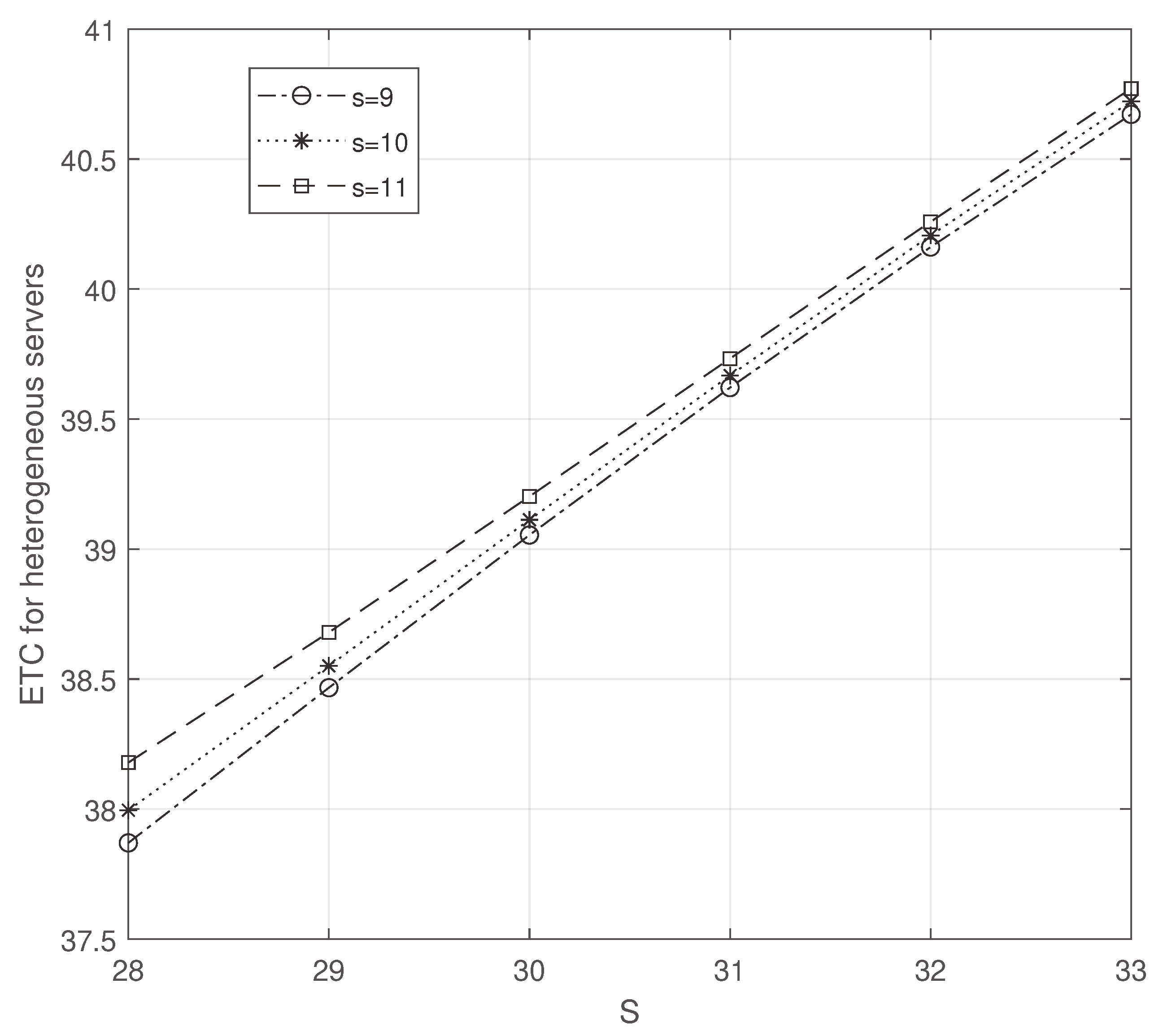
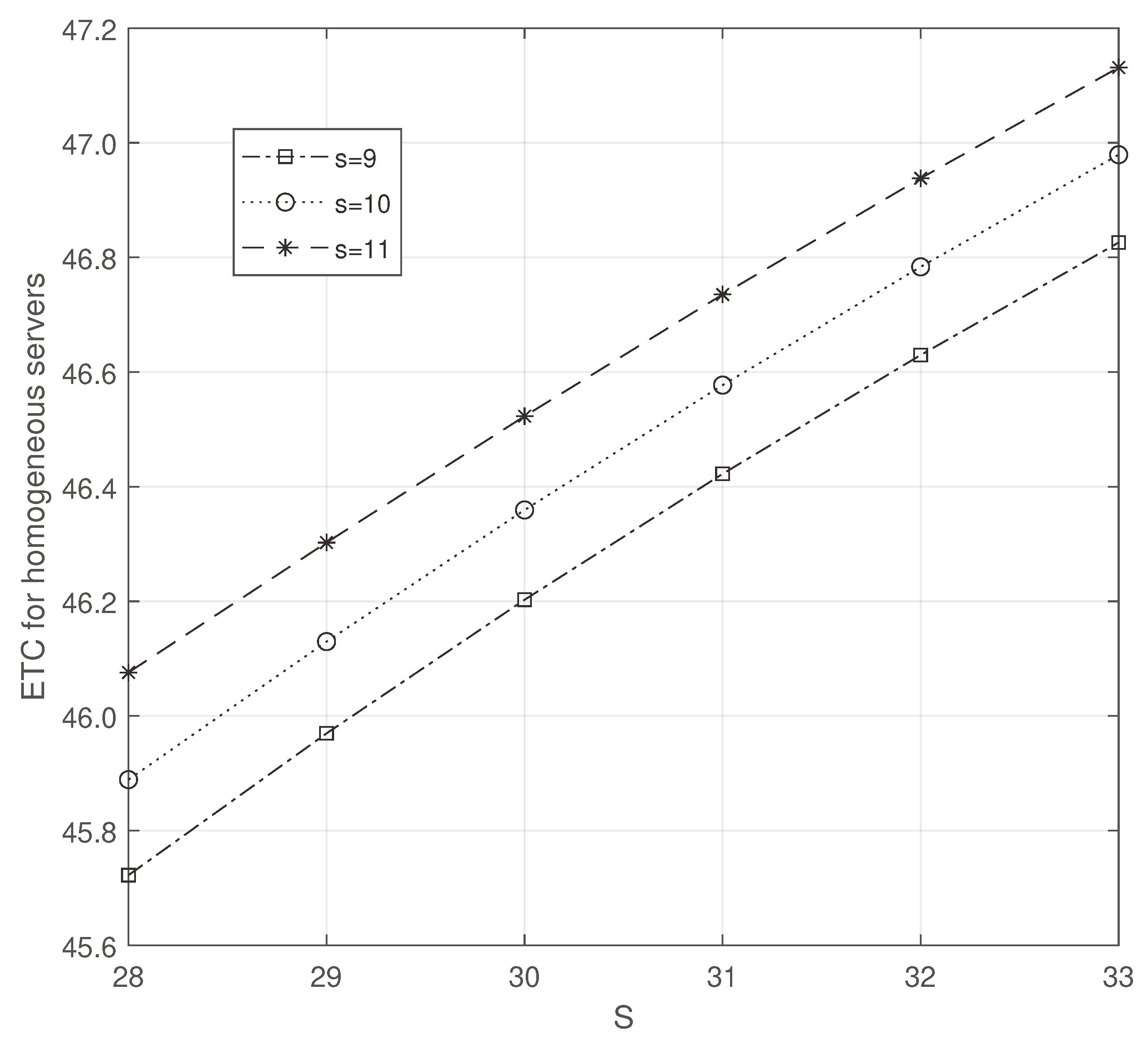
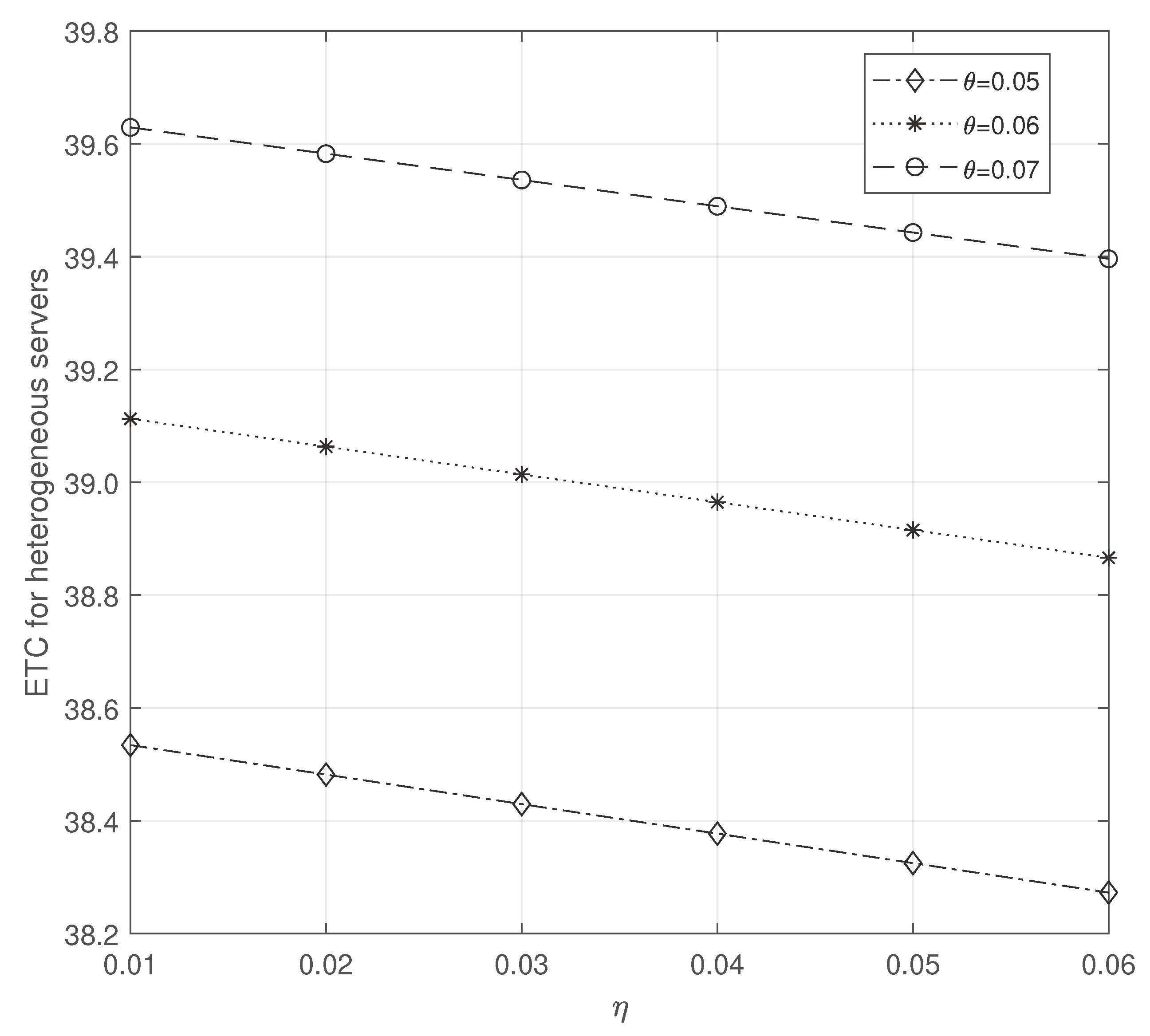
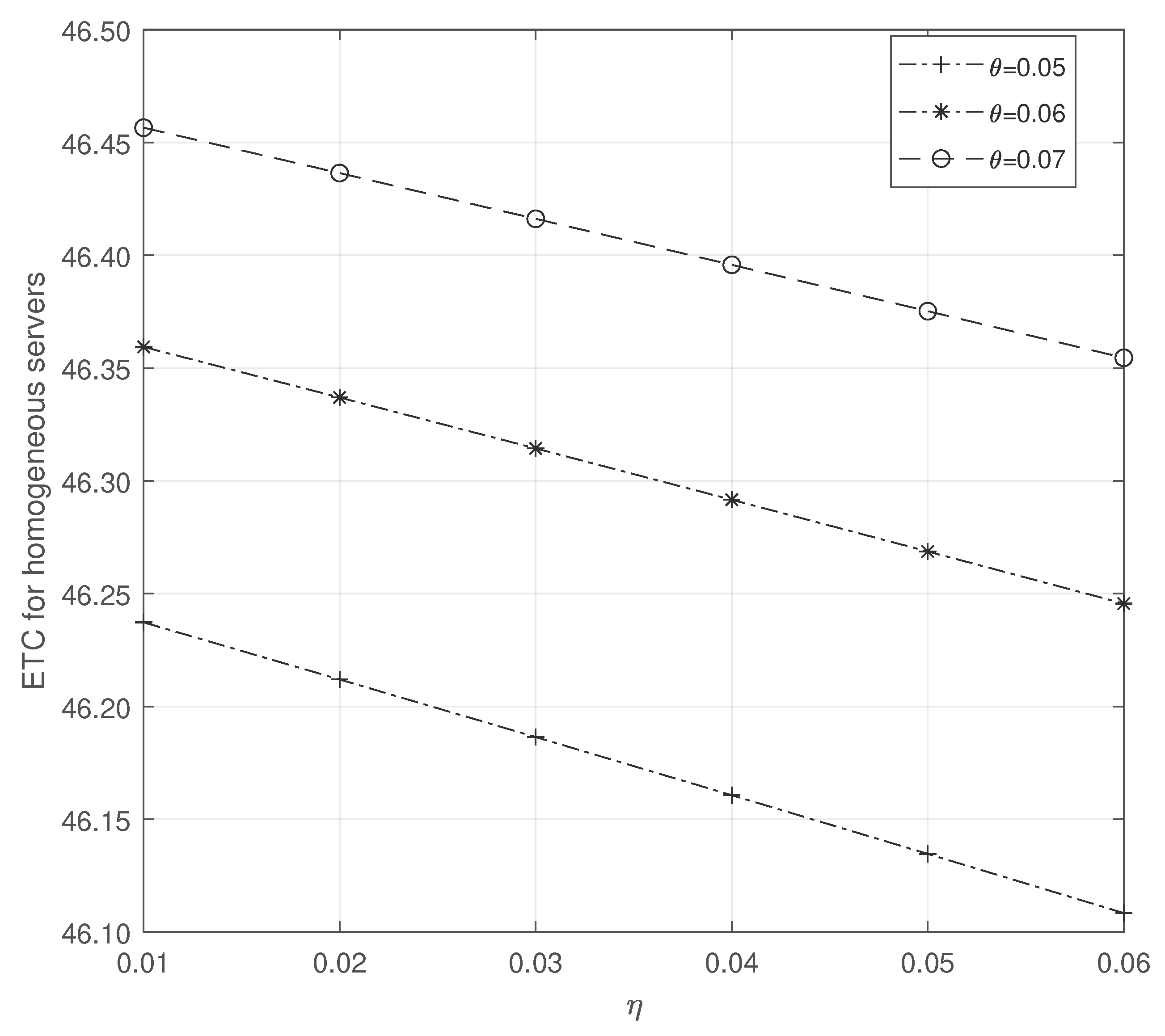
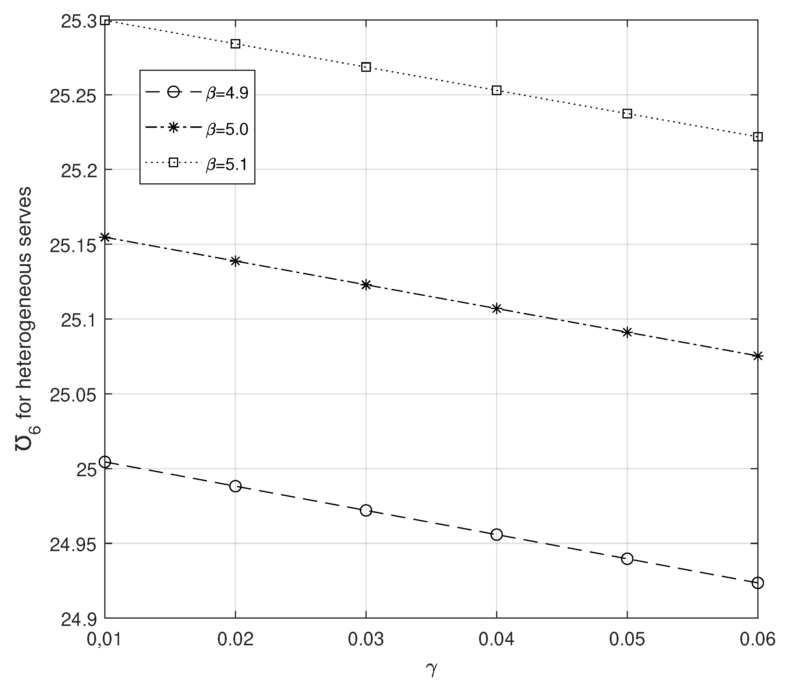
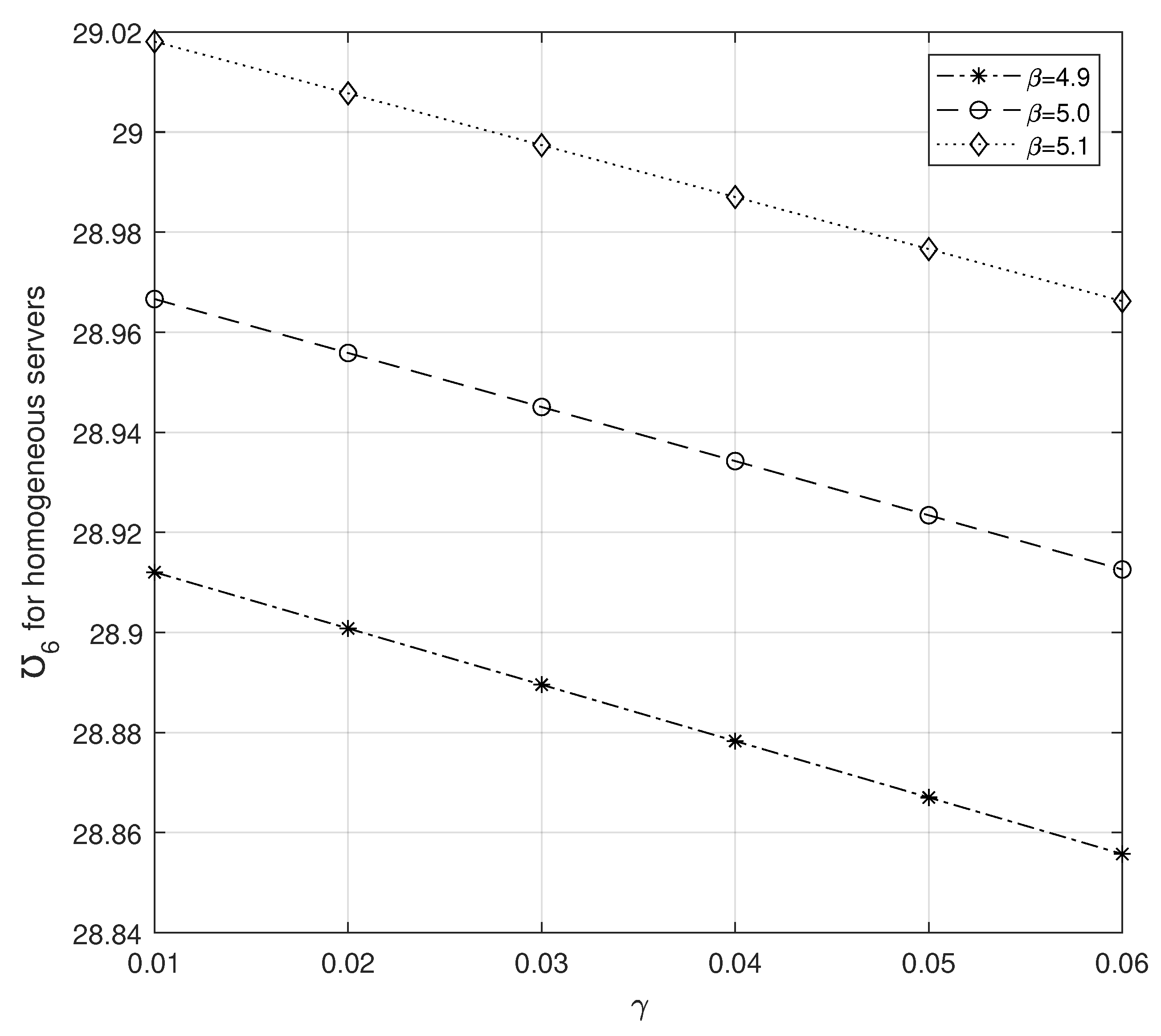
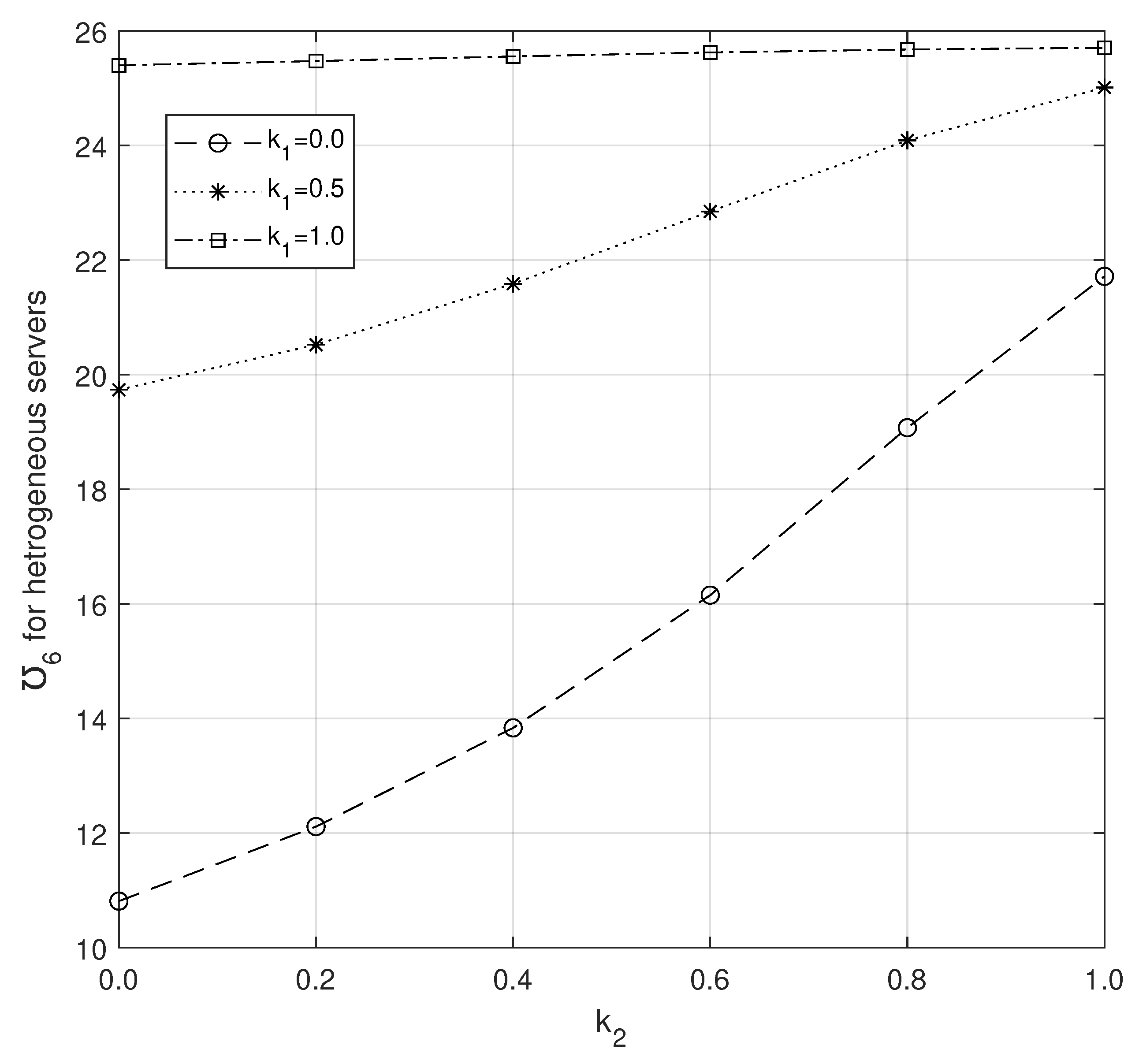
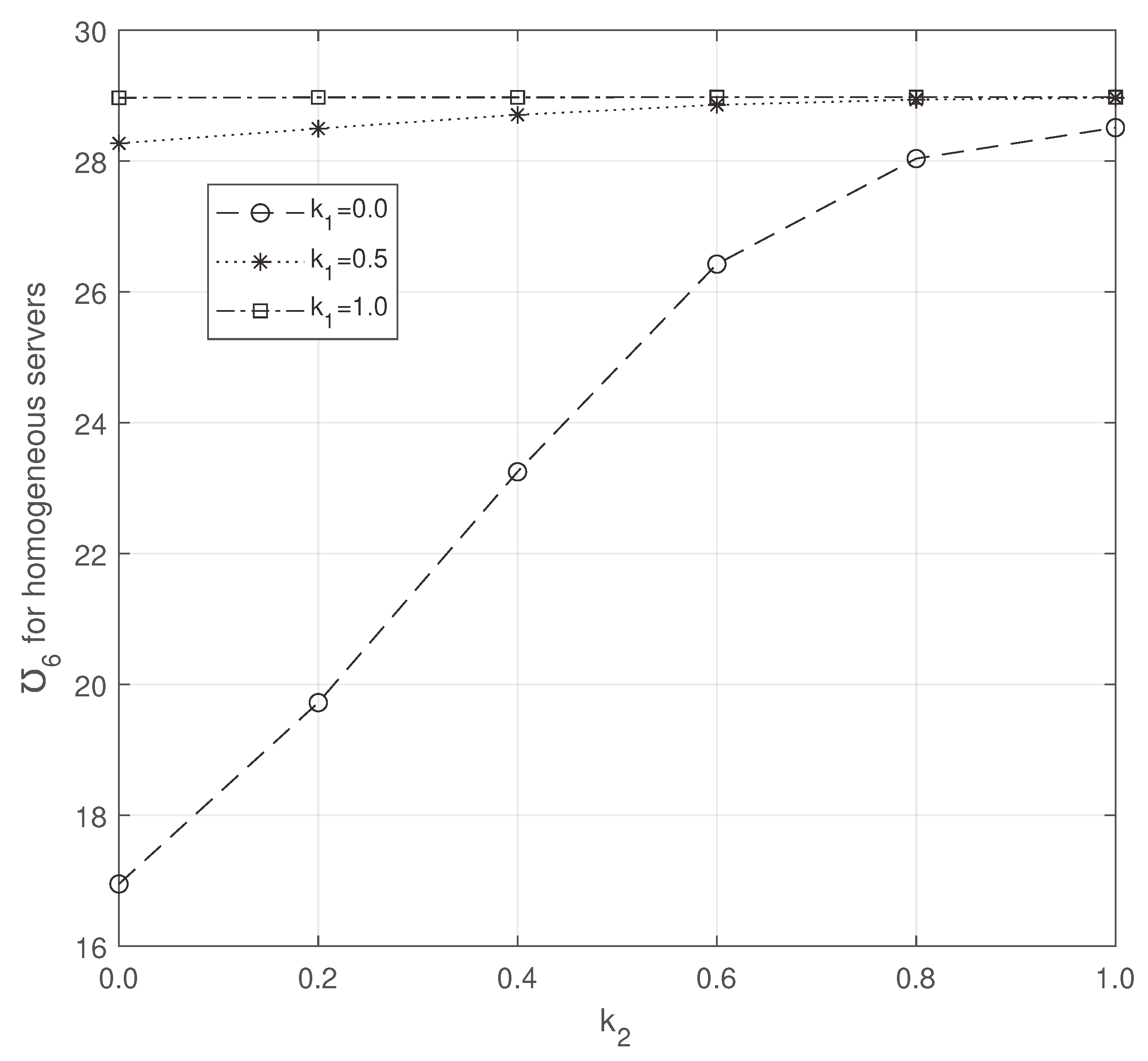
In this section, we compare the efficiency of homogeneous and heterogeneous servers in ETC through
Figure 2,
Figure 3,
Figure 4,
Figure 5,
Figure 6,
Figure 7,
Figure 8,
Figure 9,
Figure 10,
Figure 11,
Figure 12 and
Figure 13.
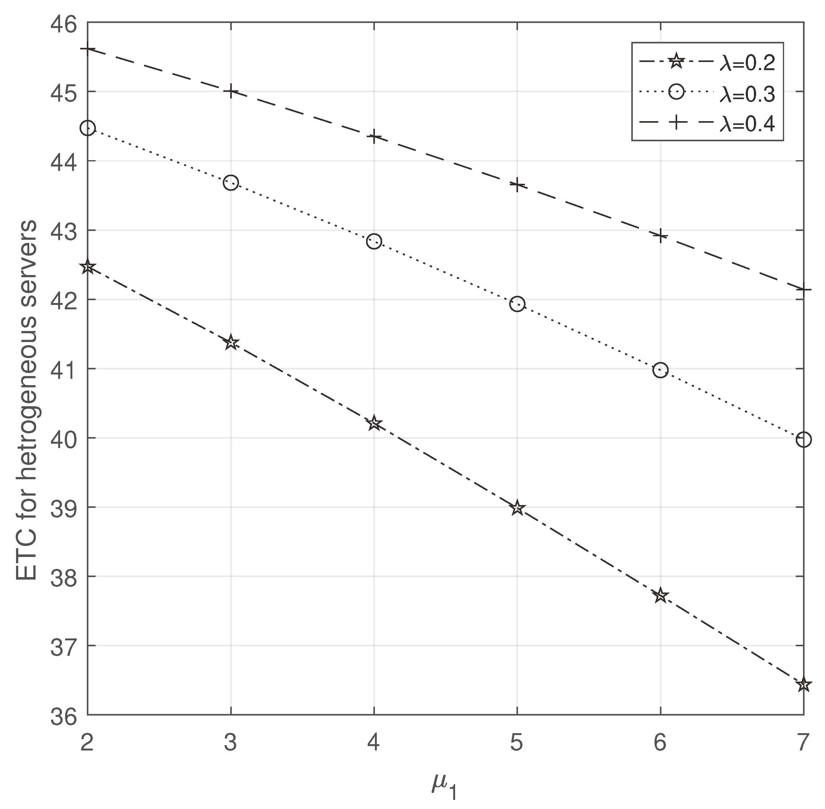
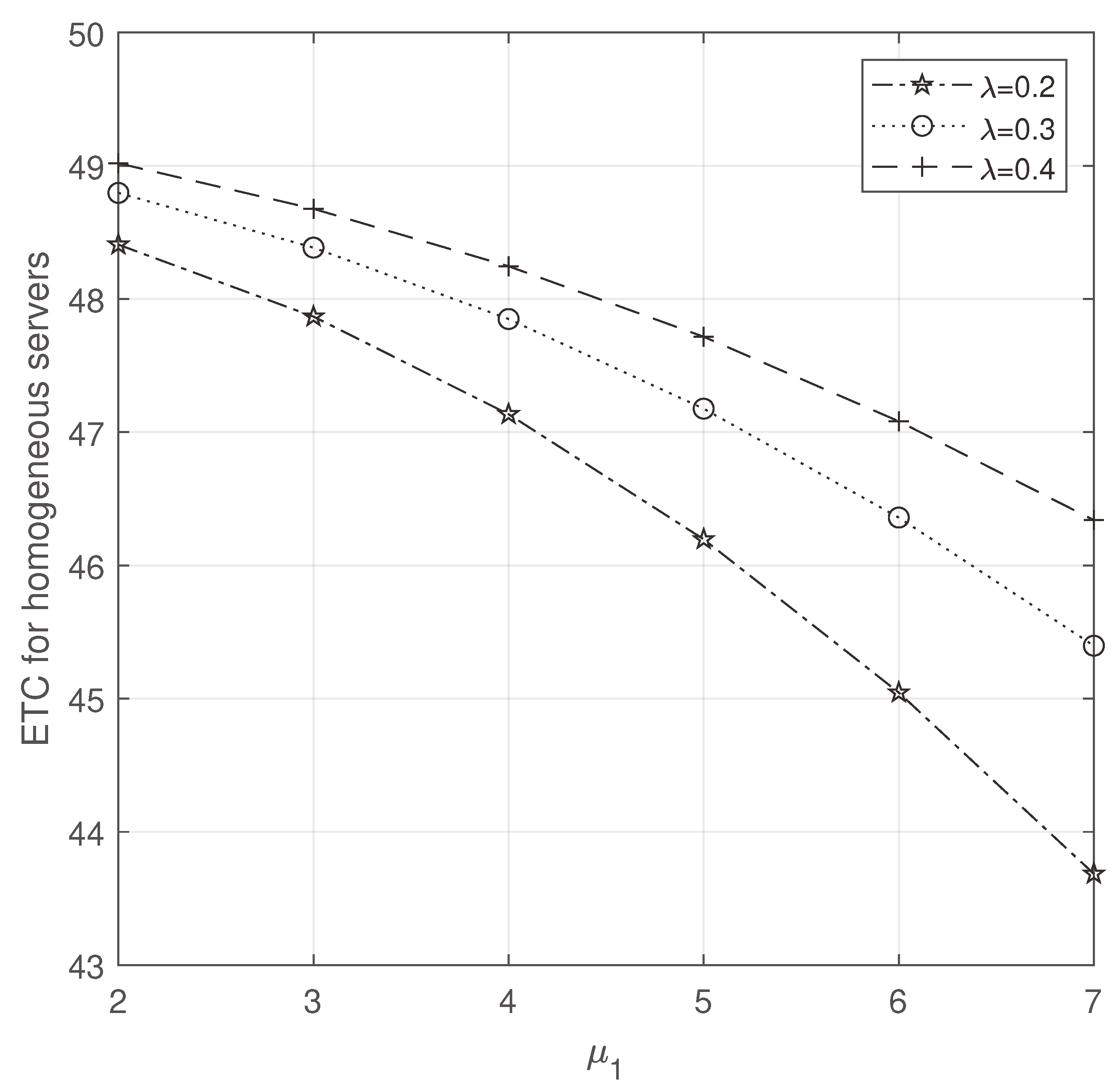
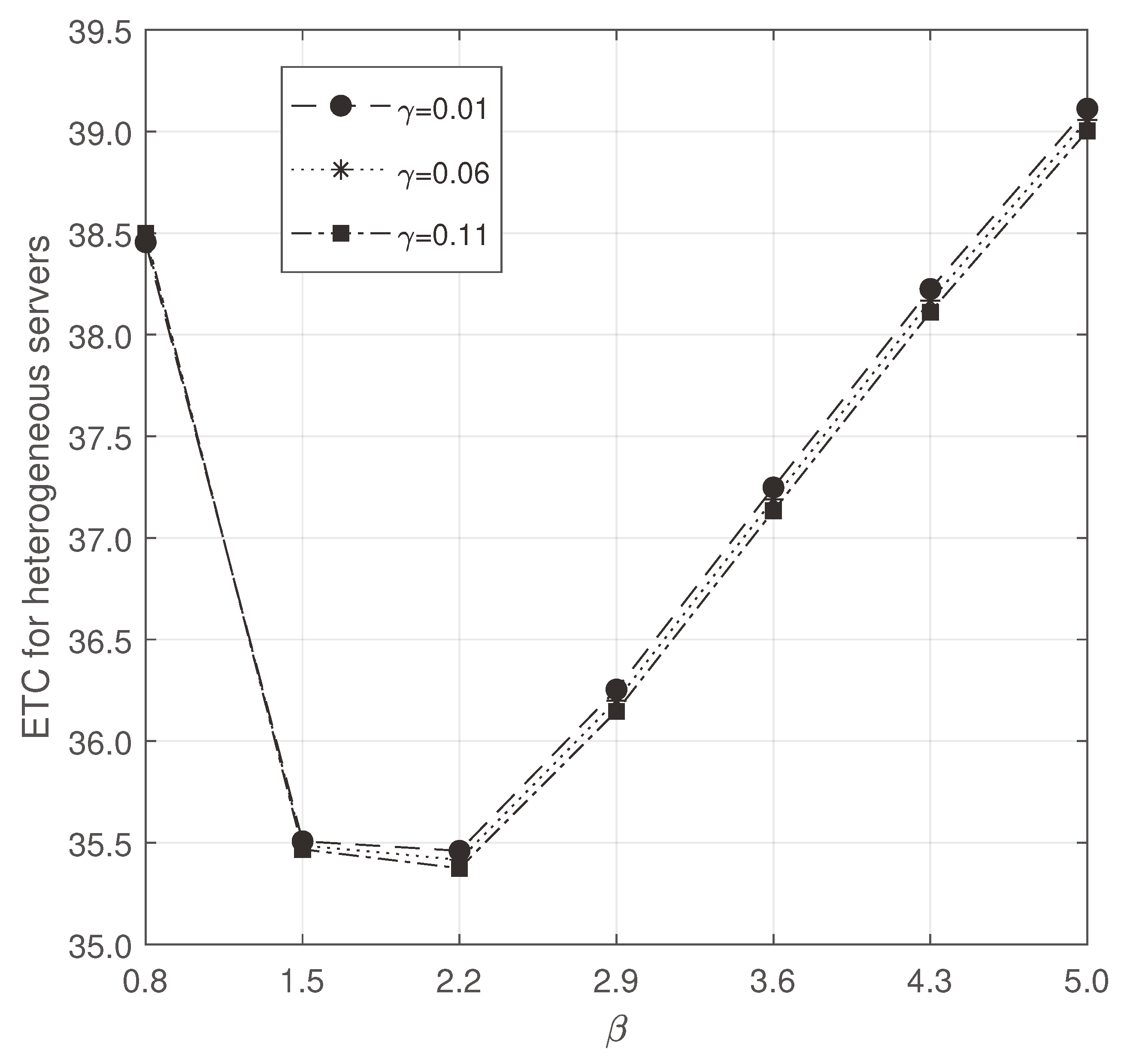
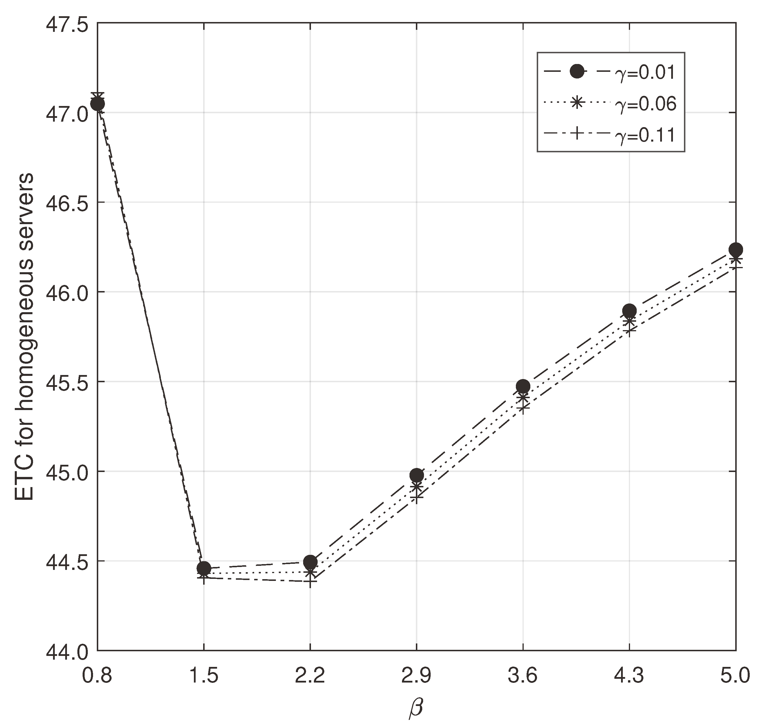
Observing
Figure 2 and
Figure 3, we note that while increasing
and
, ETC increases and decreases, respectively. But compared to homogeneous servers, ETC is more efficient on heterogeneous servers.
While increasing
S and
s, we note that ETC increases in both
Figure 4 and
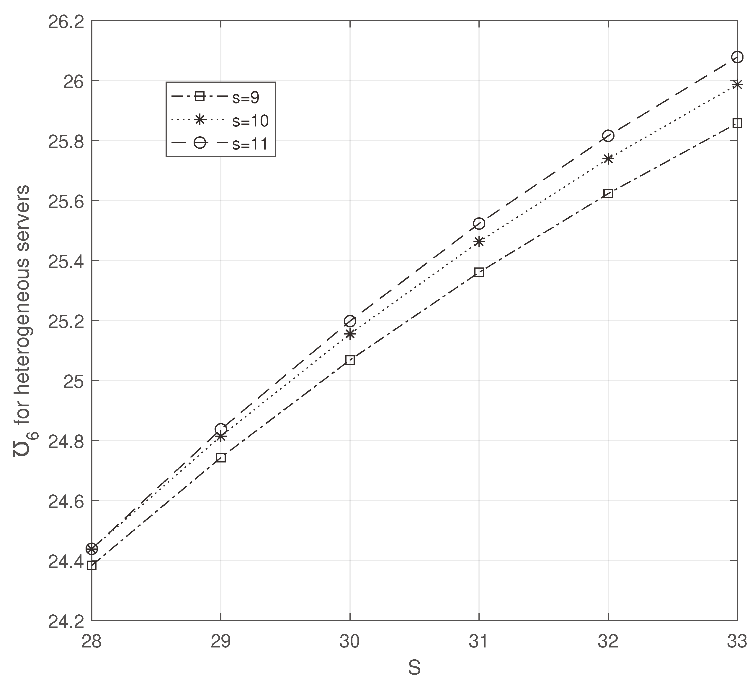
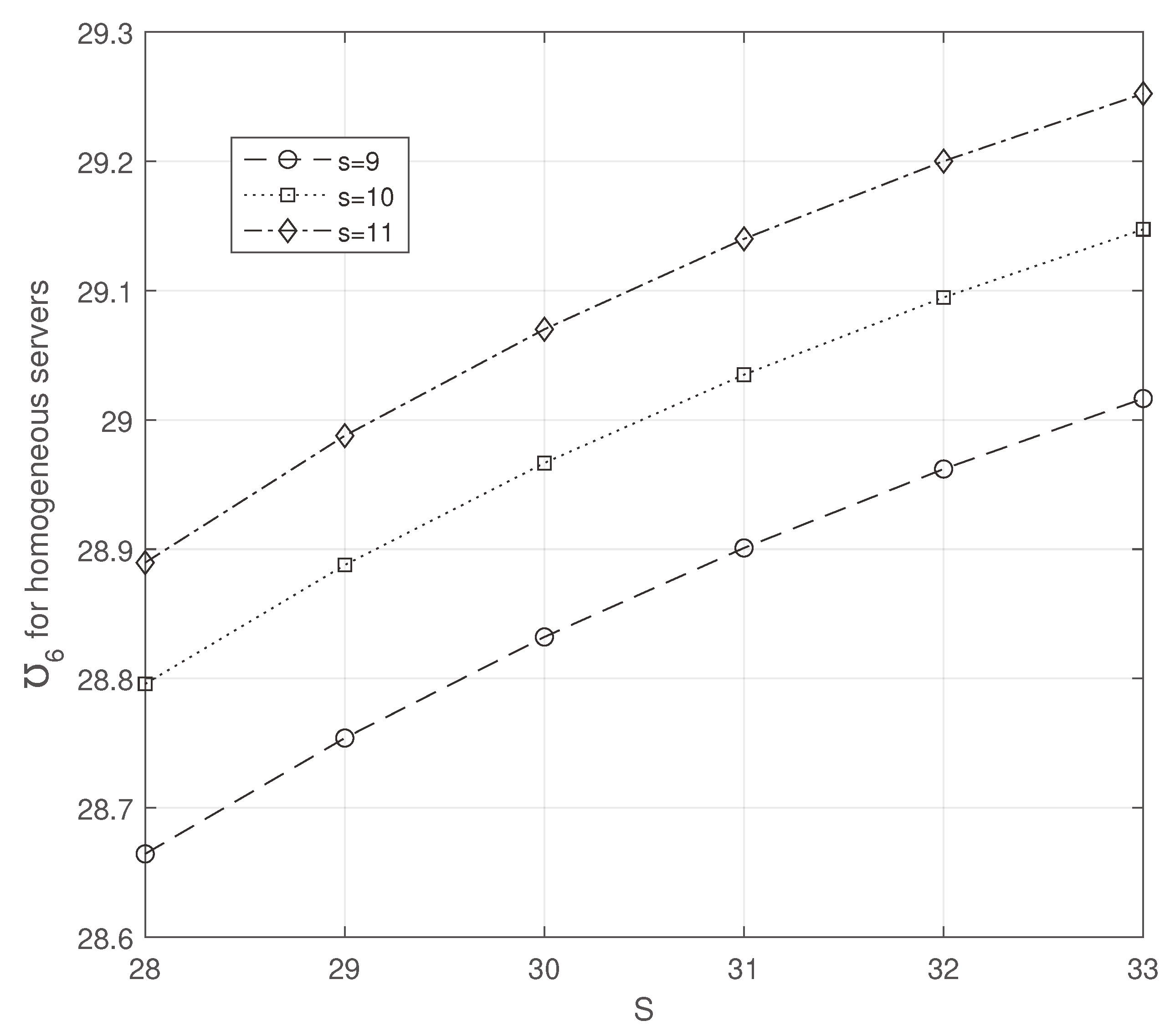
Figure 5. But the value of ETC is minimum in
Figure 4.
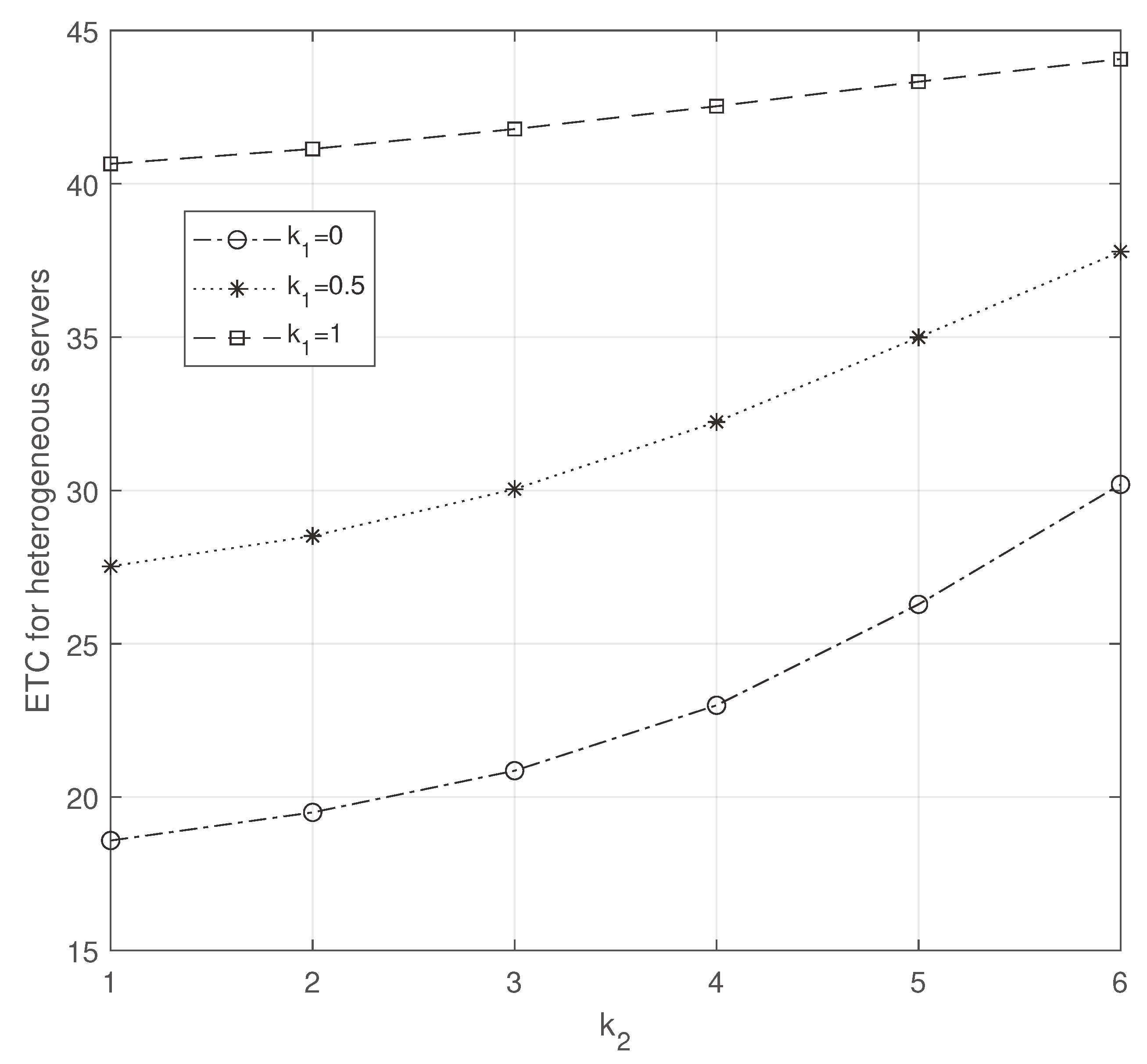
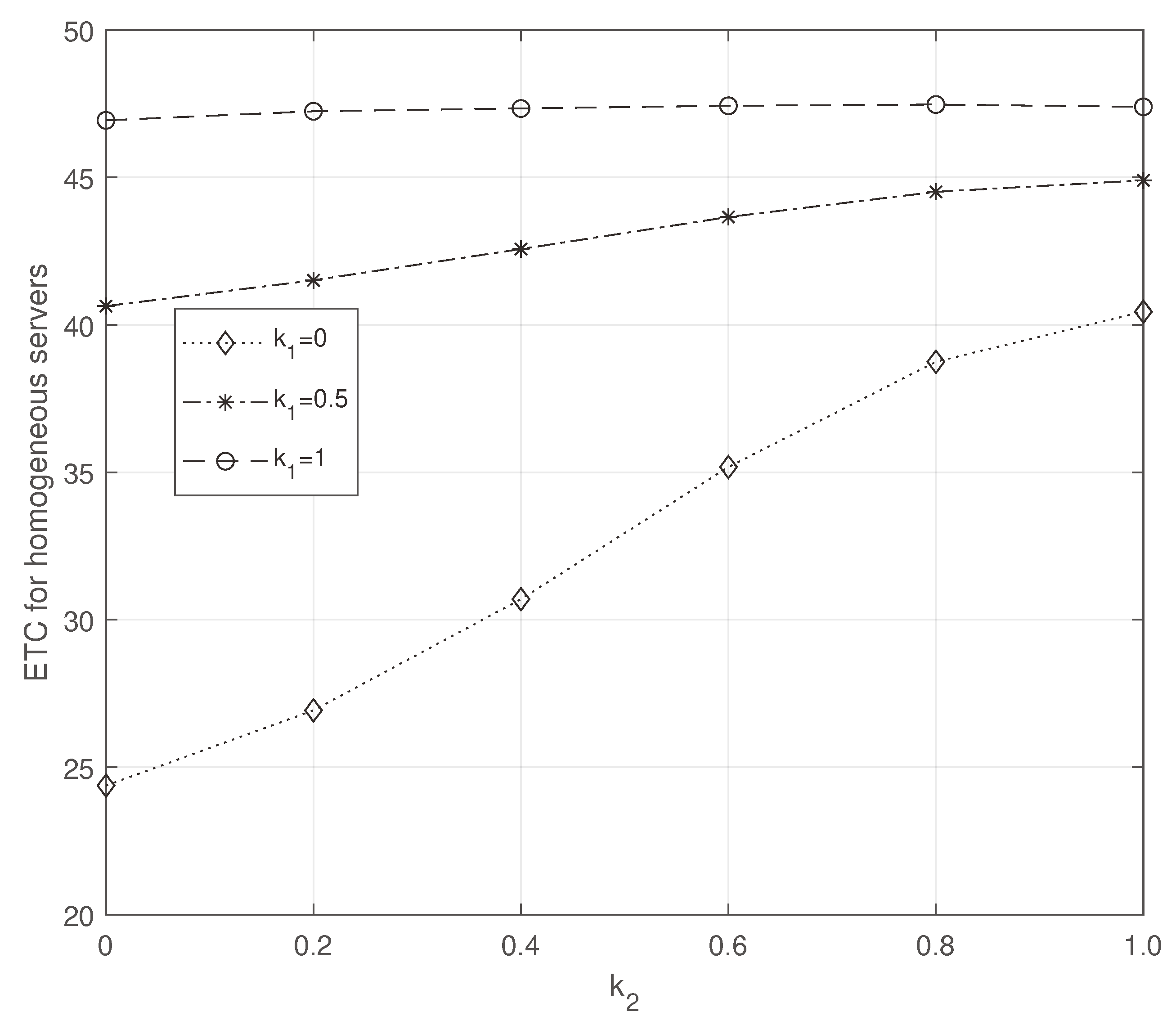
Figure 6 and
Figure 7 show that
increases the ETC while
decreases it. But ultimately, comparing both figures, one can note that ETC is more efficient only in
Figure 6.
Parameters
and
are varied in
Figure 8 and
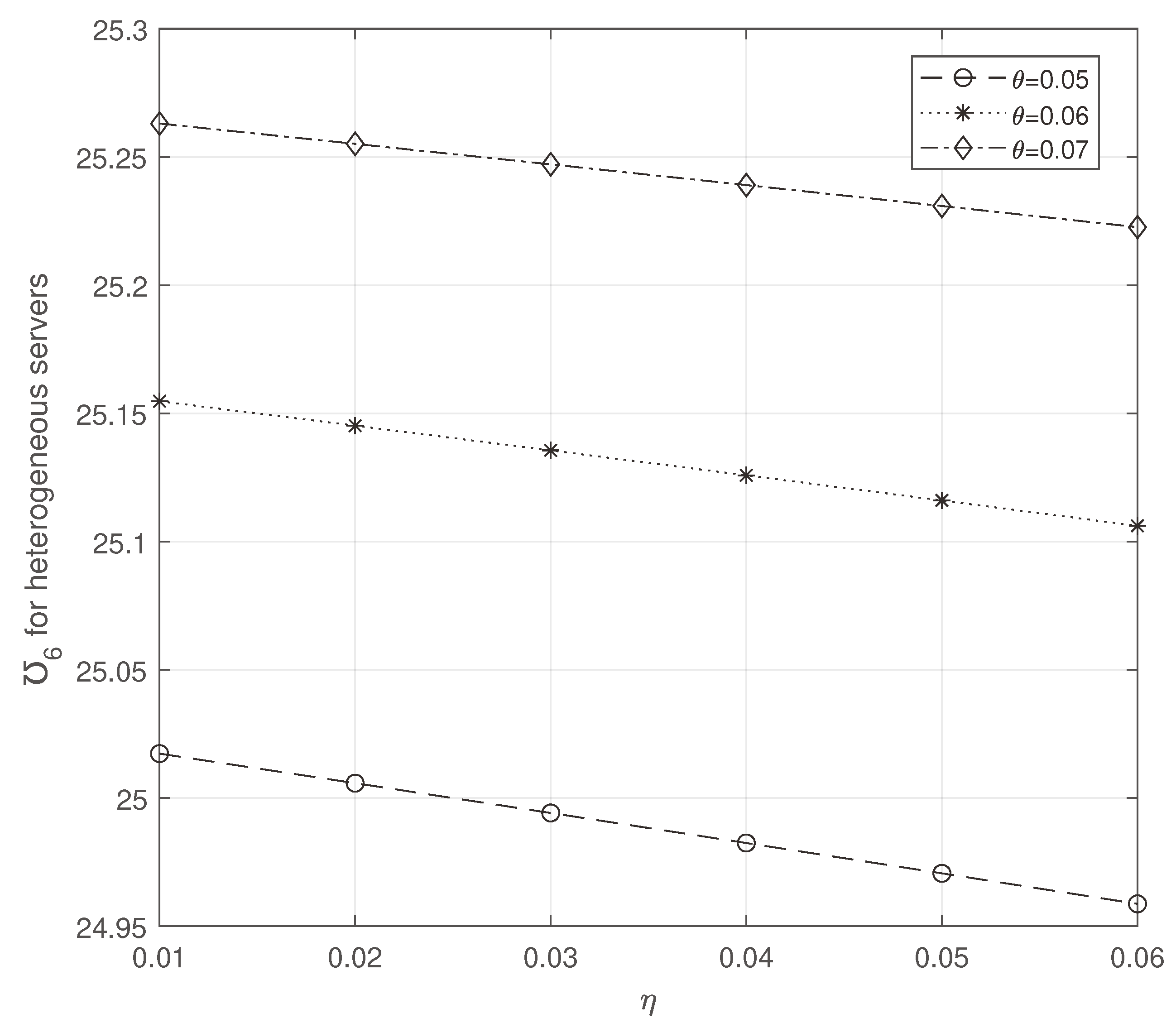
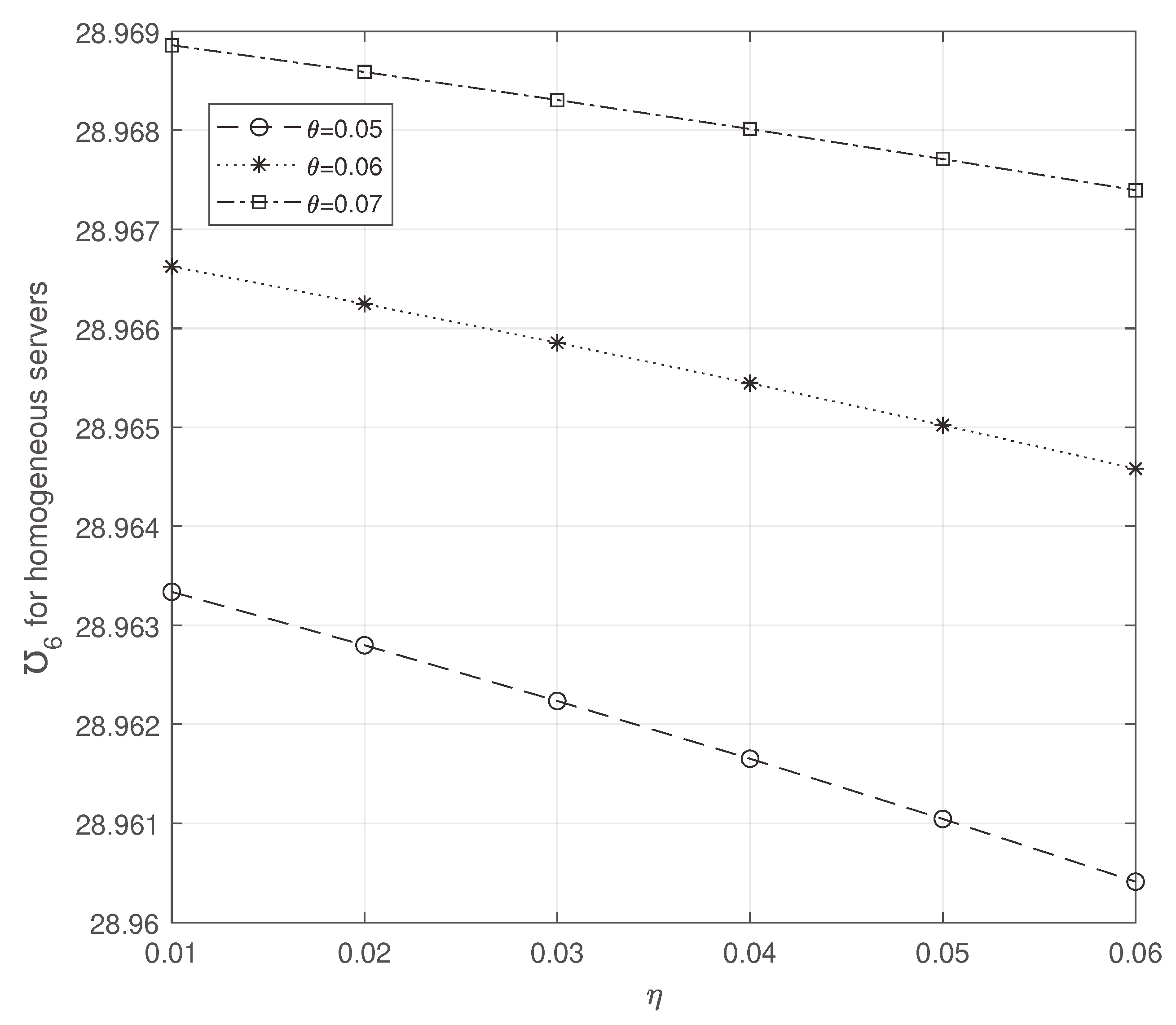
Figure 9. They show us that there exists convexity for both heterogeneous and homogeneous servers while varying
. But the obtained convexity is more efficient for heterogeneous servers. Also, the ETC is decreased while varying
for both homogeneous and heterogeneous servers.
The scaling factors
and
are varied to compare the heterogeneous and homogeneous servers in
Figure 10 and
Figure 11. We note that while increasing the scaling factors, arrival occurs, so ETC increases. Compared to homogeneous servers, heterogeneous servers efficiently optimize the ETC.
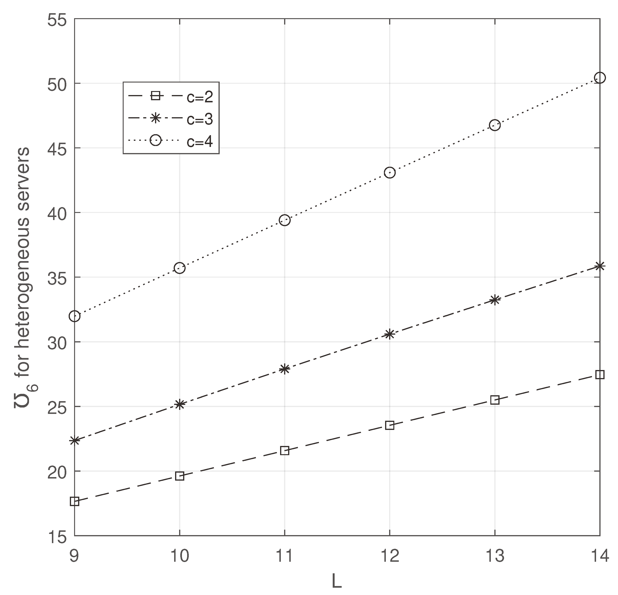
In
Figure 12 and
Figure 13,
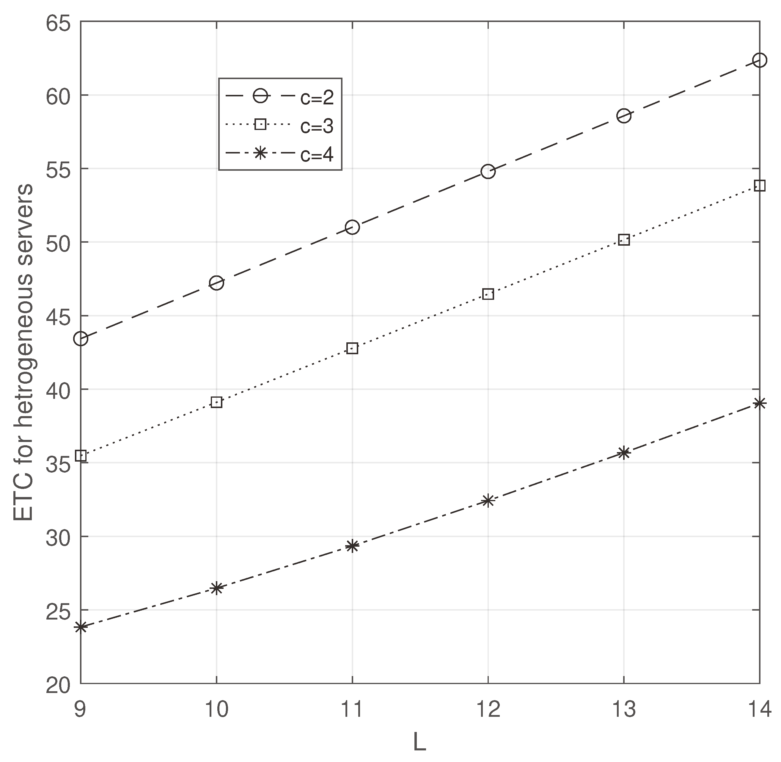
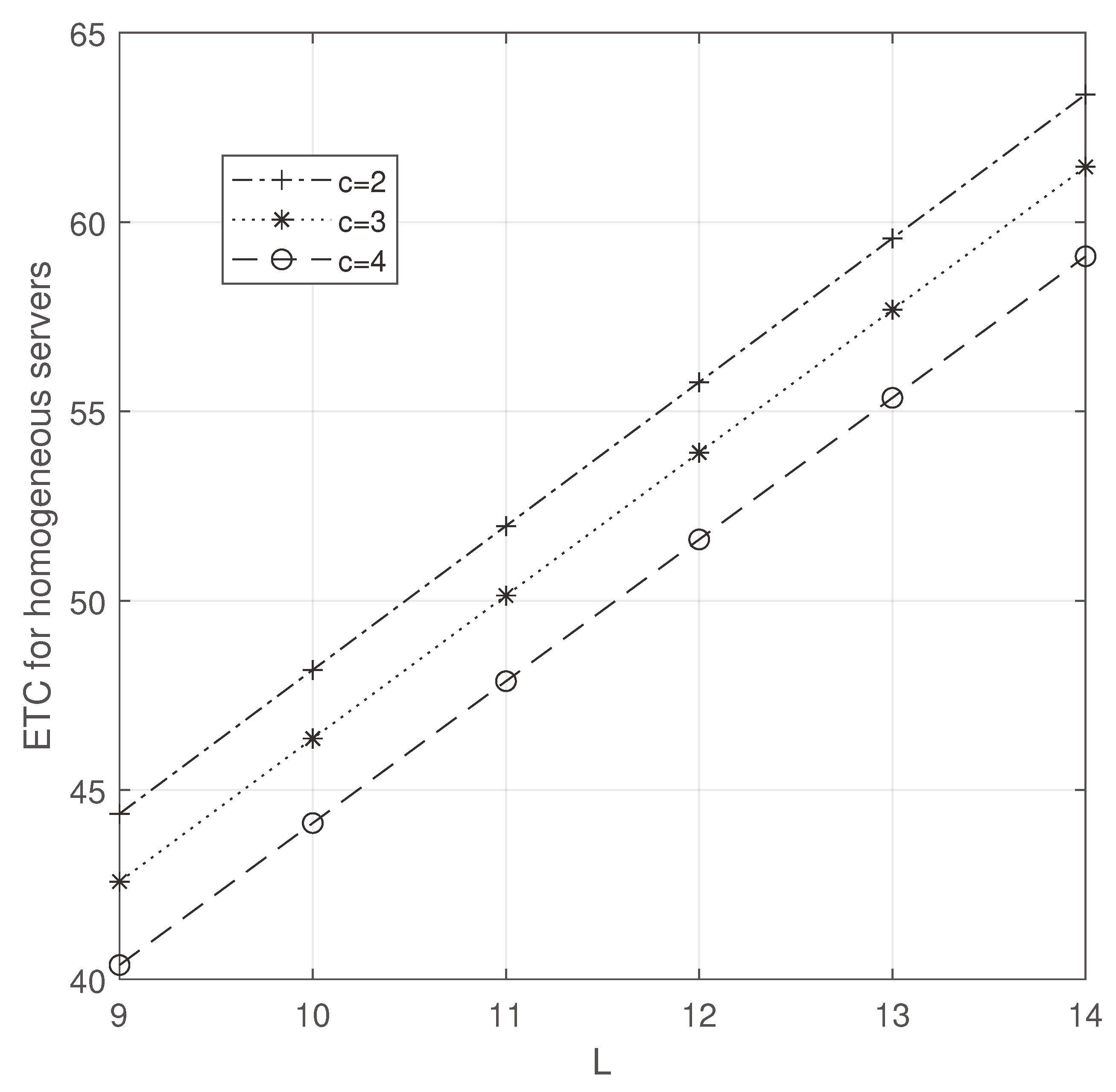
L and
c are varied to see the changes in ETC. While increasing them, ETC increased as we expected. However, ETC is minimum in
Figure 12.
From the above comparative analysis, we witness that heterogeneous servers play a vital role in controlling the efficiency of the ETC.
5.2. A Comparative Analysis of Heterogeneous and Homogeneous Servers in Average Number of Busy Servers
In this section, we compare the heterogeneous and homogeneous servers, analyzing the average number of busy servers from
Figure 14,
Figure 15,
Figure 16,
Figure 17,
Figure 18,
Figure 19,
Figure 20,
Figure 21,
Figure 22,
Figure 23,
Figure 24 and
Figure 25.
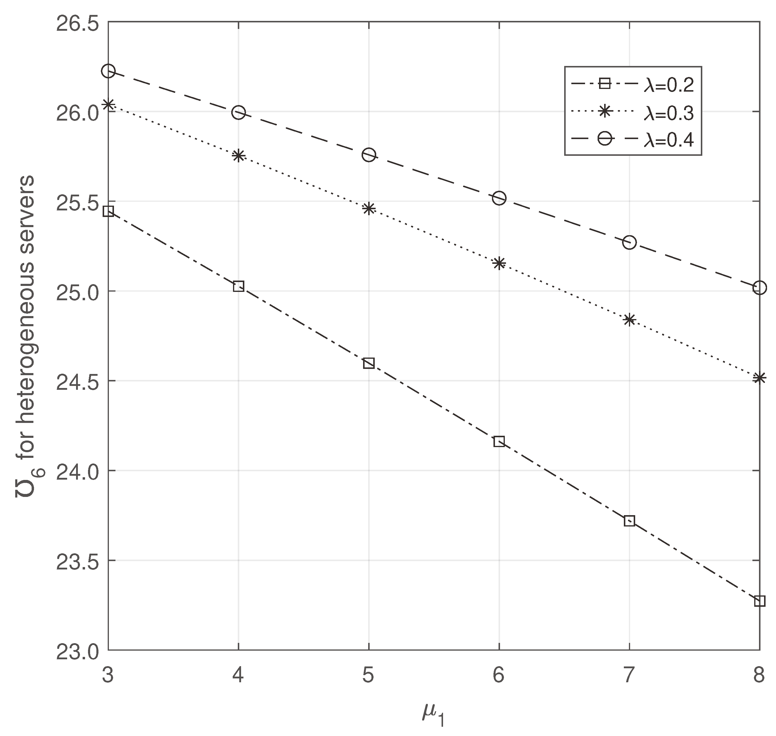
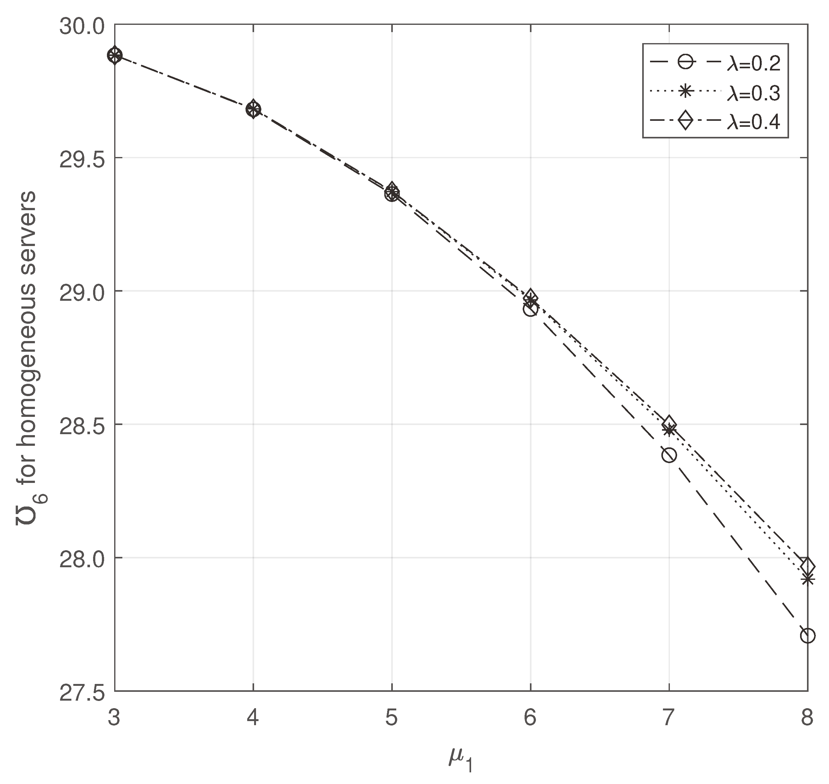
From
Figure 14 and
Figure 15, we note that the average number of customers increases while increasing
and decreases while increasing
. Though there is a change in varying them,
is minimum on heterogeneous servers only.
In
Figure 16 and
Figure 17, inventory capacity and reorder point are varied to discuss the average busy servers. Though
increases while increasing
S and
s, the minimum value is obtained by varying the heterogeneous servers.
Figure 18 and
Figure 19 demonstrate the effect of varying the parameters
and
on
. We notice that
decreases while increasing
, and it increases at the same time while increasing
. Observing both figures, we notice that
Figure 18 is more efficient.
Figure 20 and
Figure 21 show us that
decreases while varying the parameter
and
increases while varying the parameter
. But observing the figures, we clearly notice that heterogeneous servers are minimized.
In
Figure 22 and
Figure 23, the scaling factors for the arrival rate and the retrial rate are varied. As expected,
is increased for
and
in both figures. But
Figure 22 obtained the minimum
than the other one.
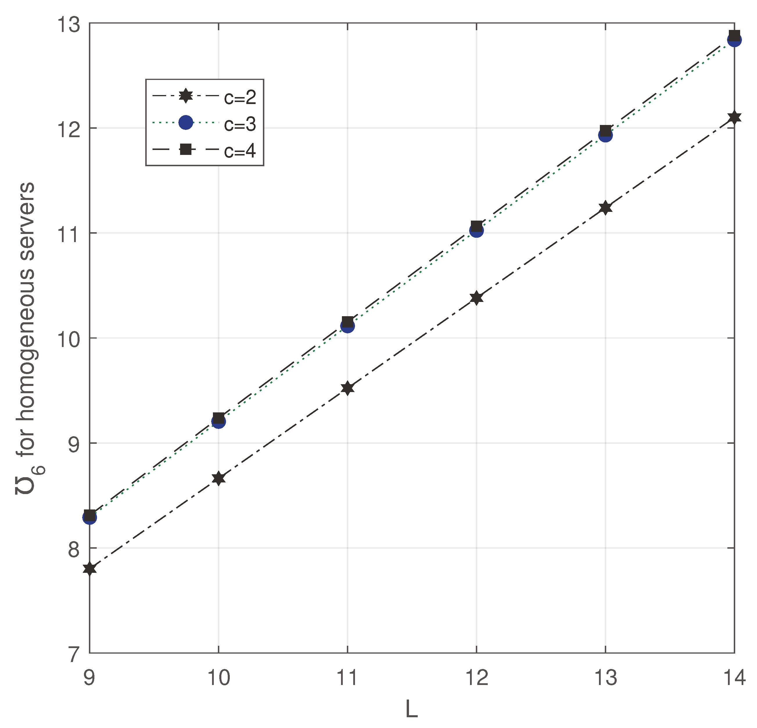
In
Figure 24 and
Figure 25, we have analysed the average number of busy servers under the variation of waiting hall size and number of servers. While increasing both of them, we notice that
is increasing. Though they increase, we could notice that the value of
is minimum in
Figure 24.
The above discussions deal with the comparison of heterogeneous and homogeneous servers on average busy servers. From all the figures, though all the parameters involve their characteristics, the optimized value is obtained for the heterogeneous servers only.
5.3. A Comparative Analysis of Homogeneous and Heterogeneous Servers on Waiting time of Customers in Waiting Hall and Orbit
This section analyses the comparative study of heterogeneous and homogeneous over the average number of customers in the waiting hall and orbit, which are shown in
Table 1,
Table 2,
Table 3,
Table 4,
Table 5,
Table 6 and
Table 7. The characteristics of the parameters are given below.
We notice that increasing the causes an increase in and . This is because of the decrease in the duration of the arrival of primary customers.
While increasing the parameter , we know that a number of customers enter the waiting hall from orbit. That’s why increases and decreases while increasing .
The average service time is usually reduced while increasing the parameter , or the number of servers. So the and decrease if we increase the values of and c.
The perishable time decreases if the rate increases. So the average customers’ level in the orbit and waiting hall increases while varying the parameter .
When we increase the rate of , the lead time of replenishment decreases in nature. So the customers from the orbit and waiting hall need not wait too long in the stock-out time. So and decrease while varying .
The characteristics of parameters remain the same in
Table 1,
Table 2,
Table 3,
Table 4,
Table 5,
Table 6 and
Table 7. Also, we witness that the minimum values of
and
are obtained on heterogeneous servers. This shows us that the role of heterogeneous servers is inevitable in reducing the waiting time of customers, as waiting time and the mean number of customers are directly proportional to each other.
5.4. A Comparative Analysis of Heterogeneous and Homogeneous Servers in Fraction of Successful Retrial Rate
In this section, a heterogeneous vs. homogeneous server comparison is done over a fraction of the successful retrial rate, which is given in
Table 9 and
Table 11. The characteristics of each parameter are explained below.
While increasing the arrival rates of and , the waiting hall becomes full more often, which usually decreases the fraction of successful retrials.
If we increase the rate of , the customer’s impatient rate increases. But the orbital customers soon occupy the waiting hall, and it becomes full at some time. So it decreases the fraction of successful retrials.
Similarly, when we increase the rate of , it decreases the . Because it boosts the perishability of items in the inventory.
If the service time or number of servers is increased, the customer waiting time directly decreases. So while increasing and c causes a decrease in
Increasing the rate ensures the availability and on-time replenishment of stock. So increases while we increase the parameter
Based on the observation, we note that in
Table 9, the obtained value is much minimum than in
Table 11. This shows us that heterogeneous servers are more optimized than homogeneous servers.
5.5. A Comparative Analysis of Homogeneous and Heterogeneous Servers in Average Impatient Rate
Table 13 and
Table 15 analysed the expected impatient rate on heterogeneous servers and homogeneous servers. Each parameter’s discussions are given below.
Increasing the waiting hall size and the arrival rate causes an increase in . So the average impatience rate for a customer increases.
When we vary the value of , decreases but increases along with it. So the average impatience rate for a customer increases.
Similarly, while increasing the value of scaling factors for retrial and arrival rate, they increase the expected impatient rate for a customer.
If we increase the rate of , impatient time decreases. So a customer’s expected impatient rate increases in nature.
Similarly, increasing the perishable rate leads to a decrease in the .
Unlike the other parameters, and c decrease while increasing them. Because, they decrease the average waiting time of customers in the waiting hall.
Similarly, average lead time decreases while we increase the rate value . So the average impatient rate decreases while increasing
Though the parameters imply their characters independently, from
Table 13 and
Table 15, we can clearly note that the impatient rate is minimal with heterogeneous servers. This shows how heterogeneous servers are more efficient in a multi-server queueing-inventory system to decrease the impatient rate.
5.6. Observations
In each comparison of heterogeneous and homogeneous servers, heterogeneous servers performs efficiently.
Optimal reorder rate for ETC exists for homogeneous and heterogeneous servers.
The arrival rate of customers is influenced by the stock level. Consequently, the average number of busy servers increases.
The FSR increases as the value of c varies, and drops when the value of varies.
The service rate inversely affects the average impatient rate and ETC.
Raising the value of L leads to an increase in the ETC and a rise in the average impatience rate.
Modifying the service rate and adding more servers have a significant impact on the system’s performance.
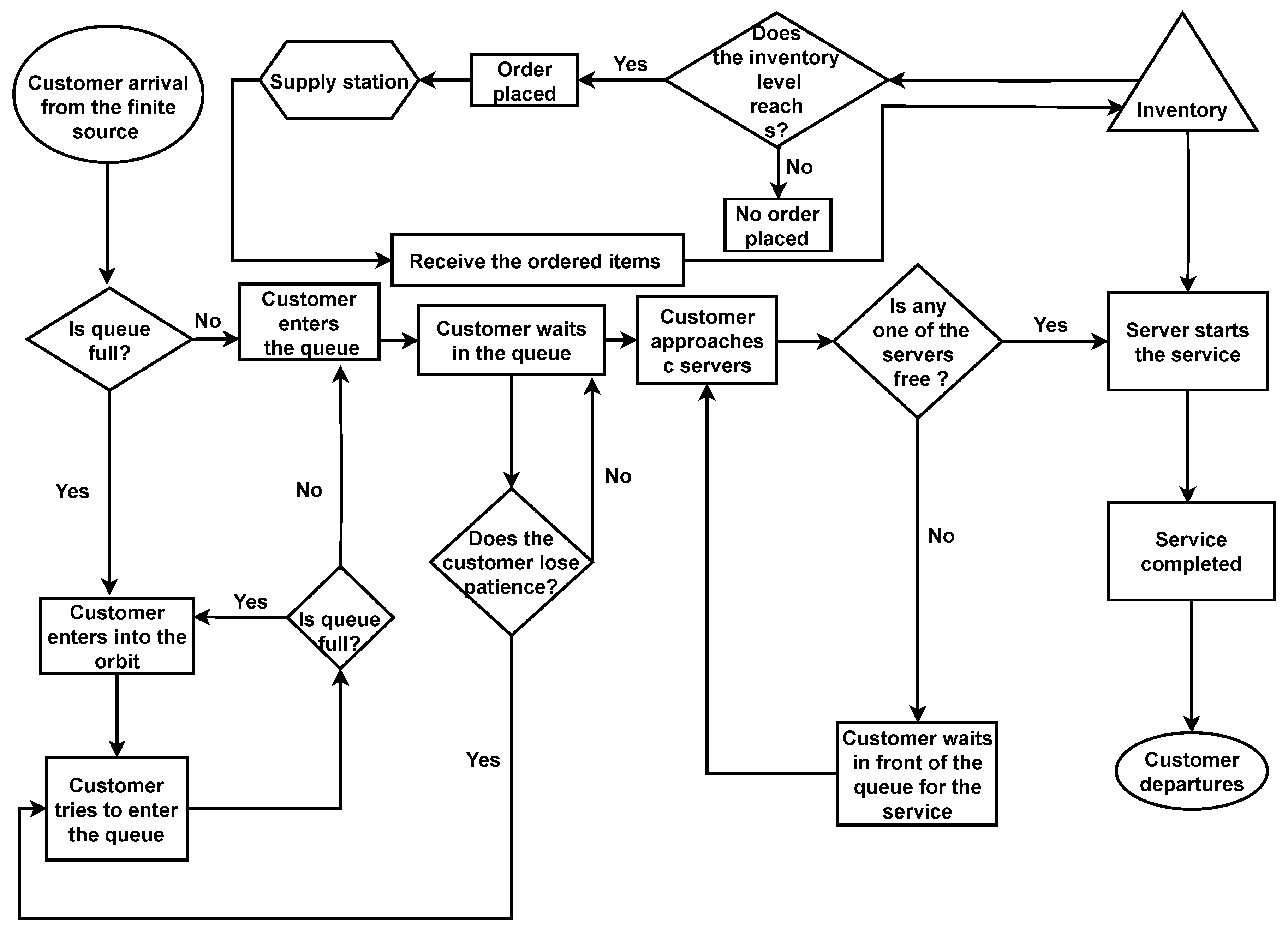
Figure 1.
Flow chart of the model.
Figure 1.
Flow chart of the model.
Figure 2.
ETC for heterogeneous servers: vs .
Figure 2.
ETC for heterogeneous servers: vs .
Figure 3.
ETC for homogeneous servers: vs .
Figure 3.
ETC for homogeneous servers: vs .
Figure 4.
ETC for heterogeneous servers: S vs s.
Figure 4.
ETC for heterogeneous servers: S vs s.
Figure 5.
ETC for homogeneous servers: S vs s.
Figure 5.
ETC for homogeneous servers: S vs s.
Figure 6.
ETC for heterogeneous servers: vs
Figure 6.
ETC for heterogeneous servers: vs
Figure 7.
ETC for homogeneous servers: vs .
Figure 7.
ETC for homogeneous servers: vs .
Figure 8.
ETC for heterogeneous servers: vs .
Figure 8.
ETC for heterogeneous servers: vs .
Figure 9.
ETC for homogeneous servers: vs .
Figure 9.
ETC for homogeneous servers: vs .
Figure 10.
ETC for heterogeneous servers: vs .
Figure 10.
ETC for heterogeneous servers: vs .
Figure 11.
ETC for homogeneous servers: vs .
Figure 11.
ETC for homogeneous servers: vs .
Figure 12.
ETC for heterogeneous servers: c vs L.
Figure 12.
ETC for heterogeneous servers: c vs L.
Figure 13.
ETC for homogeneous servers: c vs L.
Figure 13.
ETC for homogeneous servers: c vs L.
Figure 14.
Average number of heterogeneous busy servers: vs .
Figure 14.
Average number of heterogeneous busy servers: vs .
Figure 15.
Average number of homogeneous busy servers: vs .
Figure 15.
Average number of homogeneous busy servers: vs .
Figure 16.
Average number of heterogeneous busy servers: S vs s.
Figure 16.
Average number of heterogeneous busy servers: S vs s.
Figure 17.
Average number of homogeneous busy servers: S vs s.
Figure 17.
Average number of homogeneous busy servers: S vs s.
Figure 18.
Average number of heterogeneous busy servers: vs .
Figure 18.
Average number of heterogeneous busy servers: vs .
Figure 19.
Average number of homogeneous busy servers: vs .
Figure 19.
Average number of homogeneous busy servers: vs .
Figure 20.
Average number of heterogeneous busy servers: vs .
Figure 20.
Average number of heterogeneous busy servers: vs .
Figure 21.
Average number of homogeneous busy servers: vs .
Figure 21.
Average number of homogeneous busy servers: vs .
Figure 22.
Average number of heterogeneous busy servers: vs .
Figure 22.
Average number of heterogeneous busy servers: vs .
Figure 23.
Average number of homogeneous busy servers: vs
Figure 23.
Average number of homogeneous busy servers: vs
Figure 24.
Average number of heterogeneous busy servers: c vs L.
Figure 24.
Average number of heterogeneous busy servers: c vs L.
Figure 25.
Average number of homogeneous busy servers: c vs L.
Figure 25.
Average number of homogeneous busy servers: c vs L.
Table 1.
Average number of customers in the waiting hall for heterogeneous servers.
Table 1.
Average number of customers in the waiting hall for heterogeneous servers.
| c |
|
|
|
|
0.2 |
0.3 |
0.4 |
| |
|
|
|
|
5.0 |
6.0 |
7.0 |
5.0 |
6.0 |
7.0 |
5.0 |
6.0 |
7.0 |
| 2 |
4 |
0.05 |
0.01 |
9.29024 |
9.20647 |
9.11723 |
9.50086 |
9.44260 |
9.38050 |
9.61429 |
9.56976 |
9.52228 |
| |
|
|
0.02 |
9.29258 |
9.20896 |
9.11987 |
9.50272 |
9.44460 |
9.38263 |
9.61581 |
9.57139 |
9.52403 |
| |
|
|
0.03 |
9.29493 |
9.21147 |
9.12253 |
9.50459 |
9.44661 |
9.38478 |
9.61733 |
9.57304 |
9.52579 |
| |
|
0.06 |
0.01 |
9.34397 |
9.26664 |
9.18416 |
9.53357 |
9.47938 |
9.42159 |
9.63660 |
9.59493 |
9.55050 |
| |
|
|
0.02 |
9.34614 |
9.26896 |
9.18663 |
9.53529 |
9.48124 |
9.42358 |
9.63800 |
9.59645 |
9.55213 |
| |
|
|
0.03 |
9.34833 |
9.27130 |
9.18912 |
9.53703 |
9.48310 |
9.42557 |
9.63942 |
9.59798 |
9.55377 |
| |
|
0.07 |
0.01 |
9.38950 |
9.31773 |
9.24115 |
9.56178 |
9.51114 |
9.45712 |
9.65614 |
9.61700 |
9.57525 |
| |
|
|
0.02 |
9.39152 |
9.31990 |
9.24346 |
9.56339 |
9.51287 |
9.45897 |
9.65746 |
9.61841 |
9.57677 |
| |
|
|
0.03 |
9.39356 |
9.32209 |
9.24578 |
9.56500 |
9.51461 |
9.46084 |
9.65877 |
9.61984 |
9.57830 |
| |
5 |
0.05 |
0.01 |
9.22496 |
9.12961 |
9.02785 |
9.45445 |
9.38815 |
9.31743 |
9.57789 |
9.52710 |
9.47293 |
| |
|
|
0.02 |
9.22778 |
9.13261 |
9.03103 |
9.45667 |
9.39052 |
9.31995 |
9.57969 |
9.52904 |
9.47500 |
| |
|
|
0.03 |
9.23062 |
9.13563 |
9.03424 |
9.45890 |
9.39291 |
9.32249 |
9.58150 |
9.53098 |
9.47707 |
| |
|
0.06 |
0.01 |
9.28575 |
9.19801 |
9.10428 |
9.49192 |
9.43045 |
9.36484 |
9.60376 |
9.55640 |
9.50587 |
| |
|
|
0.02 |
9.28836 |
9.20079 |
9.10723 |
9.49396 |
9.43265 |
9.36718 |
9.60542 |
9.55819 |
9.50778 |
| |
|
|
0.03 |
9.29099 |
9.20359 |
9.11020 |
9.49602 |
9.43485 |
9.36954 |
9.60709 |
9.55999 |
9.50971 |
| |
|
0.07 |
0.01 |
9.33712 |
9.25593 |
9.16913 |
9.52414 |
9.46687 |
9.40571 |
9.62635 |
9.58200 |
9.53467 |
| |
|
|
0.02 |
9.33953 |
9.25851 |
9.17188 |
9.52603 |
9.46891 |
9.40789 |
9.62789 |
9.58366 |
9.53644 |
| |
|
|
0.03 |
9.34197 |
9.26111 |
9.17464 |
9.52794 |
9.47096 |
9.41007 |
9.62944 |
9.58533 |
9.53823 |
| |
6 |
0.05 |
0.01 |
9.12891 |
9.01788 |
8.89956 |
9.38644 |
9.30929 |
9.22719 |
9.52472 |
9.46547 |
9.40242 |
| |
|
|
0.02 |
9.13235 |
9.02152 |
8.90338 |
9.38910 |
9.31212 |
9.23017 |
9.52687 |
9.46776 |
9.40485 |
| |
|
|
0.03 |
9.13581 |
9.02518 |
8.90723 |
9.39178 |
9.31497 |
9.23318 |
9.52903 |
9.47007 |
9.40729 |
| |
|
0.06 |
0.01 |
9.20075 |
9.09898 |
8.99041 |
9.43147 |
9.36022 |
9.28433 |
9.55634 |
9.50133 |
9.44275 |
| |
|
|
0.02 |
9.20390 |
9.10232 |
8.99393 |
9.43390 |
9.36282 |
9.28708 |
9.55830 |
9.50343 |
9.44498 |
| |
|
|
0.03 |
9.20707 |
9.10569 |
8.99747 |
9.43636 |
9.36543 |
9.28984 |
9.56028 |
9.50555 |
9.44722 |
| |
|
0.07 |
0.01 |
9.26120 |
9.16736 |
9.06716 |
9.47005 |
9.40392 |
9.33341 |
9.58385 |
9.53256 |
9.47788 |
| |
|
|
0.02 |
9.26409 |
9.17044 |
9.07040 |
9.47228 |
9.40631 |
9.33594 |
9.58566 |
9.53449 |
9.47994 |
| |
|
|
0.03 |
9.26701 |
9.17354 |
9.07367 |
9.47454 |
9.40871 |
9.33849 |
9.58747 |
9.53644 |
9.48201 |
| 3 |
4 |
0.05 |
0.01 |
6.93426 |
6.77126 |
6.61000 |
7.75517 |
7.62520 |
7.49320 |
8.27394 |
8.17363 |
8.07080 |
| |
|
|
0.02 |
6.93658 |
6.77366 |
6.61244 |
7.75769 |
7.62778 |
7.49583 |
8.27627 |
8.17602 |
8.07324 |
| |
|
|
0.03 |
6.93893 |
6.77607 |
6.61490 |
7.76022 |
7.63038 |
7.49849 |
8.27862 |
8.17842 |
8.07569 |
| |
|
0.06 |
0.01 |
7.11207 |
6.95345 |
6.79550 |
7.89260 |
7.76950 |
7.64401 |
8.37796 |
8.28351 |
8.18658 |
| |
|
|
0.02 |
7.11438 |
6.95583 |
6.79793 |
7.89503 |
7.77199 |
7.64656 |
8.38018 |
8.28578 |
8.18890 |
| |
|
|
0.03 |
7.11671 |
6.95823 |
6.80038 |
7.89748 |
7.77450 |
7.64913 |
8.38241 |
8.28807 |
8.19124 |
| |
|
0.07 |
0.01 |
7.27551 |
7.12187 |
6.96799 |
8.01644 |
7.89979 |
7.78055 |
8.47124 |
8.38206 |
8.29046 |
| |
|
|
0.02 |
7.27779 |
7.12421 |
6.97039 |
8.01877 |
7.90219 |
7.78301 |
8.47335 |
8.38422 |
8.29267 |
| |
|
|
0.03 |
7.28008 |
7.12657 |
6.97280 |
8.02112 |
7.90460 |
7.78548 |
8.47547 |
8.38639 |
8.29489 |
| |
5 |
0.05 |
0.01 |
6.61144 |
6.43070 |
6.25370 |
7.52686 |
7.38202 |
7.23568 |
8.11090 |
8.00009 |
7.88689 |
| |
|
|
0.02 |
6.61403 |
6.43335 |
6.25639 |
7.52958 |
7.38480 |
7.23851 |
8.11337 |
8.00261 |
7.88946 |
| |
|
|
0.03 |
6.61664 |
6.43602 |
6.25910 |
7.53231 |
7.38760 |
7.24137 |
8.11585 |
8.00514 |
7.89204 |
| |
|
0.06 |
0.01 |
6.81267 |
6.63612 |
6.46190 |
7.68704 |
7.55014 |
7.41122 |
8.23261 |
8.12855 |
8.02213 |
| |
|
|
0.02 |
6.81522 |
6.63874 |
6.46456 |
7.68964 |
7.55281 |
7.41395 |
8.23493 |
8.13093 |
8.02455 |
| |
|
|
0.03 |
6.81780 |
6.64138 |
6.46725 |
7.69227 |
7.55550 |
7.41669 |
8.23727 |
8.13332 |
8.02699 |
| |
|
0.07 |
0.01 |
6.99857 |
6.82715 |
6.65682 |
7.83101 |
7.70158 |
7.56979 |
8.34140 |
8.24337 |
8.14302 |
| |
|
|
0.02 |
7.00107 |
6.82971 |
6.65944 |
7.83350 |
7.70412 |
7.57240 |
8.34359 |
8.24561 |
8.14531 |
| |
|
|
0.03 |
7.00359 |
6.83230 |
6.66207 |
7.83599 |
7.70669 |
7.57503 |
8.34579 |
8.24786 |
8.14761 |
| |
6 |
0.05 |
0.01 |
6.21054 |
6.01150 |
5.81890 |
7.25766 |
7.09752 |
6.93675 |
7.92717 |
7.80571 |
7.68229 |
| |
|
|
0.02 |
6.21328 |
6.01430 |
5.82172 |
7.26046 |
7.10039 |
6.93967 |
7.92964 |
7.80823 |
7.68486 |
| |
|
|
0.03 |
6.21604 |
6.01712 |
5.82457 |
7.26329 |
7.10328 |
6.94261 |
7.93214 |
7.81077 |
7.68744 |
| |
|
0.06 |
0.01 |
6.44507 |
6.24969 |
6.05891 |
7.44910 |
7.29802 |
7.14561 |
8.07274 |
7.95893 |
7.84314 |
| |
|
|
0.02 |
6.44775 |
6.25244 |
6.06170 |
7.45176 |
7.30075 |
7.14839 |
8.07505 |
7.96129 |
7.84553 |
| |
|
|
0.03 |
6.45047 |
6.25522 |
6.06450 |
7.45444 |
7.30350 |
7.15120 |
8.07738 |
7.96366 |
7.84795 |
| |
|
0.07 |
0.01 |
6.66259 |
6.47227 |
6.28492 |
7.62044 |
7.47787 |
7.33350 |
8.20232 |
8.09526 |
7.98623 |
| |
|
|
0.02 |
6.66520 |
6.47495 |
6.28765 |
7.62295 |
7.48045 |
7.33614 |
8.20447 |
8.09745 |
7.98847 |
| |
|
|
0.03 |
6.66784 |
6.47765 |
6.29039 |
7.62548 |
7.48305 |
7.33879 |
8.20664 |
8.09966 |
7.99072 |
Table 2.
Continued from previous page.
Table 2.
Continued from previous page.
| c |
|
|
|
|
0.2 |
0.3 |
0.4 |
| |
|
|
|
|
5.0 |
6.0 |
7.0 |
5.0 |
6.0 |
7.0 |
5.0 |
6.0 |
7.0 |
| |
4 |
0.05 |
0.01 |
3.97472 |
3.85522 |
3.74576 |
4.83782 |
4.69510 |
4.56177 |
5.61800 |
5.47295 |
5.33431 |
| |
|
|
0.02 |
3.97521 |
3.85561 |
3.74608 |
4.83806 |
4.69539 |
4.56209 |
5.61865 |
5.47364 |
5.33503 |
| |
|
|
0.03 |
3.97569 |
3.85601 |
3.74640 |
4.83831 |
4.69568 |
4.56243 |
5.61930 |
5.47434 |
5.33576 |
| |
|
0.06 |
0.01 |
4.11964 |
3.99401 |
3.87862 |
5.00379 |
4.85865 |
4.72238 |
5.79141 |
5.64779 |
5.50974 |
| |
|
|
0.02 |
4.12006 |
3.99436 |
3.87890 |
5.00407 |
4.85898 |
4.72274 |
5.79210 |
5.64852 |
5.51050 |
| |
|
|
0.03 |
4.12050 |
3.99471 |
3.87918 |
5.00436 |
4.85931 |
4.72312 |
5.79279 |
5.64925 |
5.51127 |
| |
|
0.07 |
0.01 |
4.26491 |
4.13379 |
4.01298 |
5.16695 |
5.02012 |
4.88159 |
5.95850 |
5.81687 |
5.68001 |
| |
|
|
0.02 |
4.26529 |
4.13410 |
4.01323 |
5.16727 |
5.02048 |
4.88199 |
5.95921 |
5.81762 |
5.68079 |
| |
|
|
0.03 |
4.26568 |
4.13442 |
4.01348 |
5.16759 |
5.02085 |
4.88239 |
5.95992 |
5.81838 |
5.68159 |
| |
5 |
0.05 |
0.01 |
3.62484 |
3.50268 |
3.39263 |
4.48704 |
4.33666 |
4.19825 |
5.31847 |
5.16228 |
5.01472 |
| |
|
|
0.02 |
3.62526 |
3.50301 |
3.39288 |
4.48718 |
4.33686 |
4.19849 |
5.31902 |
5.16288 |
5.01536 |
| |
|
|
0.03 |
3.62570 |
3.50335 |
3.39314 |
4.48733 |
4.33706 |
4.19873 |
5.31958 |
5.16348 |
5.01600 |
| |
|
0.06 |
0.01 |
3.77022 |
3.64095 |
3.52415 |
4.66657 |
4.51256 |
4.37000 |
5.51437 |
5.35917 |
5.21160 |
| 4 |
|
|
0.02 |
3.77063 |
3.64128 |
3.52441 |
4.66675 |
4.51279 |
4.37027 |
5.51496 |
5.35981 |
5.21228 |
| |
|
|
0.03 |
3.77106 |
3.64162 |
3.52467 |
4.66694 |
4.51303 |
4.37056 |
5.51556 |
5.36046 |
5.21296 |
| |
|
0.07 |
0.01 |
3.91784 |
3.78203 |
3.65892 |
4.84449 |
4.68771 |
4.54179 |
5.70367 |
5.55022 |
5.40344 |
| |
|
|
0.02 |
3.91825 |
3.78236 |
3.65918 |
4.84470 |
4.68798 |
4.54210 |
5.70429 |
5.55089 |
5.40415 |
| |
|
|
0.03 |
3.91866 |
3.78270 |
3.65945 |
4.84492 |
4.68826 |
4.54242 |
5.70491 |
5.55157 |
5.40486 |
| |
6 |
0.05 |
0.01 |
3.22974 |
3.10743 |
2.99924 |
4.10837 |
3.95202 |
3.81037 |
5.01403 |
4.84759 |
4.69226 |
| |
|
|
0.02 |
3.23023 |
3.10782 |
2.99955 |
4.10895 |
3.95194 |
3.80978 |
5.01443 |
4.84805 |
4.69275 |
| |
|
|
0.03 |
3.23072 |
3.10821 |
2.99987 |
4.11020 |
3.95253 |
3.80987 |
5.01483 |
4.84850 |
4.69326 |
| |
|
0.06 |
0.01 |
3.37909 |
3.24846 |
3.13254 |
4.30751 |
4.14582 |
3.99841 |
5.24083 |
5.07482 |
4.91874 |
| |
|
|
0.02 |
3.37960 |
3.24888 |
3.13289 |
4.30751 |
4.14589 |
3.99853 |
5.24127 |
5.07533 |
4.91929 |
| |
|
|
0.03 |
3.38011 |
3.24930 |
3.13324 |
4.30753 |
4.14598 |
3.99866 |
5.24172 |
5.07583 |
4.91984 |
| |
|
0.07 |
0.01 |
3.53248 |
3.39400 |
3.27069 |
4.50633 |
4.34048 |
4.18832 |
5.46024 |
5.29566 |
5.13986 |
| |
|
|
0.02 |
3.53301 |
3.39444 |
3.27106 |
4.50637 |
4.34060 |
4.18849 |
5.46071 |
5.29619 |
5.14044 |
| |
|
|
0.03 |
3.53354 |
3.39488 |
3.27143 |
4.50642 |
4.34072 |
4.18866 |
5.46119 |
5.29673 |
5.14103 |
Table 3.
Average number of customers in the waiting hall for homogeneous servers.
Table 3.
Average number of customers in the waiting hall for homogeneous servers.
| c |
|
|
|
|
0.2 |
0.3 |
0.4 |
| |
|
|
|
|
5.0 |
6.0 |
7.0 |
5.0 |
6.0 |
7.0 |
5.0 |
6.0 |
7.0 |
| 2 |
4 |
0.05 |
0.01 |
9.62905 |
9.50798 |
9.36671 |
9.73617 |
9.65225 |
9.55427 |
9.79416 |
9.72996 |
9.65511 |
| |
|
|
0.02 |
9.63060 |
9.50986 |
9.36892 |
9.73734 |
9.65370 |
9.55601 |
9.79509 |
9.73113 |
9.65652 |
| |
|
|
0.03 |
9.63216 |
9.51177 |
9.37115 |
9.73852 |
9.65517 |
9.55776 |
9.79603 |
9.73230 |
9.65793 |
| |
|
0.06 |
0.01 |
9.65614 |
9.54473 |
9.41461 |
9.75234 |
9.67430 |
9.58323 |
9.80502 |
9.74483 |
9.67477 |
| |
|
|
0.02 |
9.65756 |
9.54647 |
9.41667 |
9.75342 |
9.67564 |
9.58484 |
9.80588 |
9.74591 |
9.67607 |
| |
|
|
0.03 |
9.65900 |
9.54823 |
9.41874 |
9.75451 |
9.67699 |
9.58646 |
9.80675 |
9.74700 |
9.67739 |
| |
|
0.07 |
0.01 |
9.67887 |
9.57566 |
9.45509 |
9.76626 |
9.69327 |
9.60818 |
9.81457 |
9.75787 |
9.69199 |
| |
|
|
0.02 |
9.68018 |
9.57727 |
9.45699 |
9.76726 |
9.69451 |
9.60968 |
9.81537 |
9.75888 |
9.69321 |
| |
|
|
0.03 |
9.68151 |
9.57889 |
9.45892 |
9.76827 |
9.69577 |
9.61119 |
9.81618 |
9.75989 |
9.69443 |
| |
5 |
0.05 |
0.01 |
9.60606 |
9.47060 |
9.31104 |
9.71957 |
9.62545 |
9.51461 |
9.78095 |
9.70877 |
9.62389 |
| |
|
|
0.02 |
9.60793 |
9.47289 |
9.31372 |
9.72097 |
9.62720 |
9.51669 |
9.78207 |
9.71017 |
9.62557 |
| |
|
|
0.03 |
9.60982 |
9.47520 |
9.31642 |
9.72238 |
9.62896 |
9.51879 |
9.78320 |
9.71158 |
9.62726 |
| |
|
0.06 |
0.01 |
9.63576 |
9.51152 |
9.36503 |
9.73746 |
9.65027 |
9.54764 |
9.79309 |
9.72569 |
9.64656 |
| |
|
|
0.02 |
9.63746 |
9.51362 |
9.36750 |
9.73875 |
9.65188 |
9.54955 |
9.79412 |
9.72698 |
9.64811 |
| |
|
|
0.03 |
9.63918 |
9.51573 |
9.36999 |
9.74005 |
9.65350 |
9.55149 |
9.79516 |
9.72828 |
9.64967 |
| |
|
0.07 |
0.01 |
9.66059 |
9.54584 |
9.41050 |
9.75281 |
9.67156 |
9.57599 |
9.80371 |
9.74048 |
9.66636 |
| |
|
|
0.02 |
9.66215 |
9.54777 |
9.41278 |
9.75400 |
9.67304 |
9.57777 |
9.80466 |
9.74168 |
9.66780 |
| |
|
|
0.03 |
9.66373 |
9.54972 |
9.41508 |
9.75520 |
9.67454 |
9.57956 |
9.80563 |
9.74288 |
9.66925 |
| |
6 |
0.05 |
0.01 |
9.57005 |
9.41350 |
9.22812 |
9.69349 |
9.58449 |
9.45559 |
9.76020 |
9.67639 |
9.57745 |
| |
|
|
0.02 |
9.57238 |
9.41633 |
9.23141 |
9.69523 |
9.58663 |
9.45811 |
9.76158 |
9.67810 |
9.57948 |
| |
|
|
0.03 |
9.57472 |
9.41919 |
9.23472 |
9.69698 |
9.58879 |
9.46065 |
9.76297 |
9.67982 |
9.58152 |
| |
|
0.06 |
0.01 |
9.60404 |
9.46114 |
9.29169 |
9.71431 |
9.61389 |
9.49512 |
9.77454 |
9.69677 |
9.60505 |
| |
|
|
0.02 |
9.60614 |
9.46371 |
9.29469 |
9.71589 |
9.61584 |
9.49743 |
9.77580 |
9.69834 |
9.60691 |
| |
|
|
0.03 |
9.60827 |
9.46631 |
9.29772 |
9.71749 |
9.61781 |
9.49975 |
9.77708 |
9.69991 |
9.60877 |
| |
|
0.07 |
0.01 |
9.63233 |
9.50091 |
9.34499 |
9.73208 |
9.63899 |
9.52893 |
9.78703 |
9.71451 |
9.62906 |
| |
|
|
0.02 |
9.63424 |
9.50326 |
9.34774 |
9.73353 |
9.64078 |
9.53104 |
9.78819 |
9.71594 |
9.63076 |
| |
|
|
0.03 |
9.63618 |
9.50564 |
9.35052 |
9.73499 |
9.64259 |
9.53318 |
9.78936 |
9.71739 |
9.63248 |
Table 4.
Continued from previous page.
Table 4.
Continued from previous page.
| c |
|
|
|
|
0.2 |
0.3 |
0.4 |
| |
|
|
|
|
5.0 |
6.0 |
7.0 |
5.0 |
6.0 |
7.0 |
5.0 |
6.0 |
7.0 |
| 3 |
4 |
0.05 |
0.01 |
9.26477 |
8.99304 |
8.67554 |
9.48989 |
9.30276 |
9.08246 |
9.61127 |
9.47108 |
9.30548 |
| |
|
|
0.02 |
9.26697 |
8.99556 |
8.67831 |
9.49162 |
9.30481 |
9.08478 |
9.61264 |
9.47273 |
9.30739 |
| |
|
|
0.03 |
9.26919 |
8.99810 |
8.68111 |
9.49336 |
9.30688 |
9.08712 |
9.61401 |
9.47440 |
9.30931 |
| |
|
0.06 |
0.01 |
9.32111 |
9.07038 |
8.77610 |
9.52362 |
9.35002 |
9.14524 |
9.63383 |
9.50308 |
9.34856 |
| |
|
|
0.02 |
9.32315 |
9.07273 |
8.77871 |
9.52522 |
9.35192 |
9.14741 |
9.63509 |
9.50461 |
9.35033 |
| |
|
|
0.03 |
9.32520 |
9.07510 |
8.78135 |
9.52682 |
9.35383 |
9.14959 |
9.63636 |
9.50615 |
9.35211 |
| |
|
0.07 |
0.01 |
9.36887 |
9.13643 |
8.86273 |
9.55278 |
9.39100 |
9.19989 |
9.65368 |
9.53126 |
9.38654 |
| |
|
|
0.02 |
9.37075 |
9.13863 |
8.86518 |
9.55425 |
9.39276 |
9.20190 |
9.65485 |
9.53268 |
9.38819 |
| |
|
|
0.03 |
9.37266 |
9.14084 |
8.86766 |
9.55574 |
9.39454 |
9.20393 |
9.65602 |
9.53410 |
9.38984 |
| |
5 |
0.05 |
0.01 |
9.20392 |
8.89820 |
8.53942 |
9.44955 |
9.24055 |
8.99406 |
9.58186 |
9.42609 |
9.24186 |
| |
|
|
0.02 |
9.20650 |
8.90116 |
8.54267 |
9.45153 |
9.24289 |
8.99669 |
9.58341 |
9.42795 |
9.24399 |
| |
|
|
0.03 |
9.20911 |
8.90414 |
8.54594 |
9.45354 |
9.24525 |
8.99934 |
9.58496 |
9.42981 |
9.24613 |
| |
|
0.06 |
0.01 |
9.26766 |
8.98679 |
8.65563 |
9.48816 |
9.29519 |
9.06706 |
9.60799 |
9.46349 |
9.29238 |
| |
|
|
0.02 |
9.27003 |
8.98952 |
8.65866 |
9.48998 |
9.29734 |
9.06949 |
9.60940 |
9.46519 |
9.29433 |
| |
|
|
0.03 |
9.27242 |
8.99228 |
8.66171 |
9.49180 |
9.29950 |
9.07193 |
9.61082 |
9.46690 |
9.29630 |
| |
|
0.07 |
0.01 |
9.32152 |
9.06219 |
8.75539 |
9.52143 |
9.34242 |
9.13039 |
9.52143 |
9.34242 |
9.13039 |
| |
|
|
0.02 |
9.32370 |
9.06472 |
8.75820 |
9.52309 |
9.34440 |
9.13264 |
9.52309 |
9.34440 |
9.13264 |
| |
|
|
0.03 |
9.32590 |
9.06727 |
8.76104 |
9.52477 |
9.34639 |
9.13490 |
9.52477 |
9.34639 |
9.13490 |
| |
6 |
0.05 |
0.01 |
9.11864 |
8.76874 |
8.35822 |
9.39495 |
9.15854 |
8.88050 |
9.54354 |
9.36881 |
9.16263 |
| |
|
|
0.02 |
9.12167 |
8.77218 |
8.36196 |
9.39721 |
9.16117 |
8.88341 |
9.54526 |
9.37084 |
9.16493 |
| |
|
|
0.03 |
9.12474 |
8.77565 |
8.36572 |
9.39950 |
9.16382 |
8.88634 |
9.54699 |
9.37289 |
9.16724 |
| |
|
0.06 |
0.01 |
9.19395 |
8.87437 |
8.49751 |
9.44129 |
9.22442 |
8.96849 |
9.57541 |
9.41455 |
9.22420 |
| |
|
|
0.02 |
9.19669 |
8.87751 |
8.50094 |
9.44333 |
9.22680 |
8.97114 |
9.57696 |
9.41638 |
9.22629 |
| |
|
|
0.03 |
9.19947 |
8.88067 |
8.50440 |
9.44539 |
9.22920 |
8.97382 |
9.57851 |
9.41823 |
9.22838 |
| |
|
0.07 |
0.01 |
9.25732 |
8.96387 |
8.61646 |
9.48106 |
9.28116 |
9.04453 |
9.60323 |
9.45458 |
9.27819 |
| |
|
|
0.02 |
9.25981 |
8.96673 |
8.61961 |
9.48290 |
9.28333 |
9.04696 |
9.60462 |
9.45624 |
9.28009 |
| |
|
|
0.03 |
9.26233 |
8.96962 |
8.62279 |
9.48476 |
9.28551 |
9.04940 |
9.60602 |
9.45791 |
9.28199 |
| 4 |
4 |
0.05 |
0.01 |
8.75950 |
8.29185 |
7.76335 |
9.15224 |
8.82540 |
8.44467 |
9.37021 |
9.12810 |
8.84304 |
| |
|
|
0.02 |
8.76183 |
8.29428 |
7.76575 |
9.15421 |
8.82758 |
8.44699 |
9.37177 |
9.12989 |
8.84502 |
| |
|
|
0.03 |
8.76418 |
8.29672 |
7.76817 |
9.15618 |
8.82978 |
8.44932 |
9.37333 |
9.13170 |
8.84701 |
| |
|
0.06 |
0.01 |
8.85554 |
8.42010 |
7.92216 |
9.21163 |
8.90802 |
8.55267 |
9.41024 |
9.18494 |
8.91900 |
| |
|
|
0.02 |
8.85772 |
8.42240 |
7.92448 |
9.21344 |
8.91004 |
8.55484 |
9.41167 |
9.18659 |
8.92083 |
| |
|
|
0.03 |
8.85992 |
8.42473 |
7.92682 |
9.21526 |
8.91208 |
8.55703 |
9.41310 |
9.18826 |
8.92268 |
| |
|
0.07 |
0.01 |
8.93822 |
8.53199 |
8.06306 |
9.26341 |
8.98044 |
8.64794 |
9.44567 |
9.23542 |
8.98658 |
| |
|
|
0.02 |
8.94025 |
8.53417 |
8.06529 |
9.26507 |
8.98232 |
8.64997 |
9.44698 |
9.23694 |
8.98828 |
| |
|
|
0.03 |
8.94230 |
8.53637 |
8.06753 |
9.26675 |
8.98421 |
8.65202 |
9.44829 |
9.23848 |
8.98998 |
| |
5 |
0.05 |
0.01 |
8.65203 |
8.12786 |
7.53572 |
9.08884 |
8.72822 |
8.30696 |
9.33069 |
9.06704 |
8.75594 |
| |
|
|
0.02 |
8.65468 |
8.13062 |
7.53843 |
9.09099 |
8.73060 |
8.30948 |
9.33234 |
9.06894 |
8.75803 |
| |
|
|
0.03 |
8.65736 |
8.13340 |
7.54117 |
9.09315 |
8.73299 |
8.31202 |
9.33400 |
9.07086 |
8.76013 |
| |
|
0.06 |
0.01 |
8.76242 |
8.27648 |
7.71976 |
9.15768 |
8.82454 |
8.43334 |
9.37754 |
9.13372 |
8.84500 |
| |
|
|
0.02 |
8.76487 |
8.27908 |
7.72236 |
9.15964 |
8.82673 |
8.43568 |
9.37903 |
9.13544 |
8.84690 |
| |
|
|
0.03 |
8.76734 |
8.28169 |
7.72499 |
9.16160 |
8.82892 |
8.43803 |
9.38053 |
9.13718 |
8.84882 |
| |
|
0.07 |
0.01 |
8.85717 |
8.40584 |
7.88299 |
9.21751 |
8.90869 |
8.54438 |
9.41886 |
9.19274 |
8.92396 |
| |
|
|
0.02 |
8.85942 |
8.40826 |
7.88546 |
9.21929 |
8.91069 |
8.54654 |
9.42021 |
9.19431 |
8.92570 |
| |
|
|
0.03 |
8.86170 |
8.41070 |
7.88796 |
9.22108 |
8.91271 |
8.54872 |
9.42156 |
9.19589 |
8.92746 |
| |
6 |
0.05 |
0.01 |
8.51383 |
7.91976 |
7.25140 |
9.01502 |
8.61567 |
8.14907 |
9.29090 |
9.00413 |
8.66555 |
| |
|
|
0.02 |
8.51679 |
7.92283 |
7.25439 |
9.01730 |
8.61817 |
8.15170 |
9.29256 |
9.00604 |
8.66764 |
| |
|
|
0.03 |
8.51978 |
7.92593 |
7.25740 |
9.01959 |
8.62069 |
8.15436 |
9.29424 |
9.00797 |
8.66974 |
| |
|
0.06 |
0.01 |
8.64590 |
8.09843 |
7.47181 |
9.09802 |
8.73175 |
8.30114 |
9.34804 |
9.08500 |
8.77278 |
| |
|
|
0.02 |
8.64859 |
8.10127 |
7.47464 |
9.10004 |
8.73400 |
8.30354 |
9.34950 |
9.08670 |
8.77465 |
| |
|
|
0.03 |
8.65130 |
8.10413 |
7.47750 |
9.10209 |
8.73628 |
8.30596 |
9.35098 |
9.08841 |
8.77654 |
| |
|
0.07 |
0.01 |
8.75873 |
8.25324 |
7.66690 |
9.16986 |
8.83269 |
8.43403 |
9.39823 |
9.15633 |
8.86748 |
| |
|
|
0.02 |
8.76116 |
8.25585 |
7.66955 |
9.17166 |
8.83472 |
8.43621 |
9.39951 |
9.15784 |
8.86916 |
| |
|
|
0.03 |
8.76362 |
8.25848 |
7.67223 |
9.17348 |
8.83676 |
8.43842 |
9.40080 |
9.15936 |
8.87085 |
Table 5.
Average number of customers in the orbit for heterogeneous servers.
Table 5.
Average number of customers in the orbit for heterogeneous servers.
| c |
|
|
|
|
0.2 |
0.3 |
0.4 |
| |
|
|
|
|
5.0 |
6.0 |
7.0 |
5.0 |
6.0 |
7.0 |
5.0 |
6.0 |
7.0 |
| 2 |
4 |
0.05 |
0.01 |
31.52533 |
31.31726 |
31.08927 |
32.11490 |
31.97470 |
31.82462 |
32.47388 |
32.37009 |
32.26159 |
| |
|
|
0.02 |
31.54339 |
31.33696 |
31.11058 |
32.12701 |
31.98764 |
31.83826 |
32.48281 |
32.37945 |
32.27122 |
| |
|
|
0.03 |
31.56128 |
31.35645 |
31.13166 |
32.13902 |
32.00048 |
31.85180 |
32.49168 |
32.38875 |
32.28081 |
| |
|
0.06 |
0.01 |
30.91534 |
30.69252 |
30.44860 |
31.62709 |
31.48124 |
31.32506 |
32.07063 |
31.96563 |
31.85558 |
| |
|
|
0.02 |
30.93497 |
30.71389 |
30.47165 |
31.64006 |
31.49506 |
31.33960 |
32.08002 |
31.97547 |
31.86570 |
| |
|
|
0.03 |
30.95442 |
30.73504 |
30.49447 |
31.65291 |
31.50877 |
31.35403 |
32.08936 |
31.98525 |
31.87577 |
| |
|
0.07 |
0.01 |
30.33627 |
30.09929 |
29.83998 |
31.16029 |
31.00833 |
30.84556 |
31.68201 |
31.57495 |
31.46251 |
| |
|
|
0.02 |
30.35734 |
30.12217 |
29.86463 |
31.17405 |
31.02299 |
30.86096 |
31.69186 |
31.58527 |
31.47311 |
| |
|
|
0.03 |
30.37820 |
30.14482 |
29.88902 |
31.18771 |
31.03754 |
30.87625 |
31.70166 |
31.59553 |
31.48366 |
| |
5 |
0.05 |
0.01 |
31.48257 |
31.28995 |
31.07058 |
32.07136 |
31.94455 |
31.80336 |
32.43398 |
32.34201 |
32.24195 |
| |
|
|
0.02 |
31.49999 |
31.30922 |
31.09170 |
32.08293 |
31.95708 |
31.81674 |
32.44241 |
32.35098 |
32.25131 |
| |
|
|
0.03 |
31.51723 |
31.32829 |
31.11260 |
32.09440 |
31.96951 |
31.83002 |
32.45078 |
32.35989 |
32.26061 |
| |
|
0.06 |
0.01 |
30.86601 |
30.66061 |
30.42664 |
31.57757 |
31.44676 |
31.30073 |
32.02563 |
31.93384 |
31.83330 |
| |
|
|
0.02 |
30.88492 |
30.68148 |
30.44947 |
31.58991 |
31.46011 |
31.31497 |
32.03447 |
31.94324 |
31.84310 |
| |
|
|
0.03 |
30.90364 |
30.70213 |
30.47206 |
31.60215 |
31.47336 |
31.32910 |
32.04324 |
31.95257 |
31.85285 |
| |
|
0.07 |
0.01 |
30.28118 |
30.06334 |
29.81516 |
31.10548 |
30.97005 |
30.81853 |
31.63245 |
31.53983 |
31.43785 |
| |
|
|
0.02 |
30.30144 |
30.08567 |
29.83954 |
31.11857 |
30.98419 |
30.83359 |
31.64170 |
31.54966 |
31.44810 |
| |
|
|
0.03 |
30.32150 |
30.10776 |
29.86367 |
31.13155 |
30.99822 |
30.84853 |
31.65089 |
31.55943 |
31.45829 |
| |
6 |
0.05 |
0.01 |
31.37585 |
31.21794 |
31.02537 |
31.97815 |
31.87916 |
31.76036 |
32.35419 |
32.28559 |
32.20461 |
| |
|
|
0.02 |
31.39198 |
31.23611 |
31.04572 |
31.98864 |
31.89076 |
31.77302 |
32.36168 |
32.29373 |
32.21331 |
| |
|
|
0.03 |
31.40792 |
31.25407 |
31.06584 |
31.99903 |
31.90226 |
31.78558 |
32.36912 |
32.30181 |
32.22196 |
| |
|
0.06 |
0.01 |
30.74642 |
30.57947 |
30.37534 |
31.47366 |
31.37362 |
31.25241 |
31.93715 |
31.87102 |
31.79148 |
| |
|
|
0.02 |
30.76387 |
30.59910 |
30.39729 |
31.48481 |
31.38593 |
31.26584 |
31.94495 |
31.87951 |
31.80056 |
| |
|
|
0.03 |
30.78113 |
30.61851 |
30.41899 |
31.49586 |
31.39814 |
31.27917 |
31.95269 |
31.88793 |
31.80959 |
| |
|
0.07 |
0.01 |
30.15034 |
29.97426 |
29.75858 |
30.99217 |
30.89010 |
30.76553 |
31.53619 |
31.47128 |
31.39202 |
| |
|
|
0.02 |
30.16900 |
29.99522 |
29.78198 |
31.00395 |
30.90310 |
30.77971 |
31.54431 |
31.48012 |
31.40148 |
| |
|
|
0.03 |
30.18746 |
30.01595 |
29.80513 |
31.01562 |
30.91598 |
30.79376 |
31.55238 |
31.48890 |
31.41089 |
| 3 |
4 |
0.05 |
0.01 |
30.90334 |
30.62365 |
30.29099 |
31.15867 |
30.94226 |
30.69267 |
31.30251 |
31.12512 |
30.92736 |
| |
|
|
0.02 |
30.91713 |
30.63956 |
30.30928 |
31.16905 |
30.95395 |
30.70572 |
31.31086 |
31.13430 |
30.93734 |
| |
|
|
0.03 |
30.93078 |
30.65532 |
30.32740 |
31.17935 |
30.96554 |
30.71866 |
31.31915 |
31.14343 |
30.94724 |
| |
|
0.06 |
0.01 |
30.34510 |
30.05157 |
29.70295 |
30.69677 |
30.47709 |
30.22332 |
30.91314 |
30.73788 |
30.54100 |
| |
|
|
0.02 |
30.35999 |
30.06868 |
29.72254 |
30.70774 |
30.48940 |
30.23703 |
30.92180 |
30.74740 |
30.55135 |
| |
|
|
0.03 |
30.37475 |
30.08563 |
29.74194 |
30.71863 |
30.50162 |
30.25064 |
30.93040 |
30.75686 |
30.56164 |
| |
|
0.07 |
0.01 |
29.81655 |
29.50996 |
29.14604 |
30.25733 |
30.03369 |
29.77483 |
30.54072 |
30.36612 |
30.16881 |
| |
|
|
0.02 |
29.83244 |
29.52815 |
29.16680 |
30.26886 |
30.04661 |
29.78918 |
30.54968 |
30.37598 |
30.17953 |
| |
|
|
0.03 |
29.84819 |
29.54619 |
29.18738 |
30.28032 |
30.05943 |
29.80343 |
30.55860 |
30.38577 |
30.19018 |
| |
5 |
0.05 |
0.01 |
30.80730 |
30.56199 |
30.25836 |
31.06706 |
30.87909 |
30.65379 |
31.21729 |
31.06489 |
30.88887 |
| |
|
|
0.02 |
30.82031 |
30.57717 |
30.27609 |
31.07680 |
30.89017 |
30.66634 |
31.22506 |
31.07353 |
30.89838 |
| |
|
|
0.03 |
30.83321 |
30.59221 |
30.29363 |
31.08646 |
30.90117 |
30.67880 |
31.23278 |
31.08210 |
30.90783 |
| |
|
0.06 |
0.01 |
30.23424 |
29.97926 |
29.66327 |
30.59236 |
30.40449 |
30.17802 |
30.81745 |
30.66990 |
30.49713 |
| |
|
|
0.02 |
30.24827 |
29.99555 |
29.68221 |
30.60262 |
30.41614 |
30.19118 |
30.82547 |
30.67881 |
30.50697 |
| |
|
|
0.03 |
30.26217 |
30.01170 |
29.70097 |
30.61280 |
30.42770 |
30.20424 |
30.83343 |
30.68767 |
30.51675 |
| |
|
0.07 |
0.01 |
29.69252 |
29.42822 |
29.10015 |
30.14153 |
29.95274 |
29.72386 |
30.43555 |
30.29112 |
30.12010 |
| |
|
|
0.02 |
29.70746 |
29.44552 |
29.12020 |
30.15229 |
29.96493 |
29.73761 |
30.44382 |
30.30033 |
30.13027 |
| |
|
|
0.03 |
29.72227 |
29.46267 |
29.14006 |
30.16296 |
29.97702 |
29.75126 |
30.45204 |
30.30947 |
30.14037 |
| |
6 |
0.05 |
0.01 |
30.59868 |
30.40973 |
30.16087 |
30.88402 |
30.74260 |
30.56223 |
31.05593 |
30.94392 |
30.80698 |
| |
|
|
0.02 |
30.61057 |
30.42372 |
30.17745 |
30.89278 |
30.75267 |
30.57383 |
31.06279 |
30.95163 |
30.81562 |
| |
|
|
0.03 |
30.62235 |
30.43757 |
30.19387 |
30.90147 |
30.76266 |
30.58533 |
31.06962 |
30.95929 |
30.82420 |
| |
|
0.06 |
0.01 |
29.99948 |
29.80721 |
29.55205 |
30.38832 |
30.25193 |
30.07515 |
30.63951 |
30.53619 |
30.40616 |
| |
|
|
0.02 |
30.01224 |
29.82217 |
29.56973 |
30.39750 |
30.26245 |
30.08726 |
30.64654 |
30.54410 |
30.41505 |
| |
|
|
0.03 |
30.02489 |
29.83699 |
29.58723 |
30.40661 |
30.27290 |
30.09927 |
30.65353 |
30.55195 |
30.42388 |
| |
|
0.07 |
0.01 |
29.43474 |
29.23878 |
28.97693 |
29.91889 |
29.78595 |
29.61102 |
30.24267 |
30.14595 |
30.02099 |
| |
|
|
0.02 |
29.44829 |
29.25462 |
28.99559 |
29.92846 |
29.79691 |
29.62362 |
30.24987 |
30.15407 |
30.03014 |
| |
|
|
0.03 |
29.46172 |
29.27031 |
29.01408 |
29.93796 |
29.80779 |
29.63611 |
30.25704 |
30.16213 |
30.03923 |
Table 6.
Continued from previous page.
Table 6.
Continued from previous page.
| c |
|
|
|
|
0.2 |
0.3 |
0.4 |
| |
|
|
|
|
5.0 |
6.0 |
7.0 |
5.0 |
6.0 |
7.0 |
5.0 |
6.0 |
7.0 |
| 4 |
4 |
0.05 |
0.01 |
30.30145 |
30.04577 |
29.75107 |
30.34439 |
30.02129 |
29.61364 |
30.34926 |
30.06536 |
29.72156 |
| |
|
|
0.02 |
30.30886 |
30.05418 |
29.76055 |
30.35454 |
30.03357 |
29.62856 |
30.35776 |
30.07533 |
29.73322 |
| |
|
|
0.03 |
30.31622 |
30.06255 |
29.76997 |
30.36461 |
30.04575 |
29.64335 |
30.36620 |
30.08524 |
29.74481 |
| |
|
0.06 |
0.01 |
29.82323 |
29.48620 |
29.06283 |
29.90243 |
29.61736 |
29.27226 |
29.91902 |
29.66983 |
29.37989 |
| |
|
|
0.02 |
29.83421 |
29.49939 |
29.07875 |
29.91138 |
29.62780 |
29.28443 |
29.92663 |
29.67848 |
29.38967 |
| |
|
|
0.03 |
29.84512 |
29.51248 |
29.09452 |
29.92027 |
29.63817 |
29.29651 |
29.93419 |
29.68708 |
29.39940 |
| |
|
0.07 |
0.01 |
29.32961 |
28.98023 |
28.54241 |
29.47882 |
29.19198 |
28.84444 |
29.55412 |
29.30904 |
29.02205 |
| |
|
|
0.02 |
29.34135 |
28.99424 |
28.55922 |
29.48819 |
29.20287 |
28.85709 |
29.56194 |
29.31793 |
29.03211 |
| |
|
|
0.03 |
29.35300 |
29.00814 |
28.57588 |
29.49750 |
29.21369 |
28.86964 |
29.56973 |
29.32677 |
29.04211 |
| |
5 |
0.05 |
0.01 |
30.17697 |
29.95350 |
29.69044 |
30.20746 |
29.92495 |
29.55919 |
30.21797 |
29.96984 |
29.66121 |
| |
|
|
0.02 |
30.18389 |
29.96140 |
29.69943 |
30.21703 |
29.93656 |
29.57344 |
30.22595 |
29.97925 |
29.67234 |
| |
|
|
0.03 |
30.19078 |
29.96925 |
29.70836 |
30.22653 |
29.94808 |
29.58756 |
30.23388 |
29.98860 |
29.68338 |
| |
|
0.06 |
0.01 |
29.66373 |
29.37271 |
28.99638 |
29.75151 |
29.50663 |
29.20105 |
29.77809 |
29.56472 |
29.30997 |
| |
|
|
0.02 |
29.67407 |
29.38516 |
29.01155 |
29.75989 |
29.51646 |
29.21262 |
29.78517 |
29.57281 |
29.31922 |
| |
|
|
0.03 |
29.68434 |
29.39752 |
29.02659 |
29.76821 |
29.52622 |
29.22410 |
29.79221 |
29.58085 |
29.32840 |
| |
|
0.07 |
0.01 |
29.14974 |
28.85134 |
28.46524 |
29.31032 |
29.06769 |
28.76360 |
29.39842 |
29.19252 |
28.94401 |
| |
|
|
0.02 |
29.16076 |
28.86454 |
28.48124 |
29.31906 |
29.07791 |
28.77559 |
29.40567 |
29.20080 |
28.95349 |
| |
|
|
0.03 |
29.17170 |
28.87764 |
28.49710 |
29.32775 |
29.08806 |
28.78750 |
29.41289 |
29.20904 |
28.96290 |
| |
6 |
0.05 |
0.01 |
29.93522 |
29.71016 |
29.41036 |
29.95034 |
29.77327 |
29.52120 |
29.96880 |
29.77437 |
29.56207 |
| |
|
|
0.02 |
29.94409 |
29.72089 |
29.42359 |
29.95660 |
29.78152 |
29.57025 |
29.97610 |
29.78189 |
29.53145 |
| |
|
|
0.03 |
29.95290 |
29.73153 |
29.43670 |
29.96283 |
29.78862 |
29.57839 |
29.98336 |
29.79044 |
29.54163 |
| |
|
0.06 |
0.01 |
29.35347 |
29.12791 |
28.82545 |
29.47183 |
29.28558 |
29.04282 |
29.52697 |
29.36585 |
29.16684 |
| |
|
|
0.02 |
29.36302 |
29.13937 |
28.83948 |
29.47945 |
29.29452 |
29.05343 |
29.53333 |
29.37312 |
29.17520 |
| |
|
|
0.03 |
29.37249 |
29.15074 |
28.85340 |
29.48702 |
29.30340 |
29.06396 |
29.53965 |
29.38034 |
29.18352 |
| |
|
0.07 |
0.01 |
28.80569 |
28.57994 |
28.27480 |
29.00355 |
28.82492 |
28.58931 |
29.12545 |
28.97616 |
28.78795 |
| |
|
|
0.02 |
28.81582 |
28.59205 |
28.28956 |
29.01146 |
28.83417 |
28.60025 |
29.13192 |
28.98355 |
28.79648 |
| |
|
|
0.03 |
28.82588 |
28.60406 |
28.30419 |
29.01933 |
28.84336 |
28.61111 |
29.13836 |
28.99091 |
28.80496 |
Table 7.
Average number of customers in the orbit for homogeneous servers.
Table 7.
Average number of customers in the orbit for homogeneous servers.
| c |
|
|
|
|
0.2 |
0.3 |
0.4 |
| |
|
|
|
|
5.0 |
6.0 |
7.0 |
5.0 |
6.0 |
7.0 |
5.0 |
6.0 |
7.0 |
| 2 |
4 |
0.05 |
0.01 |
31.95367 |
31.94177 |
31.93131 |
32.01395 |
32.00620 |
31.99903 |
32.04628 |
32.03839 |
32.03065 |
| |
|
|
0.02 |
31.96055 |
31.94895 |
31.93880 |
32.01974 |
32.01222 |
32.00531 |
32.05132 |
32.04363 |
32.03611 |
| |
|
|
0.03 |
31.96738 |
31.95607 |
31.94624 |
32.02550 |
32.01821 |
32.01155 |
32.05634 |
32.04885 |
32.04154 |
| |
|
0.06 |
0.01 |
31.52107 |
31.48932 |
31.46261 |
31.56723 |
31.53362 |
31.50636 |
31.57165 |
31.53951 |
31.51310 |
| |
|
|
0.02 |
31.52375 |
31.49196 |
31.46521 |
31.57042 |
31.53680 |
31.50952 |
31.57446 |
31.54228 |
31.51584 |
| |
|
|
0.03 |
31.52643 |
31.49459 |
31.46780 |
31.57360 |
31.53996 |
31.51266 |
31.57725 |
31.54505 |
31.51857 |
| |
|
0.07 |
0.01 |
31.18828 |
31.15129 |
31.11982 |
31.21853 |
31.18063 |
31.14980 |
31.22786 |
31.19072 |
31.15994 |
| |
|
|
0.02 |
31.19120 |
31.15416 |
31.12264 |
31.22204 |
31.18413 |
31.15328 |
31.23095 |
31.19377 |
31.16296 |
| |
|
|
0.03 |
31.19410 |
31.15701 |
31.12545 |
31.22555 |
31.18761 |
31.15674 |
31.23404 |
31.19682 |
31.16596 |
| |
5 |
0.05 |
0.01 |
31.76778 |
31.76103 |
31.75849 |
31.83927 |
31.82926 |
31.82175 |
31.88064 |
31.87326 |
31.86748 |
| |
|
|
0.02 |
31.77487 |
31.76782 |
31.76502 |
31.84518 |
31.83493 |
31.82720 |
31.88575 |
31.87816 |
31.87218 |
| |
|
|
0.03 |
31.78190 |
31.77457 |
31.77150 |
31.85105 |
31.84056 |
31.83261 |
31.89083 |
31.88303 |
31.87685 |
| |
|
0.06 |
0.01 |
31.29885 |
31.25119 |
31.21114 |
31.35066 |
31.30497 |
31.26775 |
31.35312 |
31.30928 |
31.27437 |
| |
|
|
0.02 |
31.30146 |
31.25376 |
31.21368 |
31.35341 |
31.30770 |
31.27045 |
31.35626 |
31.31241 |
31.27749 |
| |
|
|
0.03 |
31.30407 |
31.25633 |
31.21621 |
31.35616 |
31.31042 |
31.27314 |
31.35939 |
31.31553 |
31.28059 |
| |
|
0.07 |
0.01 |
30.93700 |
30.88218 |
30.83568 |
30.97503 |
30.92398 |
30.88066 |
30.97669 |
30.92528 |
30.88552 |
| |
|
|
0.02 |
30.93984 |
30.88497 |
30.83843 |
30.97849 |
30.92698 |
30.88363 |
30.97972 |
30.92873 |
30.88895 |
| |
|
|
0.03 |
30.94266 |
30.88776 |
30.84118 |
30.98194 |
30.92997 |
30.88660 |
30.98274 |
30.93216 |
30.89237 |
| |
6 |
0.05 |
0.01 |
31.57861 |
31.53359 |
31.48140 |
32.10692 |
32.07879 |
32.04590 |
32.44496 |
32.42510 |
32.40191 |
| |
|
|
0.02 |
31.59226 |
31.54814 |
31.49694 |
32.11603 |
32.08845 |
32.05614 |
32.45160 |
32.43210 |
32.40929 |
| |
|
|
0.03 |
31.60578 |
31.56255 |
31.51231 |
32.12505 |
32.09801 |
32.06629 |
32.45818 |
32.43905 |
32.41662 |
| |
|
0.06 |
0.01 |
30.96027 |
30.91329 |
30.85857 |
31.60293 |
31.57561 |
31.54324 |
32.02334 |
32.00563 |
31.98441 |
| |
|
|
0.02 |
30.97509 |
30.92908 |
30.87541 |
31.61262 |
31.58589 |
31.55413 |
32.03025 |
32.01292 |
31.99210 |
| |
|
|
0.03 |
30.98976 |
30.94471 |
30.89207 |
31.62224 |
31.59607 |
31.56493 |
32.03711 |
32.02016 |
31.99974 |
| |
|
0.07 |
0.01 |
30.53682 |
30.45682 |
30.38924 |
30.57592 |
30.50169 |
30.44126 |
30.59202 |
30.52747 |
30.47689 |
| |
|
|
0.02 |
30.53960 |
30.45956 |
30.39194 |
30.57892 |
30.50465 |
30.44420 |
30.59545 |
30.53089 |
30.48029 |
| |
|
|
0.03 |
30.54236 |
30.46228 |
30.39463 |
30.58190 |
30.50761 |
30.44713 |
30.59887 |
30.53430 |
30.48367 |
Table 8.
Continued from previous page.
Table 8.
Continued from previous page.
| c |
|
|
|
|
0.2 |
0.3 |
0.4 |
| |
|
|
|
|
5.0 |
6.0 |
7.0 |
5.0 |
6.0 |
7.0 |
5.0 |
6.0 |
7.0 |
| 3 |
4 |
0.05 |
0.01 |
31.86607 |
31.83976 |
31.81794 |
31.92617 |
31.89702 |
31.87344 |
31.92636 |
31.89929 |
31.87726 |
| |
|
|
0.02 |
31.86850 |
31.84215 |
31.82029 |
31.92901 |
31.89985 |
31.87625 |
31.92886 |
31.90176 |
31.87969 |
| |
|
|
0.03 |
31.87093 |
31.84454 |
31.82263 |
31.93135 |
31.90267 |
31.87905 |
31.93184 |
31.90422 |
31.88212 |
| |
|
0.06 |
0.01 |
31.46230 |
31.45163 |
31.44257 |
31.57536 |
31.56974 |
31.56477 |
31.65364 |
31.64812 |
31.64283 |
| |
|
|
0.02 |
31.46995 |
31.45961 |
31.45089 |
31.58165 |
31.57628 |
31.57158 |
31.65900 |
31.65369 |
31.64862 |
| |
|
|
0.03 |
31.47756 |
31.46753 |
31.45915 |
31.58790 |
31.58277 |
31.57834 |
31.66433 |
31.65922 |
31.65438 |
| |
|
0.07 |
0.01 |
30.99283 |
30.98351 |
30.97588 |
31.15761 |
31.15393 |
31.15095 |
31.28024 |
31.27686 |
31.27378 |
| |
|
|
0.02 |
31.00119 |
30.99220 |
30.98495 |
31.16434 |
31.16093 |
31.15823 |
31.28588 |
31.28272 |
31.27987 |
| |
|
|
0.03 |
31.00949 |
31.00084 |
30.99395 |
31.17103 |
31.16788 |
31.16547 |
31.29149 |
31.28854 |
31.28593 |
| |
5 |
0.05 |
0.01 |
31.67470 |
31.63452 |
31.60116 |
31.73675 |
31.69819 |
31.66705 |
31.74261 |
31.70484 |
31.67488 |
| |
|
|
0.02 |
31.67707 |
31.63686 |
31.60346 |
31.73920 |
31.70061 |
31.66944 |
31.74540 |
31.70762 |
31.67764 |
| |
|
|
0.03 |
31.67943 |
31.63918 |
31.60575 |
31.74164 |
31.70302 |
31.67183 |
31.74817 |
31.71038 |
31.68039 |
| |
|
0.06 |
0.01 |
31.25210 |
31.24123 |
31.23498 |
31.38119 |
31.36703 |
31.35556 |
31.47221 |
31.46098 |
31.45151 |
| |
|
|
0.02 |
31.25996 |
31.24878 |
31.24224 |
31.38758 |
31.37316 |
31.36145 |
31.47760 |
31.46615 |
31.45648 |
| |
|
|
0.03 |
31.26777 |
31.25627 |
31.24945 |
31.39393 |
31.37925 |
31.36731 |
31.48297 |
31.47130 |
31.46143 |
| |
|
0.07 |
0.01 |
30.76050 |
30.74567 |
30.73575 |
30.94577 |
30.92791 |
30.91288 |
31.08451 |
31.06984 |
31.05708 |
| |
|
|
0.02 |
30.76905 |
30.75388 |
30.74365 |
30.95259 |
30.93445 |
30.91917 |
31.09016 |
31.07526 |
31.06229 |
| |
|
|
0.03 |
30.77754 |
30.76204 |
30.75150 |
30.95936 |
30.94095 |
30.92542 |
31.09579 |
31.08065 |
31.06747 |
| |
6 |
0.05 |
0.01 |
31.36229 |
31.30216 |
31.25234 |
31.43013 |
31.37571 |
31.33221 |
31.45139 |
31.40304 |
31.36548 |
| |
|
|
0.02 |
31.36461 |
31.30444 |
31.25459 |
31.43254 |
31.37809 |
31.33457 |
31.45414 |
31.40578 |
31.36820 |
| |
|
|
0.03 |
31.36691 |
31.30672 |
31.25683 |
31.43494 |
31.38047 |
31.33692 |
31.45687 |
31.40850 |
31.37090 |
| |
|
0.06 |
0.01 |
30.94092 |
30.87056 |
30.81164 |
30.99580 |
30.93140 |
30.87944 |
31.01512 |
30.95861 |
30.91452 |
| |
|
|
0.02 |
30.94348 |
30.87309 |
30.81413 |
30.99852 |
30.93409 |
30.88210 |
31.01823 |
30.96171 |
30.91759 |
| |
|
|
0.03 |
30.94603 |
30.87560 |
30.81661 |
31.00123 |
30.93678 |
30.88476 |
31.02132 |
30.96479 |
30.92066 |
| |
|
0.07 |
0.01 |
30.37532 |
30.32618 |
30.26874 |
31.12318 |
31.09618 |
31.06384 |
31.61959 |
31.60341 |
31.58351 |
| |
|
|
0.02 |
30.39120 |
30.34309 |
30.28676 |
31.13343 |
31.10705 |
31.07535 |
31.62679 |
31.61100 |
31.59152 |
| |
|
|
0.03 |
30.40692 |
30.35982 |
30.30460 |
31.14360 |
31.11782 |
31.08677 |
31.63393 |
31.61854 |
31.59948 |
| 4 |
4 |
0.05 |
0.01 |
31.80654 |
31.72422 |
31.63584 |
32.30838 |
32.25124 |
32.19025 |
32.62034 |
32.57656 |
32.53022 |
| |
|
|
0.02 |
31.82235 |
31.74083 |
31.65327 |
32.31925 |
32.26258 |
32.20206 |
32.62854 |
32.58506 |
32.53900 |
| |
|
|
0.03 |
31.83801 |
31.75728 |
31.67053 |
32.33004 |
32.27382 |
32.21377 |
32.63668 |
32.59349 |
32.54772 |
| |
|
0.06 |
0.01 |
31.21683 |
31.12865 |
31.03394 |
31.82850 |
31.76919 |
31.70583 |
32.21855 |
32.17458 |
32.12792 |
| |
|
|
0.02 |
31.23408 |
31.14674 |
31.05291 |
31.84018 |
31.78135 |
31.71848 |
32.22719 |
32.18352 |
32.13716 |
| |
|
|
0.03 |
31.25116 |
31.16466 |
31.07170 |
31.85176 |
31.79342 |
31.73103 |
32.23578 |
32.19241 |
32.14635 |
| |
|
0.07 |
0.01 |
30.65708 |
30.56327 |
30.46251 |
31.37007 |
31.30842 |
31.24250 |
31.83254 |
31.78799 |
31.74061 |
| |
|
|
0.02 |
30.67563 |
30.58272 |
30.48288 |
31.38249 |
31.32135 |
31.25595 |
31.84162 |
31.79739 |
31.75032 |
| |
|
|
0.03 |
30.69400 |
30.60198 |
30.50306 |
31.39483 |
31.33419 |
31.26929 |
31.85065 |
31.80673 |
31.75997 |
| |
5 |
0.05 |
0.01 |
31.73678 |
31.66806 |
31.59239 |
32.24206 |
32.19562 |
32.14466 |
32.56043 |
32.52557 |
32.48762 |
| |
|
|
0.02 |
31.75179 |
31.68393 |
31.60918 |
32.25228 |
32.20635 |
32.15593 |
32.56805 |
32.53353 |
32.49591 |
| |
|
|
0.03 |
31.76665 |
31.69964 |
31.62579 |
32.26241 |
32.21699 |
32.16710 |
32.57561 |
32.54142 |
32.50414 |
| |
|
0.06 |
0.01 |
31.13712 |
31.06403 |
30.98346 |
31.75334 |
31.70590 |
31.65369 |
32.15117 |
32.11706 |
32.07969 |
| |
|
|
0.02 |
31.15346 |
31.08130 |
31.00170 |
31.76428 |
31.71738 |
31.66573 |
32.15917 |
32.12541 |
32.08839 |
| |
|
|
0.03 |
31.16964 |
31.09839 |
31.01976 |
31.77512 |
31.72877 |
31.67767 |
32.16710 |
32.13369 |
32.09702 |
| |
|
0.07 |
0.01 |
30.56857 |
30.49120 |
30.40582 |
31.28709 |
31.23837 |
31.18459 |
31.75849 |
31.72465 |
31.68736 |
| |
|
|
0.02 |
30.58612 |
30.50973 |
30.42538 |
31.29870 |
31.25055 |
31.19736 |
31.76686 |
31.73339 |
31.69647 |
| |
|
|
0.03 |
30.60350 |
30.52808 |
30.44475 |
31.31023 |
31.26264 |
31.21003 |
31.77518 |
31.74207 |
31.70551 |
| |
6 |
0.05 |
0.01 |
31.46918 |
31.43938 |
31.41821 |
31.55566 |
31.52164 |
31.49315 |
31.62213 |
31.59397 |
31.56964 |
| |
|
|
0.02 |
31.47585 |
31.44579 |
31.42438 |
31.56113 |
31.52688 |
31.49819 |
31.62680 |
31.59843 |
31.57391 |
| |
|
|
0.03 |
31.48247 |
31.45215 |
31.43052 |
31.56656 |
31.53209 |
31.50320 |
31.63145 |
31.60287 |
31.57816 |
| |
|
0.06 |
0.01 |
30.90867 |
30.87090 |
30.84255 |
31.06102 |
31.02043 |
30.98571 |
31.18351 |
31.14990 |
31.12044 |
| |
|
|
0.02 |
30.91604 |
30.87800 |
30.84939 |
31.06690 |
31.02607 |
30.99113 |
31.18841 |
31.15458 |
31.12492 |
| |
|
|
0.03 |
30.92336 |
30.88505 |
30.85619 |
31.07276 |
31.03168 |
30.99653 |
31.19328 |
31.15923 |
31.12938 |
| |
|
0.07 |
0.01 |
30.37331 |
30.33110 |
30.29584 |
30.59284 |
30.54649 |
30.50630 |
30.76867 |
30.73026 |
30.69628 |
| |
|
|
0.02 |
30.38430 |
30.33880 |
30.30327 |
30.59910 |
30.55249 |
30.51206 |
30.77378 |
30.73514 |
30.70096 |
| |
|
|
0.03 |
30.39225 |
30.34644 |
30.31065 |
30.60532 |
30.55845 |
30.51779 |
30.77886 |
30.73999 |
30.70561 |
Table 9.
Fraction of successful rate of retrial for heterogeneous servers.
Table 9.
Fraction of successful rate of retrial for heterogeneous servers.
| c |
|
|
|
|
0.2 |
0.3 |
0.4 |
| |
|
|
|
|
5.0 |
6.0 |
7.0 |
5.0 |
6.0 |
7.0 |
5.0 |
6.0 |
7.0 |
| 2 |
4 |
0.05 |
0.01 |
0.35231 |
0.37496 |
0.39716 |
0.27330 |
0.29231 |
0.31117 |
0.22410 |
0.24036 |
0.25661 |
| |
|
|
0.02 |
0.35168 |
0.37434 |
0.39656 |
0.27271 |
0.29172 |
0.31058 |
0.22357 |
0.23982 |
0.25607 |
| |
|
|
0.03 |
0.35104 |
0.37371 |
0.39595 |
0.27211 |
0.29112 |
0.30999 |
0.22303 |
0.23927 |
0.25552 |
| |
|
0.06 |
0.01 |
0.33563 |
0.35763 |
0.37927 |
0.26146 |
0.27984 |
0.29812 |
0.21527 |
0.23098 |
0.24669 |
| |
|
|
0.02 |
0.33502 |
0.35703 |
0.37869 |
0.26089 |
0.27927 |
0.29755 |
0.21476 |
0.23046 |
0.24617 |
| |
|
|
0.03 |
0.33439 |
0.35642 |
0.37809 |
0.26031 |
0.27869 |
0.29697 |
0.21425 |
0.22994 |
0.24564 |
| |
|
0.07 |
0.01 |
0.32082 |
0.34220 |
0.36327 |
0.25089 |
0.26868 |
0.28640 |
0.20733 |
0.22252 |
0.23774 |
| |
|
|
0.02 |
0.32023 |
0.34161 |
0.36270 |
0.25034 |
0.26813 |
0.28585 |
0.20684 |
0.22202 |
0.23724 |
| |
|
|
0.03 |
0.31963 |
0.34102 |
0.36212 |
0.24978 |
0.26758 |
0.28530 |
0.20634 |
0.22152 |
0.23673 |
| |
5 |
0.05 |
0.01 |
0.36226 |
0.38574 |
0.40875 |
0.28211 |
0.30191 |
0.32155 |
0.23204 |
0.24906 |
0.26605 |
| |
|
|
0.02 |
0.36157 |
0.38507 |
0.40809 |
0.28146 |
0.30127 |
0.32091 |
0.23146 |
0.24847 |
0.26545 |
| |
|
|
0.03 |
0.36087 |
0.38438 |
0.40743 |
0.28080 |
0.30061 |
0.32026 |
0.23086 |
0.24787 |
0.26485 |
| |
|
0.06 |
0.01 |
0.34494 |
0.36774 |
0.39016 |
0.26969 |
0.28882 |
0.30782 |
0.22271 |
0.23912 |
0.25553 |
| |
|
|
0.02 |
0.34427 |
0.36709 |
0.38951 |
0.26907 |
0.28820 |
0.30720 |
0.22215 |
0.23856 |
0.25496 |
| |
|
|
0.03 |
0.34360 |
0.36642 |
0.38886 |
0.26844 |
0.28757 |
0.30658 |
0.22159 |
0.23799 |
0.25438 |
| |
|
0.07 |
0.01 |
0.32958 |
0.35172 |
0.37353 |
0.26928 |
0.28863 |
0.30785 |
0.22271 |
0.23912 |
0.25553 |
| |
|
|
0.02 |
0.32893 |
0.35108 |
0.37290 |
0.26862 |
0.28798 |
0.30719 |
0.22215 |
0.23856 |
0.25496 |
| |
|
|
0.03 |
0.32828 |
0.35044 |
0.37227 |
0.26796 |
0.28731 |
0.30653 |
0.22159 |
0.23799 |
0.25438 |
| |
6 |
0.05 |
0.01 |
0.37596 |
0.40047 |
0.42446 |
0.29435 |
0.31513 |
0.33569 |
0.24323 |
0.26119 |
0.27908 |
| |
|
|
0.02 |
0.37520 |
0.39973 |
0.42373 |
0.29363 |
0.31441 |
0.33498 |
0.24258 |
0.26053 |
0.27842 |
| |
|
|
0.03 |
0.37443 |
0.39897 |
0.42299 |
0.29291 |
0.31369 |
0.33426 |
0.24192 |
0.25987 |
0.27776 |
| |
|
0.06 |
0.01 |
0.35771 |
0.38148 |
0.40481 |
0.28108 |
0.30111 |
0.32097 |
0.23314 |
0.25042 |
0.26765 |
| |
|
|
0.02 |
0.35697 |
0.38075 |
0.40410 |
0.28039 |
0.30043 |
0.32029 |
0.23252 |
0.24980 |
0.26703 |
| |
|
|
0.03 |
0.35623 |
0.38002 |
0.40338 |
0.27970 |
0.29974 |
0.31960 |
0.23189 |
0.24916 |
0.26639 |
| |
|
0.07 |
0.01 |
0.34153 |
0.36459 |
0.38728 |
0.26969 |
0.28882 |
0.30782 |
0.22411 |
0.24078 |
0.25743 |
| |
|
|
0.02 |
0.34083 |
0.36389 |
0.38659 |
0.26907 |
0.28820 |
0.30720 |
0.22352 |
0.24019 |
0.25683 |
| |
|
|
0.03 |
0.34011 |
0.36319 |
0.38590 |
0.26844 |
0.28757 |
0.30658 |
0.22292 |
0.23958 |
0.25623 |
| 3 |
4 |
0.05 |
0.01 |
0.70078 |
0.71279 |
0.72419 |
0.60518 |
0.61841 |
0.63122 |
0.52971 |
0.54284 |
0.55569 |
| |
|
|
0.02 |
0.70060 |
0.71261 |
0.72402 |
0.60486 |
0.61810 |
0.63092 |
0.52933 |
0.54247 |
0.55533 |
| |
|
|
0.03 |
0.70040 |
0.71243 |
0.72385 |
0.60454 |
0.61779 |
0.63062 |
0.52895 |
0.54209 |
0.55496 |
| |
|
0.06 |
0.01 |
0.68405 |
0.69640 |
0.70816 |
0.58922 |
0.60247 |
0.61534 |
0.51521 |
0.52817 |
0.54090 |
| |
|
|
0.02 |
0.68385 |
0.69620 |
0.70798 |
0.58890 |
0.60216 |
0.61503 |
0.51483 |
0.52780 |
0.54053 |
| |
|
|
0.03 |
0.68364 |
0.69601 |
0.70779 |
0.58858 |
0.60184 |
0.61472 |
0.51445 |
0.52743 |
0.54016 |
| |
|
0.07 |
0.01 |
0.66801 |
0.68063 |
0.69269 |
0.57417 |
0.58740 |
0.60028 |
0.50168 |
0.51448 |
0.52707 |
| |
|
|
0.02 |
0.66780 |
0.68042 |
0.69250 |
0.57384 |
0.58708 |
0.59997 |
0.50130 |
0.51411 |
0.52670 |
| |
|
|
0.03 |
0.66758 |
0.68021 |
0.69230 |
0.57351 |
0.58676 |
0.59966 |
0.50092 |
0.51374 |
0.52634 |
| |
5 |
0.05 |
0.01 |
0.71632 |
0.72856 |
0.74009 |
0.62256 |
0.63621 |
0.64936 |
0.54695 |
0.56049 |
0.57372 |
| |
|
|
0.02 |
0.71611 |
0.72837 |
0.73990 |
0.62222 |
0.63588 |
0.64904 |
0.54655 |
0.56010 |
0.57333 |
| |
|
|
0.03 |
0.71591 |
0.72817 |
0.73971 |
0.62188 |
0.63555 |
0.64872 |
0.54614 |
0.55970 |
0.57293 |
| |
|
0.06 |
0.01 |
0.69960 |
0.71222 |
0.72416 |
0.60600 |
0.61965 |
0.63285 |
0.53163 |
0.54497 |
0.55803 |
| |
|
|
0.02 |
0.69938 |
0.71201 |
0.72396 |
0.60565 |
0.61931 |
0.63253 |
0.53123 |
0.54457 |
0.55764 |
| |
|
|
0.03 |
0.69916 |
0.71180 |
0.72376 |
0.60531 |
0.61897 |
0.63220 |
0.53083 |
0.54418 |
0.55725 |
| |
|
0.07 |
0.01 |
0.68349 |
0.69642 |
0.70870 |
0.59037 |
0.60399 |
0.61721 |
0.51739 |
0.53053 |
0.54342 |
| |
|
|
0.02 |
0.68326 |
0.69619 |
0.70849 |
0.59002 |
0.60365 |
0.61688 |
0.51699 |
0.53013 |
0.54303 |
| |
|
|
0.03 |
0.68302 |
0.69596 |
0.70827 |
0.58967 |
0.60330 |
0.61654 |
0.51659 |
0.52974 |
0.54264 |
| |
6 |
0.05 |
0.01 |
0.73634 |
0.74875 |
0.76031 |
0.64438 |
0.65839 |
0.67181 |
0.56848 |
0.58237 |
0.59587 |
| |
|
|
0.02 |
0.73612 |
0.74854 |
0.76010 |
0.64402 |
0.65804 |
0.67146 |
0.56804 |
0.58194 |
0.59546 |
| |
|
|
0.03 |
0.73589 |
0.74832 |
0.75989 |
0.64365 |
0.65768 |
0.67112 |
0.56761 |
0.58151 |
0.59504 |
| |
|
0.06 |
0.01 |
0.71950 |
0.73235 |
0.74439 |
0.62687 |
0.64087 |
0.65435 |
0.55194 |
0.56558 |
0.57890 |
| |
|
|
0.02 |
0.71926 |
0.73212 |
0.74417 |
0.62650 |
0.64051 |
0.65400 |
0.55151 |
0.56516 |
0.57848 |
| |
|
|
0.03 |
0.71902 |
0.73189 |
0.74395 |
0.62613 |
0.64015 |
0.65365 |
0.55108 |
0.56474 |
0.57806 |
| |
|
0.07 |
0.01 |
0.70317 |
0.71638 |
0.72882 |
0.61038 |
0.62433 |
0.63783 |
0.53665 |
0.55006 |
0.56319 |
| |
|
|
0.02 |
0.70292 |
0.71613 |
0.72859 |
0.61000 |
0.62397 |
0.63747 |
0.53623 |
0.54964 |
0.56277 |
| |
|
|
0.03 |
0.70266 |
0.71589 |
0.72835 |
0.60963 |
0.62360 |
0.63711 |
0.53580 |
0.54922 |
0.56236 |
Table 10.
Continued from previous page.
Table 10.
Continued from previous page.
| c |
|
|
|
|
0.2 |
0.3 |
0.4 |
| |
|
|
|
|
5.0 |
6.0 |
7.0 |
5.0 |
6.0 |
7.0 |
5.0 |
6.0 |
7.0 |
| 4 |
4 |
0.05 |
0.01 |
0.87241 |
0.87645 |
0.88013 |
0.82746 |
0.83341 |
0.83890 |
0.78118 |
0.78842 |
0.79522 |
| |
|
|
0.02 |
0.87237 |
0.87641 |
0.88009 |
0.82743 |
0.83338 |
0.83888 |
0.78110 |
0.78834 |
0.79514 |
| |
|
|
0.03 |
0.87233 |
0.87638 |
0.88006 |
0.82741 |
0.83336 |
0.83885 |
0.78101 |
0.78826 |
0.79506 |
| |
|
0.06 |
0.01 |
0.86566 |
0.86998 |
0.87393 |
0.81908 |
0.82525 |
0.83097 |
0.77176 |
0.77913 |
0.78607 |
| |
|
|
0.02 |
0.86562 |
0.86995 |
0.87390 |
0.81905 |
0.82522 |
0.83094 |
0.77167 |
0.77904 |
0.78598 |
| |
|
|
0.03 |
0.86558 |
0.86992 |
0.87387 |
0.81901 |
0.82519 |
0.83091 |
0.77157 |
0.77895 |
0.78589 |
| |
|
0.07 |
0.01 |
0.85881 |
0.86342 |
0.86764 |
0.81076 |
0.81714 |
0.82308 |
0.76250 |
0.76999 |
0.77706 |
| |
|
|
0.02 |
0.85878 |
0.86339 |
0.86761 |
0.81072 |
0.81710 |
0.82304 |
0.76241 |
0.76989 |
0.77697 |
| |
|
|
0.03 |
0.85875 |
0.86336 |
0.86758 |
0.81068 |
0.81706 |
0.82301 |
0.76231 |
0.76980 |
0.77688 |
| |
5 |
0.05 |
0.01 |
0.88096 |
0.88506 |
0.88873 |
0.84012 |
0.84612 |
0.85158 |
0.79693 |
0.80429 |
0.81111 |
| |
|
|
0.02 |
0.88093 |
0.88503 |
0.88871 |
0.84009 |
0.84609 |
0.85156 |
0.79685 |
0.80421 |
0.81103 |
| |
|
|
0.03 |
0.88089 |
0.88500 |
0.88868 |
0.84006 |
0.84606 |
0.85153 |
0.79676 |
0.80413 |
0.81094 |
| |
|
0.06 |
0.01 |
0.87463 |
0.87902 |
0.88296 |
0.83202 |
0.83827 |
0.84398 |
0.78748 |
0.79499 |
0.80198 |
| |
|
|
0.02 |
0.87460 |
0.87899 |
0.88294 |
0.83199 |
0.83823 |
0.84395 |
0.78739 |
0.79490 |
0.80189 |
| |
|
|
0.03 |
0.87457 |
0.87897 |
0.88292 |
0.83195 |
0.83820 |
0.84391 |
0.78729 |
0.79480 |
0.80180 |
| |
|
0.07 |
0.01 |
0.86819 |
0.87287 |
0.87708 |
0.82396 |
0.83043 |
0.83637 |
0.77817 |
0.78581 |
0.79295 |
| |
|
|
0.02 |
0.86817 |
0.87285 |
0.87706 |
0.82391 |
0.83039 |
0.83633 |
0.77807 |
0.78571 |
0.79285 |
| |
|
|
0.03 |
0.86815 |
0.87283 |
0.87704 |
0.82387 |
0.83034 |
0.83629 |
0.77797 |
0.78561 |
0.79275 |
| |
6 |
0.05 |
0.01 |
0.89191 |
0.89596 |
0.89953 |
0.85564 |
0.86155 |
0.86683 |
0.81591 |
0.82321 |
0.82987 |
| |
|
|
0.02 |
0.89189 |
0.89595 |
0.89951 |
0.85560 |
0.86151 |
0.86680 |
0.81582 |
0.82312 |
0.82979 |
| |
|
|
0.03 |
0.89187 |
0.89593 |
0.89950 |
0.85557 |
0.86148 |
0.86677 |
0.81572 |
0.82303 |
0.82970 |
| |
|
0.06 |
0.01 |
0.88605 |
0.89039 |
0.89422 |
0.84785 |
0.85402 |
0.85958 |
0.80633 |
0.81381 |
0.82068 |
| |
|
|
0.02 |
0.88604 |
0.89038 |
0.89421 |
0.84781 |
0.85398 |
0.85954 |
0.80623 |
0.81371 |
0.82058 |
| |
|
|
0.03 |
0.88602 |
0.89036 |
0.89420 |
0.84776 |
0.85394 |
0.85950 |
0.80612 |
0.81361 |
0.82049 |
| |
|
0.07 |
0.01 |
0.88007 |
0.88469 |
0.88879 |
0.84003 |
0.84646 |
0.85228 |
0.79684 |
0.80447 |
0.81152 |
| |
|
|
0.02 |
0.88006 |
0.88468 |
0.88878 |
0.83998 |
0.84641 |
0.85223 |
0.79673 |
0.80436 |
0.81142 |
| |
|
|
0.03 |
0.88005 |
0.88467 |
0.88877 |
0.83993 |
0.84637 |
0.85218 |
0.79662 |
0.80426 |
0.81132 |
Table 11.
Fraction of successful rate of retrial for homogeneous servers.
Table 11.
Fraction of successful rate of retrial for homogeneous servers.
| c |
|
|
|
|
0.2 |
0.3 |
0.4 |
| |
|
|
|
|
5.0 |
6.0 |
7.0 |
5.0 |
6.0 |
7.0 |
5.0 |
6.0 |
7.0 |
| 2 |
4 |
0.05 |
0.01 |
0.23430 |
0.28236 |
0.32950 |
0.17781 |
0.21598 |
0.25434 |
0.14411 |
0.17575 |
0.20798 |
| |
|
|
0.02 |
0.23365 |
0.28170 |
0.32886 |
0.17726 |
0.21540 |
0.25374 |
0.14364 |
0.17525 |
0.20745 |
| |
|
|
0.03 |
0.23298 |
0.28103 |
0.32820 |
0.17671 |
0.21481 |
0.25314 |
0.14317 |
0.17474 |
0.20692 |
| |
|
0.06 |
0.01 |
0.22194 |
0.26802 |
0.31349 |
0.16959 |
0.20621 |
0.24313 |
0.13824 |
0.16866 |
0.19970 |
| |
|
|
0.02 |
0.22133 |
0.26739 |
0.31287 |
0.16908 |
0.20565 |
0.24256 |
0.13780 |
0.16818 |
0.19920 |
| |
|
|
0.03 |
0.22070 |
0.26675 |
0.31224 |
0.16855 |
0.20510 |
0.24199 |
0.13736 |
0.16770 |
0.19869 |
| |
|
0.07 |
0.01 |
0.21119 |
0.25546 |
0.29935 |
0.16233 |
0.19754 |
0.23315 |
0.13298 |
0.16229 |
0.19226 |
| |
|
|
0.02 |
0.21061 |
0.25485 |
0.29875 |
0.16184 |
0.19701 |
0.23260 |
0.13256 |
0.16184 |
0.19178 |
| |
|
|
0.03 |
0.21001 |
0.25424 |
0.29814 |
0.16134 |
0.19648 |
0.23205 |
0.13214 |
0.16138 |
0.19129 |
| |
5 |
0.05 |
0.01 |
0.23984 |
0.28977 |
0.33872 |
0.18250 |
0.22237 |
0.26240 |
0.14822 |
0.18142 |
0.21521 |
| |
|
|
0.02 |
0.23912 |
0.28905 |
0.33801 |
0.18190 |
0.22173 |
0.26175 |
0.14771 |
0.18086 |
0.21463 |
| |
|
|
0.03 |
0.23839 |
0.28831 |
0.33729 |
0.18128 |
0.22108 |
0.26109 |
0.14719 |
0.18030 |
0.21404 |
| |
|
0.06 |
0.01 |
0.22705 |
0.27490 |
0.32208 |
0.17394 |
0.21215 |
0.25065 |
0.14208 |
0.17395 |
0.20646 |
| |
|
|
0.02 |
0.22637 |
0.27421 |
0.32140 |
0.17337 |
0.21154 |
0.25003 |
0.14160 |
0.17343 |
0.20591 |
| |
|
|
0.03 |
0.22568 |
0.27351 |
0.32071 |
0.17279 |
0.21093 |
0.24940 |
0.14110 |
0.17290 |
0.20535 |
| |
|
0.07 |
0.01 |
0.21594 |
0.26187 |
0.30740 |
0.16639 |
0.20309 |
0.24019 |
0.13658 |
0.16726 |
0.19861 |
| |
|
|
0.02 |
0.21529 |
0.26122 |
0.30674 |
0.16585 |
0.20252 |
0.23960 |
0.13611 |
0.16676 |
0.19808 |
| |
|
|
0.03 |
0.21464 |
0.26055 |
0.30607 |
0.16530 |
0.20194 |
0.23900 |
0.13565 |
0.16626 |
0.19755 |
| |
6 |
0.05 |
0.01 |
0.24795 |
0.30033 |
0.35154 |
0.18947 |
0.23158 |
0.27375 |
0.15443 |
0.18971 |
0.22552 |
| |
|
|
0.02 |
0.24715 |
0.29952 |
0.35075 |
0.18879 |
0.23087 |
0.27302 |
0.15384 |
0.18908 |
0.22487 |
| |
|
|
0.03 |
0.24633 |
0.29870 |
0.34995 |
0.18810 |
0.23015 |
0.27229 |
0.15325 |
0.18845 |
0.22422 |
| |
|
0.06 |
0.01 |
0.23452 |
0.28466 |
0.33398 |
0.18039 |
0.22068 |
0.26117 |
0.14784 |
0.18166 |
0.21605 |
| |
|
|
0.02 |
0.23376 |
0.28389 |
0.33322 |
0.17975 |
0.22001 |
0.26048 |
0.14730 |
0.18107 |
0.21543 |
| |
|
|
0.03 |
0.23299 |
0.28311 |
0.33245 |
0.17910 |
0.21933 |
0.25978 |
0.14674 |
0.18047 |
0.21481 |
| |
|
0.07 |
0.01 |
0.22286 |
0.27096 |
0.31850 |
0.17239 |
0.21106 |
0.25002 |
0.14197 |
0.17448 |
0.20759 |
| |
|
|
0.02 |
0.22215 |
0.27023 |
0.31777 |
0.17179 |
0.21042 |
0.24936 |
0.14145 |
0.17392 |
0.20700 |
| |
|
|
0.03 |
0.22142 |
0.26949 |
0.31704 |
0.17117 |
0.20977 |
0.24870 |
0.14092 |
0.17335 |
0.20641 |
Table 12.
Continued from previous page.
Table 12.
Continued from previous page.
| c |
|
|
|
|
0.2 |
0.3 |
0.4 |
| |
|
|
|
|
5.0 |
6.0 |
7.0 |
5.0 |
6.0 |
7.0 |
5.0 |
6.0 |
7.0 |
| 3 |
4 |
0.05 |
0.01 |
0.36390 |
0.43174 |
0.49415 |
0.28159 |
0.33989 |
0.39582 |
0.22993 |
0.28023 |
0.32975 |
| |
|
|
0.02 |
0.36327 |
0.43116 |
0.49364 |
0.28099 |
0.33930 |
0.39527 |
0.22939 |
0.27968 |
0.32921 |
| |
|
|
0.03 |
0.36263 |
0.43058 |
0.49313 |
0.28038 |
0.33871 |
0.39471 |
0.22884 |
0.27912 |
0.32866 |
| |
|
0.06 |
0.01 |
0.34691 |
0.41314 |
0.47467 |
0.26962 |
0.32615 |
0.38072 |
0.22113 |
0.26981 |
0.31793 |
| |
|
|
0.02 |
0.34630 |
0.41258 |
0.47417 |
0.26904 |
0.32558 |
0.38018 |
0.22061 |
0.26928 |
0.31740 |
| |
|
|
0.03 |
0.34568 |
0.41201 |
0.47366 |
0.26846 |
0.32501 |
0.37964 |
0.22009 |
0.26875 |
0.31688 |
| |
|
0.07 |
0.01 |
0.33180 |
0.39641 |
0.45692 |
0.25890 |
0.31376 |
0.36701 |
0.21316 |
0.26035 |
0.30716 |
| |
|
|
0.02 |
0.33121 |
0.39586 |
0.45643 |
0.25834 |
0.31321 |
0.36648 |
0.21267 |
0.25985 |
0.30666 |
| |
|
|
0.03 |
0.33061 |
0.39530 |
0.45592 |
0.25778 |
0.31265 |
0.36595 |
0.21217 |
0.25933 |
0.30615 |
| |
5 |
0.05 |
0.01 |
0.37407 |
0.44412 |
0.50838 |
0.29059 |
0.35113 |
0.40901 |
0.23800 |
0.29046 |
0.34190 |
| |
|
|
0.02 |
0.37338 |
0.44350 |
0.50783 |
0.28994 |
0.35049 |
0.40841 |
0.23742 |
0.28987 |
0.34132 |
| |
|
|
0.03 |
0.37268 |
0.44287 |
0.50727 |
0.28928 |
0.34985 |
0.40781 |
0.23682 |
0.28927 |
0.34073 |
| |
|
0.06 |
0.01 |
0.35644 |
0.42484 |
0.48820 |
0.27804 |
0.33670 |
0.39314 |
0.22870 |
0.27943 |
0.32936 |
| |
|
|
0.02 |
0.35578 |
0.42423 |
0.48765 |
0.27742 |
0.33609 |
0.39256 |
0.22814 |
0.27886 |
0.32880 |
| |
|
|
0.03 |
0.35511 |
0.42362 |
0.48710 |
0.27679 |
0.33547 |
0.39197 |
0.22758 |
0.27828 |
0.32823 |
| |
|
0.07 |
0.01 |
0.34078 |
0.40748 |
0.46981 |
0.26682 |
0.32372 |
0.37876 |
0.22031 |
0.26944 |
0.31798 |
| |
|
|
0.02 |
0.34014 |
0.40689 |
0.46927 |
0.26622 |
0.32313 |
0.37819 |
0.21977 |
0.26889 |
0.31743 |
| |
|
|
0.03 |
0.33949 |
0.40629 |
0.46873 |
0.26562 |
0.32253 |
0.37762 |
0.21923 |
0.26834 |
0.31689 |
| |
6 |
0.05 |
0.01 |
0.38803 |
0.46077 |
0.52720 |
0.30305 |
0.36625 |
0.42635 |
0.24933 |
0.30441 |
0.35806 |
| |
|
|
0.02 |
0.38727 |
0.46009 |
0.52659 |
0.30233 |
0.36556 |
0.42570 |
0.24868 |
0.30376 |
0.35742 |
| |
|
|
0.03 |
0.38651 |
0.45940 |
0.52598 |
0.30160 |
0.36486 |
0.42504 |
0.24803 |
0.30310 |
0.35678 |
| |
|
0.06 |
0.01 |
0.36948 |
0.44046 |
0.50595 |
0.28966 |
0.35083 |
0.40935 |
0.23928 |
0.29246 |
0.34445 |
| |
|
|
0.02 |
0.36875 |
0.43980 |
0.50536 |
0.28897 |
0.35016 |
0.40872 |
0.23867 |
0.29184 |
0.34384 |
| |
|
|
0.03 |
0.36802 |
0.43912 |
0.50475 |
0.28828 |
0.34949 |
0.40809 |
0.23804 |
0.29121 |
0.34323 |
| |
|
0.07 |
0.01 |
0.35301 |
0.42221 |
0.48662 |
0.27771 |
0.33699 |
0.39402 |
0.23025 |
0.28169 |
0.33217 |
| |
|
|
0.02 |
0.35231 |
0.42156 |
0.48603 |
0.27706 |
0.33635 |
0.39341 |
0.22966 |
0.28110 |
0.33158 |
| |
|
|
0.03 |
0.35160 |
0.42091 |
0.48544 |
0.27639 |
0.33570 |
0.39279 |
0.22906 |
0.28050 |
0.33099 |
| 4 |
4 |
0.05 |
0.01 |
0.48810 |
0.56472 |
0.63005 |
0.38937 |
0.46191 |
0.52747 |
0.32258 |
0.38879 |
0.45092 |
| |
|
|
0.02 |
0.48759 |
0.56431 |
0.62973 |
0.38881 |
0.46141 |
0.52704 |
0.32203 |
0.38828 |
0.45045 |
| |
|
|
0.03 |
0.48708 |
0.56390 |
0.62941 |
0.38825 |
0.46091 |
0.52660 |
0.32149 |
0.38777 |
0.44997 |
| |
|
0.06 |
0.01 |
0.46876 |
0.54511 |
0.61105 |
0.37458 |
0.44586 |
0.51085 |
0.31121 |
0.37588 |
0.43689 |
| |
|
|
0.02 |
0.46826 |
0.54470 |
0.61072 |
0.37404 |
0.44537 |
0.51042 |
0.31069 |
0.37539 |
0.43643 |
| |
|
|
0.03 |
0.46775 |
0.54429 |
0.61039 |
0.37349 |
0.44488 |
0.50999 |
0.31016 |
0.37488 |
0.43597 |
| |
|
0.07 |
0.01 |
0.45115 |
0.52698 |
0.59321 |
0.36112 |
0.43112 |
0.49544 |
0.30080 |
0.36400 |
0.42393 |
| |
|
|
0.02 |
0.45066 |
0.52657 |
0.59288 |
0.36060 |
0.43064 |
0.49502 |
0.30029 |
0.36351 |
0.42348 |
| |
|
|
0.03 |
0.45016 |
0.52615 |
0.59255 |
0.36006 |
0.43016 |
0.49459 |
0.29978 |
0.36302 |
0.42303 |
| |
5 |
0.05 |
0.01 |
0.50159 |
0.57991 |
0.64622 |
0.40203 |
0.47670 |
0.54391 |
0.33423 |
0.40267 |
0.46656 |
| |
|
|
0.02 |
0.50104 |
0.57947 |
0.64588 |
0.40143 |
0.47617 |
0.54345 |
0.33365 |
0.40212 |
0.46606 |
| |
|
|
0.03 |
0.50049 |
0.57903 |
0.64554 |
0.40082 |
0.47563 |
0.54298 |
0.33307 |
0.40157 |
0.46555 |
| |
|
0.06 |
0.01 |
0.48163 |
0.55976 |
0.62685 |
0.38654 |
0.45990 |
0.52651 |
0.32221 |
0.38900 |
0.45170 |
| |
|
|
0.02 |
0.48110 |
0.55933 |
0.62650 |
0.38596 |
0.45937 |
0.52605 |
0.32165 |
0.38847 |
0.45121 |
| |
|
|
0.03 |
0.48055 |
0.55888 |
0.62615 |
0.38537 |
0.45885 |
0.52559 |
0.32108 |
0.38793 |
0.45072 |
| |
|
0.07 |
0.01 |
0.46345 |
0.54111 |
0.60861 |
0.37247 |
0.44449 |
0.51040 |
0.31122 |
0.37645 |
0.43801 |
| |
|
|
0.02 |
0.46293 |
0.54067 |
0.60826 |
0.37191 |
0.44397 |
0.50995 |
0.31068 |
0.37593 |
0.43753 |
| |
|
|
0.03 |
0.46239 |
0.54022 |
0.60790 |
0.37134 |
0.44346 |
0.50950 |
0.31014 |
0.37541 |
0.43705 |
| |
6 |
0.05 |
0.01 |
0.51953 |
0.59984 |
0.66718 |
0.41875 |
0.49581 |
0.56477 |
0.34977 |
0.42067 |
0.48642 |
| |
|
|
0.02 |
0.51894 |
0.59937 |
0.66682 |
0.41811 |
0.49524 |
0.56427 |
0.34914 |
0.42008 |
0.48588 |
| |
|
|
0.03 |
0.51834 |
0.59889 |
0.66645 |
0.41745 |
0.49466 |
0.56377 |
0.34851 |
0.41949 |
0.48534 |
| |
|
0.06 |
0.01 |
0.49864 |
0.57884 |
0.64718 |
0.40225 |
0.47789 |
0.54621 |
0.33678 |
0.40588 |
0.47033 |
| |
|
|
0.02 |
0.49806 |
0.57837 |
0.64680 |
0.40163 |
0.47733 |
0.54572 |
0.33617 |
0.40532 |
0.46981 |
| |
|
|
0.03 |
0.49747 |
0.57788 |
0.64642 |
0.40099 |
0.47676 |
0.54523 |
0.33556 |
0.40474 |
0.46928 |
| |
|
0.07 |
0.01 |
0.47961 |
0.55938 |
0.62830 |
0.38730 |
0.46151 |
0.52910 |
0.32496 |
0.39239 |
0.45560 |
| |
|
|
0.02 |
0.47904 |
0.55891 |
0.62792 |
0.38669 |
0.46096 |
0.52862 |
0.32438 |
0.39183 |
0.45509 |
| |
|
|
0.03 |
0.47846 |
0.55843 |
0.62753 |
0.38608 |
0.46041 |
0.52813 |
0.32379 |
0.39128 |
0.45458 |
Table 13.
Expected impatience rate of a customer.
Table 13.
Expected impatience rate of a customer.
| L |
|
|
|
heterogeneous servers |
homogeneous servers |
| |
|
|
|
|
|
|
|
| |
|
|
|
0.0 |
0.7 |
0.0 |
0.7 |
0.0 |
0.7 |
0.0 |
0.7 |
| 10 |
0.2 |
5 |
3 |
0.05875 |
0.08887 |
0.08321 |
0.09565 |
0.07562 |
0.10463 |
0.09815 |
0.10729 |
| |
|
|
4 |
0.04614 |
0.07970 |
0.07238 |
0.08824 |
0.06572 |
0.09995 |
0.09250 |
0.10316 |
| |
|
|
5 |
0.03730 |
0.07197 |
0.06342 |
0.08203 |
0.05874 |
0.09635 |
0.08834 |
0.09999 |
| |
|
6 |
3 |
0.05803 |
0.08800 |
0.08256 |
0.09491 |
0.06949 |
0.10249 |
0.09556 |
0.10582 |
| |
|
|
4 |
0.04534 |
0.07866 |
0.07157 |
0.08735 |
0.05846 |
0.09718 |
0.08901 |
0.10127 |
| |
|
|
5 |
0.03647 |
0.07077 |
0.06243 |
0.08099 |
0.05070 |
0.09301 |
0.08402 |
0.09772 |
| |
|
7 |
3 |
0.05743 |
0.08715 |
0.08192 |
0.09417 |
0.06527 |
0.10008 |
0.09302 |
0.10413 |
| |
|
|
4 |
0.04470 |
0.07766 |
0.07080 |
0.08647 |
0.05358 |
0.09411 |
0.08555 |
0.09913 |
| |
|
|
5 |
0.03579 |
0.06960 |
0.06149 |
0.07997 |
0.04537 |
0.08932 |
0.07971 |
0.09517 |
| |
0.3 |
5 |
3 |
0.06774 |
0.09851 |
0.09352 |
0.10300 |
0.08873 |
0.10821 |
0.10378 |
0.10994 |
| |
|
|
4 |
0.05518 |
0.09148 |
0.08525 |
0.09723 |
0.08031 |
0.10419 |
0.09921 |
0.10626 |
| |
|
|
5 |
0.04569 |
0.08553 |
0.07839 |
0.09243 |
0.07378 |
0.10107 |
0.09581 |
0.10342 |
| |
|
6 |
3 |
0.06667 |
0.09774 |
0.09285 |
0.10235 |
0.08216 |
0.10694 |
0.10202 |
0.10908 |
| |
|
|
4 |
0.05401 |
0.09057 |
0.08442 |
0.09647 |
0.07221 |
0.10252 |
0.09690 |
0.10513 |
| |
|
|
5 |
0.04446 |
0.08448 |
0.07739 |
0.09157 |
0.06448 |
0.09905 |
0.09303 |
0.10204 |
| |
|
7 |
3 |
0.06578 |
0.09701 |
0.09222 |
0.10173 |
0.07682 |
0.10544 |
0.10024 |
0.10798 |
| |
|
|
4 |
0.05304 |
0.08969 |
0.08363 |
0.09574 |
0.06579 |
0.10059 |
0.09455 |
0.10374 |
| |
|
|
5 |
0.04345 |
0.08346 |
0.07644 |
0.09073 |
0.05726 |
0.09674 |
0.09018 |
0.10039 |
| |
0.4 |
5 |
3 |
0.07533 |
0.10367 |
0.09941 |
0.10687 |
0.09695 |
0.11016 |
0.10692 |
0.11144 |
| |
|
|
4 |
0.06334 |
0.09786 |
0.09271 |
0.10196 |
0.08991 |
0.10649 |
0.10237 |
0.10802 |
| |
|
|
5 |
0.05372 |
0.09298 |
0.08723 |
0.09790 |
0.08424 |
0.10363 |
0.09878 |
0.10535 |
| |
|
6 |
3 |
0.07400 |
0.10298 |
0.09874 |
0.10626 |
0.09148 |
0.10932 |
0.10556 |
0.11091 |
| |
|
|
4 |
0.06186 |
0.09704 |
0.09190 |
0.10125 |
0.08300 |
0.10537 |
0.10104 |
0.10730 |
| |
|
|
5 |
0.05215 |
0.09205 |
0.08629 |
0.09712 |
0.07607 |
0.10226 |
0.09756 |
0.10446 |
| |
|
7 |
3 |
0.07286 |
0.10232 |
0.09813 |
0.10570 |
0.08627 |
0.10825 |
0.10422 |
0.11013 |
| |
|
|
4 |
0.06059 |
0.09626 |
0.09115 |
0.10059 |
0.07654 |
0.10398 |
0.09935 |
0.10630 |
| |
|
|
5 |
0.05081 |
0.09115 |
0.08540 |
0.09637 |
0.06856 |
0.10059 |
0.09559 |
0.10327 |
Table 14.
Continued from previous page.
Table 14.
Continued from previous page.
| L |
|
|
|
heterogeneous servers |
homogeneous servers |
| |
|
|
|
|
|
|
|
| |
|
|
|
0.0 |
0.7 |
0.0 |
0.7 |
0.0 |
0.7 |
0.0 |
0.7 |
| 15 |
0.2 |
5 |
3 |
0.08070 |
0.12982 |
0.12490 |
0.13936 |
0.10872 |
0.15135 |
0.14491 |
0.15452 |
| |
|
|
4 |
0.06437 |
0.11893 |
0.11252 |
0.13108 |
0.09622 |
0.14649 |
0.13925 |
0.15027 |
| |
|
|
5 |
0.05373 |
0.10987 |
0.10237 |
0.12425 |
0.08801 |
0.14285 |
0.13521 |
0.14709 |
| |
|
6 |
3 |
0.07942 |
0.12851 |
0.12389 |
0.13837 |
0.09898 |
0.14858 |
0.14182 |
0.15257 |
| |
|
|
4 |
0.06296 |
0.11731 |
0.11121 |
0.12986 |
0.08479 |
0.14299 |
0.13518 |
0.14783 |
| |
|
|
5 |
0.05223 |
0.10793 |
0.10072 |
0.12281 |
0.07555 |
0.13871 |
0.13029 |
0.14423 |
| |
|
7 |
3 |
0.07838 |
0.12723 |
0.12290 |
0.13738 |
0.09214 |
0.14552 |
0.13873 |
0.15041 |
| |
|
|
4 |
0.06180 |
0.11572 |
0.10994 |
0.12865 |
0.07699 |
0.13914 |
0.13107 |
0.14515 |
| |
|
|
5 |
0.05101 |
0.10604 |
0.09914 |
0.12137 |
0.06716 |
0.13414 |
0.12525 |
0.14110 |
| |
0.3 |
5 |
3 |
0.09318 |
0.14315 |
0.13870 |
0.14878 |
0.12805 |
0.15574 |
0.15127 |
0.15779 |
| |
|
|
4 |
0.07656 |
0.13545 |
0.13001 |
0.14263 |
0.11779 |
0.15162 |
0.14666 |
0.15405 |
| |
|
|
5 |
0.06478 |
0.12906 |
0.12296 |
0.13762 |
0.11014 |
0.14852 |
0.14331 |
0.15124 |
| |
|
6 |
3 |
0.09134 |
0.14217 |
0.13785 |
0.14800 |
0.11772 |
0.15402 |
0.14919 |
0.15655 |
| |
|
|
4 |
0.07451 |
0.13427 |
0.12895 |
0.14172 |
0.10500 |
0.14945 |
0.14404 |
0.15250 |
| |
|
|
5 |
0.06263 |
0.12768 |
0.12169 |
0.13660 |
0.09555 |
0.14595 |
0.14024 |
0.14941 |
| |
|
|
3 |
0.08981 |
0.14122 |
0.13704 |
0.14727 |
0.10904 |
0.15210 |
0.14709 |
0.15511 |
| |
|
3 |
4 |
0.07283 |
0.13312 |
0.12794 |
0.14084 |
0.09454 |
0.14705 |
0.14135 |
0.15072 |
| |
|
|
5 |
0.06087 |
0.12633 |
0.12046 |
0.13560 |
0.08390 |
0.14313 |
0.13706 |
0.14733 |
| |
0.4 |
5 |
3 |
0.10443 |
0.14964 |
0.14576 |
0.15347 |
0.13987 |
0.15814 |
0.15411 |
0.15965 |
| |
|
|
4 |
0.08836 |
0.14346 |
0.13889 |
0.14830 |
0.13170 |
0.15441 |
0.14960 |
0.15620 |
| |
|
|
5 |
0.07611 |
0.13838 |
0.13340 |
0.14414 |
0.12529 |
0.15158 |
0.14626 |
0.15356 |
| |
|
6 |
3 |
0.10214 |
0.14881 |
0.14498 |
0.15276 |
0.13160 |
0.15692 |
0.15300 |
0.15880 |
| |
|
|
4 |
0.08576 |
0.14248 |
0.13796 |
0.14748 |
0.12124 |
0.15287 |
0.14836 |
0.15512 |
| |
|
|
5 |
0.07333 |
0.13727 |
0.13234 |
0.14323 |
0.11300 |
0.14976 |
0.14486 |
0.15229 |
| |
|
7 |
3 |
0.10019 |
0.14802 |
0.14426 |
0.15210 |
0.12337 |
0.15550 |
0.15153 |
0.15772 |
| |
|
|
4 |
0.08357 |
0.14155 |
0.13709 |
0.14672 |
0.11094 |
0.15110 |
0.14658 |
0.15379 |
| |
|
|
5 |
0.07101 |
0.13621 |
0.13132 |
0.14238 |
0.10104 |
0.14769 |
0.14283 |
0.15075 |
Table 15.
Expected impatience rate of a customer.
Table 15.
Expected impatience rate of a customer.
| c |
|
|
|
heterogeneous servers |
homogeneous servers |
| |
|
|
|
|
|
|
|
| |
|
|
|
0.0 |
0.7 |
0.0 |
0.7 |
0.0 |
0.7 |
0.0 |
0.7 |
| 3 |
0.01 |
0.05 |
0.01 |
0.05401 |
0.09057 |
0.08442 |
0.09647 |
0.07221 |
0.10896 |
0.10218 |
0.11499 |
| |
|
|
0.02 |
0.05411 |
0.09060 |
0.08446 |
0.09649 |
0.07233 |
0.10899 |
0.10222 |
0.11501 |
| |
|
|
0.03 |
0.05422 |
0.09063 |
0.08451 |
0.09652 |
0.07244 |
0.10901 |
0.10226 |
0.11504 |
| |
|
0.06 |
0.01 |
0.05673 |
0.09299 |
0.08580 |
0.09858 |
0.07646 |
0.11145 |
0.10372 |
0.11702 |
| |
|
|
0.02 |
0.05682 |
0.09302 |
0.08584 |
0.09860 |
0.07657 |
0.11148 |
0.10375 |
0.11704 |
| |
|
|
0.03 |
0.05692 |
0.09305 |
0.08588 |
0.09863 |
0.07668 |
0.11150 |
0.10379 |
0.11706 |
| |
|
0.07 |
0.01 |
0.05914 |
0.09509 |
0.08709 |
0.10039 |
0.08003 |
0.11356 |
0.10513 |
0.11873 |
| |
|
|
0.02 |
0.05923 |
0.09512 |
0.08713 |
0.10041 |
0.08013 |
0.11359 |
0.10517 |
0.11875 |
| |
|
|
0.03 |
0.05933 |
0.09514 |
0.08717 |
0.10043 |
0.08023 |
0.11361 |
0.10520 |
0.11877 |
| |
0.02 |
0.05 |
0.01 |
0.10649 |
0.17891 |
0.16614 |
0.19090 |
0.14237 |
0.21519 |
0.20094 |
0.22760 |
| |
|
|
0.02 |
0.10669 |
0.17897 |
0.16623 |
0.19095 |
0.14260 |
0.21524 |
0.20102 |
0.22764 |
| |
|
|
0.03 |
0.10689 |
0.17902 |
0.16632 |
0.19100 |
0.14282 |
0.21530 |
0.20109 |
0.22768 |
| |
|
0.06 |
0.01 |
0.11192 |
0.18387 |
0.16897 |
0.19524 |
0.15094 |
0.22036 |
0.20413 |
0.23180 |
| |
|
|
0.02 |
0.11211 |
0.18392 |
0.16906 |
0.19528 |
0.15116 |
0.22041 |
0.20420 |
0.23184 |
| |
|
|
0.03 |
0.11230 |
0.18397 |
0.16914 |
0.19533 |
0.15137 |
0.22046 |
0.20427 |
0.23188 |
| |
|
0.07 |
0.01 |
0.11675 |
0.18817 |
0.17163 |
0.19895 |
0.15817 |
0.22473 |
0.20707 |
0.23533 |
| |
|
|
0.02 |
0.11693 |
0.18822 |
0.17171 |
0.19899 |
0.15837 |
0.22478 |
0.20714 |
0.23537 |
| |
|
|
0.03 |
0.11712 |
0.18827 |
0.17179 |
0.19903 |
0.15857 |
0.22483 |
0.20721 |
0.23541 |
| |
0.03 |
0.05 |
0.01 |
0.15741 |
0.26490 |
0.24505 |
0.28319 |
0.21042 |
0.31850 |
0.29602 |
0.33763 |
| |
|
|
0.02 |
0.15771 |
0.26499 |
0.24518 |
0.28326 |
0.21076 |
0.31857 |
0.29613 |
0.33769 |
| |
|
|
0.03 |
0.15801 |
0.26507 |
0.24530 |
0.28333 |
0.21109 |
0.31865 |
0.29625 |
0.33775 |
| |
|
0.06 |
0.01 |
0.16555 |
0.27251 |
0.24940 |
0.28986 |
0.22340 |
0.32652 |
0.30099 |
0.34416 |
| |
|
|
0.02 |
0.16583 |
0.27259 |
0.24952 |
0.28993 |
0.22371 |
0.32660 |
0.30110 |
0.34422 |
| |
|
|
0.03 |
0.16611 |
0.27267 |
0.24965 |
0.28999 |
0.22402 |
0.32667 |
0.30120 |
0.34428 |
| |
|
0.07 |
0.01 |
0.17280 |
0.27912 |
0.25348 |
0.29557 |
0.23436 |
0.33332 |
0.30557 |
0.34965 |
| |
|
|
0.02 |
0.17307 |
0.27919 |
0.25360 |
0.29563 |
0.23466 |
0.33339 |
0.30567 |
0.34971 |
| |
|
|
0.03 |
0.17334 |
0.27926 |
0.25371 |
0.29568 |
0.23495 |
0.33346 |
0.30577 |
0.34977 |
Table 16.
Continued from previous page.
Table 16.
Continued from previous page.
| c |
|
|
|
heterogeneous servers |
homogeneous servers |
| |
|
|
|
|
|
|
|
| |
|
|
|
0.0 |
0.7 |
0.0 |
0.7 |
0.0 |
0.7 |
0.0 |
0.7 |
| 5 |
0.01 |
0.05 |
0.01 |
0.05255 |
0.07408 |
0.07207 |
0.08126 |
0.06350 |
0.10252 |
0.09690 |
0.10513 |
| |
|
|
0.02 |
0.05264 |
0.07410 |
0.07210 |
0.08128 |
0.06361 |
0.10255 |
0.09694 |
0.10516 |
| |
|
|
0.03 |
0.05272 |
0.07413 |
0.07213 |
0.08130 |
0.06373 |
0.10258 |
0.09698 |
0.10519 |
| |
|
0.06 |
0.01 |
0.05467 |
0.07611 |
0.07336 |
0.08355 |
0.06699 |
0.10405 |
0.09798 |
0.10644 |
| |
|
|
0.02 |
0.05475 |
0.07613 |
0.07338 |
0.08356 |
0.06710 |
0.10408 |
0.09801 |
0.10646 |
| |
|
|
0.03 |
0.05483 |
0.07615 |
0.07341 |
0.08358 |
0.06721 |
0.10411 |
0.09805 |
0.10649 |
| |
|
0.07 |
0.01 |
0.05651 |
0.07797 |
0.07457 |
0.08564 |
0.07014 |
0.10533 |
0.09896 |
0.10752 |
| |
|
|
0.02 |
0.05659 |
0.07799 |
0.07460 |
0.08566 |
0.07024 |
0.10536 |
0.09900 |
0.10754 |
| |
|
|
0.03 |
0.05666 |
0.07801 |
0.07463 |
0.08567 |
0.07035 |
0.10539 |
0.09904 |
0.10757 |
| |
0.02 |
0.05 |
0.01 |
0.10340 |
0.14523 |
0.14072 |
0.15937 |
0.12474 |
0.20338 |
0.19166 |
0.20875 |
| |
|
|
0.02 |
0.10357 |
0.14527 |
0.14078 |
0.15940 |
0.12497 |
0.20344 |
0.19174 |
0.20880 |
| |
|
|
0.03 |
0.10373 |
0.14532 |
0.14083 |
0.15944 |
0.12519 |
0.20350 |
0.19181 |
0.20885 |
| |
|
0.06 |
0.01 |
0.10764 |
0.14933 |
0.14333 |
0.16400 |
0.13173 |
0.20656 |
0.19390 |
0.21144 |
| |
|
|
0.02 |
0.10780 |
0.14937 |
0.14338 |
0.16404 |
0.13194 |
0.20661 |
0.19398 |
0.21150 |
| |
|
|
0.03 |
0.10795 |
0.14941 |
0.14343 |
0.16407 |
0.13216 |
0.20667 |
0.19405 |
0.21155 |
| |
|
0.07 |
0.01 |
0.11133 |
0.15308 |
0.14579 |
0.16825 |
0.13802 |
0.20920 |
0.19595 |
0.21368 |
| |
|
|
0.02 |
0.11147 |
0.15312 |
0.14584 |
0.16828 |
0.13823 |
0.20925 |
0.19602 |
0.21373 |
| |
|
|
0.03 |
0.11162 |
0.15316 |
0.14589 |
0.16831 |
0.13843 |
0.20931 |
0.19609 |
0.21378 |
| |
0.03 |
0.05 |
0.01 |
0.15251 |
0.21338 |
0.20589 |
0.23422 |
0.18370 |
0.30249 |
0.28416 |
0.31075 |
| |
|
|
0.02 |
0.15276 |
0.21344 |
0.20597 |
0.23427 |
0.18403 |
0.30257 |
0.28427 |
0.31083 |
| |
|
|
0.03 |
0.15301 |
0.21350 |
0.20605 |
0.23432 |
0.18436 |
0.30266 |
0.28438 |
0.31090 |
| |
|
0.06 |
0.01 |
0.15887 |
0.21959 |
0.20984 |
0.24126 |
0.19416 |
0.30740 |
0.28765 |
0.31493 |
| |
|
|
0.02 |
0.15910 |
0.21965 |
0.20992 |
0.24131 |
0.19448 |
0.30749 |
0.28776 |
0.31500 |
| |
|
|
0.03 |
0.15933 |
0.21970 |
0.20999 |
0.24136 |
0.19479 |
0.30757 |
0.28787 |
0.31507 |
| |
|
0.07 |
0.01 |
0.16441 |
0.22527 |
0.21359 |
0.24772 |
0.20361 |
0.31149 |
0.29083 |
0.31838 |
| |
|
|
0.02 |
0.16462 |
0.22532 |
0.21366 |
0.24777 |
0.20391 |
0.31157 |
0.29094 |
0.31845 |
| |
|
|
0.03 |
0.16484 |
0.22538 |
0.21374 |
0.24781 |
0.20421 |
0.31165 |
0.29104 |
0.31853 |
