Algorithm-Specific Optimizations for On-Board Real-Time Backprojection on FPGA

Preprint

Article

Algorithm-Specific Optimizations for On-Board Real-Time Backprojection on FPGA

Altmetrics

Downloads

101

Views

Comments

This version is not peer-reviewed

Submitted:

08 December 2023

Posted:

11 December 2023

You are already at the latest version

Alerts

Abstract

This paper details a design optimization on a hardware accelerator for an on-board real-time SAR imaging system using the Backprojection algorithm, focusing on algorithm-specific approximations intended to reduce the overhead introduced by intensive functions such as the square root, sine, and cosine functions. The main novelty of this work is that new approximations were investigated so that the final image retains high quality regardless of the error in the approximation function. This paper revisits existing approximation methods, such as linear interpolation, polynomial approximation using the Vandermonde matrix, and Chebyshev polynomials, and compares their performance on the algorithm. Results demonstrate that it is possible to maintain the image quality with an SSIM above 0.99 with less 93% LUTs for the square root and less 88% LUTs for the sine and cosine functions using polynomial approximation with the Vandermonde matrix when compared to the HLS baseline functions.

Keywords:

Subject: Engineering - Control and Systems Engineering

1. Introduction

Designing real-time SAR imaging systems using the Backprojection for on-board data processing on FPGA can be challenging due to their energy consumption, weight, and size requirements. Despite being one of the most computationally expensive algorithms [1], the Backprojection algorithm is considered one of the best SAR image generation algorithms regarding image quality [2].

The Backprojection algorithm requires computationally expensive computations, such as square root, sine, and cosine, which result in larger circuit areas and longer computation times. Approximations are used to reduce the impact of these functions on the execution time and area of the system. Usually, generic approximations are used without considering the algorithm’s requirements or domain. Furthermore, word lengths are reduced, usually in multiples of bytes, to optimize algorithms.

This work proposes an approximation methodology that considers the algorithm’s quality requirements and domain. First, the algorithm is implemented in fixed-point using only the required number of bits, as demonstrated in previous work [3]. Then, the approximations are developed specifically for the Backprojection algorithm, providing the necessary precision to satisfy the quality requirements with the fewest resources possible. The square root, sine, and cosine functions are approximated using polynomial approximation using the Vandermonde matrix and linear interpolation. Furthermore, the sine and cosine functions are approximated with Chebyshev polynomials as well. These approximations are first tested in software and then implemented in hardware using a high-level synthesis software, Vitis HLS from Xilinx. The resource estimates are obtained considering a Zynq UltraScale+ MPSoC ZCU104.

2. Background and related work

This section introduces the Backprojection algorithm, followed by a description of quality metrics used in this work to evaluate the quality of the approximations developed.

2.1. Backprojection algorithm

The Backprojection algorithm calculates the projection of each echo received by the radar for each image pixel, resulting in the accumulation of the pulse’s contribution in each pixel. It is considered the golden reference for SAR imaging due to the quality of the generated images [2].

An implementation of the Backprojection algorithm in C is shown in Algorithm 1, where it can be concluded that the Backprojection algorithm is easily parallelizable since every iteration of the loops is independent. It can also be observed that the algorithm has three computationally expensive operations: square root (line 11), cosine (line 14), and sine (line 15).

Algorithm 1 Backprojection algorithm pseudocode, based on the MATLAB implementation from [4].

1:: for p in pulses do
2:: $r c = f f t s h i f t (i f f t (p$ )) ▹ range compression
3:: $i m a g e [x] [y] . r e = 0$
4:: $i m a g e [x] [y] . i m = 0$
5:: for x in NX do
6:: for y in NY do
7:: $d i s t_{x} \leftarrow {(a n t_{x} - m a t_{x})}^{2}$
8:: $d i s t_{y} \leftarrow {(a n t_{y} - m a t_{y})}^{2}$
9:: $d i s t_{z} \leftarrow {(a n t_{z} - m a t_{z})}^{2}$
10:
11:: $d R = \sqrt{d i s t_{x} + d i s t_{y} + d i s t_{x}} - r_{0}$ ▹ differential range
12:
13:: $v = 4 \times π \times C \times m i n F \times d R$
14:: $p h C o r r . r e = cos (v)$ ▹ phase correction
15:: $p h C o r r . i m = sin (v)$
16:
17:: $i n t e r p_r e s . r e = i n t e r p (r_v e c, r c . r e, d R)$ ▹ linear interpolation for rc
18:: $i n t e r p_r e s . i m = i n t e r p (r_v e c, r c . i m, d R)$
19:
20:: $i m a g e [x] [y] . r e + = (i n t e r p_r e s u l t . r e \times p h C o r r . r e - i n t e r p_r e s u l t . i m \times p h C o r r . i m)$
21:: $i m a g e [x] [y] . i m + = (i n t e r p_r e s u l t . r e * p h C o r r . i m \times i n t e r p_r e s u l t . i m \times p h C o r r . r e)$
22:: end for
23:: end for
24:: end for

2.2. Image quality metrics

SNR, MSE and SSIM [5]. Metrics such as PSNR or MSE calculate the absolute error between the pixel values of the resulting image and a golden reference, which, in this case, is the image generated using the Backprojection algorithm implementation with double-precision variables; the SNR is a metric that calculates the relation between a signal and a reference value, whereas the SSIM is a perception-based metric that calculates the degradation of structural information. For this reason, the SSIM is preferred in this work to evaluate image quality over other metrics such as the SNR, PSNR, and MSE. The SSIM varies between 0 and 1, where 1 represents perfect similarity. The quality requirements for this implementation of the Backprojection are SSIM over 0.99, as seen in other works [1,6].

The quality of the computed SAR images can be measured using quality metrics such as PSNR,

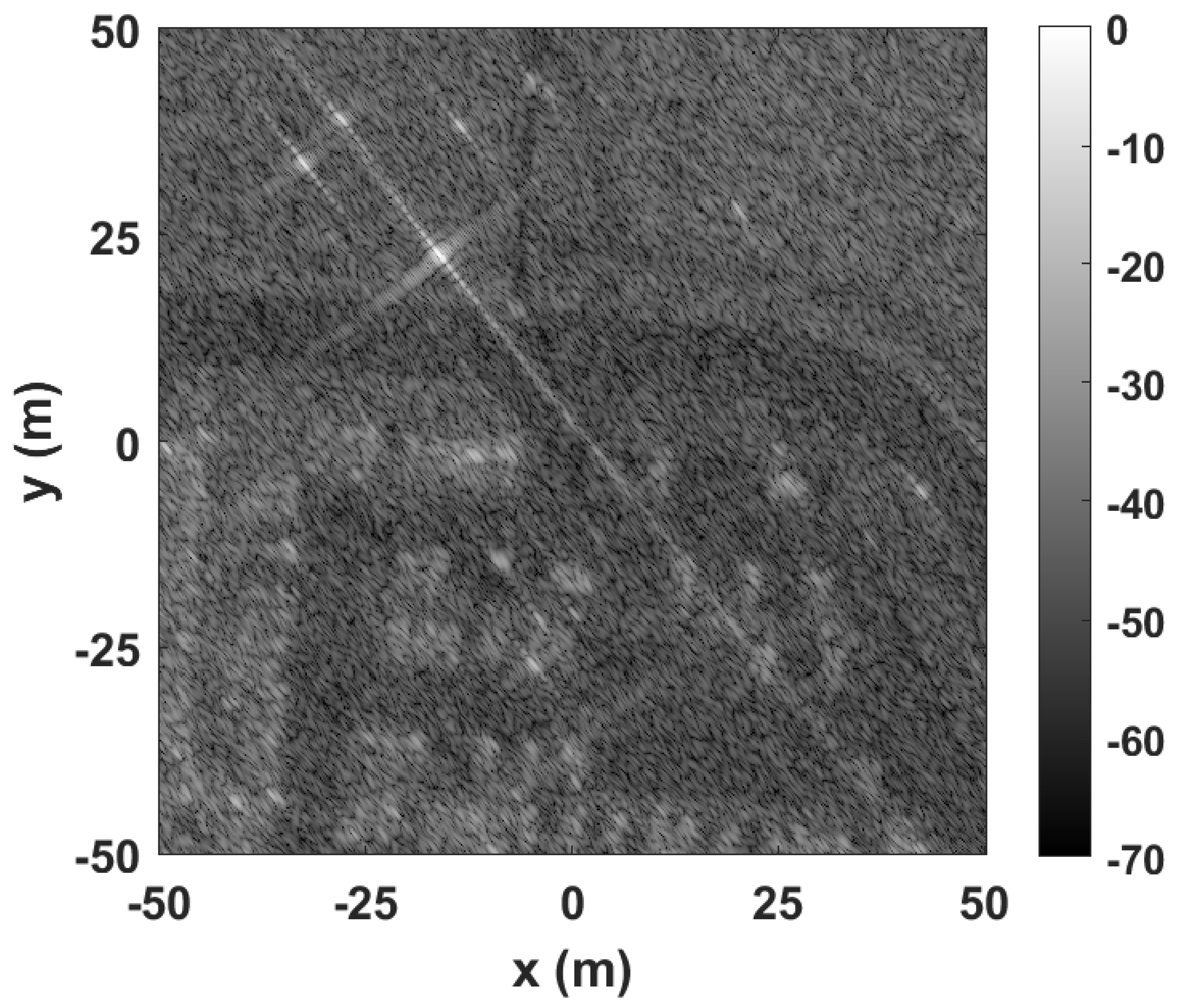
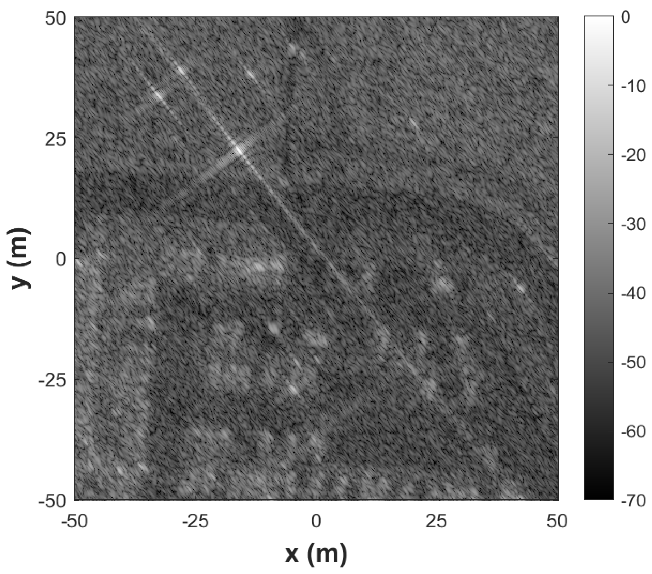
Two images can appear similar or equal to the human eye and still have very different values of SNR with large SSIM, as evidenced in Figure 1. Figure 1 shows two images: Figure 1 is the image generated using the Backprojection algorithm implemented with double-precision variables and the GOTCHA dataset at 39º. This image has an SSIM of 1.0 and an SNR of 145.66 dB. Figure 1 is generated using the Backprojection algorithm, where the variable that stores the image is truncated, resulting in a precision loss. This image has an SSIM of 0.99 and an SNR of 31.27 dB. Even though [7] states that SNR values above 100 dB are considered reasonable, Figure 1 has a SNR of 31.27 dB, compared to the 145.66 dB of Figure 1, and there is no discernible difference between the two images at naked eye, which is attested by the SSIM values, which are 0.99 and 1.0, respectively.

In this work, the MSE is used to compare the quality of the approximations during the development. However, the approximations are considered acceptable when the image generated using them has an SSIM above 0.99.

3. Approximation methodology

This work investigates approximations for the square root, sine, and cosine functions suitable for hardware designed for the Backprojection algorithm, minimizing the resources and execution time necessary for the algorithm. Most approximations are created as the best compromise between resources and precision without taking the application into account. In this work, the approximations are developed to be precise enough to satisfy the quality requisites, avoiding additional hardware.

Previous work has shown that the impact of reducing the word length on different variables of the Backprojection algorithm varies [1,3], which means that not all approximations require the same precision. Thus, the precision required for each approximation depends on the approximated function application.

The following steps were followed to develop and implement approximations for the square root, sine, and cosine functions and to determine the best candidates for the on-board architecture of the Backprojection algorithm:

Analysis of the domain and range of each function to be approximated. This analysis gives insight into the number of bits required for the fixed-point implementation and allows the observation of the function in its domain, facilitating the development of the approximation.
Explore different approximations, such as polynomial approximation using the Vandermonde matrix, linear interpolation for the square root, sine, and cosine functions, and Chebyshev polynomials for the sine and cosine functions. Polynomial approximation using the Vandermonde matrix provides the best fit for a certain curve, while linear interpolation calculates the line equation using the initial and final point of a curve. Therefore, polynomial approximation has more precision; however, it requires storing the slope and y-intercept for each function or subfunction. With linear interpolation, it is only necessary to store the points, requiring half the memory polynomial approximation for the same number of functions.
Explore optimum spacing vs. power of 2 spacing. Optimum spacing consists of having piecewise functions where the subfunctions’ domain is determined to minimize the MSE. It is the most precise approach; however, it requires additional calculations to map the input value into the correct subfunction. Furthermore, the computational complexity of calculating the optimum points increases exponentially as the number of points increases. Power of 2 spacing allows mapping the input value into the correct subfunction using the most significant bits without additional calculations. While less precise, it is faster and requires a smaller circuit to implement.
Floating-point implementation of the approximations. The approximations are first tested and implemented in floating-point, where their MSE is obtained. Only the best candidates are implemented in fixed-point.
Fixed-point implementation of the approximations. If the results obtained from the floating-point implementation are promising, the approximations are implemented in hardware, where the SSIM of the image is obtained. This iterative implementation process allows faster development and avoids implementing approximations without sufficient precision.

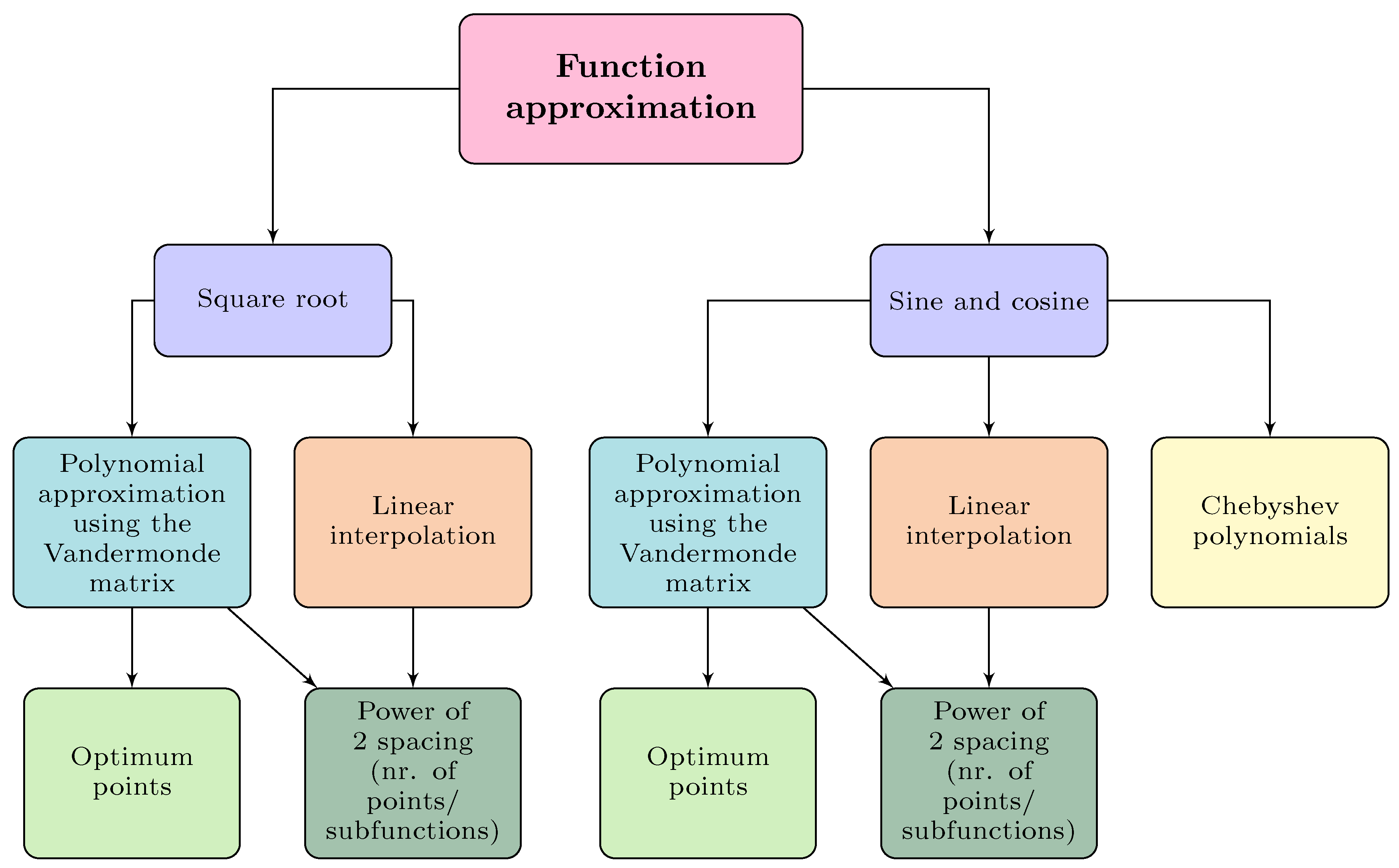
Figure 2 shows the approximations developed for each approximated function, such as polynomial approximation using the Vandermonde matrix and linear interpolation for the square root, sine and cosine functions, and Chebyshev polynomials for the sine and cosine functions. Polynomial and linear interpolation were developed using one function or a piecewise function with several subfunctions to increase the precision of the approximation. The domain of the subfunctions was chosen using two approaches: optimum points or power of 2 spacing. Optimum points are best suited for functions with curves, maximizing the precision of the approximation depending on their location. For instance, for a sine curve, it is best to increase the number of subfunctions when

x > \frac{π}{2}

. Power of 2 spacing means that the function’s domain is a power of 2. This method is better suited for hardware since it allows the identification of the subfunction that needs to be used for each input value using the most significant bits.

4. Trigonometric approximations

Approximations for the sine and cosine functions have been proposed over the years. Taylor Series is one of them; however, it converges slower than other series-based methods. Chebyshev polynomials are a better alternative to the Taylor Series since they converge faster with the same number of terms [8]. The CORDIC algorithm [9] is an iterative algorithm used to calculate hyperbolic and trigonometric functions and has good results when no hardware multipliers are available, such as in FPGAs. CORDIC calculates one bit per iteration. Methods such as linear and polynomial approximation can be applied to many function, including trigonometric functions.

The Backprojection algorithm was modified by changing the input domain of the sine and cosine functions using variable substitution, as described in the next section. The sine and cosine functions were approximated using Chebyshev polynomials, polynomial approximation using the Vandermonde matrix, and linear interpolation considering the new function domain.

The trigonometric functions were implemented using the following pre-defined fixed-point configurations: Q4.23 for the input and Q2.25 for the output [3].

4.1. Modifications to the Backprojection algorithm

In software, the implementations of sine and cosine from the math.h library are designed to provide full precision within the representation range of floating-point variables. Approximations, however, usually provide less precision than these implementations. Trigonometric approximations have limited domains, typically within the first quadrant, and start to deviate as the input values increase [10]. The input values can be mapped into the other quadrants for periodic functions such as the sine and cosine. This means that it is possible to approximate a sine wave in the domain

[0, 2 π]

using only the first quadrant, or

[0, \frac{π}{2}]

. Calculating the cosine using a sine function is possible, and vice-versa. However, additional steps are necessary when the input values are outside the domain

[0, 2 π]

. The module function maps larger values into the function’s domain, removing additional turns of

2 π

. This function uses a division operation, which is an expensive operation in hardware. Avoiding the module operation requires changing the function’s domain.

In Algorithm 1, line 13 shows the calculation of the input value for the trigonometric functions where the value is multiplied explicitly by

π

. Removing this multiplication transforms the domain of the trigonometric functions from

[0, 2 π]

[0, 2]

. With a variable substitution, instead of

sin (x)

, the input variable is replaced by

y = π x

, and the function is now

sin (y)

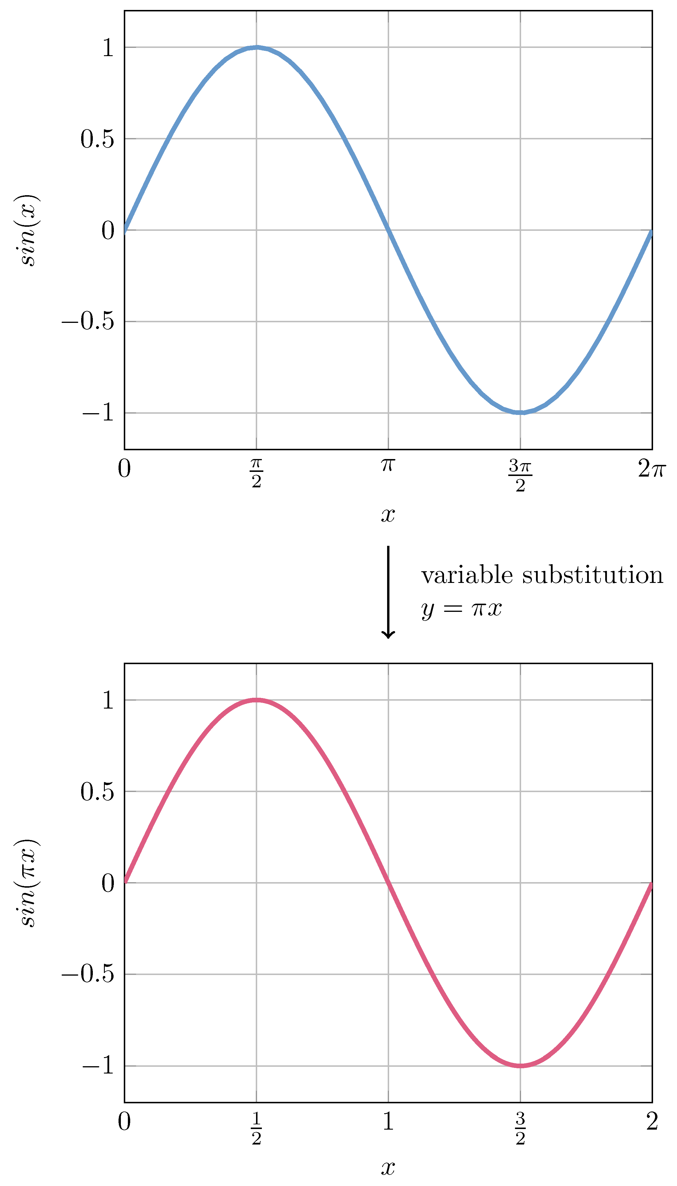
. This can be seen in Figure 3.

Adjusting the domain of the function changes the module operation from fmod(value, $2 π$ ) to fmod(value, 2), which is reduced to bitwise operations in hardware.

The variable substitution and consequent domain alteration remove an expensive operation and allow the use of approximations without compromising the precision with larger input values. Furthermore, the quadrant of an angle can be determined with the two most significant bits. The alteration also requires the implementation of different approximations since most available approximations are designed for the traditional domain of

[0, 2 π]

4.2. Chebyshev polynomials and Bessel functions approximation

Series approximations, such as Taylor Series, are used to approximate functions using sums of terms. The main disadvantage of this method is that many terms can be required depending on the necessary accuracy. This also means that more bits are needed to represent the powers of the input value. Chebyshev polynomials and Bessel functions can be used for function approximation and are more accurate when compared to the Taylor Series approximation with the same number of terms [8].

Approximations using Chebyshev polynomials for trigonometric functions, exponential, logarithms, and square root, among others, are provided in [10]. Depending on the input and precision, there are different approximations for the sine and cosine functions. For this work, the relevant approximations are the ones that follow the variable substitution described in Section 4.1, with the

π

outside of the calculation, as shown in Equation 1 [10].

\begin{matrix} \begin{matrix} cos (β π x) & \approx P (X^{2}) \\ β & = \frac{1}{4} \end{matrix} \end{matrix}

(1)

The cos3820 approximation has six different variations, ranging from four to nine coefficients [10]. More accurate approximations require more terms, as expected. This implementation uses the less precise variation, named cos3820, with four coefficients, as shown in Equation 2.

\begin{matrix} \begin{matrix} cos 3820 (β π x) & \approx c_{1} + c_{2} \times x^{2} + c_{3} \times x^{4} + c_{4} \times x^{6} \\ c_{1} & = 0.99999996738 \\ c_{2} & = - 0.30842416558 \\ c_{3} & = 0.01584968416 \\ c_{4} & = - 0.00031872783 \end{matrix} \end{matrix}

(2)

The input value of this approximation is

β π x

, where

β = \frac{1}{4}

, therefore, the domain of this approximation is

[0, 2]

. This requires a multiplication of the input value by 4.

A variation of this approximation where the

c_{4}

term was omitted was also tested. Table 1 shows that both implementations satisfy the quality requirements, with SSIM over 0.99. The impact of the MSE in the SSIM of the final image is significantly less when compared to the square root approximations. While with the square root approximations, the MSE needed to have an order of magnitude of

10^{- 8}

to generate images with acceptable SSIM, it is possible to generate an image with an acceptable SSIM with a sine approximation with an order of magnitude of

10^{- 5}

. Furthermore, Table 1 shows that a difference of 3.07624 × 10⁻⁵ in the MSE translates to a difference of only 0.0005 in the SSIM.

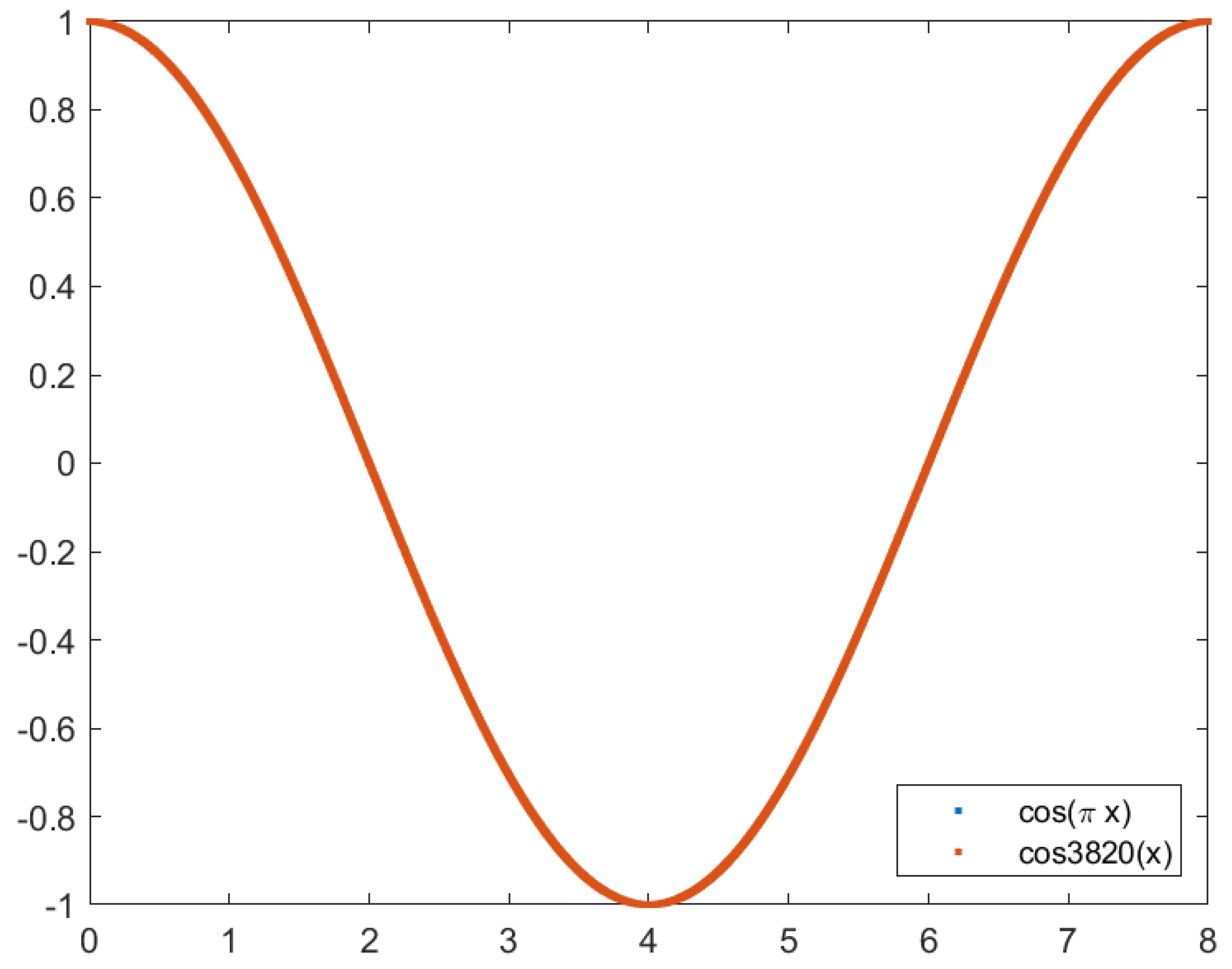
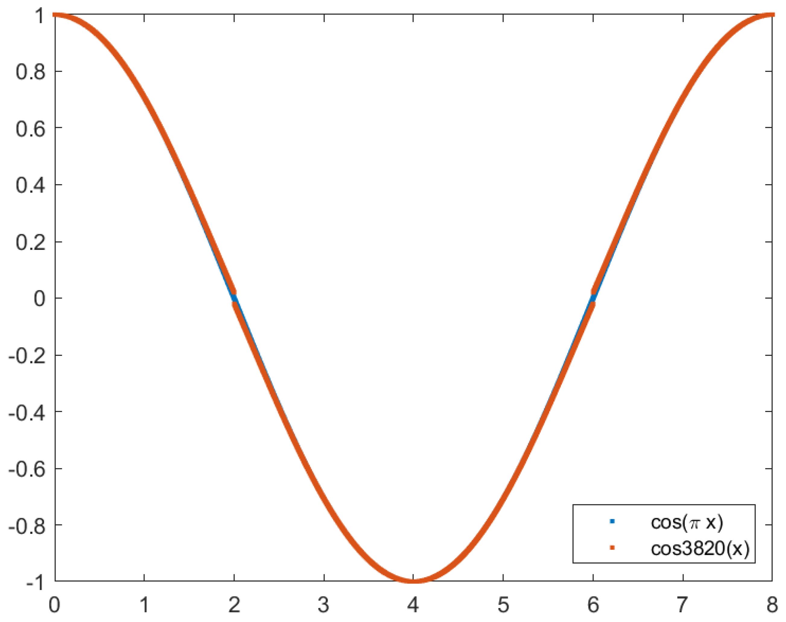
Figure 4 and Figure 5 show the image generated using the Backprojection algorithm and the cosine approximation using Chebyshev polynomials and Bessel functions with four and three terms, respectively. Figure 6 and Figure 7 show the plot of the cosine function (in red) and the Chebyshev approximation (in blue) with four terms and three terms, respectively. While it is impossible to see differences in the four-term approximation, the same is not valid for the three-term approximation. Noticeably, for

x = 2

and

x = 6

when the cosine approaches zero, the approximation is never zero.

4.3. Sine approximation using polynomial approximation using the Vandermonde matrix approximation

The Chebyshev approximation satisfied the quality requisites; however, it has one disadvantage: it cannot be used for all quadrants. Even though the cosine function is a periodic function and the first quadrant is enough to calculate the results in every domain, this implies additional logic and circuit area to map the input angle into the new value.

A polynomial approximation using the Vandermonde matrix is used to obtain a polynomial that best fits a function’s curve. This means that it can be used in the four quadrants, unlike the Chebyshev approximation, which can only be used in the first quadrant. The coefficients for the polynomial approximation are obtained using the polyfit function from MATLAB.

Using one function to approximate the sine curve in the first quadrant, the coefficients are the following:

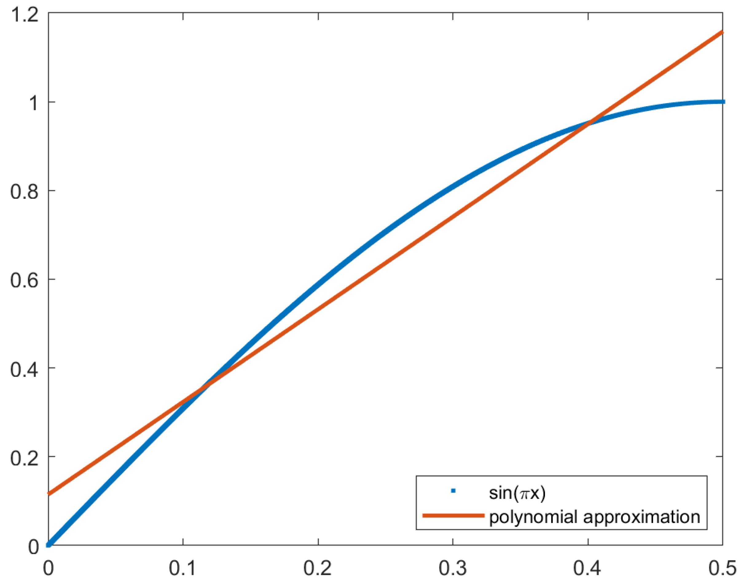
\begin{matrix} m & = 2.08739609906403 \\ b & = 0.114770610981535 \end{matrix}

(3)

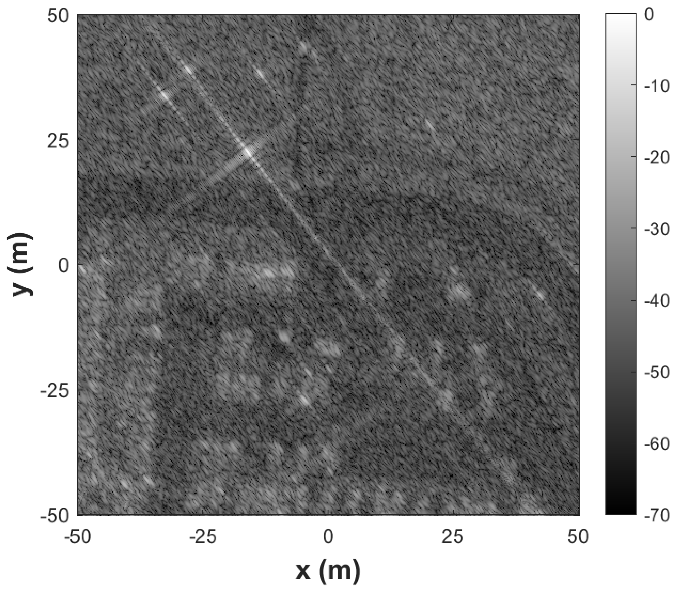
The approximation function is in red in Figure 8, with the sine function in blue. This approximation has an MSE of 3.94000 × 10⁻³, and the image generated has an SSIM of 0.95962; therefore, it does not meet the requirements. Figure 9 shows the image generated using the Backprojection algorithm and this approximation.

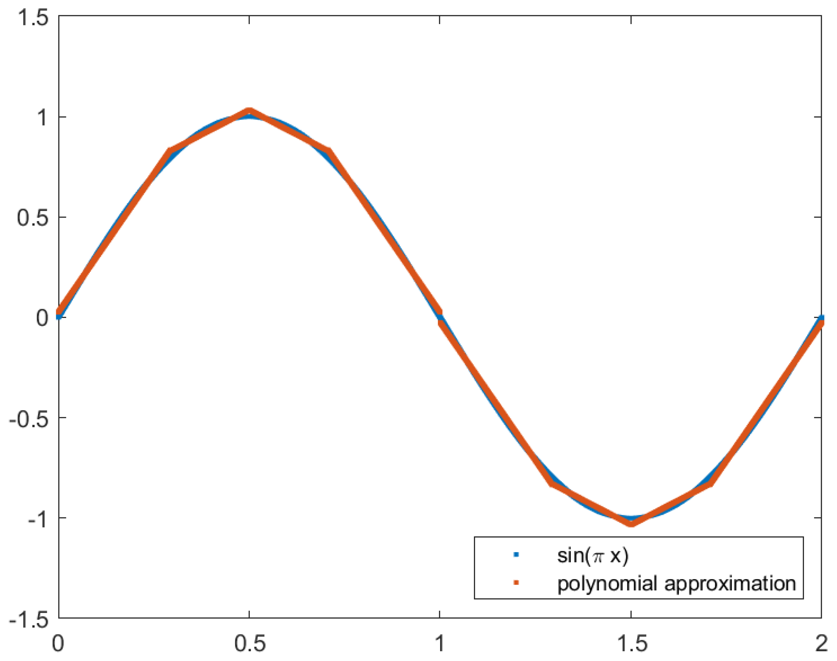
While observing the sine wave, we can conclude that the wave is similar to a line between

x = 0

and

x = 0.2

, curving as the x increases. For this reason, the next step is to increase the number of subfunctions to accommodate subdomains where the curve deepens.

4.3.1. Sine approximation using polynomial approximation using the Vandermonde matrix and subfunctions with optimum points

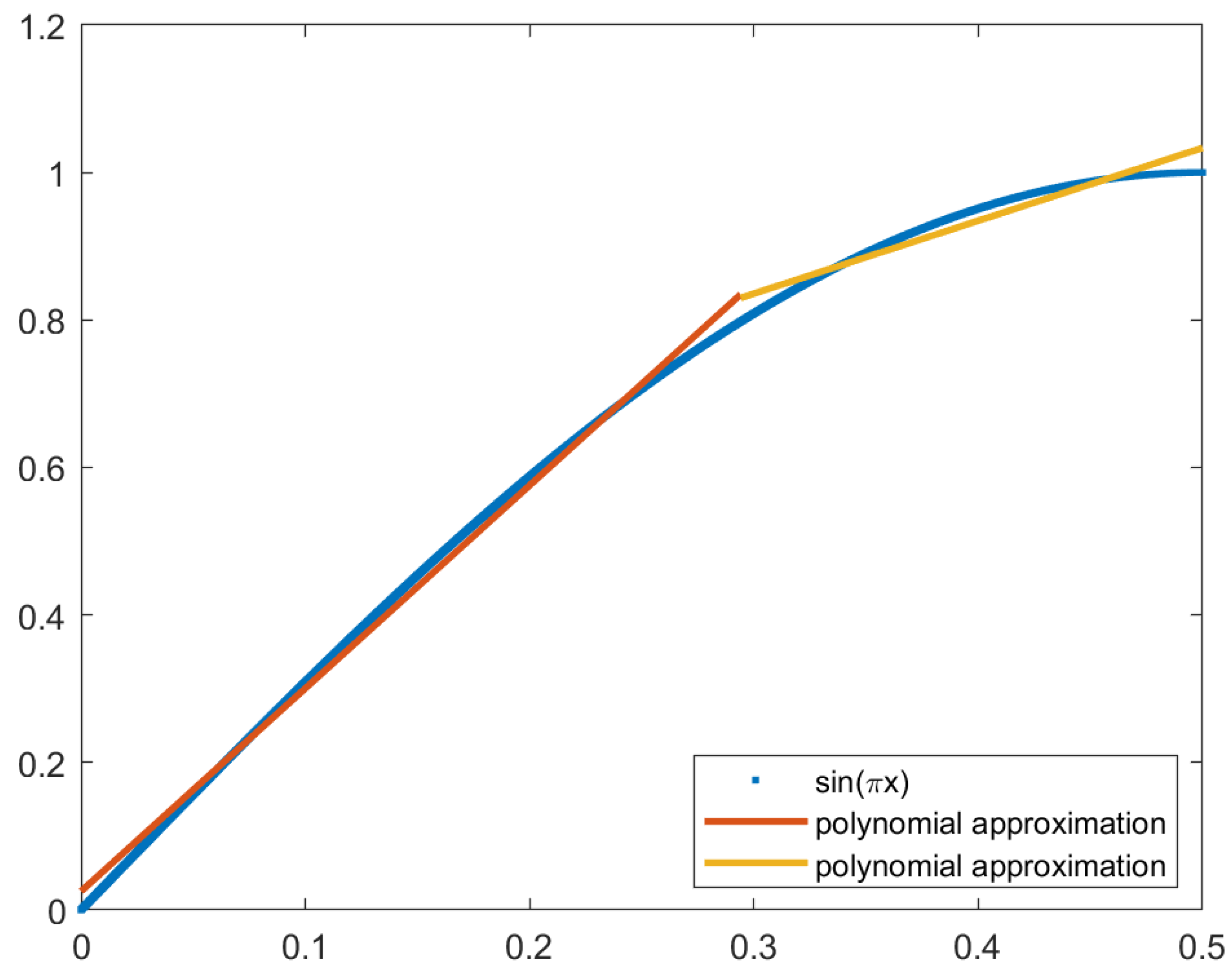
Polynomial interpolation with a piecewise function increases the precision of the approximation. The challenge when creating a piecewise function for the sine function is deciding the domains of the subfunctions. Observing the sine curve shows that the function is similar to a line when

x \in [0, 0.25]

, then the curve deepens. This means that it would be beneficial to increase the number of subfunctions when

x \in] 0.25, 0.5]

. The optimum point was determined by calculating the MSE of the piecewise function with every possible domain for the subfunctions. The step between possible optimum points was 0.0001.

Using two subfunctions, the optimum point is when

x = 0.2941

, with an MSE of 2.06271 × 10⁻⁴. The piecewise function is given by:

f (x) = \{\begin{matrix} 2.75271389433335 x + 0.0252414129216198 & if x \in [0, 0.2941 [ \\ 0.988048356099987 x + 0.539403210517531 & if x \in [0.2941, 0.5] \end{matrix}

(4)

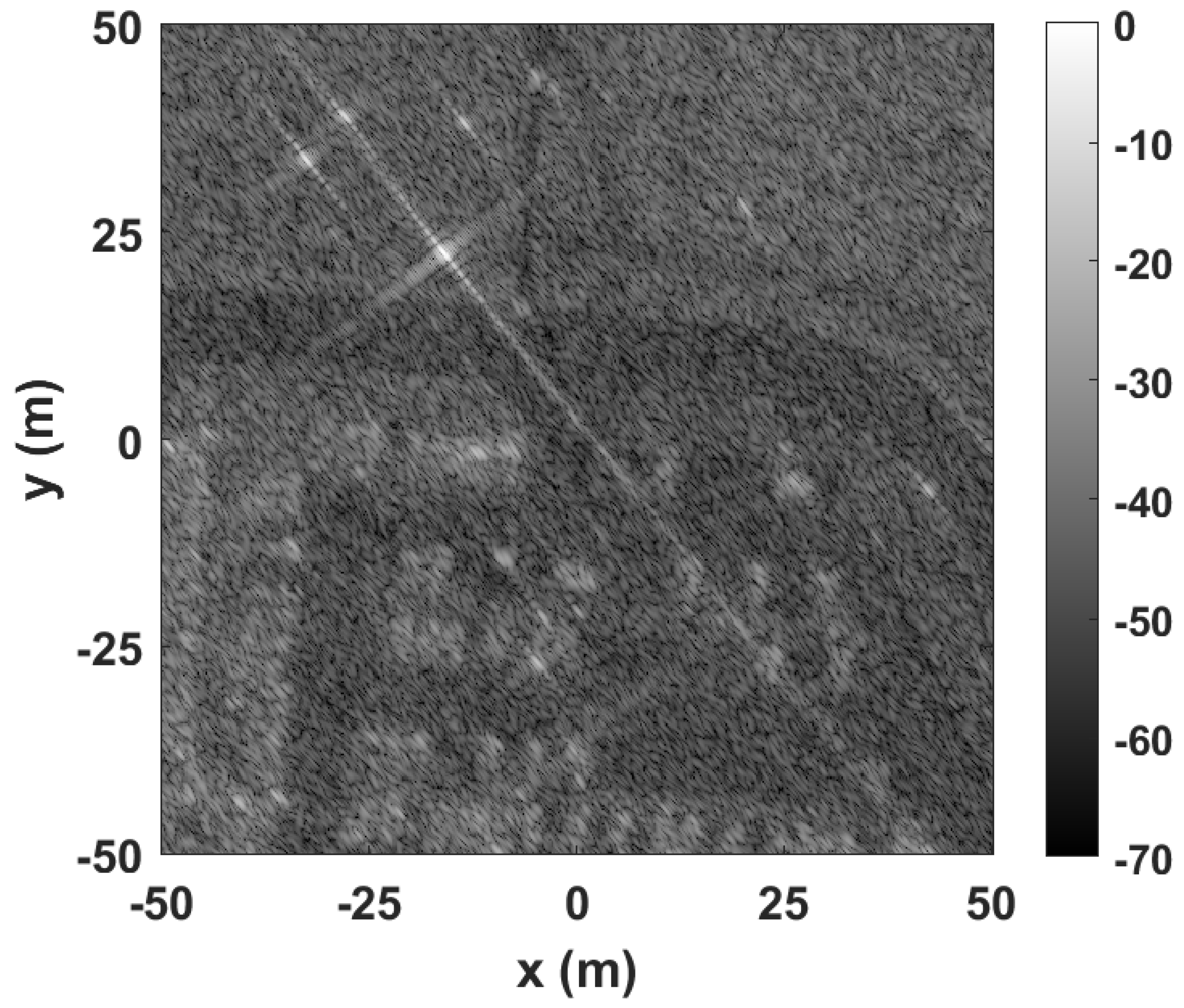
The piecewise function with two subfunctions is plotted in Figure 10, with the original function in red and the approximation in blue. Figure 11 shows the image generated using this approximation, with an SSIM of 0.99314.

4.3.2. Sine approximation using polynomial approximation using the Vandermonde matrix and subfunctions with a power of 2 spacing

The advantage of the optimum point implementation is guaranteeing the lowest possible MSE for the number of subfunctions. This implementation, however, requires additional operations to map the input value into each subfunction, which is costlier in hardware. An alternative to this approach is to use a power of 2 spacing between subfunctions, which allows the identification of the subfunction using the most significant bits of the input value.

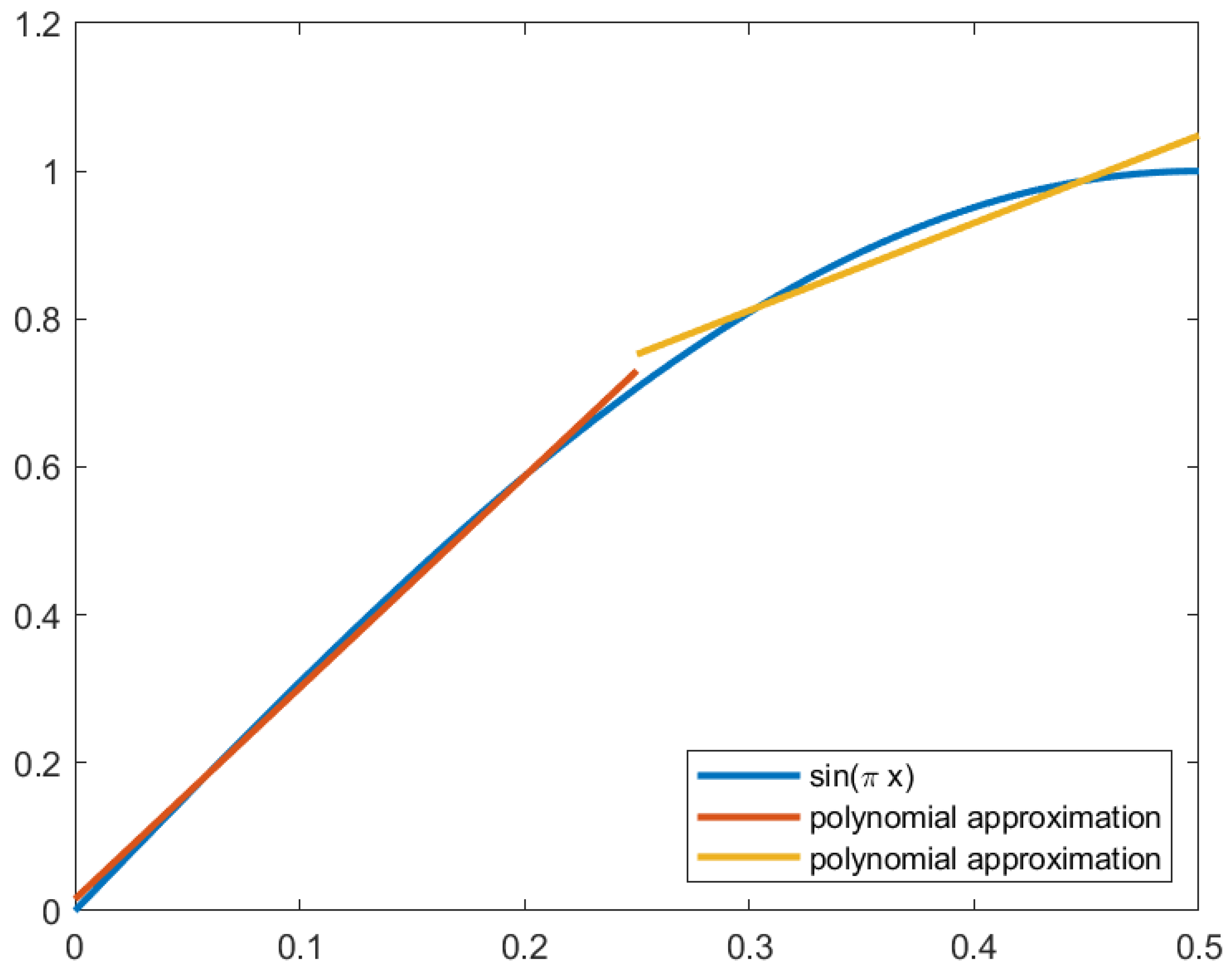
We calculated the MSE for each piecewise function using a power of 2 spacing, where the power of 2 varied between -2 and -6; that is, the spacing ranged from 0.25 to 0.015625. The MSE of these approximations is shown in Table 2. As seen in Section 4.3.1, it is possible to generate acceptable images with an MSE with an order of magnitude of

10^{- 4}

. The approximation satisfying this condition uses two subfunctions and is marked in pink in Table 2. The piecewise function is given by:

f (x) = \{\begin{matrix} 2.857939136510715 x + 0.01568075903486843 & if x \in [0, 0.25] \\ 1.183797150779596 x + 0.4563921975630670 & if x \in [0.25, 0.5] \end{matrix}

(5)

The piecewise function is plotted in Figure 14. The image generated by this approximation is shown in Figure 13 and has an SSIM of 0.99246.

4.4. Sine approximation using linear interpolation with power of 2 spacing

Linear interpolation uses points to calculate the line equation, calculating the interpolated value using the stored points. Thus, it requires half the memory than the polynomial approximation using the Vandermonde matrix, which requires the slope and the y-intercept. Polynomial approximation provides a better fit, despite needing more memory. This section compares linear interpolation to polynomial approximation, evaluating the tradeoff between approximation precision and required memory. Linear interpolation is calculated using Lagrange’s polynomial:

f (x) = y_{0} + \frac{y_{1} - y_{0}}{x_{1} - x_{0}} (x - x_{0})

(6)

Division operations are expensive in hardware. However, this operation can be replaced by a bitwise operation with a power of 2 spacing.

Linear interpolation was tested with a power of 2 spacing, where the power of 2 ranged from

2^{- 1}

2^{- 6}

, that is, from 0.5 to 0.015625. The MSE obtained for each approximation is shown in Table 3. With this approximation, the smaller number of functions needed to obtain an MSE with an order of magnitude of

10^{- 4}

is four, which results in an MSE of 9.84239 × 10⁻⁵. Figure 15 shows the image generated using linear interpolation with five points. This image has an SSIM of 0.99562.

The linear interpolation approximation requires five points, while the polynomial approximation using the Vandermonde matrix requires two subfunctions. Therefore, linear interpolation requires storing five values, while polynomial approximation requires four.

5. Square root approximation

There are methods of computing square roots that require a first guess, such as the Babylonian [11] and Newton’s methods [12]. These methods require a first guess and then converge to the result iteratively, increasing the result’s precision with the number of iterations. The nearest perfect square method requires finding the previous and next nearest perfect squares, which is challenging. Furthermore, it requires a division operation, which is expensive in hardware. Other works, specifically for hardware, use a table-based polynomial function [13].

The square root approximations proposed in this section are implemented with the following fixed-point configurations for input and output values: Q28.19 for the input and Q15.33 for the output [3].

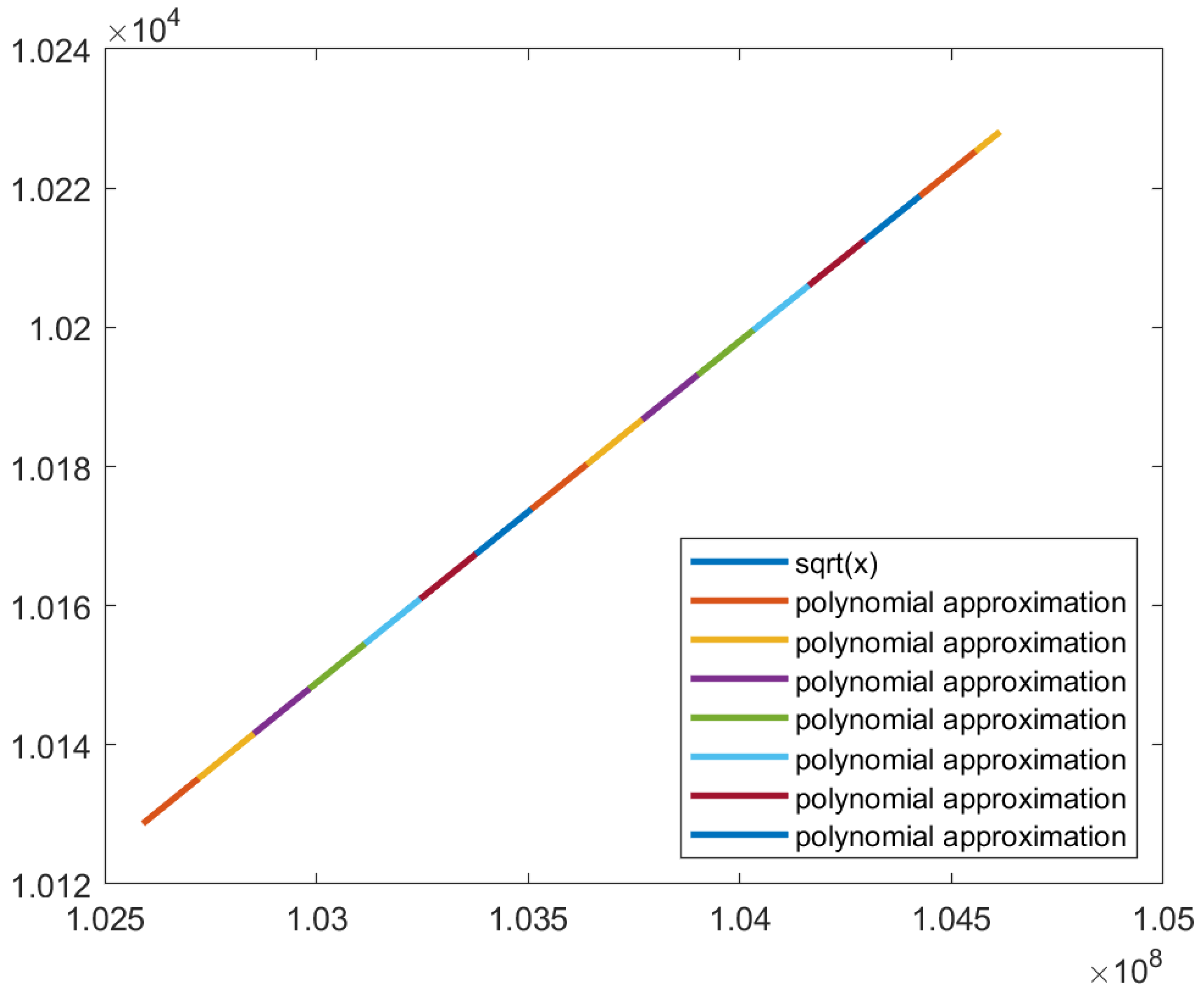
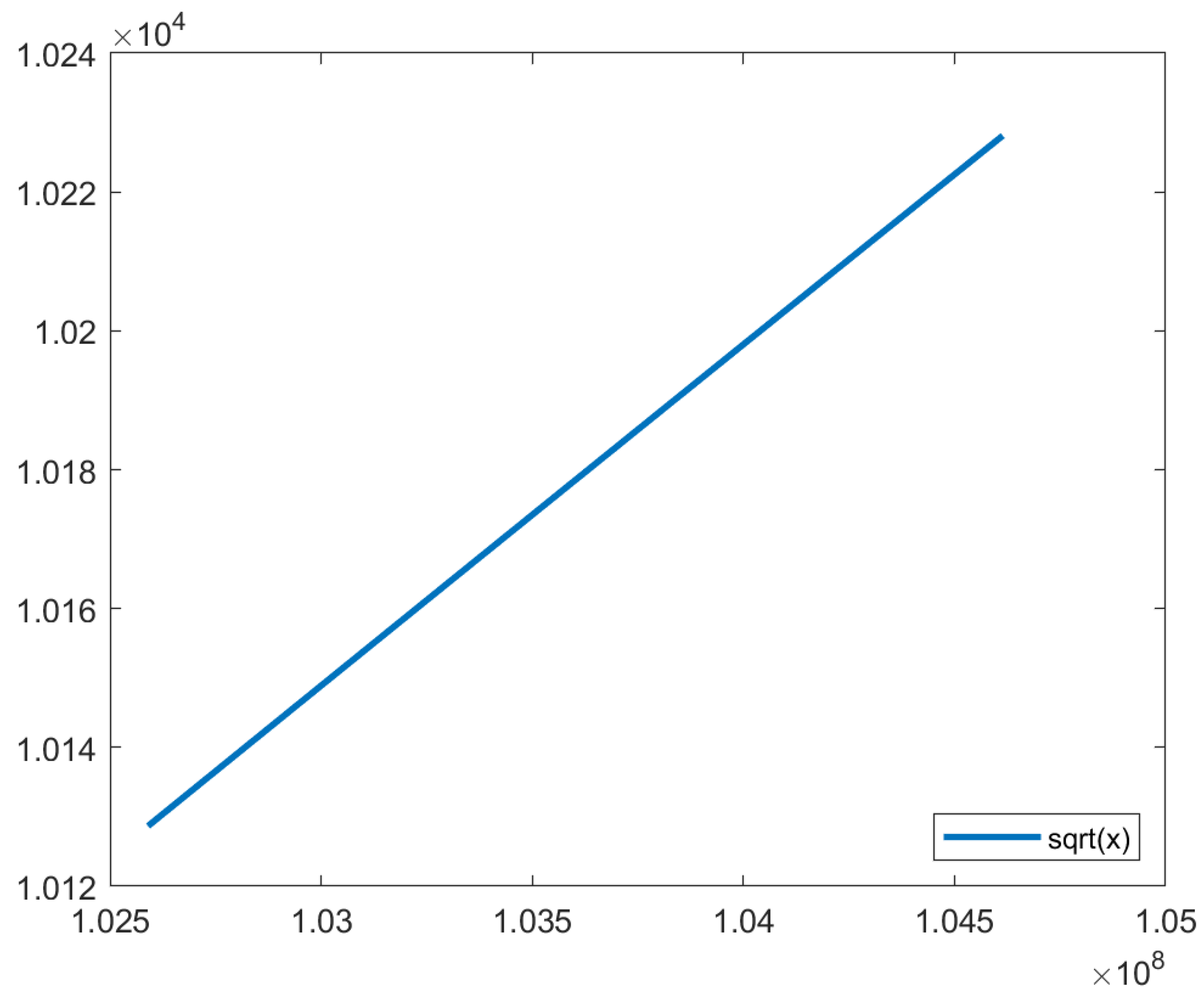
In Figure 16, it is possible to conclude that the square root function in the algorithm’s domain is similar to a line to the naked eye. Therefore, polynomial approximation using the Vandermonde matrix and linear interpolation have the potential for approximating the square root function in the algorithm’s domain with the required precision to achieve an acceptable SSIM.

5.1. Square root approximation with polynomial approximation using the Vandermonde matrix

Polynomial approximation with the Vandermonde matrix provides the slope and y-intercept for a line. Using one function to interpolate the square root function in its domain, the coefficients are the following:

\begin{matrix} m & = 4.91234451079138 \times 10^{- 05} \\ b & = 5089.17912997872 \end{matrix}

(7)

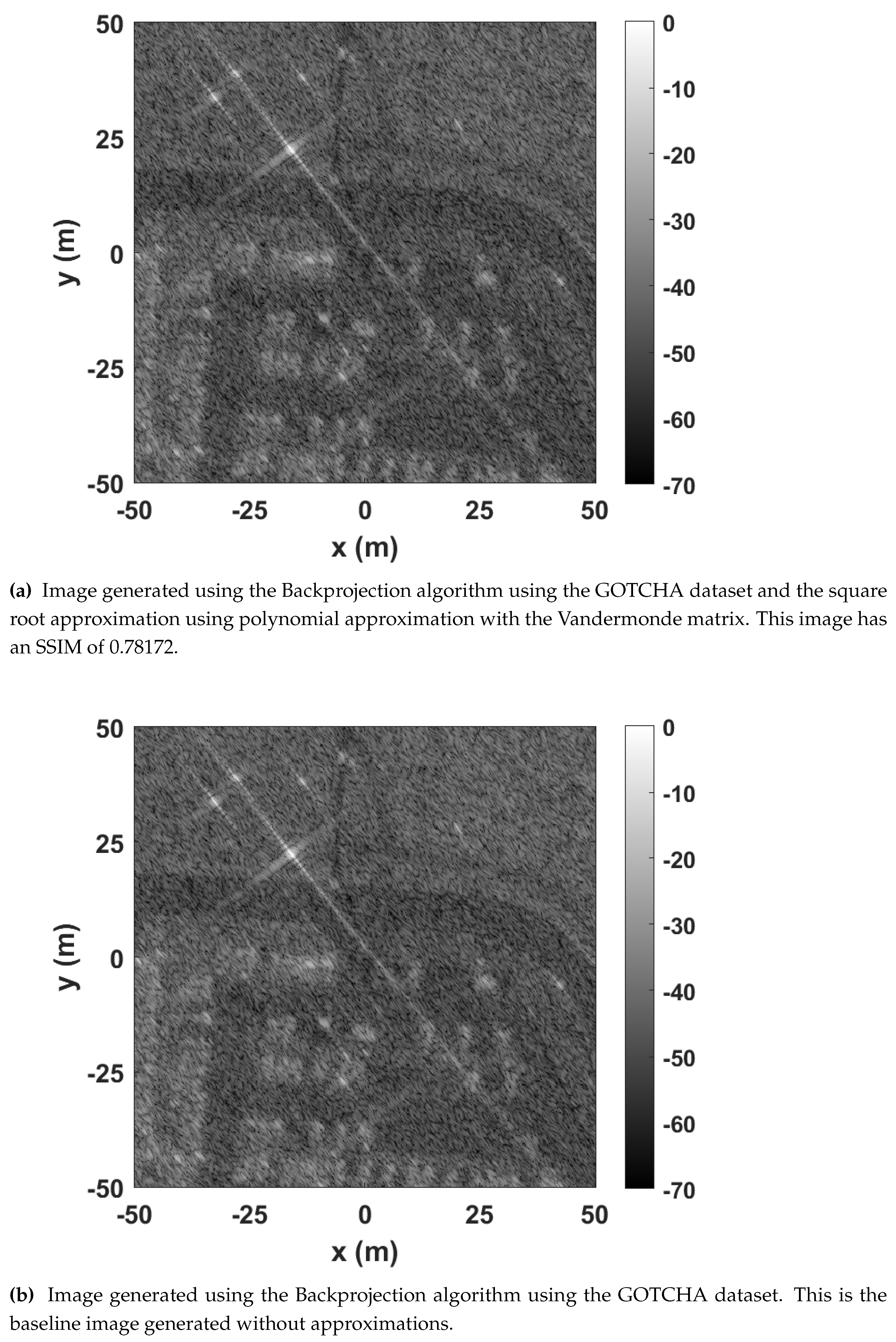
This approximation has an MSE of 1.50845 × 10⁻³, and the image generated has an SSIM of 0.78172. The low SSIM is explained by the speed of light acting as a scaling factor, as seen in line 13 of Algorithm 1, increasing the impact of the approximation’s errors. This image is compared to the baseline in Figure 17, where Figure 17 shows the image generated using the square root approximation and Figure 17 shows the baseline image. Even though the images appear equal, Figure 17 is distorted. The distortion would be more apparent for circular SAR using multiple angles.

Since one function is not precise enough to obtain an SSIM above 0.99, the next step was to use piecewise functions and increase the number of subfunctions.

5.2. Polynomial approximation using the Vandermonde matrix with subfunctions using optimum points

Polynomial approximation using the Vandermonde matrix with subfunctions was used to increase the precision of the approximation. The domain of each function was calculated using optimum points, similar to the sine approximation. The optimum points were tested in steps of 674, and the optimum one was found to be

x = 103598296

. The coefficients obtained are the following:

f (x) = \{\begin{matrix} 4.9287113525650 \times 10^{- 5} x + 5076.74510104271 & if x \in [102589992, 103598296] \\ 4.9004093225725 \times 10^{- 5} x + 5101.60453039511 & if x \in] 103598296, 104614224] \end{matrix}

(8)

The piecewise function has an MSE of 7.95870 × 10⁻⁵, and the image has an SSIM of 0.91314, as shown in Table 4. The last step was to try with three subfunctions.

Figure 18. Image generated using the Backprojection algorithm using the GOTCHA dataset and the square root approximation using polynomial approximation with the Vandermonde matrix with two subfunctions. This image has an SSIM of 0.91314.

Figure 19. Plot of the piecewise function with two functions generated using polynomial approximation with the Vandermonde matrix with optimum points.

The optimum points for the polynomial approximation using a piecewise function with three subfunctions were

x = 103237736

and

x = 103925964

, and the piecewise function is given by:

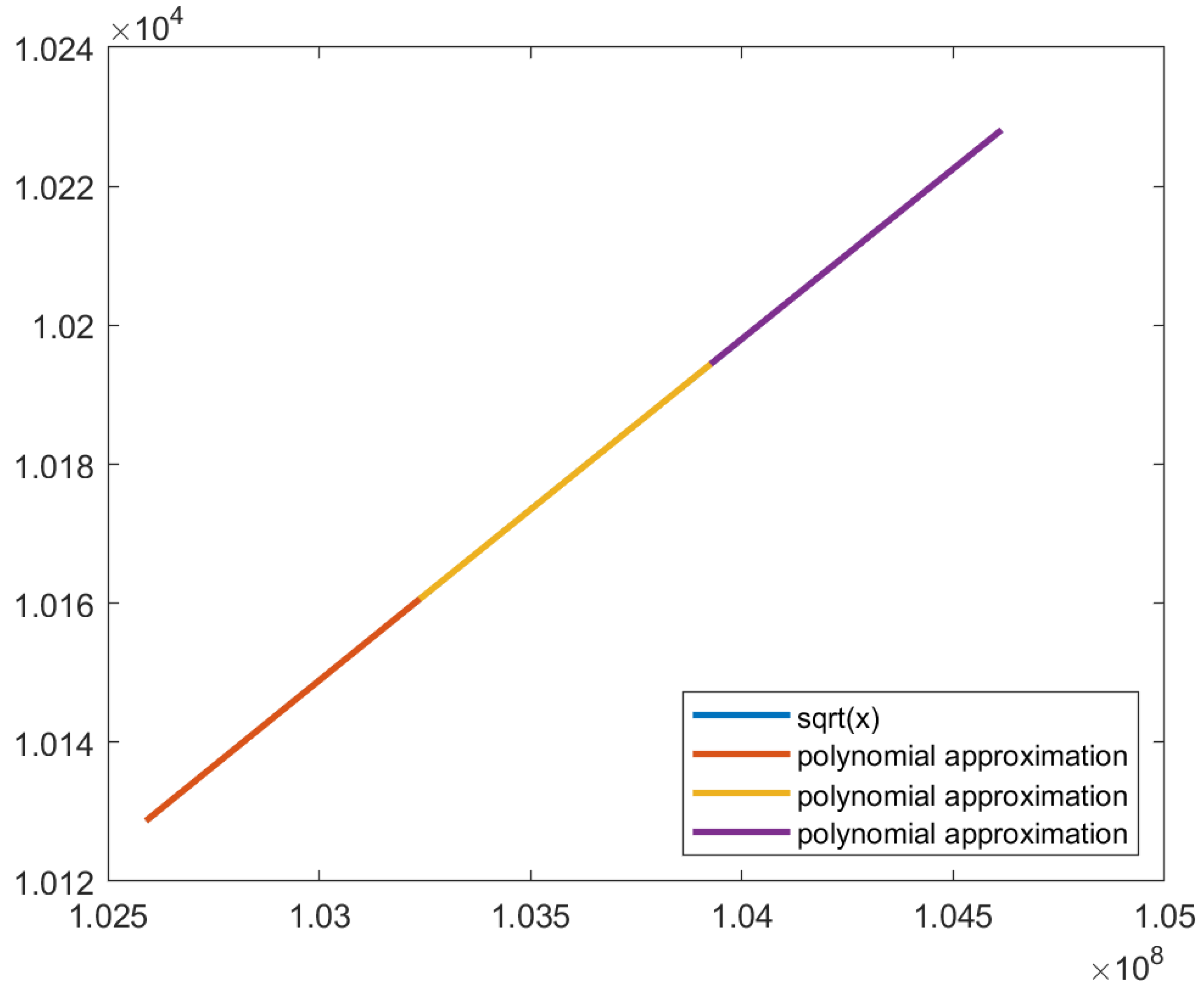
f (x) = \{\begin{matrix} 4.9287113525650 \times 10^{- 5} x + 5072.31557678833 & if x \in [102589992, 103237736] \\ 4.9127937530577 \times 10^{- 5} x + 5088.74955136983 & if x \in] 103237736, 103925964 [ \\ 4.8965531911339 \times 10^{- 5} x + 5105.62763875162 & if x \in [103925964, 104614224] \end{matrix}

(9)

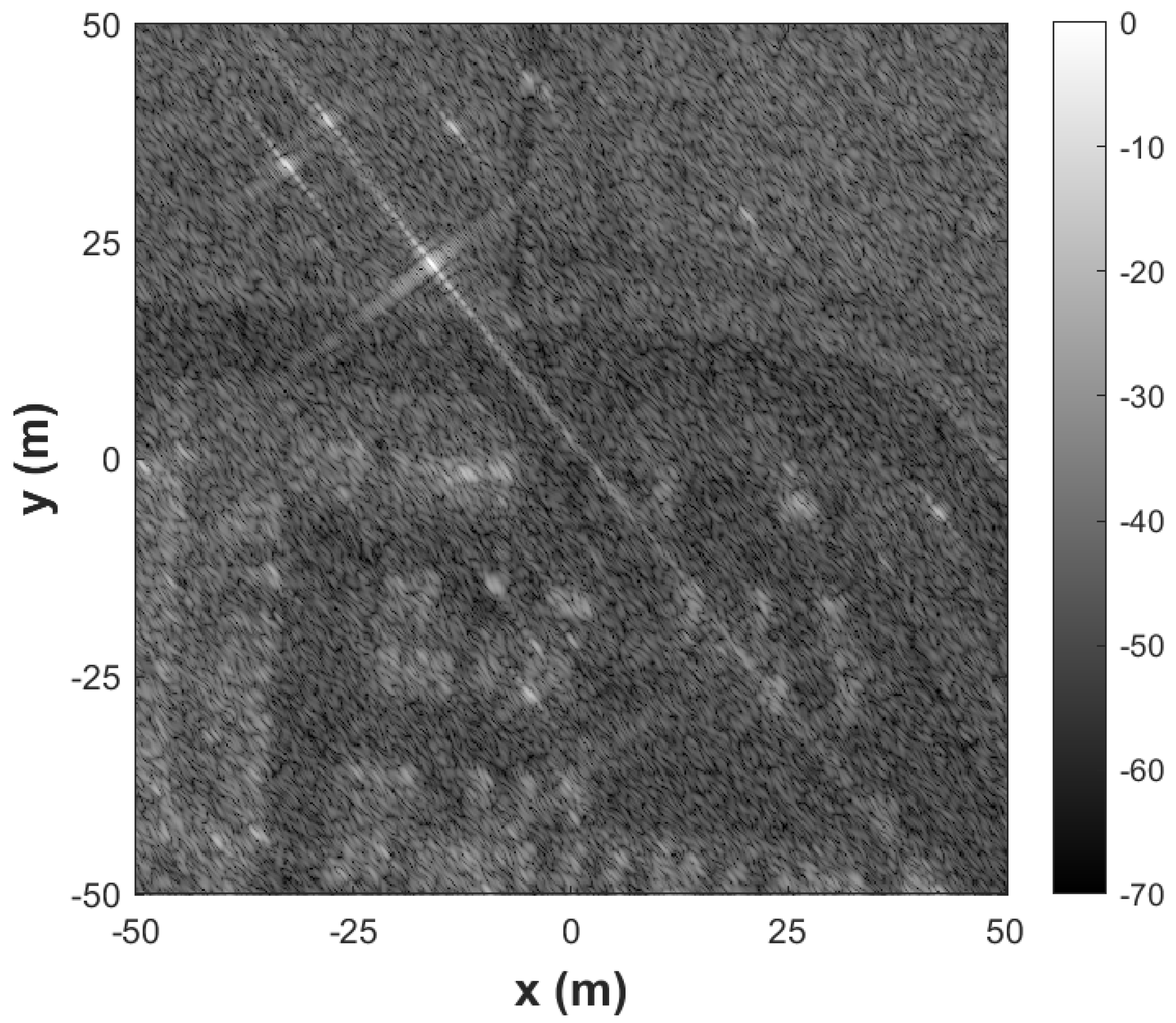
Figure 20 shows the plot of the subfunctions used to approximate the square root function. Figure 21 shows the image generated by this approximation. This approximation has an MSE of 1.61760 × 10⁻⁵ and an SSIM of 0.95851. The MSE and SSIM of the three polynomial approximations using the Vandermonde matrix approximations are shown in Table 4.

5.3. Second-degree polynomial approximation using the Vandermonde matrix with subfunctions using power of 2 spacing

Increasing the number of optimum points is not feasible due to the computation complexity of their calculation. Therefore, it is best to increase the number of subfunctions with a power of 2 spacing. It was not possible to obtain a suitable approximation for the square root with three optimum points; hence it is necessary to have an approximation with an MSE inferior to 1.61760 × 10⁻⁵.

Second-degree polynomial approximations using the Vandermonde matrix are inadequate for the square root approximation since the function’s domain already requires 49 bits for the square root input and output, and the input squared would require more bits and larger multipliers. However, the floating-point implementation of this approximation can be used to obtain an estimate regarding the necessary MSE to obtain an image that satisfies the image quality requirements.

The second-degree polynomial approximation for the square root function in the function’s domain is given by:

\begin{matrix} \begin{matrix} f (x) & = c_{1} \times x^{2} + c_{2} \times x + c_{3} \\ c_{1} & = - 3.3383 \\ c_{2} & = 3.7565 \\ c_{3} & = - 0.0243 \end{matrix} \end{matrix}

(10)

This approximation has an MSE of 5.55805 × 10⁻⁹ and an SSIM of 0.99996. This MSE is used as an indicator for the study of the polynomial approximation using the Vandermonde matrix with a power of 2 spacing. Even without a direct relation between the MSE and the SSIM, the approximations developed in this document indicate a strong relation between both. Therefore, we are looking for approximations with an MSE closer to 5.55805 × 10⁻⁹ and smaller than 1.61760 × 10⁻⁵. Notwithstanding, the SSIM value is still calculated for the best candidates.

5.4. Polynomial approximation using the Vandermonde matrix with subfunctions using power of 2 spacing

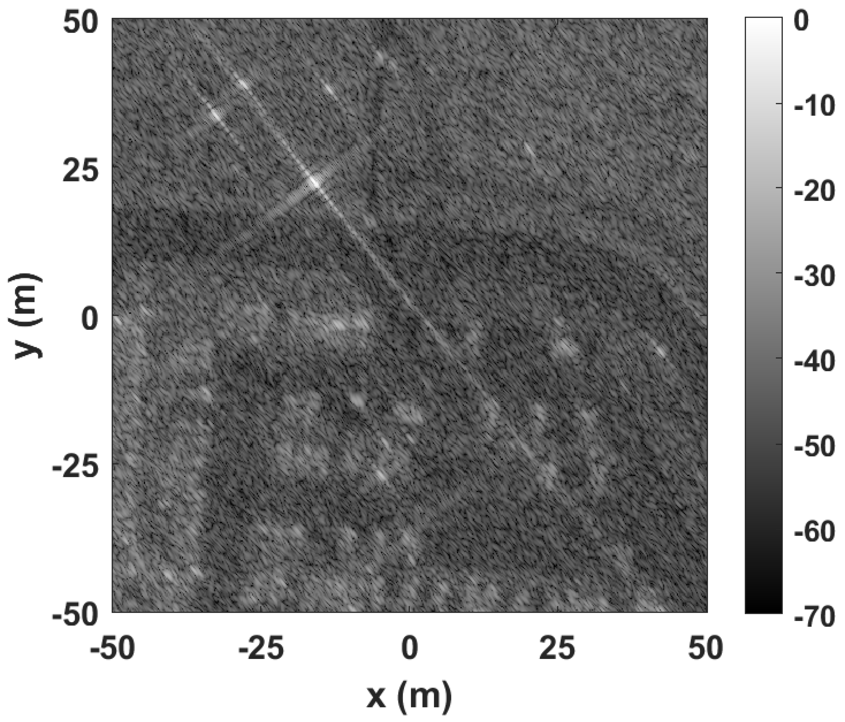
Polynomial approximations using the Vandermonde matrix with different numbers of subfunctions were used to increase the precision of the approximation. Evidence showed that three subfunctions do not provide enough precision to satisfy the quality requirements. Therefore, this approximation is tested with 4 to 989 subfunctions. These subfunctions correspond to a power of 2 spacing ranging from

2^{11}

2^{19}

. The MSE of each approximation is shown in Table 5.

The second-degree polynomial approximation provided insight regarding the MSE value needed to satisfy the quality requirements, which would be closer to 5.55805 × 10⁻⁹ and smaller than 1.61760 × 10⁻⁹. The numbers of subfunctions that satisfy these conditions are highlighted in pink in Table 5.

First, the piecewise function with eight subfunctions was implemented and tested. The SSIM of this approximation is 0.98916, failing to satisfy the requirements. This excludes the approximations with four and eight subfunctions. Then, the approximation with 16 subfunctions was tested, resulting in an SSIM of 0.99436. Therefore, at least 16 subfunctions are needed to satisfy the quality requirements and to generate an image with an SSIM above 0.99. 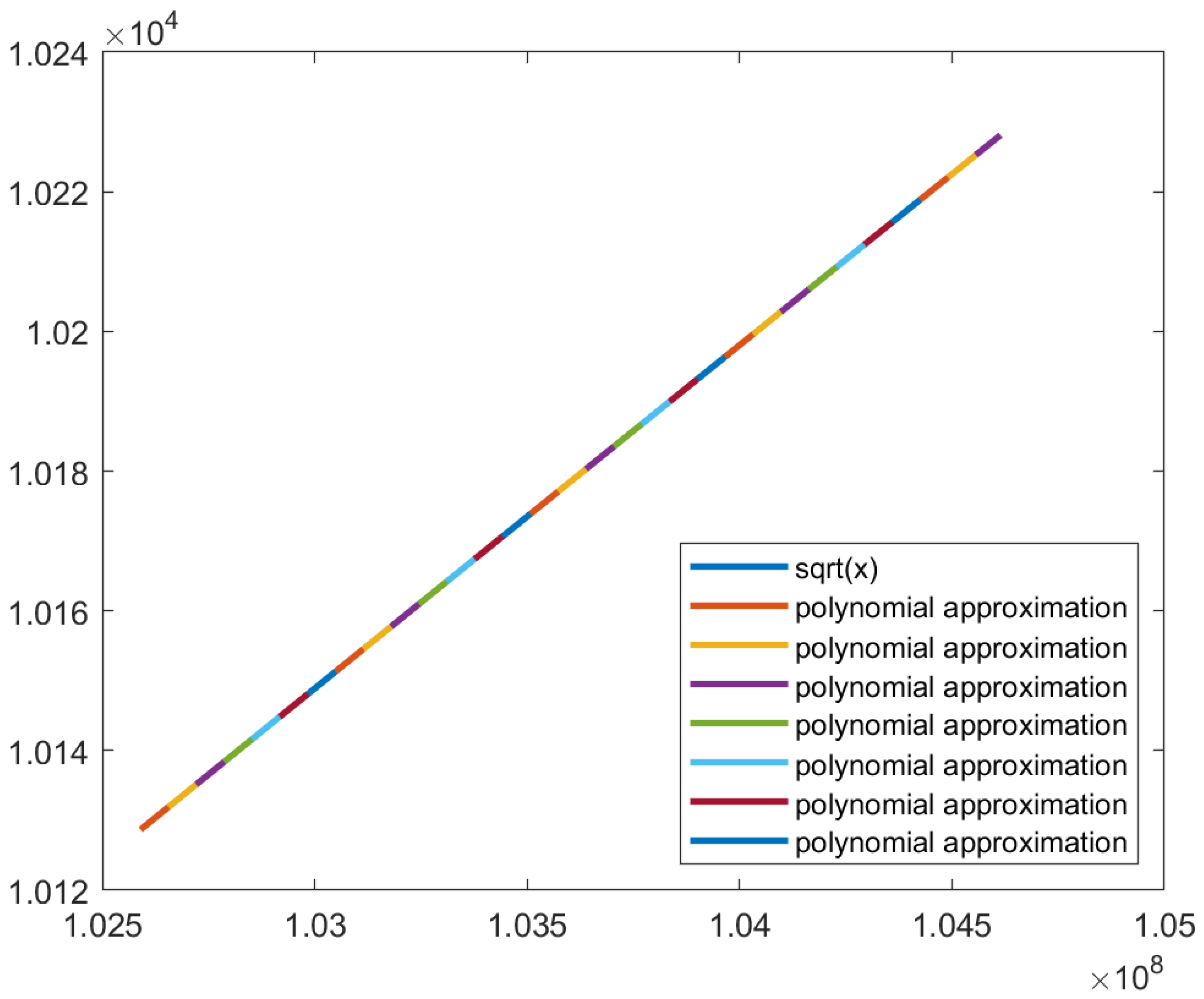Figure 22 shows the image generated using polynomial approximation with the Vandermonde matrix with sixteen subfunctions. The piecewise function is shown in Figure 23. The coefficients for this approximation are shown in Table 6.

5.5. Square root approximation with linear interpolation

The square root function was approximated using linear interpolation with different points spaced by powers of 2. Using polynomial approximation, the lowest number of subfunctions required for an SSIM above 0.99 is 16. For this approximation, the MSE has an order of magnitude of

10^{- 8}

. Therefore, the linear interpolation approximation is expected to have an MSE of the same order.

The MSEs of the square root approximations using linear interpolation with 2 to 990 points are shown in Table 7. This table shows that at least thirty-two points are necessary to satisfy the quality requirements since 17 points have an MSE with an order of magnitude of

10^{- 7}

, lower than the expected

10^{- 8}

. The image generated using the Backprojection algorithm and the 32-point approximation is shown in Figure 24 and has an SSIM of 0.99557. Figure 25 shows the piecewise function.

6. Approximations evaluation

Section 4 and Section 5 presented the development of approximations for the costlier functions of the Backprojection algorithm, namely the square root, sine, and cosine functions. These functions were approximated using linear interpolation and polynomial approximation using the Vandermonde matrix. Furthermore, the sine and cosine functions were approximated using Chebyshev polynomials.

The MSE of the trigonometric approximations and respective SSIM is shown in Table 8. The approximations for the trigonometric functions required a smaller number of terms/subfunctions/points when compared to the square root approximations. Using Chebyshev polynomials, it was possible to obtain an image with an SSIM over 0.99 with an MSE of 3.07750 × 10⁻⁵. The four-term approximation had an SSIM of 1.26110 × 10⁻⁸, concluding that a difference of 3.07624 × 10⁻⁵ in the MSE results in a difference of 5.00000 × 10⁻⁴ in the SSIM. The Chebyshev polynomials approximations are the most precise of the tested approximations. The Chebyshev approximations, however, can only be used for one quadrant. Approximations such as linear interpolation and polynomial approximations using the Vandermonde matrix can be applied to any curve, thus working for every quadrant.

The polynomial approximation using the Vandermonde matrix for the trigonometric functions satisfies the quality requirements using a piecewise function with two subfunctions, both with optimum points and a power of 2 spacing. Therefore, a power of 2 spacing is the best alternative, allowing the identification of the subfunction using the most significant bits of the input. Linear interpolation with a power of 2 spacing requires five points, similar to the polynomial approach. However, linear interpolation requires storing five values, and the line equation is calculated during the computation, while polynomial approximation requires four, and the line equation coefficients are stored in memory.

The square root function approximations presented results similar to the trigonometric approximations. The polynomial approximation using the Vandermonde matrix is more precise than linear interpolation for the same number of lines. Sixteen subfunctions are necessary to obtain an acceptable image using polynomial approximation, while 32 points are necessary for linear interpolation. Therefore, both approximations require the same number of values to be stored in memory. Linear interpolation requires more calculations during the calculation, though.

7. Hardware resource estimates

The approximations developed and described in this paper were implemented in hardware using a high-level synthesis software, Vitis HLS from Xilinx. The hardware resource estimates were obtained from Vitis HLS, considering a Zynq UltraScale+ MPSoC ZCU104 as the target platform.

Table 10 shows the hardware resource usage for the sine and cosine approximations compared to the baseline function. The baseline function is implemented based on the HOTBM method [14]. Every approximation was more efficient and occupied fewer resources than the baseline, from a 35% to 88% reduction in LUTs. The baseline used more FFs, 125, with the approximations using from 34 to 112. Regarding DSPs, the 4-term Chebyshev approximation required the most, 10, with the baseline requiring 8. The other approximations required from 1 to 4. No BRAMs were used in the trigonometric approximations or the baseline function. Both versions, with three and four terms, required no BRAMs. The four-term approximation used 120 DSPs, 42% more when compared to the three-term approximation, 257 LUTs, 19% more, and 60% less DSPs.

The polynomial approximation with the Vandermonde matrix with two subfunctions using optimum points and one quadrant requires 23% more LUTs than the polynomial approximation with a power of 2 spacing, double the DSPs, and 3% more FFs. This is justified by the additional logic to map the input value to the corresponding subfunction, while with a power of 2 spacing, this is done with the most significant bits. Therefore, it is best to use a less precise approximation that facilitates the calculations. With a power of 2 spacing, the quadrant can be selected using the most significant bits of the input angle. This approach is used for the polynomial approximation with the Vandermonde matrix with two subfunctions and the linear interpolation with five points. It is possible to further optimize the circuit by removing additional logic to map the angle to other quadrants and to map the cosine value into the corresponding sine by having larger tables with all quadrants. This optimization results in 75% less LUTs and less 10% FFs.

The linear interpolation approximation shows similar results. First, comparing the linear interpolation approximation to the polynomial approximation shows that linear interpolation requires more hardware resources. 35% more LUTs, 111% less FFs, and one less DSP. A significant reduction is seen when using a larger lookup table for the linear interpolation, using 17 points for the four quadrants instead of only 5 for the first one. This approximation uses 75% less LUTs, 57% less FFs, and one more DSP than the one-quadrant version.

The more resource-efficient approximation is the polynomial approximation with the Vandermonde matrix using a power of 2 spacing and four quadrants. This approximation had an SSIM of 0.99246 and an MSE of 0.000259626 and required 88% less LUTs, 53% less FFs, and 75% less DSPs than the baseline function.

Table 11 shows the hardware resources estimate for each approximation of the square root function approximations. Two approximations were tested: polynomial approximation with Vandermonde matrix using a power of 2 spacing and sixteen subfunctions and linear interpolation with a power of 2 spacing and thirty-two points. As discussed in the previous section, the polynomial approximation requires sixteen subfunctions. That is, saving sixteen slope values and sixteen y-intercept values is necessary, while linear interpolation requires thirty-two points. Both approximations require storing the same number of values, and bits, since the points, slope, and y-intercept values have the same word length of 47 bits. However, while with polynomial approximation, it is only necessary to select the most significant bits to decode which subfunction the input value belongs, with linear interpolation, it is necessary to select the most significant bits to know which points are closest to the input value, plus the slope calculation.

As evidenced by the table, the linear interpolation approximation uses the same number of LUTs as the Polynomial approximation and 5 DSPs, while the polynomial approximation requires one more. The polynomial approximation requires 41 FFs, while linear interpolation requires only 2. However, linear interpolation requires 4 BRAMs.

Compared to the baseline square root function from Vitis HLS, which uses an iterative method, both approximations use less 94% LUTs. The polynomial approximation uses 93% less FFs, and linear interpolation uses 99% less. The baseline function uses no BRAMs or DSPs.

8. Conclusions

This work proposed different approximations for the square root, sine, and cosine functions, the costlier functions of the Backprojection algorithm. For on-board systems with weight, size, and energy requirements, approximations reduce the circuit size and the computation time, increasing the efficiency of the system.

Three approximation methods were tested and proposed in this work: Chebyshev polynomials for the sine and cosine functions, polynomial approximations using the Vandermonde matrix, and linear interpolation for the square root and trigonometric functions. Polynomial approximation and linear interpolation were preferred over traditional square root approximation methods due to the function’s resemblance to a line in the algorithm’s domain. Results showed that the approximations used less 94% LUTs than the baseline function while still meeting the image quality requirements.

The sine and cosine functions were approximated using Chebyshev polynomials, a series-based approximation method that converges faster than the Taylor Series. This method, however, is limited to the first quadrant, requiring additional calculations to map the input angle into this quadrant. Polynomial approximations using the Vandermonde matrix and linear interpolation can be used in every quadrant, removing mapping calculations. The developed approximations, whether for the square root or sine and cosine functions, used fewer resources than the baseline function while still meeting the quality requirements. The polynomial approximation using the Vandermonde matrix was the most efficient approximation, using 88% less LUTs, 53% less FFs, and 75% less DSPs than the baseline function. Evidence shows that it is more efficient to have larger tables with more coefficients and points than smaller tables and additional logic to map the input values to other quadrants.

The proposed approximation methodology can be adapted to other algorithms, requiring a preliminary analysis of the algorithm’s domain and precision requirements. Furthermore, these approximations can be used as redundant computations in fault tolerance mechanisms, such as reduced-precision redundancy, reducing the overhead of the fault tolerance mechanism.

Author Contributions

Conceptualization, R.D. and H.C.; methodology, H.C: and R.D.; software, H.C.; validation, H.C.; formal analysis, H.C.; investigation, H.C., R.D.; resources, H.C., R.D., H.N., J.M., M.V., P.F.; writing—original draft preparation, H.C.; writing—review and editing, H.C., R.D.; supervision, R.D., H.N., J.M., M.V., P.F.; funding acquisition, R.D.

Funding

This research was funded by Fundação para a Ciência e para a Tecnologia grant number UIDB/50021/2020. H.C. would like to thank Fundação para a Ciência e para a Tecnologia for the support through grant SFRH/BD/144133/2019.

Data Availability Statement

This work used and analysed the following publicly available datasets: Gotcha Volumetric SAR Dataset (https://www.sdms.afrl.af.mil/index.php?collection=gotcha, accessed on 1 October 2023) [15].

Conflicts of Interest

The authors declare no conflict of interest. The funders had no role in the design of the study; in the collection, analyses, or interpretation of data; in the writing of the manuscript; or in the decision to publish the results.

Abbreviations

The following abbreviations are used in this manuscript:

BRAM	Block Random Access Memory
DSP	Digital Signal Processor
FF	Flip-Flop
FPGA	Field-Programmable Gate Array
LUT	Lookup Table
MSE	Mean Squared Error
PSNR	Peak Signal-to-Noise Ratio
SAR	Synthetic-Aperture Radar
SNR	Signal-to-Noise Ratio
SSIM	Structural Similarity

References

Cruz, H.; Véstias, M.; Monteiro, J.; Neto, H.; Duarte, R.P. A Review of Synthetic-Aperture Radar Image Formation Algorithms and Implementations: A Computational Perspective. Remote Sensing 2022, 14. Available online: https://www.mdpi.com/2072-4292/14/5/1258. [CrossRef]
Pritsker, D. Efficient Global Back-Projection on an FPGA. 2015 IEEE Radar Conference (RadarCon) 2015, pp. 0204—0209. [CrossRef]
Policarpo Duarte, R.; Cruz, H.; Véstias, M.; Teixeira de Sousa, J.; Neto, H. Hardware Accelerated Backprojection Algorithm on Xilinx UltraScale+ SoC-FPGA for On-Board SAR Image Formation. ESA European Data Handling & Data Processing Conference, Juan-Les-Pins, France 2023.
Gorham, L.A.; Moore, L.J. SAR image formation toolbox for MATLAB. 2010, Vol. 7699, pp. 46 —- 58. [CrossRef]
Wang, Z.; Bovik, A.C.; Sheikh, H.R.; Simoncelli, E.P. Image Quality Assessment: From Error Visibility to Structural Similarity. IEEE Transactions on Image Processing 2004, 13, 600–612. [Google Scholar] [CrossRef] [PubMed]
Pimentel, J.J.; Stillmaker, A.; Bohnenstiehl, B.; Baas, B.M. Area efficient backprojection computation with reduced floating-point word width for SAR image formation. 2015 49th Asilomar Conference on Signals, Systems and Computers 2015, pp. 732—726. [CrossRef]
Barker, K.; Benson, T.; Campbell, D.; Ediger, D.; Gioiosa, R.; Hoisie, A.; Kerbyson, D.; Manzano, J.; Marquez, A.; Song, L.; et al. PERFECT (Power Efficiency Revolution For Embedded Computing Technologies) Benchmark Suite Manual; 2013. http://hpc.pnnl.gov/projects/PERFECT/.
Ganssle, J. The Firmware Handbook; Academic Press, Inc.: Orlando, FL, USA, 2004. [Google Scholar]
Volder, J. The CORDIC Computing Technique. In Proceedings of the Papers Presented at the the March 3-5, 1959, Western Joint Computer Conference, New York, NY, USA, 1959; IRE-AIEE-ACM ’59 (Western), pp. 257–261. [CrossRef]
Hart, J.F. Computer Approximations; Krieger Publishing Co., Inc.: Melbourne, FL, USA, 1978. [Google Scholar]
Stillwell, J. Mathematics and Its History; Springer New York, NY: New York, NY, USA, 2010. [Google Scholar]
Stewart, J. Calculus; Cengage Learning, 2015.
Neto, H.C.; Vestias, M.P. Very low resource table-based FPGA evaluation of elementary functions. In Proceedings of the 2013 International Conference on Reconfigurable Computing and FPGAs (ReConFig), Dec 2013, pp. 1–6. [CrossRef]
Detrey, J.; de Dinechin, F. Floating-Point Trigonometric Functions for FPGAs. In Proceedings of the 2007 International Conference on Field Programmable Logic and Applications, Aug 2007; pp. 29–34. [Google Scholar] [CrossRef]
Jr., C.H.C.; Gorham, L.A.; Minardi, M.J.; Scarborough, S.M.; Naidu, K.D.; Majumder, U.K. A challenge problem for 2D/3D imaging of targets from a volumetric data set in an urban environment. In Proceedings of the Algorithms for Synthetic Aperture Radar Imagery XIV; Zelnio, E.G.; Garber, F.D., Eds. International Society for Optics and Photonics, SPIE, 2007, Vol. 6568, p. 65680. [CrossRef]

Figure 1. Images generated using the Backprojection algorithm and the Gotcha Volumetric SAR dataset, using different word lengths to represent the image variable. Despite the significant difference between the SNR values of the two images, less than 22%, both images are similar to the naked eye and only differ in 0.01 in SSIM.

Figure 2. Function approximation methodology. The square root function is approximated using polynomial approximation using the Vandermonde matrix and linear interpolation, while the sine and cosine functions are approximated using the previous methods as well as Chebyshev polynomials.

Figure 3. Plot of the sine function in the domain

[0, 2 π]

(on top), and plot of the sine function after the variable substitution with the new domain,

[0, 2]

(on the bottom).

Figure 3. Plot of the sine function in the domain

[0, 2 π]

(on top), and plot of the sine function after the variable substitution with the new domain,

[0, 2]

(on the bottom).

Figure 4. Image generated by the Backprojection algorithm using the GOTCHA dataset and the cosine approximation using Chebyshev polynomials with four terms.

Figure 5. Image generated by the Backprojection algorithm using the GOTCHA dataset and the cosine approximation using Chebyshev polynomials with three terms.

Figure 6. Plot of the cosine function (in blue) and the approximation using Chebyshev polynomials with four terms (in red). No differences are observed on this scale.

Figure 7. Plot of the cosine function (in blue) and the approximation using Chebyshev polynomials with three terms (in red). The approximation deviates from the cosine function when x approaches zero.

Figure 8. Polynomial interpolation with the Vandermonde matrix with one function of the sine function in the domain of the Backprojection algorithm using the GOTCHA dataset. The sine function in the first quadrant is in blue, while the approximation is in red.

Figure 9. Image generated using the polynomial approximation with the Vandermonde matrix with one function of the sine function in the domain of the Backprojection algorithm using the GOTCHA dataset.

Figure 10. Polynomial interpolation using the Vandermonde matrix with two subfunctions and optimum points of the sine function in the domain of the Backprojection algorithm using the GOTCHA dataset. The sine function in the first quadrant is blue, the first subfunction is red, and the second subfunction is yellow.

Figure 11. Image generated using the polynomial approximation with the Vandermonde matrix with two subfunctions of the sine function in the domain of the Backprojection algorithm using the GOTCHA dataset.

Figure 12. Plot of the sine function (in blue) and the approximation using polynomial approximation with the Vandermonde matrix (in red).

Figure 13. Image generated using the polynomial approximation with the Vandermonde matrix using two subfunctions approximation of the sine function using the Backprojection algorithm using the GOTCHA dataset.

Figure 14. Polynomial interpolation with the Vandermonde matrix with two subfunctions of the sine function using a power of 2 spacing. The sine curve is in blue, and the piecewise function is in red and yellow.

Figure 15. Image generated using the linear interpolation with five points approximation of the sine function using the Backprojection algorithm using the GOTCHA dataset.

Figure 16. Square root function in the domain of the Backprojection algorithm using the GOTCHA dataset.

Figure 17. Images generated using the Backprojection algorithm and the Gotcha Volumetric SAR dataset, differing in the square root calculation. a) shows the image generated using the square root approximation using polynomial approximation with the Vandermonde matrix, while b) is the baseline image.

Figure 20. Plot of the piecewise function with three functions generated using polynomial approximation with the Vandermonde matrix with optimum points.

Figure 21. Image generated using the Backprojection algorithm using the GOTCHA dataset and the square root approximation using polynomial approximation with the Vandermonde matrix with three subfunctions. This image has an SSIM of 0.95851.

Figure 22. Image generated by the Backprojection algorithm using the GOTCHA dataset and the square root polynomial approximation using the Vandermonde matrix approximation with 16 subfunctions.

Figure 23. Polynomial approximation using the Vandermonde matrix with sixteen subfunctions approximation of the square root function in the domain of the Backprojection algorithm using the GOTCHA dataset.

Figure 24. Image generated by the Backprojection algorithm using the GOTCHA dataset and the square root linear interpolation with thirty-two points.

Figure 25. Linear interpolation with thirty-two point approximation of the square root function in the domain of the Backprojection algorithm using the GOTCHA dataset.

Table 1. SSIM and MSE of the Chebyshev-based approximations with 3 and 4 terms.

Approximation	MSE	SSIM
`cos3820`	1.26110 × 10⁻⁸	0.99595
`cos3820` (3 terms)	3.077 50 × 10⁻⁵	0.99545

Table 2. Polynomial interpolation approximations with different subfunctions and respective MSE for the sine function.

Power of 2	Spacing	Number of subfunctions	MSE
-2	0.250000	2	2.596 26 × 10⁻⁴
-3	0.125000	4	1.644 29 × 10⁻⁵
-4	0.062500	8	1.031 11 × 10⁻⁶
-5	0.031250	16	6.450 20 × 10⁻⁸
-6	0.015625	32	4.032 72 × 10⁻⁹

Table 3. Linear interpolation approximations with different points and respective MSE for the sine function.

Power of 2	Spacing	Number of points	MSE
-1	0.500000	2	2.27638 × 10⁻²
-2	0.250000	3	1.54325 × 10⁻³
-3	0.125000	5	9.84239 × 10⁻⁵
-4	0.062500	9	6.18259 × 10⁻⁶
-5	0.031250	17	3.86894 × 10⁻⁷
-6	0.015625	33	2.41877 × 10⁻⁸

Table 4. SSIM and MSE of the polynomial approximation using the Vandermonde matrix approximation of the square root function with one, two, and three subfunctions.

Number of subfunctions	MSE	SSIM
1	2.31790 × 10⁻³	0.78172
2	7.95870 × 10⁻⁵	0.91314
3	1.61760 × 10⁻⁵	0.95851

Table 5. Polynomial approximations for the square root function and respective MSE, depending on the number of subfunctions and the power-of-2 spacing. The highlighted rows are the best candidates to achieve the quality requirements with fewer resources.

Spacing	Power of 2	Number of subfunctions	MSE
524288	19	4	5.31990 × 10⁻⁶
262144	18	8	3.44260 × 10⁻⁷
131072	17	16	2.24260 × 10⁻⁸
65536	16	31	1.42500 × 10⁻⁹
32768	15	62	8.93150 × 10⁻¹¹
16384	14	124	5.60400 × 10⁻¹²
8192	13	248	3.51000 × 10⁻¹³
4096	12	495	2.20000 × 10⁻¹⁴
2048	11	989	1.00000 × 10⁻¹⁵

Table 6. Slopes and y-intercepts for the line equations of the polynomial approximation piecewise function with sixteen subfunctions for the square root function.

Subfunction	Slope	Y-intercept
1	4.93491 × 10⁻⁵	5065.952890396928
2	4.93176 × 10⁻⁵	5069.186011283943
3	4.92862 × 10⁻⁵	5072.417059076407
4	4.92548 × 10⁻⁵	5075.646050052298
5	4.92235 × 10⁻⁵	5078.872988134498
6	4.91923 × 10⁻⁵	5082.097877234304
7	4.916 11 × 10⁻⁵	5085.320721247944
8	4.91300 × 10⁻⁵	5088.541524063114
9	4.90989 × 10⁻⁵	5091.760289552718
10	4.90679 × 10⁻⁵	5094.977021577670
11	4.90370 × 10⁻⁵	5098.191723986991
12	4.90061 × 10⁻⁵	5101.404400618130
13	4.89753 × 10⁻⁵	5104.615055296567
14	4.89445 × 10⁻⁵	5107.823691833657
15	4.89138 × 10⁻⁵	5111.030314030931
16	4.88917 × 10⁻⁵	5113.343963108114

Table 7. Linear interpolation approximations for the square root function and respective MSE, depending on the number of subfunctions and the power-of-2 spacing.

Power of 2	Spacing	Number of points	MSE
21	2097152	2	9.05081 × 10⁻³
20	1048576	3	4.98988 × 10⁻⁴
19	524288	5	3.19193 × 10⁻⁵
18	262144	9	2.06555 × 10⁻⁶
17	131072	17	1.34554 × 10⁻⁷
16	65536	32	8.54979 × 10⁻⁹
15	32768	63	5.35875 × 10⁻¹⁰
14	16384	125	3.36220 × 10⁻¹¹
13	8192	249	2.10900 × 10⁻¹²
12	4096	496	1.32000 × 10⁻¹³
11	2048	989	8.00000 × 10⁻¹⁵

Table 8. Comparison between the Chebyshev polynomials, polynomial approximation with the Vandermonde matrix using optimal points, power of 2 spacing, and linear interpolation approximations with power of 2 spacing for the trigonometric functions. The highlighted rows indicate the minimum number of functions necessary to obtain an SSIM over 0.99.

Approximation	Number of terms/subfunctions/points	MSE	SSIM
Chebyshev polynomials	4	1.26110 × 10⁻⁸	0.99595
Chebyshev polynomials	3	3.07750 × 10⁻⁵	0.99545
Polynomial approximation with Vandermonde matrix (optimum points)	1	3.94020 × 10⁻³	0.95962
	2	2.06271 × 10⁻⁴	0.99314
Polynomial approximation with Vandermonde matrix (power of 2 spacing)	1	3.93980 × 10⁻³	NA
	2	2.59626 × 10⁻⁴	0.99246
	4	1.64429 × 10⁻⁵	NA
	8	1.03111 × 10⁻⁶	NA
	16	6.45020 × 10⁻⁸	NA
	32	4.03272 × 10⁻⁹	NA
Linear interpolation (power of 2 spacing)	2	2.27638 × 10⁻²	NA
	3	1.54325 × 10⁻³	NA
	5	9.84239 × 10⁻⁵	0.99562
	9	6.18259 × 10⁻⁶	NA
	17	3.86894 × 10⁻⁷	NA
	33	2.41877 × 10⁻⁸	NA

Table 9. Comparison between the polynomial approximation with the Vandermonde matrix using optimal points, power of 2 spacing, and linear interpolation with power of 2 spacing approximations for the square root function. The highlighted rows indicate the minimum number of functions necessary to obtain an SSIM over 0.99.

Approximation	Number of subfunctions/points	MSE	SSIM
Polynomial approximation with Vandermonde matrix (optimal points)	1	1.50845 × 10⁻³	0.78172
	2	7.95871 × 10⁻⁵	0.91314
	3	1.61760 × 10⁻⁵	0.95851
Polynomial approximation with Vandermonde matrix (power of 2 spacing)	4	5.31990 × 10⁻⁶	NA
	8	3.44260 × 10⁻⁷	0.98916
	16	2.24260 × 10⁻⁸	0.99436
	31	1.42500 × 10⁻⁹	NA
	62	8.93150 × 10⁻¹⁰	NA
	124	5.60400 × 10⁻¹¹	NA
	248	3.51000 × 10⁻¹³	NA
	495	2.20000 × 10⁻¹⁴	NA
	989	1.00000 × 10⁻¹⁵	NA
Linear interpolation (power of 2 spacing)	2	9.05081 × 10⁻³	NA
	3	4.98988 × 10⁻⁴	NA
	5	3.19193 × 10⁻⁵	NA
	9	2.06555 × 10⁻⁶	NA
	17	1.34554 × 10⁻⁷	NA
	32	8.54979 × 10⁻⁹	0.99557
	63	5.35875 × 10⁻¹⁰	NA
	125	3.36220 × 10⁻¹¹	NA
	249	2.10900 × 10⁻¹²	NA
	496	1.32000 × 10⁻¹³	NA
	990	8.00000 × 10⁻¹⁵	NA

Table 10. Hardware resources usage of the Chebyshev polynomials, polynomial approximation with the Vandermonde matrix, and linear interpolation approximations for the sine and cosine functions.

Approximation	Number of terms/ subfunctions/ points	Hardware resources
Approximation	Number of terms/ subfunctions/ points	BRAMs	DSPs	FFs	LUTs
Baseline sine and cosine (from hls_math.h, using the HOTBM method [14])	–	0	8	125	504
Chebyshev polynomials	4	0	10	34	257
Chebyshev polynomials	3	0	7	87	206
Polynomial approximation with the Vandermonde matrix (optimum points and one quadrant)	2	0	4	61	297
Polynomial approximation with the Vandermonde matrix (power of 2 spacing and one quadrant)	2	0	2	59	241
Polynomial approximation with the Vandermonde matrix (power of 2 spacing (and four quadrants)	8	0	2	53	59
Linear interpolation (power of 2 spacing and one quadrant)	5	0	1	112	326
Linear interpolation (power of 2 spacing and four quadrants)	17	0	2	48	81
Device total	–	624	1728	460800	230400

Table 11. Hardware resources usage of the baseline square root implementation from Vitis HLS, Chebyshev polynomials, polynomial approximation with the Vandermonde matrix, and linear interpolation approximations for the square root function.

Approximation	Number of subfunctions/points	Hardware Resources
Approximation	Number of subfunctions/points	BRAMs	DSPs	FFs	LUTs
Baseline square root (from hls_math.h)	–	0	0	680	2759
Polynomial approximation with Vandermonde matrix (power of 2 spacing)	16	0	6	41	165
Linear interpolation (power of 2 spacing)	32	4	5	2	165
Device total	–	624	1728	460800	230400

Disclaimer/Publisher’s Note: The statements, opinions and data contained in all publications are solely those of the individual author(s) and contributor(s) and not of MDPI and/or the editor(s). MDPI and/or the editor(s) disclaim responsibility for any injury to people or property resulting from any ideas, methods, instructions or products referred to in the content.

© 2023 by the authors. Licensee MDPI, Basel, Switzerland. This article is an open access article distributed under the terms and conditions of the Creative Commons Attribution (CC BY) license (http://creativecommons.org/licenses/by/4.0/).

Copyright: This open access article is published under a Creative Commons CC BY 4.0 license, which permit the free download, distribution, and reuse, provided that the author and preprint are cited in any reuse.

MDPI Initiatives

Important Links

Choose an area of interest and we will send you notifications of new preprints at your preferred frequency.

Disclaimer

Algorithm-Specific Optimizations for On-Board Real-Time Backprojection on FPGA

Abstract

1. Introduction

2. Background and related work

2.1. Backprojection algorithm

2.2. Image quality metrics

3. Approximation methodology

4. Trigonometric approximations

4.1. Modifications to the Backprojection algorithm

4.2. Chebyshev polynomials and Bessel functions approximation

4.3. Sine approximation using polynomial approximation using the Vandermonde matrix approximation

4.3.1. Sine approximation using polynomial approximation using the Vandermonde matrix and subfunctions with optimum points

4.3.2. Sine approximation using polynomial approximation using the Vandermonde matrix and subfunctions with a power of 2 spacing

4.4. Sine approximation using linear interpolation with power of 2 spacing

5. Square root approximation

5.1. Square root approximation with polynomial approximation using the Vandermonde matrix

5.2. Polynomial approximation using the Vandermonde matrix with subfunctions using optimum points

5.3. Second-degree polynomial approximation using the Vandermonde matrix with subfunctions using power of 2 spacing

5.4. Polynomial approximation using the Vandermonde matrix with subfunctions using power of 2 spacing

5.5. Square root approximation with linear interpolation

6. Approximations evaluation

7. Hardware resource estimates

8. Conclusions

Author Contributions

Funding

Data Availability Statement

Conflicts of Interest

Abbreviations

References

MDPI Initiatives

Important Links

Subscribe