Submitted:
09 December 2023
Posted:
11 December 2023
You are already at the latest version
Abstract
Keywords:
1. Introduction
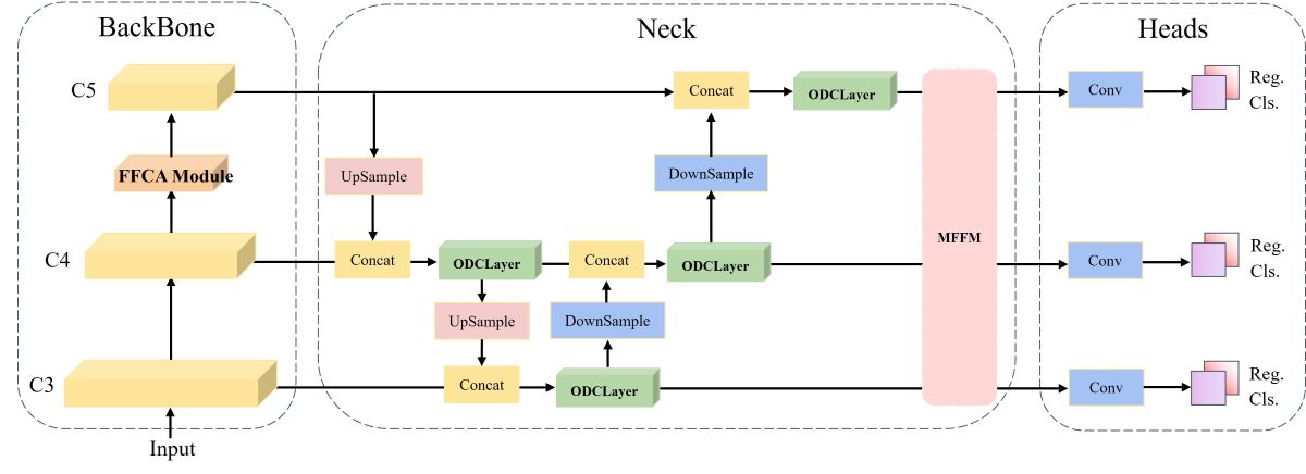
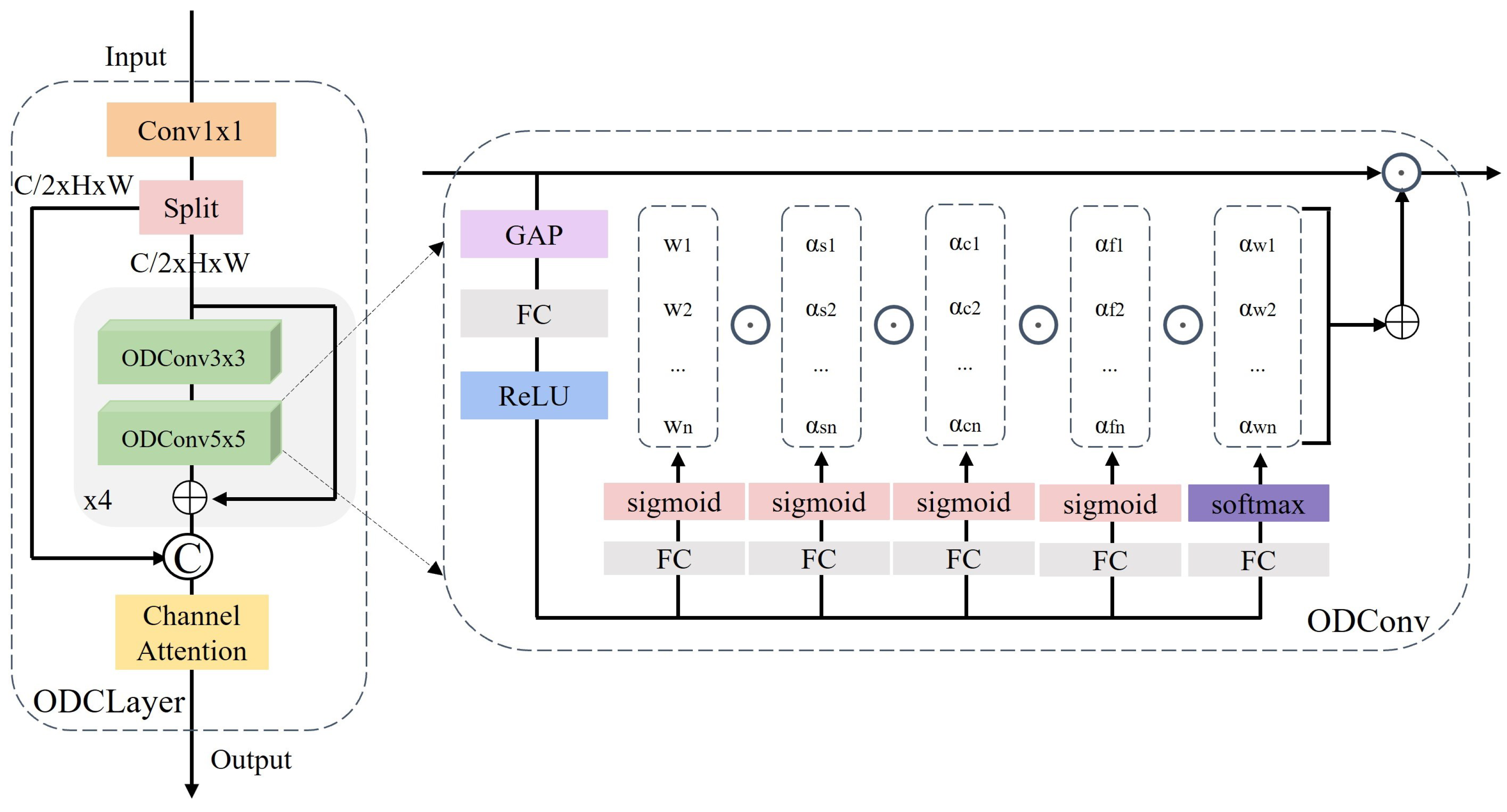
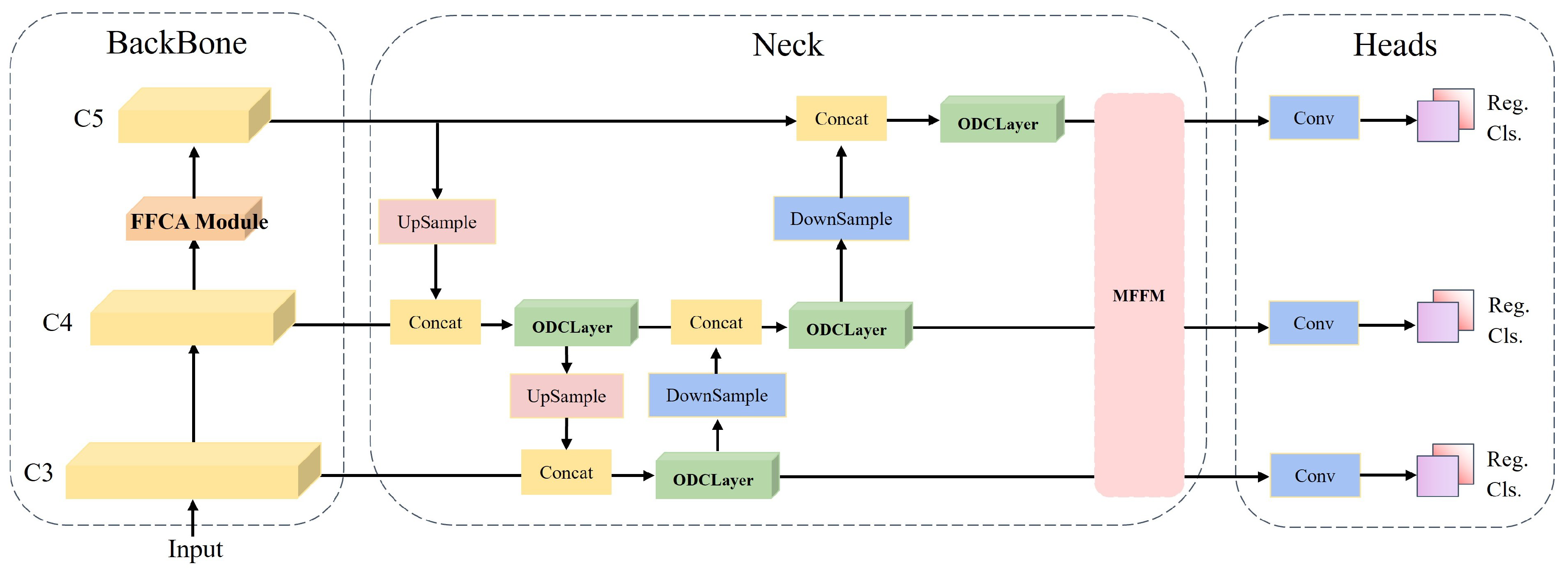
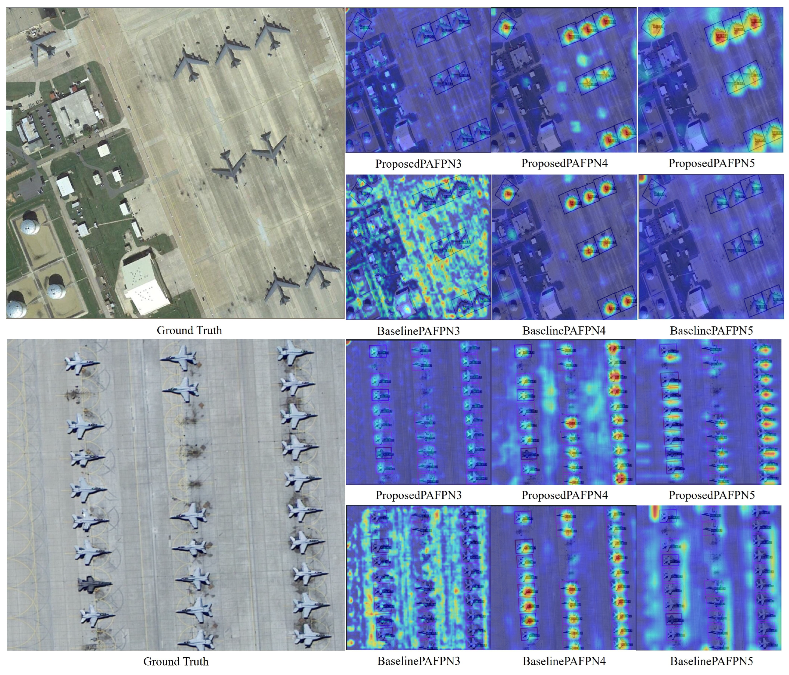
- In the backbone network, we utilize a multi-level feature fusion mechanism to acquire features of different scales. Subsequently, context information is selectively extracted from local to global levels at varying granularities, resulting in feature maps equal in size to the input features. Finally, these feature maps are injected into the original features to obtain relevant information about the objects of interest without altering their size.
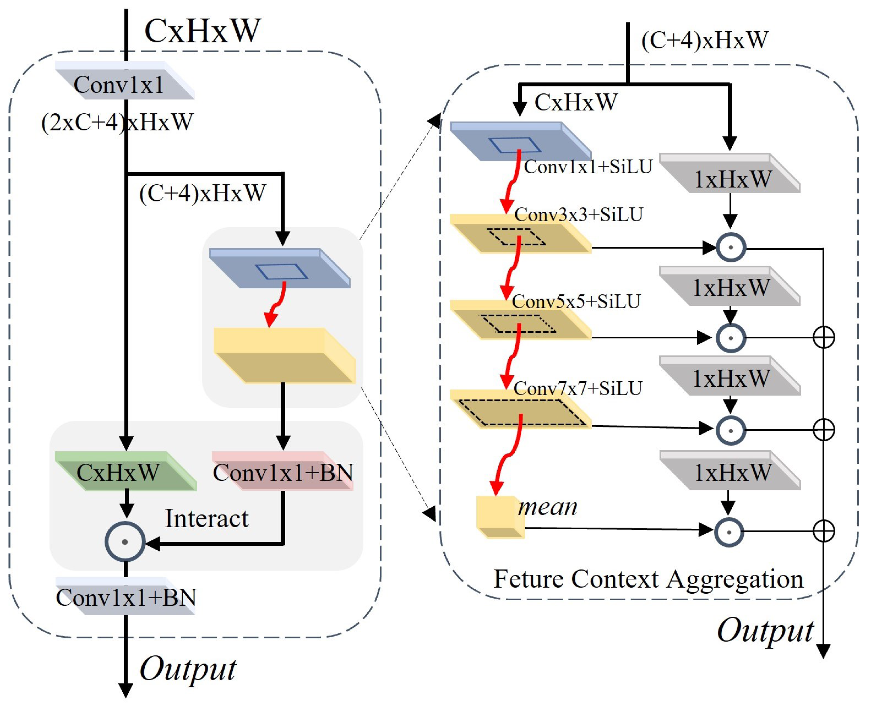
- We design a feature aggregation module that assigns varying attention across multiple dimensions to the fused feature map information, thereby improving performance in capturing rich contextual information and consequently enhancing pixel-level attention towards objects of interest.
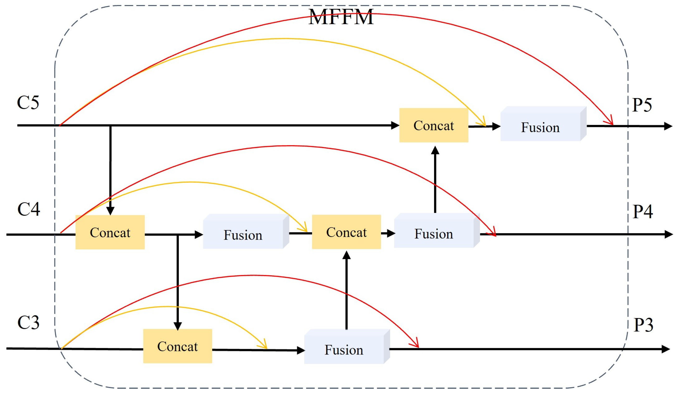
- Within the feature pyramid, we efficiently harness original feature information to process multi-scale features more effectively by introducing a multi-scale fusion pyramid network. This network connects original features and fused features while shortening the information transmission paths, extending from large-scale features to fused small-scale features, and enabling the module to optimally utilize features at each stage.
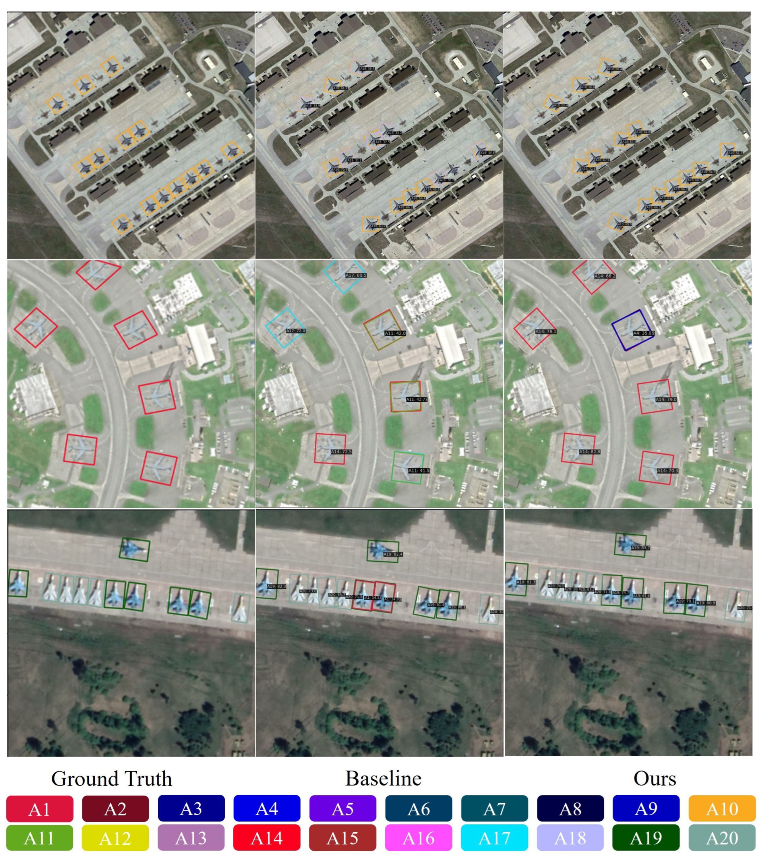
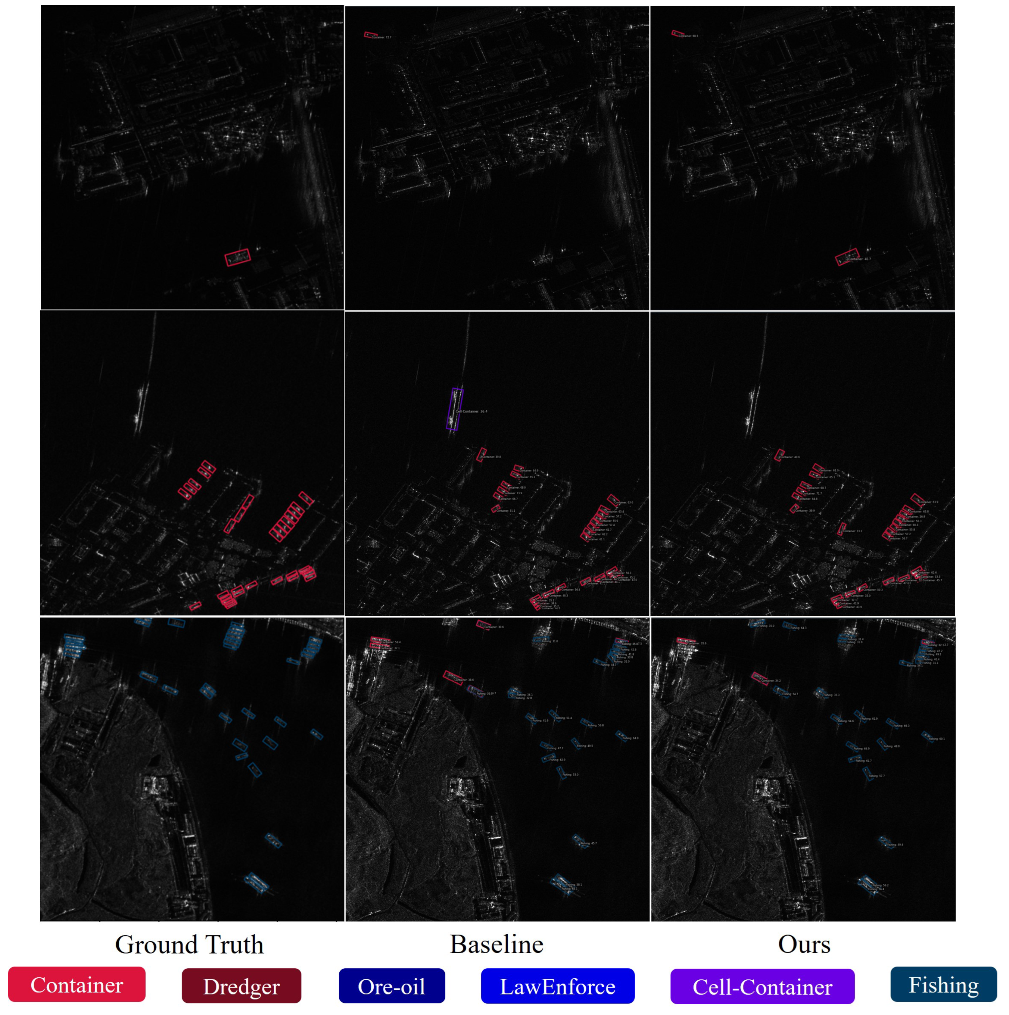
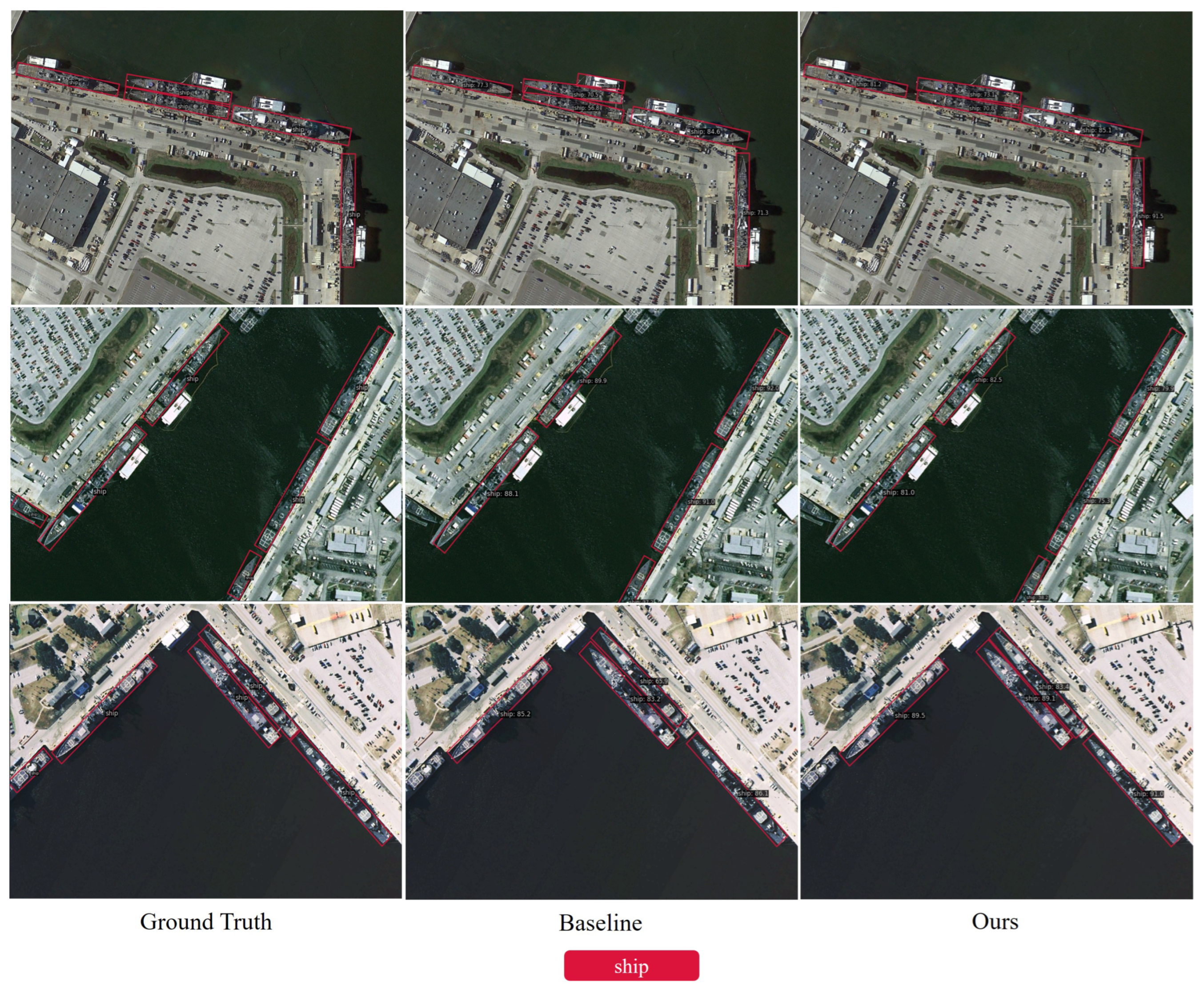
- We introduce a novel object network and conduct extensive experiments on three challenging datasets: MAR20, SRSDD, and HRSC, affirming the effectiveness of our approach. The experimental results demonstrate outstanding performance.
2. Releated Work
2.1. Object Detection in General Scenarios
2.2. Object Detection in Remote Sensing Scenarios
3. Methodology
3.1. Basic Rotated Detection Method as Baseline
3.2. Focused Feature Context Aggregation Module
3.3. Multiscale Feature Fusion Module
3.4. Feature Context Information Enhancement Module
3.5. MFCANet
4. Experiments
4.1. Datasets and Evaluation Metrics
4.1.1. Datasets
4.1.2. Evaluation Metrics
4.2. Implementation details
4.3. Comparisons with SOTA
4.3.1. Results on MAR20
4.3.2. Results on SRSDD
4.3.3. Results on HRSC
4.4. Ablation Study
4.4.1. Ablation study with different feature fusion methods in MFFM
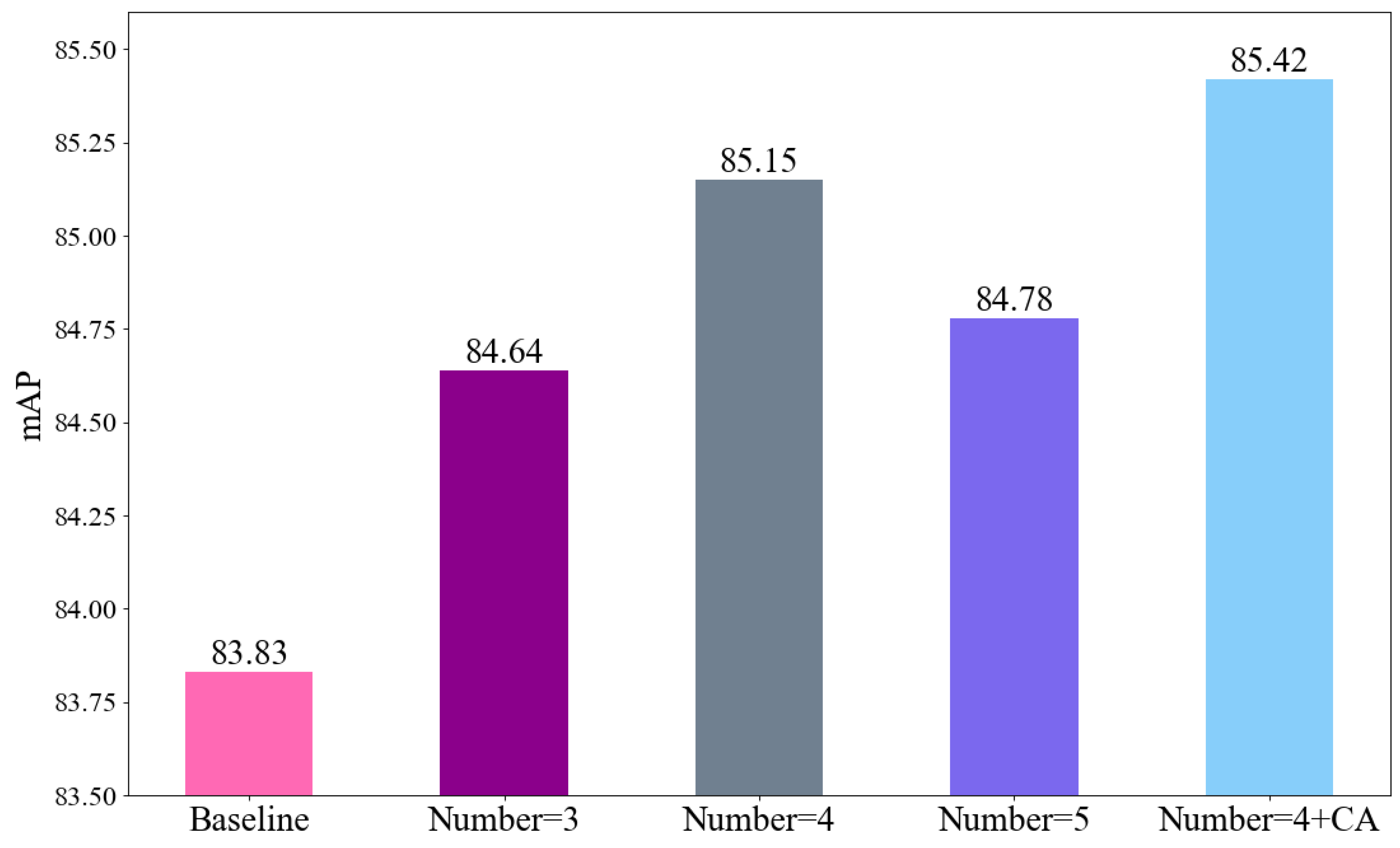
4.4.2. Ablation study on ODCLayer modules.
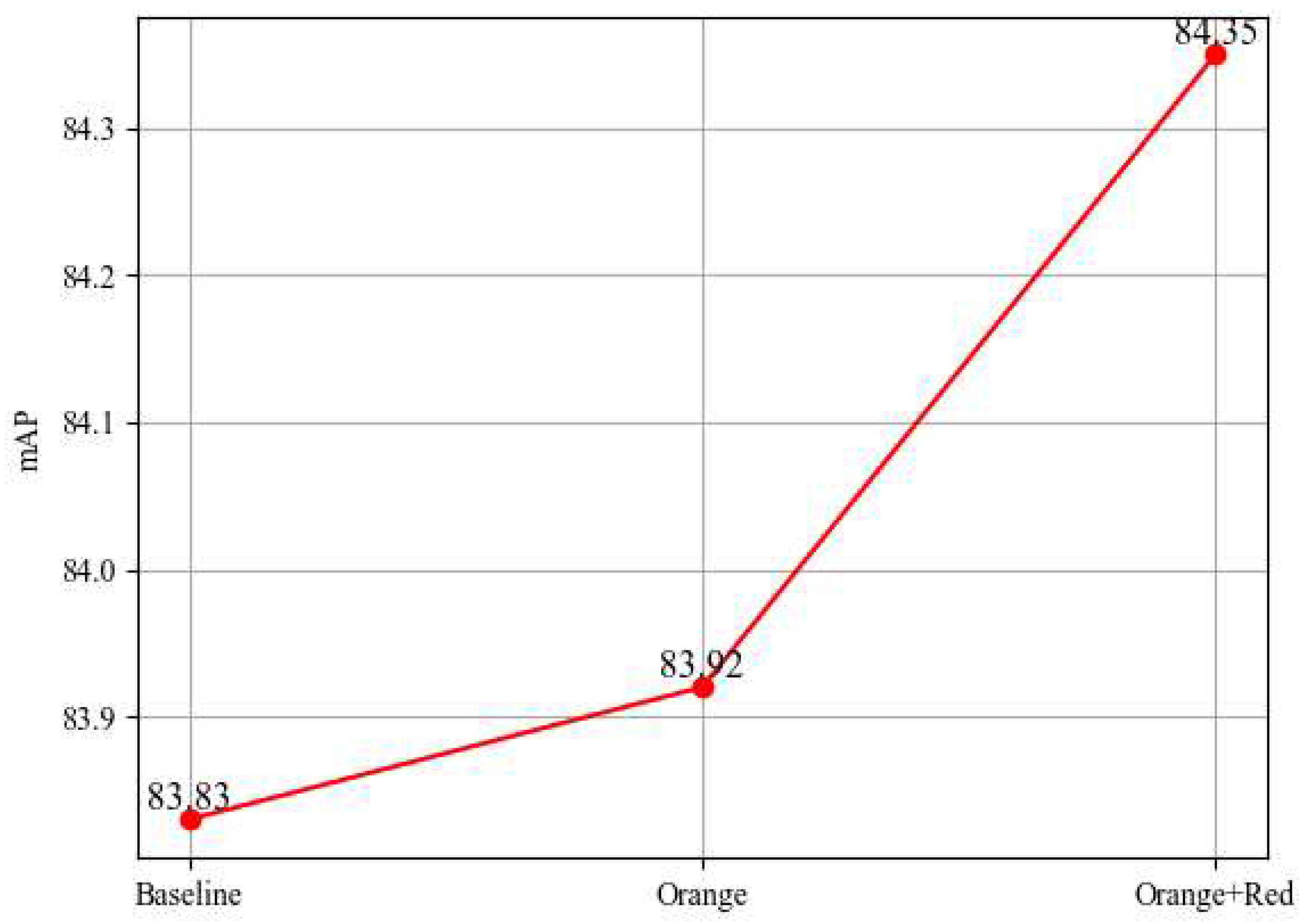
4.4.3. Ablation study on MFCANet
5. Conclusion
Author Contributions
Funding
References
- Barmpoutis, P.; Papaioannou, P.; Dimitropoulos, K.; Grammalidis, N. A review on early forest fire detection systems using optical remote sensing. Sensors 2020, 20, 6442. [CrossRef]
- Mohan, A.; Singh, A.K.; Kumar, B.; Dwivedi, R. Review on remote sensing methods for landslide detection using machine and deep learning. Transactions on Emerging Telecommunications Technologies 2021, 32(7), e3998. [CrossRef]
- Hu, J.; Huang, Z.; Shen, F.; He, D.; Xian, Q. A Robust Method for Roof Extraction and Height Estimation. In IGARSS 2023-2023 IEEE International Geoscience and Remote Sensing Symposium; IEEE: 2023.
- Weng, W.; Ling, W.; Lin, F.; Ren, J.; Shen, F. A Novel Cross Frequency-domain Interaction Learning for Aerial Oriented Object Detection. In Chinese Conference on Pattern Recognition and Computer Vision (PRCV); Springer: 2023.
- LI, B.; XIE, X.; WEI, X.; TANG, W. Ship detection and classification from optical remote sensing images: A survey. Chinese Journal of Aeronautics 2021, 34(3), 145–163. [CrossRef]
- Girshick, R.; Donahue, J.; Darrell, T.; Malik, J. Rich feature hierarchies for accurate object detection and semantic segmentation. In Proceedings of the IEEE conference on computer vision and pattern recognition; 2014; pp. 580–587.
- Girshick, R. Fast r-cnn. In Proceedings of the IEEE international conference on computer vision; 2015; pp. 1440–1448.
- Ren, S.; He, K.; Girshick, R.; Sun, J. Faster r-cnn: Towards real-time object detection with region proposal networks. Advances in neural information processing systems 2015, 28.
- Dai, J.; Li, Y.; He, K.; Sun, J. R-fcn: Object detection via region-based fully convolutional networks. Advances in neural information processing systems 2016, 29.
- Redmon, J.; Farhadi, A. Yolov3: An incremental improvement. arXiv preprint arXiv:1804.02767 2018.
- Bochkovskiy, A.; Wang, C.-Y.; Liao, H.-Y.M. YOLOv4: Optimal speed and accuracy of object detection. arXiv preprint arXiv:2004.10934 2020.
- Zhu, X.; Lyu, S.; Wang, X.; Zhao, Q. TPH-YOLOv5: Improved YOLOv5 based on transformer prediction head for object detection on drone-captured scenarios. In Proceedings of the IEEE/CVF international conference on computer vision; 2021; pp. 2778–2788. [CrossRef]
- Li, C.; Li, L.; Jiang, H.; Weng, K.; Geng, Y.; Li, L.; Ke, Z.; Li, Q.; Cheng, M.; Nie, W.; others. YOLOv6: A single-stage object detection framework for industrial applications. arXiv preprint arXiv:2209.02976 2022.
- Wang, C.-Y.; Bochkovskiy, A.; Liao, H.-Y.M. YOLOv7: Trainable bag-of-freebies sets new state-of-the-art for real-time object detectors. In Proceedings of the IEEE/CVF Conference on Computer Vision and Pattern Recognition; 2023; pp. 7464–7475.
- Shen, F.; Ye, H.; Zhang, J.; Wang, C.; Han, X.; Yang, W. Advancing Pose-Guided Image Synthesis with Progressive Conditional Diffusion Models. arXiv preprint arXiv:2310.06313 2023.
- Shen, F.; He, X.; Wei, M.; Xie, Y. A competitive method to vipriors object detection challenge. arXiv preprint arXiv:2104.09059 2021.
- Han, J.; Ding, J.; Li, J.; Xia, G.-S. Align deep features for oriented object detection. IEEE Transactions on Geoscience and Remote Sensing 2021, 60, 1–11.
- Lyu, C.; Zhang, W.; Huang, H.; Zhou, Y.; Wang, Y.; Liu, Y.; Zhang, S.; Chen, K. Rtmdet: An empirical study of designing real-time object detectors. arXiv preprint arXiv:2212.07784 2022.
- Lin, T.-Y.; Dollár, P.; Girshick, R.; He, K.; Hariharan, B.; Belongie, S. Feature pyramid networks for object detection. In Proceedings of the IEEE conference on computer vision and pattern recognition; 2017; pp. 2117–2125.
- Liu, S.; Qi, L.; Qin, H.; Shi, J.; Jia, J. Path aggregation network for instance segmentation. In Proceedings of the IEEE conference on computer vision and pattern recognition; 2018; pp. 8759–8768.
- Zheng, S.; Wu, Z.; Xu, Y.; Wei, Z. Instance-Aware Spatial-Frequency Feature Fusion Detector for Oriented Object Detection in Remote Sensing Images. IEEE Transactions on Geoscience and Remote Sensing 2023. [CrossRef]
- Zheng, S.; Wu, Z.; Xu, Y.; Wei, Z.; Plaza, A. Learning orientation information from frequency-domain for oriented object detection in remote sensing images. IEEE Transactions on Geoscience and Remote Sensing 2022, 60, 1–12. [CrossRef]
- Chen, S.; Zhao, J.; Zhou, Y.; Wang, H.; Yao, R.; Zhang, L.; Xue, Y. Info-FPN: An Informative Feature Pyramid Network for object detection in remote sensing images. Expert Systems with Applications 2023, 214, 119132. [CrossRef]
- Zhang, G.; Lu, S.; Zhang, W. CAD-Net: A context-aware detection network for objects in remote sensing imagery. IEEE Transactions on Geoscience and Remote Sensing 2019, 57(12), 10015–10024.
- LI, Y.; WANG, H.; FANG, Y.; WANG, S.; LI, Z.; JIANG, B. Learning power Gaussian modeling loss for dense rotated object detection in remote sensing images. Chinese Journal of Aeronautics 2023, Elsevier. [CrossRef]
- Zhang, W.; Jiao, L.; Li, Y.; Huang, Z.; Wang, H. Laplacian feature pyramid network for object detection in VHR optical remote sensing images. IEEE Transactions on Geoscience and Remote Sensing 2021, 60, 1–14. [CrossRef]
- Li, Y.; Wang, H.; Dang, L.M.; Song, H-K.; Moon, H. ORCNN-X: Attention-Driven Multiscale Network for Detecting Small Objects in Complex Aerial Scenes. Remote Sensing 2023, 15(14), 3497. [CrossRef]
- Chen, J.; Hong, H.; Song, B.; Guo, J.; Chen, C.; Xu, J. MDCT: Multi-Kernel Dilated Convolution and Transformer for One-Stage Object Detection of Remote Sensing Images. Remote Sensing 2023, 15(2), 371. [CrossRef]
- Shen, F.; Xie, Y.; Zhu, J.; Zhu, X.; Zeng, H. Git: Graph interactive transformer for vehicle re-identification. IEEE Transactions on Image Processing 2023. [CrossRef]
- Shen, F.; Peng, X.; Wang, L.; Zhang, X.; Shu, M.; Wang, Y. HSGM: A Hierarchical Similarity Graph Module for Object Re-identification. In 2022 IEEE International Conference on Multimedia and Expo; 2022.
- Shen, F.; Shu, X.; Du, X.; Tang, J. Pedestrian-specific Bipartite-aware Similarity Learning for Text-based Person Retrieval. In Proceedings of the 31th ACM International Conference on Multimedia; 2023.
- Wang, Q.; Wu, B.; Zhu, P.; Li, P.; Zuo, W.; Hu, Q. ECA-Net: Efficient channel attention for deep convolutional neural networks. In Proceedings of the IEEE/CVF conference on computer vision and pattern recognition; 2020; pp. 11534–11542.
- Zhang, Q.-L.; Yang, Y.-B. Sa-net: Shuffle attention for deep convolutional neural networks. In ICASSP 2021-2021 IEEE International Conference on Acoustics, Speech and Signal Processing (ICASSP); 2021; pp. 2235–2239. [CrossRef]
- Lee, Y.; Park, J. Centermask: Real-time anchor-free instance segmentation. In Proceedings of the IEEE/CVF conference on computer vision and pattern recognition; 2020; pp. 13906–13915.
- Dosovitskiy, A.; Beyer, L.; Kolesnikov, A.; Weissenborn, D.; Zhai, X.; Unterthiner, T.; Dehghani, M.; Minderer, M.; Heigold, G.; Gelly, S.; others. An image is worth 16x16 words: Transformers for image recognition at scale. arXiv preprint arXiv:2010.11929 2020.
- Hu, J.; Huang, Z.; Shen, F.; He, D.; Xian, Q. A Bag of Tricks for Fine-Grained roof Extraction. In IGARSS 2023-2023 IEEE International Geoscience and Remote Sensing Symposium; 2023.
- Liu, Z.; Lin, Y.; Cao, Y.; Hu, H.; Wei, Y.; Zhang, Z.; Lin, S.; Guo, B. Swin transformer: Hierarchical vision transformer using shifted windows. In Proceedings of the IEEE/CVF international conference on computer vision; 2021; pp. 10012–10022.
- Wu, H.; Shen, F.; Zhu, J.; Zeng, H.; Zhu, X.; Lei, Z. A sample-proxy dual triplet loss function for object re-identification. IET Image Processing 2022, 16(14), 3781–3789.
- Zhang, J.; Lei, J.; Xie, W.; Fang, Z.; Li, Y.; Du, Q. SuperYOLO: Super resolution assisted object detection in multimodal remote sensing imagery. IEEE Transactions on Geoscience and Remote Sensing 2023, 61, 1–15. [CrossRef]
- Qiao, C.; Shen, F.; Wang, X.; Wang, R.; Cao, F.; Zhao, S.; Li, C. A Novel Multi-Frequency Coordinated Module for SAR Ship Detection. In 2022 IEEE 34th International Conference on Tools with Artificial Intelligence (ICTAI); 2022; pp. 804–811.
- Shen, F.; Wei, M.; Ren, J. HSGNet: Object Re-identification with Hierarchical Similarity Graph Network. arXiv preprint arXiv:2211.05486 2022.
- Liu, F.; Chen, R.; Zhang, J.; Ding, S.; Liu, H.; Ma, S.; Xing, K. ESRTMDet: An End-to-End Super-Resolution Enhanced Real-Time Rotated Object Detector for Degraded Aerial Images. IEEE Journal of Selected Topics in Applied Earth Observations and Remote Sensing 2023, IEEE. [CrossRef]
- Shen, F.; Zhu, J.; Zhu, X.; Xie, Y.; Huang, J. Exploring spatial significance via hybrid pyramidal graph network for vehicle re-identification. IEEE Transactions on Intelligent Transportation Systems 2021, 23(7), 8793–8804. [CrossRef]
- Min, L.; Fan, Z.; Lv, Q.; Reda, M.; Shen, L.; Wang, B. YOLO-DCTI: Small Object Detection in Remote Sensing Base on Contextual Transformer Enhancement. Remote Sensing 2023, 15(16), 3970. [CrossRef]
- Cheng, G.; Wang, J.; Li, K.; Xie, X.; Lang, C.; Yao, Y.; Han, J. Anchor-free oriented proposal generator for object detection. IEEE Transactions on Geoscience and Remote Sensing 2022, 60, 1–11. [CrossRef]
- Tian, Z.; Shen, C.; Chen, H.; He, T. FCOS: A simple and strong anchor-free object detector. IEEE Transactions on Pattern Analysis and Machine Intelligence 2020, 44(4), 1922–1933.
- Wang, X.; Girdhar, R.; Yu, S. X.; Misra, I. Cut and learn for unsupervised object detection and instance segmentation. In Proceedings of the IEEE/CVF Conference on Computer Vision and Pattern Recognition; 2023; pp. 3124–3134.
- Yang, X.; Zhang, G.; Li, W.; Wang, X.; Zhou, Y.; Yan, J. H2RBox: Horizonal Box Annotation is All You Need for Oriented Object Detection. arXiv preprint arXiv:2210.06742 2022.
- Sun, X.; Cheng, G.; Pei, L.; Li, H.; Han, J. Threatening patch attacks on object detection in optical remote sensing images. IEEE Transactions on Geoscience and Remote Sensing 2023, IEEE. [CrossRef]
- Wan, D.; Lu, R.; Wang, S.; Shen, S.; Xu, T.; Lang, X. YOLO-HR: Improved YOLOv5 for Object Detection in High-Resolution Optical Remote Sensing Images. Remote Sensing 2023, 15(3), 614. [CrossRef]
- Yang, X.; Yan, J.; Ming, Q.; Wang, W.; Zhang, X.; Tian, Q. Rethinking rotated object detection with gaussian wasserstein distance loss. In International conference on machine learning; 2021; pp. 11830–11841.
- Ge, Z.; Liu, S.; Wang, F.; Li, Z.; Sun, J. Yolox: Exceeding yolo series in 2021. arXiv preprint arXiv:2107.08430 2021.
- Liu, Z.; Mao, H.; Wu, C.-Y.; Feichtenhofer, C.; Darrell, T.; Xie, S. A convnet for the 2020s. In Proceedings of the IEEE/CVF conference on computer vision and pattern recognition; 2022; pp. 11976–11986.
- Ding, X.; Zhang, X.; Han, J.; Ding, G. Scaling up your kernels to 31x31: Revisiting large kernel design in cnns. In Proceedings of the IEEE/CVF conference on computer vision and pattern recognition; 2022; pp. 11963–11975.
- Wang, X.; Girshick, R.; Gupta, A.; He, K. Non-local neural networks. In Proceedings of the IEEE conference on computer vision and pattern recognition; 2018; pp. 7794–7803.
- Zhou, Y.; Yang, X.; Zhang, G.; Wang, J.; Liu, Y.; Hou, L.; Jiang, X.; Liu, X.; Yan, J.; Lyu, C. Mmrotate: A rotated object detection benchmark using pytorch. In Proceedings of the 30th ACM International Conference on Multimedia; 2022; pp. 7331–7334.
- Qian, X.; Zhang, N.; Wang, W. Smooth giou loss for oriented object detection in remote sensing images. Remote Sensing 2023, 15(5), 1259. [CrossRef]
- Zhang, Y.; Wang, Y.; Zhang, N.; Li, Z.; Zhao, Z.; Gao, Y.; Chen, C.; Feng, H. RoI Fusion Strategy with Self-Attention Mechanism for Object Detection in Remote Sensing Images. IEEE Journal of Selected Topics in Applied Earth Observations and Remote Sensing 2023, IEEE. [CrossRef]
- Ding, J.; Xue, N.; Long, Y.; Xia, G.; Lu, Q. Learning RoI transformer for oriented object detection in aerial images. In Proceedings of the IEEE/CVF Conference on Computer Vision and Pattern Recognition; 2019; pp. 2849–2858.
- Yang, X.; Yan, J.; Feng, Z.; He, T. R3det: Refined single-stage detector with feature refinement for rotating object. Proceedings of the AAAI conference on artificial intelligence 2021, 35(4), 3163–3171. [CrossRef]
- Han, J.; Ding, J.; Li, J.; Xia, G. Align deep features for oriented object detection. IEEE Transactions on Geoscience and Remote Sensing 2021, 60, 1–11.
- Chen, W.; Han, B.; Yang, Z.; Gao, X. MSSDet: Multi-Scale Ship-Detection Framework in Optical Remote-Sensing Images and New Benchmark. Remote Sensing 2022, 14(21), 5460. [CrossRef]
- Xie, X.; Cheng, G.; Wang, J.; Yao, X.; Han, J. Oriented R-CNN for object detection. In Proceedings of the IEEE/CVF international conference on computer vision; 2021; pp. 3520–3529.
- Yu, W.; Cheng, G.; Wang, M.; Yao, Y.; Xie, X.; Yao, XW.; Han, JW. MAR20: A Benchmark for Military Aircraft Recognition in Remote Sensing Images. National Remote Sensing Bulletin 2022. [CrossRef]
- Liu, Z.; Yuan, L.; Weng, L.; Yang, Y. A high resolution optical satellite image dataset for ship recognition and some new baselines. In International conference on pattern recognition applications and methods; 2017; Volume 2; pp. 324–331.
- Li, K.; Wan, G.; Cheng, G.; Meng, L.; Han, J. Object detection in optical remote sensing images: A survey and a new benchmark. ISPRS journal of photogrammetry and remote sensing 2020, 159, 296–307.
- Shen, F.; Du, X.; Zhang, L.; Tang, J. Triplet Contrastive Learning for Unsupervised Vehicle Re-identification. arXiv preprint arXiv:2301.09498 2023.
- Wang, Z.; Bao, C.; Cao, J.; Hao, Q. AOGC: Anchor-Free Oriented Object Detection Based on Gaussian Centerness. Remote Sensing 2023, 15(19), 4690. [CrossRef]
- He, K.; Zhang, X.; Ren, S.; Sun, J. Spatial pyramid pooling in deep convolutional networks for visual recognition. IEEE transactions on pattern analysis and machine intelligence 2015, 37(9), 1904–1916. [CrossRef]
- Chen, L.-C.; Papandreou, G.; Kokkinos, I.; Murphy, K.; Yuille, A.L. Deeplab: Semantic image segmentation with deep convolutional nets, atrous convolution, and fully connected crfs. IEEE Transactions on Pattern Analysis and Machine Intelligence 2017, 40(4), 834–848.
- Liu, S.; Huang, D. Receptive field block net for accurate and fast object detection. In Proceedings of the European conference on computer vision (ECCV); 2018; pp. 385–400.
- Li, C.; Zhou, A.; Yao, A. Omni-dimensional dynamic convolution. arXiv preprint arXiv:2209.07947 2022.
- Lei, S.; Lu, D.; Qiu, X.; Ding, C. SRSDD-v1.0: A high-resolution SAR rotation ship detection dataset. Remote Sensing 2021, 13(24), 5104. [CrossRef]
- Faster RCNN. Towards real-time object detection with region proposal networks. Advances in neural information processing systems 2015, 9199, 2969239–2969250.
- Lin, T.-Y.; Goyal, P.; Girshick, R.; He, K.; Dollár, P. Focal loss for dense object detection. In Proceedings of the IEEE international conference on computer vision; 2017; pp. 2980–2988.
- Yi, J.; Wu, P.; Liu, B.; Huang, Q.; Qu, H.; Metaxas, D. Oriented object detection in aerial images with box boundary-aware vectors. In Proceedings of the IEEE/CVF Winter Conference on Applications of Computer Vision; 2021; pp. 2150–2159.
- Law, H.; Deng, J. Cornernet: Detecting objects as paired keypoints. In Proceedings of the European conference on computer vision (ECCV); 2018; pp. 734–750.
- Xu, Y.; Fu, M.; Wang, Q.; Wang, Y.; Chen, K.; Xia, G.; Bai, X. Gliding vertex on the horizontal bounding box for multi-oriented object detection. IEEE Transactions on Pattern Analysis and Machine Intelligence 2020, 43(4), 1452–1459. [CrossRef]
- Shao, Z.; Zhang, X.; Zhang, T.; Xu, X.; Zeng, T. RBFA-net: a rotated balanced feature-aligned network for rotated SAR ship detection and classification. Remote Sensing 2022, 14(14), 3345. [CrossRef]
| Method | A1 | A2 | A3 | A4 | A5 | A6 | A7 | A8 | A9 | A10 | |
| [64] | 82.6 | 81.6 | 86.2 | 80.8 | 76.9 | 90.0 | 84.7 | 85.7 | 88.7 | 90.8 | |
| Faster R-CNN [64] | 85.0 | 81.6 | 87.5 | 70.7 | 79.6 | 90.6 | 89.7 | 89.8 | 90.4 | 91.0 | |
| Oriented R-CNN [64] | 86.1 | 81.7 | 88.1 | 69.6 | 75.6 | 89.9 | 90.5 | 89.5 | 89.8 | 90.9 | |
| RoI Trans [64] | 85.4 | 81.5 | 87.6 | 78.3 | 80.5 | 90.5 | 90.2 | 87.6 | 87.9 | 90.9 | |
| RTMDet [18] | 87.7 | 84.0 | 82.5 | 77.4 | 77.7 | 90.7 | 90.5 | 90.0 | 90.5 | 90.6 | |
| Ours | 86.7 | 83.5 | 83.0 | 84.5 | 81.2 | 90.5 | 90.9 | 89.4 | 90.8 | 90.7 | |
| Method | A11 | A12 | A13 | A14 | A15 | A16 | A17 | A18 | A19 | A20 | mAP |
| [64] | 81.7 | 86.1 | 69.6 | 82.3 | 47.7 | 88.1 | 90.2 | 62.0 | 83.6 | 79.8 | 81.1 |
| Faster R-CNN [64] | 85.5 | 88.1 | 63.4 | 88.3 | 42.4 | 88.9 | 90.5 | 62.2 | 78.3 | 77.7 | 81.4 |
| Oriented R-CNN [64] | 87.6 | 88.4 | 67.5 | 88.5 | 46.3 | 88.3 | 90.6 | 70.5 | 78.7 | 80.3 | 81.9 |
| RoI Trans [64] | 85.9 | 89.3 | 67.2 | 88.2 | 47.9 | 89.1 | 90.5 | 74.6 | 81.3 | 80.0 | 82.7 |
| RTMDet [18] | 84.5 | 87.7 | 69.2 | 86.9 | 71.7 | 85.7 | 90.5 | 82.9 | 81.5 | 74.4 | 83.83 |
| Ours | 85.7 | 88.3 | 78.1 | 88.9 | 76.1 | 88.2 | 90.4 | 88.5 | 83.8 | 79.8 | 85.96 |
| Method | B1 | B2 | B3 | B4 | B5 | B6 | mAP | |
|---|---|---|---|---|---|---|---|---|
| R-RetinaNet [75] | 30.4 | 11.5 | 2.1 | 67.7 | 35.8 | 48.9 | 32.73 | |
| [60] | 44.6 | 18.3 | 1.1 | 54.3 | 43.0 | 73.5 | 39.12 | |
| BBAVeectors [76] | 54.3 | 21.0 | 1.1 | 82.2 | 34.8 | 78.5 | 45.33 | |
| R-FCOS [77] | 54.9 | 25.1 | 5.5 | 83.0 | 47.4 | 81.1 | 49.49 | |
| Glid Vertex [78] | 43.4 | 34.6 | 27.3 | 71.3 | 52.8 | 79.6 | 51.50 | |
| FR-O [74] | 55.6 | 30.9 | 27.3 | 77.8 | 46.7 | 85.3 | 53.93 | |
| ROI [59] | 61.4 | 32.9 | 27.3 | 79.4 | 48.9 | 76.4 | 54.38 | |
| RTMDet(baseline) | 59.4 | 40.0 | 27.3 | 80.5 | 76.5 | 52.3 | 56.00 | |
| RBFA-Net [79] | 59.4 | 41.5 | 73.5 | 77.2 | 57.4 | 71.6 | 63.42 | |
| Ours | 66.2 | 31.4 | 94.8 | 81.8 | 73.0 | 50.5 | 66.28 |
| Method | Backbone | mAP (07)(%) | mAP (12)(%) |
|---|---|---|---|
| [61] | R-101 | 90.17 | 95.01 |
| AOGC [68] | R-50 | 89.80 | 95.20 |
| MSSDet [62] | R-101 | 76.60 | 95.30 |
| [25] | R-101 | 89.97 | 95.57 |
| MSSDet [62] | R-152 | 77.30 | 95.80 |
| [60] | R-101 | 89.26 | 96.01 |
| DCFPN [25] | R-101 | 89.98 | 96.12 |
| RTMDet [18] | CSPNext-52 | 89.69 | 96.38 |
| Ours | CSPNext-52 | 90.48 | 97.84 |
| Baseline | M1 | M2 | M3 | A1 | A2 | A3 | A4 | A5 | A6 | A7 | A8 | A9 | A10 | |
| ✓ | 87.7 | 84.0 | 82.5 | 77.4 | 77.7 | 90.7 | 90.5 | 90.0 | 90.5 | 90.6 | ||||
| ✓ | ✓ | 85.4 | 80.5 | 85.4 | 81.0 | 82.7 | 90.8 | 90.8 | 90.1 | 90.5 | 90.8 | |||
| ✓ | ✓ | 87.1 | 81.2 | 83.2 | 84.5 | 80.0 | 90.5 | 89.8 | 87.1 | 90.6 | 90.9 | |||
| ✓ | ✓ | 87.5 | 87.7 | 85.9 | 83.0 | 81.1 | 90.8 | 90.8 | 90.1 | 90.6 | 90.9 | |||
| ✓ | ✓ | ✓ | 84.6 | 85.3 | 88.9 | 85.9 | 79.2 | 90.7 | 90.5 | 87.6 | 89.2 | 90.9 | ||
| ✓ | ✓ | ✓ | 88.7 | 84.7 | 84.3 | 85.1 | 81.5 | 90.6 | 90.1 | 90.4 | 90.6 | 90.8 | ||
| ✓ | ✓ | ✓ | 88.3 | 85.0 | 89.9 | 87.3 | 83.1 | 90.8 | 90.5 | 89.4 | 90.7 | 90.9 | ||
| ✓ | ✓ | ✓ | ✓ | 86.7 | 83.5 | 83.0 | 84.5 | 81.2 | 90.5 | 90.9 | 89.4 | 90.8 | 90.7 | |
| Baseline | M1 | M2 | M3 | A11 | A12 | A13 | A14 | A15 | A16 | A17 | A18 | A19 | A20 | mAP |
| ✓ | 84.5 | 87.7 | 69.2 | 86.9 | 71.7 | 85.7 | 90.5 | 82.9 | 81.5 | 74.4 | 83.83 | |||
| ✓ | ✓ | 82.8 | 85.3 | 72.9 | 85.9 | 72.7 | 88.1 | 90.4 | 84.4 | 81.8 | 74.4 | 84.32 | ||
| ✓ | ✓ | 85.0 | 88.8 | 68.3 | 88.2 | 63.8 | 87.1 | 90.4 | 86.9 | 83.8 | 79.8 | 84.35 | ||
| ✓ | ✓ | 83.1 | 84.7 | 78.7 | 88.5 | 69.9 | 87.5 | 90.4 | 84.8 | 83.4 | 79.2 | 85.42 | ||
| ✓ | ✓ | ✓ | 83.6 | 89.6 | 69.8 | 88.6 | 61.3 | 87.3 | 90.5 | 86.4 | 83.4 | 76.8 | 84.51 | |
| ✓ | ✓ | ✓ | 85.3 | 88.3 | 72.5 | 88.6 | 71.0 | 88.9 | 90.4 | 88.0 | 82.9 | 79.3 | 85.61 | |
| ✓ | ✓ | ✓ | 85.1 | 88.6 | 71.6 | 86.2 | 73.9 | 88.7 | 90.5 | 82.9 | 83.8 | 78.6 | 85.79 | |
| ✓ | ✓ | ✓ | ✓ | 85.7 | 88.3 | 78.1 | 88.9 | 76.1 | 88.2 | 90.4 | 88.5 | 83.8 | 79.8 | 85.96 |
Disclaimer/Publisher’s Note: The statements, opinions and data contained in all publications are solely those of the individual author(s) and contributor(s) and not of MDPI and/or the editor(s). MDPI and/or the editor(s) disclaim responsibility for any injury to people or property resulting from any ideas, methods, instructions or products referred to in the content. |
© 2023 by the authors. Licensee MDPI, Basel, Switzerland. This article is an open access article distributed under the terms and conditions of the Creative Commons Attribution (CC BY) license (http://creativecommons.org/licenses/by/4.0/).


