INTRODUCTION
A Brain-Computer Interface, or BCI, is a system that allows the user to control devices or objects using only their brain signals (Kumar et al., 2020). A BCI is especially useful for those with paralysis or limited motor skills, as it can help them regain the ability to communicate, but it can also be used non-medically, such as in gaming (Coin et al., 2020). Neural signals, which sensors are able to detect and record directly from the brain, are generated when a person moves or thinks. They were originally dependent on recorded electroencephalogram (EEG) activity, but have since expanded to varying degrees of invasiveness, such as through the use of an intracranial implant, which is the most invasive approach but also has the best quality of signal recording (Kumar et al., 2020).
In order to translate the recorded neural signals into tasks, a machine learning (ML) model is used. ML models are able to learn how to translate these signals based on correlated inputs and outputs that are provided in training. It picks up on patterns and recognizes what types of signals represent certain parts of a task. As it is training, it gets feedback by testing its knowledge using a validation dataset which is made up of data it has not yet encountered. It checks its predictions of the translation against the real answers and then readjusts its weights which are what allow the model to decide what features are most important.
There are many types of AI/ML models that perform best in certain situations. For example, an RNN is a type of recurring network that feeds its results back into itself making it best at working with temporal/sequential data. RNNs have been recently compared to the Transformer, another ML model, in varying translation tasks. Results show a higher score when compared to the existing best results from other models (Vaswani et al., 2017). When compared to other classifiers (EEGNet, DeepConvNet, and SVMs), the Transformer had the highest accuracy when interpreting EEG data as movements (Lee et al., 2023).
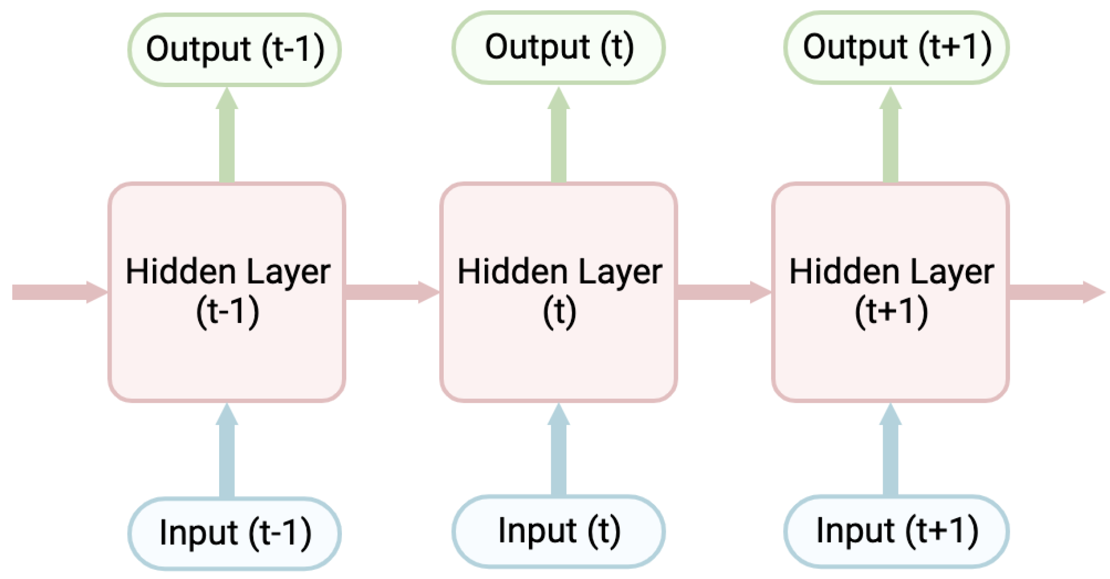
A key difference between Transformers and RNN is their ability to parallelize. Parallelization refers to the technique of dividing the task into smaller sub-tasks that can be executed concurrently. In an RNN, parallelization is prevented because of the limitation of sequential computation. The state sequences at position t are a function of the earlier states at positions t-1 as well as the input for position t, so there is a considerable training dependency (
Figure 1).
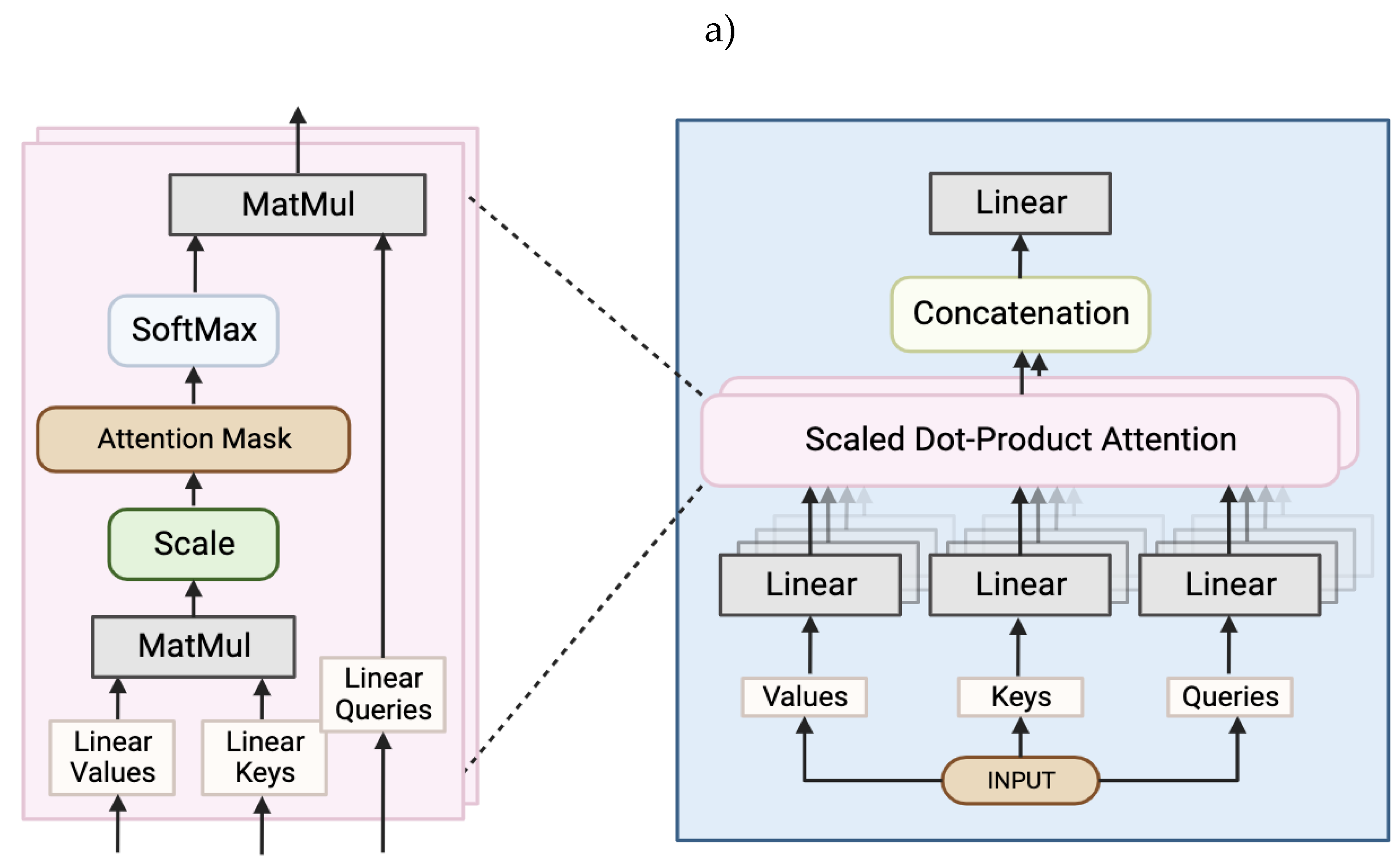
Including attention mechanisms in the neural network (like in a Transformer) can reduce this dependency as the output is computed as a weighted sum of the values mapped to it. The Transformer, on the other hand, relies entirely on an attention mechanism to draw global dependencies between inputs and outputs. One of the sub-layers of the decoder, the multi-head attention, is made up of multiple attention layers that run in parallel (
Figure 2a). These attention layers compute the attention function on linearly projected versions of the queries, keys, and values at the same time which makes the model more efficient, especially when training (Vaswani et al., 2017). The Transformer has been shown to train (and finish training) faster than an RNN while still achieving the same accuracy (Karita et al., 2019).
Previous research in the field of intracortical BCIs by Willett et al. (2021) shows that the current lowest error rate for characters for user-generated sentences is 8.54% in real-time. The participant of this study was a tetraplegic due to a high-level spinal cord injury. He was instructed to attempt to write as if his hand was not paralyzed. The resulting neural activity was recorded by two intracortical microelectrode arrays that had previously been implanted (
Figure 3). These signals were then fed into an RNN which converted the neural population time series into the real-time output by thresholding the probabilities of each character occurring at each time step. Afterward, the output was combined with a vast vocabulary language model, reducing the error rate to 2.25%.
According to Vaswani et al., 2017 and Lee et al., 2023, using a Transformer led to increased accuracy compared to other classifiers which implies the potential to improve upon these error rates if a Transformer is used instead of an RNN. This study aimed to see how a Transformer model, when used in a BCI, compares to the BCI with an RNN and to test the hypothesis that there will be an improvement in the decoded results when using Transformer models (over RNNs) in this context.
METHODS
Dataset
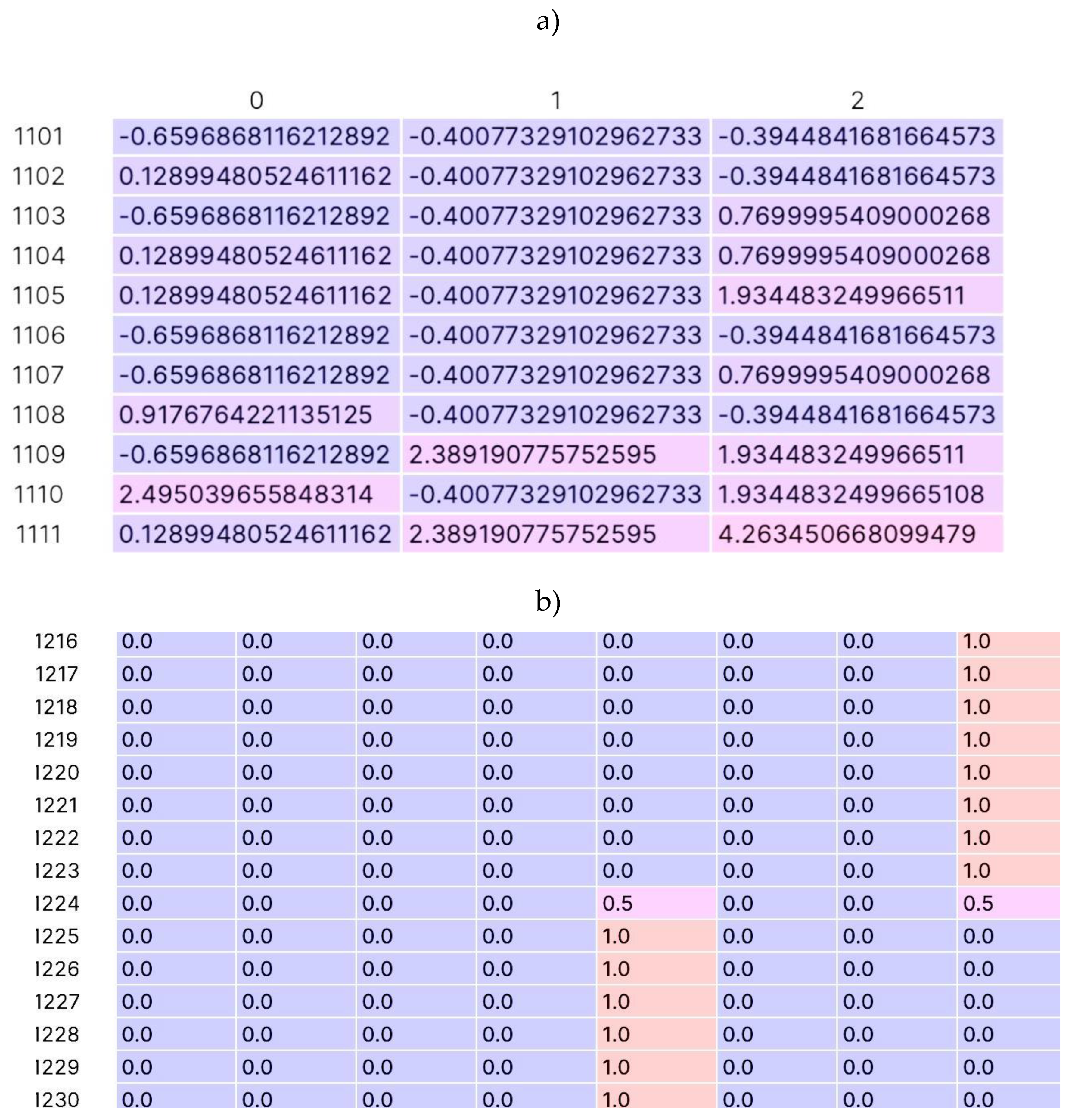
Electrode data was collected from the dataset compiled by Willett et al. (2021). The dataset included 10 sessions over 28 days where data was recorded using two microelectrode arrays (with 96 electrodes each) implanted in the premotor area of the brain of a single participant. This participant had a complex spinal cord injury and was paralyzed from the neck down with hand movements limited to twitching and micromotion. The participant was tasked with writing as if his hand was not paralyzed and was holding a pen on a piece of ruled paper. The dataset included all recorded neural activity (1,000 sentences over 10.7 hours). The data was in the form of binned spike counts, which are integer values corresponding to how many times the voltage on a given electrode crossed a specified threshold during that time bin of 10 milliseconds. There were times when the participant attempted to write full sentences and others when he attempted single letters (
Figure 4).
Model
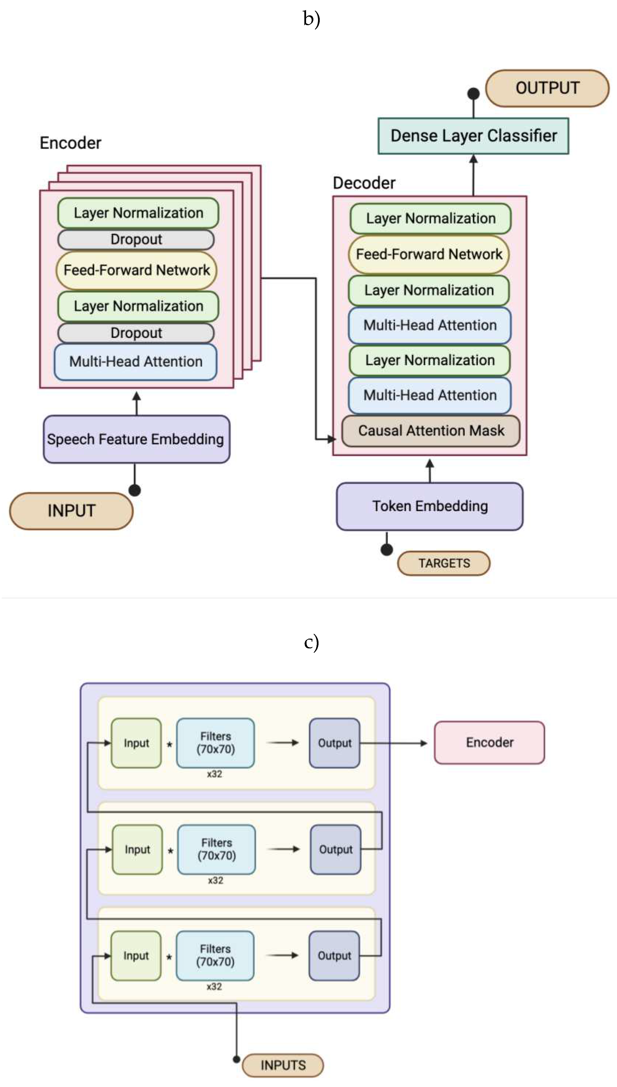
The Transformer had a custom architecture (
Figure 2b), but still had the same key layers that were outlined in the Introduction. Its encoder was made up of a stack of four identical layers. Each had a multi-head self-attention mechanism (
Figure 2a), two dropout sub-layers, a feed-forward network, and two normalization sub-layers.
The decoder was composed of 6 sub-layers: a masked (casual attention mask) multi-head attention over the output of the encoder stack and the targets, three normalization layers, another multi-head self-attention mechanism that was modified to prevent positions from attending to subsequent positions, and a position-wise fully connected feed-forward network. The output embeddings were offset by one position which ensured that the predictions for position i only depended on the known outputs at positions less than i. Before the data was passed to the decoder layers, the data was embedded. This is where the transformer differed from the one proposed in the original Transformer architecture paper (Vaswani et al., 2017). The Transformer in this paper was modeled after Apoorv Nandan’s Transformer (Nandan, 2021). This contained two embedding classes: one for tokens (before the encoder) and one for speech features (before the decoder).
The token embedding class contained the token and positional embedding. The token embedding mapped each individual character to a representative vector of its meaning. The positional embedding was then added to the tokenization which described information about the location of the character in the sentence as each position was assigned a unique representation. This allowed the model to know which letters were further or closer to others and found relationships based on that.
The speech feature embedding class was made up of three 1D convolutional layers (
Figure 2c). The output of each was then fed into the next, and the output of the last was returned as the result. The window size (how many time steps were looked at each time) was more than the average number of time steps per letter to try and fit a letter in each window. The stride (how many time steps the window shifts by) was less than the average to limit shifting by more than a letter each time.
Training
The model was trained to reduce the loss calculated during the testing stage (when the model attempted to translate neural data it hadn’t seen before based on trends noticed during the training phase). The loss function is Categorical Crossentropy, and it is calculated between the one hot encodings of the target sentences and the prediction sentences made by the Transformer. During the training phase, the optimizer (Adam) applied the gradients, computed by GradientTape, of the loss and the trainable variables of the Transformer. Checkpoints were used to save the weights of the model when the testing loss had improved.
RESULTS
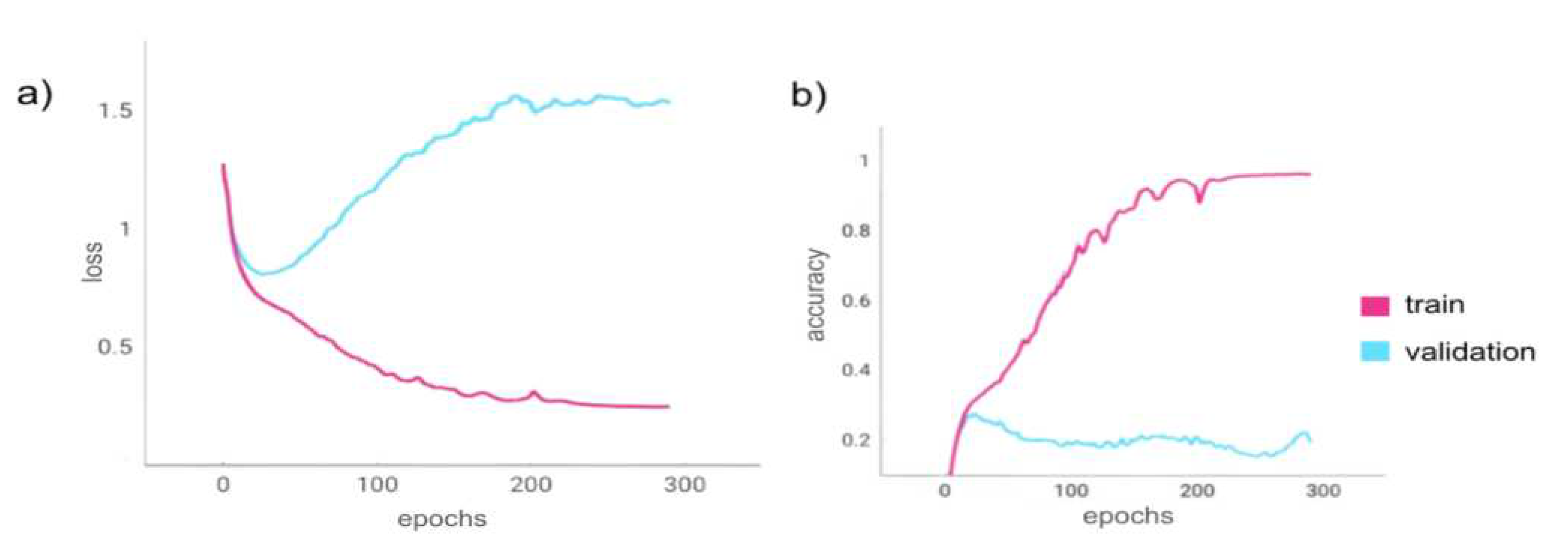
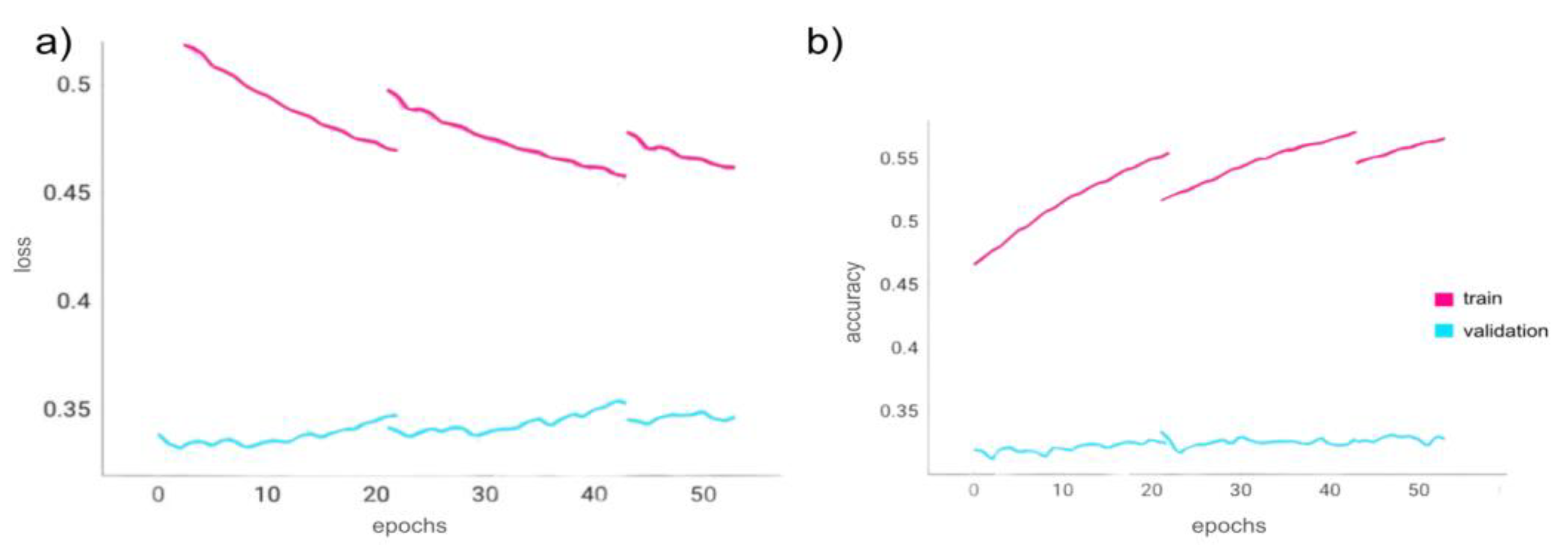
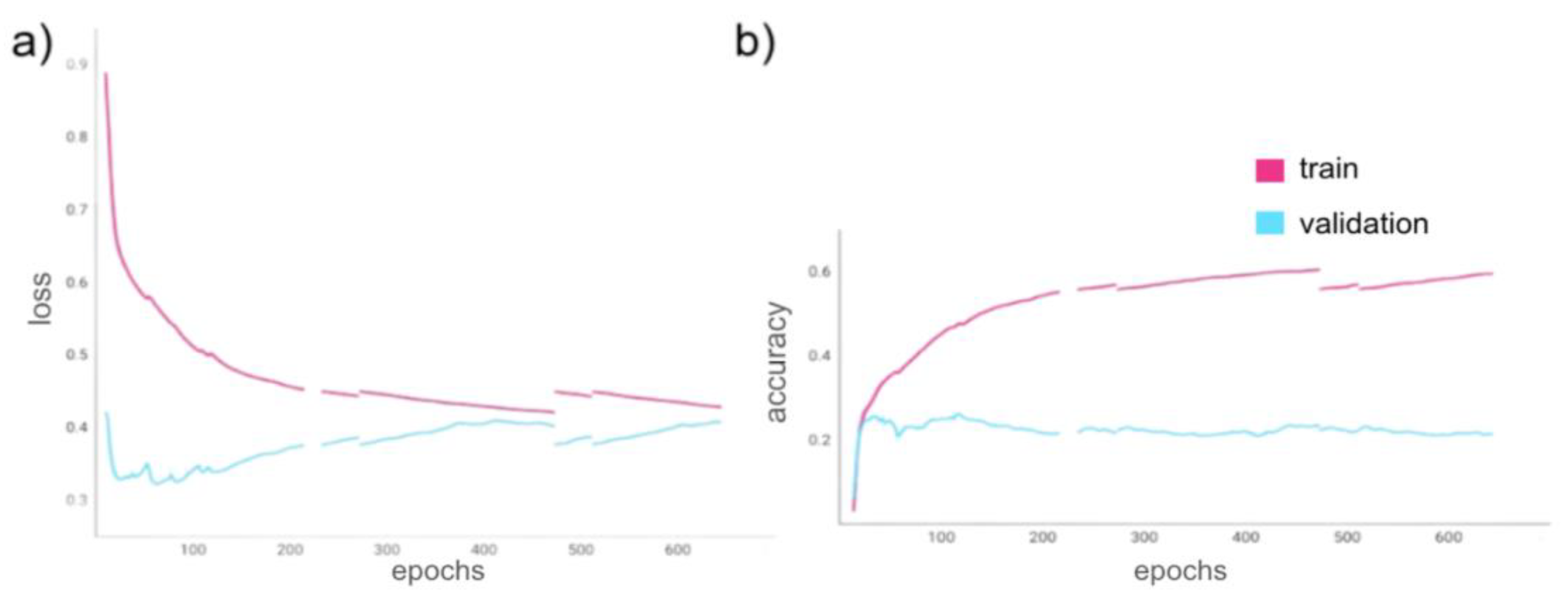
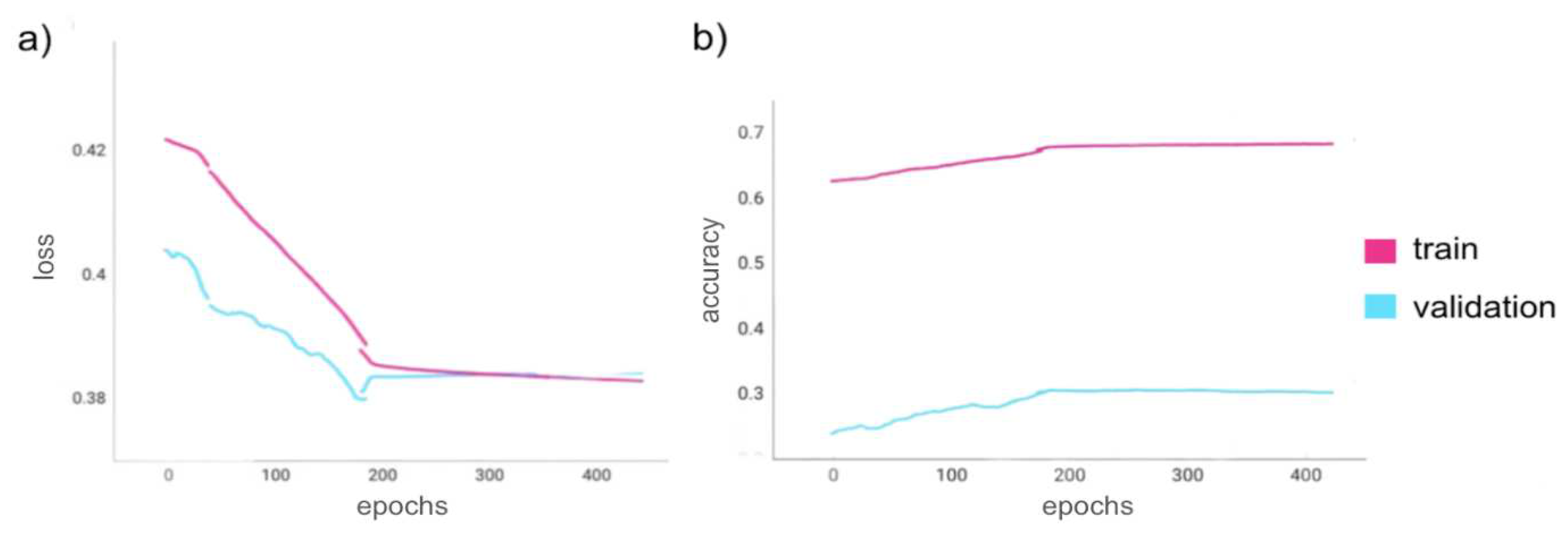
The model was optimized using an Adam optimizer and a custom schedule learning rate. The loss was calculated using a categorical crossentropy function, and accuracy was calculated using categorical accuracy. The graphs (
Figure 5,
Figure 6,
Figure 7 and
Figure 8) show the loss and accuracy (both training and validation) per epoch of the model in each of the four trials. Four trials were performed that tested the model’s ability to find patterns in the inputs and outputs as well as be able to translate the neural signals into sentences when presented with data it had never seen before (validation). The train-validation data split was 90%-10% in all four trials. The first two trials were done with minimal preprocessing of the input signals as the variability in the data was limited in an attempt to test the model’s ability to find the least complex relationships between the inputs and outputs. The last two trials included data augmentation (noise and translations) to see if the model would still be able to find these connections, even with the variability introduced by these processing steps.
Trial 1: Minimizing Loss without Data Augmentation
The model was initially run using a built-in TensorFlow model checkpoint callback that monitored the training loss and saved checkpoints every time it decreased. The data used in this trial was the initial data with only a few basic preprocessing steps (no noise or translations added). The trend portrayed in
Figure 5, proves the model’s ability to overfit as the loss was minimized to 0.25 and the accuracy reached 96.11% while the validation loss ended at 1.54 and the validation accuracy increased to 19.33%. The goal of this trial was not to test the Transformer model’s ability to generalize to the validation data, but rather to show the model’s ability to connect the input data with the output data and find relationships/patterns in the neural signals, which it was successfully able to do.
Figure 5.
Trial 1 epoch loss and epoch acceleration.
Figure 5a,b show the loss and accuracy metrics during Trial 1 as the Transformer model trained for 291 epochs to minimize training loss. The train-validation dataset split was 90%-10% with a training batch size of 3 and a validation batch size of 2. a) Epoch training loss (pink) and epoch validation loss (blue). b) Epoch training accuracy (pink) and epoch validation accuracy (blue). As the program had to be rerun from checkpoints (as there was a software runtime limitation), the graphs are discontinuous at the epochs from which the program restarted.
Trial 2: Minimizing Validation Loss without Data Augmentation
Using the same model checkpoint callback as used in the previous trial regarding the model’s ability to overfit (but instead set to minimize validation loss), the goal of this trial was to see if the same model could generalize the identified patterns to new data, the validation data. The same data was used (with no noise or translations added). As shown in
Figure 6, the trend shows the model’s inability to generalize considerably as the validation loss only decreased to 0.35 and the validation accuracy only increased to 32.51%.
Figure 6.
Trial 2 epoch loss and epoch acceleration.
Figure 6a,b show the loss and accuracy metrics during Trial 2 as the Transformer model trained for 53 epochs to minimize validation loss. The train-validation dataset split was 90%-10% with a training batch size of 3 and a validation batch size of 2. a) Epoch training loss (pink) and epoch validation loss (blue). b) Epoch training accuracy (pink) and epoch validation accuracy (blue). As the program had to be rerun from checkpoints (as there was a software runtime limitation), the graphs are discontinuous at the epochs from which the program restarted.
Trial 3: Minimizing Loss with Data Augmentation
The same model checkpoint was used again (attempting to minimize training loss), but the data in this trial had white noise added to the neural signals (to add variability) which was created using a map to a TensorFlow random normal function. Similarly, the input signals were mapped again to a function that applied a random normal mean drift noise, random walk noise, and cumulative random walk which offset the data by a few time steps. From
Figure 7, the results show a lowest training loss of 0.43 and a highest training accuracy of 62.81%. The validation loss was 0.41 and its accuracy was 24.60% at the end of the last epoch.
Figure 7.
Trial 3 epoch loss and epoch acceleration.
Figure 7a,b show the loss and accuracy metrics during Trial 3 as the Transformer model trained for 632 epochs to minimize training loss using the augmented data. The train-validation dataset split was 90%-10% with a training batch size of 3 and a validation batch size of 2. a) Epoch training loss (pink) and epoch validation loss (blue). b) Epoch training accuracy (pink) and epoch validation accuracy (blue). As the program had to be rerun from checkpoints (as there was a software runtime limitation), the graphs are discontinuous at the epochs from which the program restarted.
Trial 4: Minimizing Validation Loss with Data Augmentation
For the last trial, the (same) model checkpoint callback was used to minimize validation loss. This was trained using the same data with applied transformations as in trial 3 (Minimizing Loss with Noise and Transformations). As can be observed from
Figure 8, this trial showed the least favorable results of a validation loss of 0.39 and a validation accuracy of 31.58%. At the end of the last epoch, the training loss was 0.39 with an accuracy of 69.06%
Figure 8.
Trial 4 epoch loss and epoch acceleration.
Figure 8a,b show the loss and accuracy metrics during Trial 4 as the Transformer model trained for 632 epochs to minimize validation loss using the augmented data. The train-validation dataset split was 90%-10% with a training batch size of 3 and a validation batch size of 2. a) Epoch training loss (pink) and epoch validation loss (blue). b) Epoch training accuracy (pink) and epoch validation accuracy (blue). As the program had to be rerun from checkpoints (as there was a software runtime limitation), the graphs are discontinuous at the epochs from which the program restarted.
DISCUSSION
This study looked at the ability of a Transformer model version of a BCI to see whether the model could translate the neural signals of a paralyzed individual. It was found that this specific implementation of a Transformer BCI did not perform as well as the RNN BCI when comparing the training and validation metrics.
When compared across trials, Trial 2 (minimizing validation data) showed significantly greater loss and decreased accuracy when compared to Trial 1 which showed a successfully overfit model. Similarly, Trial 4 showed less favorable results when compared to Trial 3. Overall, Trials 1 and 2, which were trained using the original data, showed more favorable results as a whole when compared to Trials 3 and 4, which used data that had been transformed slightly. The addition of the random shifts and white noise allowed for the data to differ from the target by a slight amount which would theoretically help the model generalize (as it would allow for slight inconsistencies in the neural signals). However, this addition to the input data (in Trials 3 and 4) did not help the model generalize and even hindered its ability to learn patterns from the training stage (specifically shown in Trial 3).
As suggested by the data, this version of a BCI using a Transformer model was unable to generalize when presented with even the slightest variance from its training data. While the model produced favorable results for the training data in Trial 1, it was unable to generalize the patterns it found to the new data it was presented with, resulting in undesirable metrics for validation data. This was expected as the model was set to minimize the training loss, leading, successfully, to an overfit model that had learned the training examples, not the patterns.
In Trial 2, the validation loss was noticeably greater than the training loss from the overfitting trial, about 1.41 times the amount, while the training accuracy in the overfitting trial was 2.96 times the validation accuracy in this trial. While the model was able to overfit using the training data in the first trial, its unsuccessful attempt at minimizing the validation loss in this trial shows it was unable to generalize this knowledge to the validation data. Unlike in Trial 1, the model was set to minimize validation loss, so it should have learned patterns instead of specific examples. However, these unfavorable results indicate the model’s inability to find the patterns between the neural signals and the characters in the intended sentence text.
In comparison to Trial 1 (overfitting with unprocessed data), Trial 3 has a significantly greater training loss (0.43 vs. 0.25) and a significantly lower training accuracy (62.81% vs. 96.11%). While the model used to be able to learn the correlation between the inputs and outputs in the training dataset (as shown in Trial 1), the model was unable to do the same thing this time when even the slight variability was included of noise and transformations to the dataset. This is further evidence of the model’s inability to generalize, even slightly.
Trial 4 clearly performed the worst when compared to all previous trials (specifically Trial 2: minimizing validation loss without noise or transformations). The model was not able to recognize patterns (as required when minimizing validation loss) and apply them to new data when the transformations had been applied. As the variability of the data increased from Trial 2 to this trial through the additions of minor transformations, the model performed poorly (high validation loss and low validation accuracy).
The original RNN BCI calculated the loss of the character probabilities and the start signal (when a new character began) separately. The character probability loss was calculated using softmax cross-entropy and was then summed with the start signal loss (a sigmoid computation) to produce the total loss. The reported character loss was 0.09. The accuracy was 94.1% when a k-nearest-neighbor classifier was applied to the character probabilities outputted by the model (Willett et al., 2021). In the Transformer model, the loss was calculated by comparing the predicted characters to the correct characters; no starting character loss was implemented. The character validation loss in the trial that most closely reproduced the RNN BCI (Trial 4), was 0.39 with a validation accuracy of 31.58%. The lower error and higher accuracy of the RNN BCI suggest that it produces more favorable results than the Transformer BCI.
As mentioned in Vaswani et al., 2017 and Lee et al., 2023, a benefit of the Transformer model over an RNN is its ability to translate more accurately. When compared to the results of the RNN BCI, however, this Transformer model performed less favorably in all trials. A reason for this seemingly contradictory result could be their usage of synthetic data in training. Synthetic data was made up of a compilation of random corresponding snippets of the collected neural signals and the intended handwritten text. The device used for training this Transformer model had limited GPU storage, resulting in an inability to add synthetic data to the dataset due to its load on the GPU and time constraints limiting the possibility of finding and implementing another solution. Using a GPU is a critical part of AI model training and the size of its storage has an impact on the model’s performance (Baji, 2017; Jeon et al, 2021; Li et al., 2022) A greater amount of data has the potential to improve the model’s ability to generalize as it sees potential variation that is allowed for each character reinforced through multiple examples (Cai & Hu, 2020). The significantly reduced amount of data used to train this model could have led to this Transformer model being unable to generalize despite the data augmentation (Wang et al., 2016). Another potential reason is stopping the training too early as it may have reached a more favorable outcome had it been allowed to continue training for longer.
While this study shows this Transformer model’s inability to generalize even slightly, there are several limitations that should be noted. For one, the model was trained on a single device with a single GPU, severely restricting the amount of data that the model was able to train on in a given time window. Also, because of a time constraint due to approaching deadlines, the training of the model for each trial was terminated after 2-4 days, leading to a potential underrepresentation of the model’s ability to generalize.
The current scope of the project did not explore the difference in training speed between the RNN BCI and this Transformer BCI, something that would be an interesting avenue to investigate. As indicated by Karita et al., 2019 and Vaswani et al., 2017, a Transformer is generally able to train much more efficiently, due to its increased parallelization, than an RNN, something that would be a noteworthy improvement over its predecessor. A way to do this could be recording the training time for multiple batches of data per model, finding the median (or mean), and then dividing by the number of examples in a batch. This value could then be compared for the RNN and the Transformer models. Another potential extension is including the synthetic data in the Transformer model and seeing how that affects the results. We would expect to see an improvement in the metrics, specifically in the validation ones. To do this, a GPU with a greater storage capacity would be needed (or work could be split up on multiple GPUs), or the code could be set to load in individual examples/batches one at a time. The RNN BCI also implemented an offline autocorrect process by sending the outputs from the RNN through a large-vocabulary language model. Comparing the results of the autocorrection on the Transformer output versus the RNN output could result in interesting discoveries about the necessity of an offline autocorrection.
References
- Baji, T. (2017, July). GPU: the biggest key processor for AI and parallel processing. In Photomask Japan 2017: XXIV Symposium on Photomask and Next-Generation Lithography Mask Technology (Vol. 10454, pp. 24-29). SPIE.
- Cai, W., & Hu, D. (2020). QRS complex detection using novel deep learning neural networks. IEEE Access, 8, 97082-97089. [CrossRef]
- Coin, A., Mulder, M., & Dubljević, V. (2020). Ethical aspects of BCI technology: what is the state of the art?. Philosophies, 5(4), 31. [CrossRef]
- Jeon, W., Ko, G., Lee, J., Lee, H., Ha, D., & Ro, W. W. (2021). Deep learning with GPUs. In Advances in Computers (Vol. 122, pp. 167-215). Elsevier. [CrossRef]
- Karita, S., Chen, N., Hayashi, T., Hori, T., Inaguma, H., Jiang, Z., ... & Zhang, W. (2019, December). A comparative study on transformer vs rnn in speech applications. In 2019 IEEE Automatic Speech Recognition and Understanding Workshop (ASRU) (pp. 449-456). IEEE.
- Kumar, M. K., Parameshachari, B. D., Prabu, S., & liberata Ullo, S. (2020, September). Comparative analysis to identify efficient technique for interfacing BCI system. In IOP Conference Series: Materials Science and Engineering (Vol. 925, No. 1, p. 012062). IOP Publishing. [CrossRef]
- Nandan, A. (2021, January 13). Keras Documentation: Automatic speech recognition with Transformer. Keras. keras.io/examples/audio/transformer_asr/.
- Lee, P. L., Chen, S. H., Chang, T. C., Lee, W. K., Hsu, H. T., & Chang, H. H. (2023). Continual learning of a transformer-based deep learning classifier using an initial model from action observation EEG data to online motor imagery classification. Bioengineering, 10(2), 186.
- Li, Y., Phanishayee, A., Murray, D., Tarnawski, J., & Kim, N. S. (2022). Harmony: Overcoming the hurdles of GPU memory capacity to train massive DNN models on commodity servers. arXiv preprint arXiv:2202.01306. [CrossRef]
- Vaswani, A., Shazeer, N., Parmar, N., Uszkoreit, J., Jones, L., Gomez, A. N., ... & Polosukhin, I. (2017). Attention is all you need. Advances in neural information processing systems, 30.
- Wang, H., Lei, Z., Zhang, X., Zhou, B., & Peng, J. (2016). Machine learning basics. Deep learning, 98-164.
- Willett, F. R., Avansino, D. T., Hochberg, L. R., Henderson, J. M., & Shenoy, K. V. (2021). High-performance brain-to-text communication via handwriting. Nature, 593(7858), 249-254. [CrossRef]
- Wolpaw, J. R., Birbaumer, N., Heetderks, W. J., McFarland, D. J., Peckham, P. H., Schalk, G., ... & Vaughan, T. M. (2000). Brain-computer interface technology: a review of the first international meeting. IEEE transactions on rehabilitation engineering, 8(2), 164-173. [CrossRef]
|
Disclaimer/Publisher’s Note: The statements, opinions and data contained in all publications are solely those of the individual author(s) and contributor(s) and not of MDPI and/or the editor(s). MDPI and/or the editor(s) disclaim responsibility for any injury to people or property resulting from any ideas, methods, instructions or products referred to in the content. |
© 2023 by the authors. Licensee MDPI, Basel, Switzerland. This article is an open access article distributed under the terms and conditions of the Creative Commons Attribution (CC BY) license (http://creativecommons.org/licenses/by/4.0/).
