1. Introduction
In their old age, people tend to have one form of disease or another related to their condition. One such condition is the Parkinson’s disease. It is a neurological condition that affects the human brain [
1]. It causes tremors in the body and hands, as well as stiffness in the body [
2]. As of now, this disease has no proper cure or treatment. It can only be treated when the condition is diagnosed early, or at its inception. This will not only lower the cost of treatment but may also save lives. Most available methods can detect Parkinson’s disease in its advanced stages, indicating a loss of most of the dopamine in the basal ganglia. The basal ganglia is responsible for coordinating bodily movement with a small amount of dopamine. In the United Kingdom alone, more than 145,000 people have been identified as suffering from the disease, whereas in India, nearly one million people are affected by this condition according to a study conducted by Aljalal et al. [
3].
After Alzheimer’s disease (AD), Parkinson’s disease (PD) is the second most common human neurodegenerative condition with an annual incidence of 10–18 per hundred thousand persons. The most common risk factor reported in their study was age, which has serious public health implications. At some stages, PD may cause tremors, stiffness, and difficulties in walking, balancing, and coordinating movements in affected individual [
4].
Some of the symptoms of Parkinson’s disease normally appear gradually and worsen over time. People examined and diagnosed with Parkinson’s disease may have difficulties walking and speaking as the disease continues to develop [
2]. In their study Kurmi et al., [
5] stated that the victims of Parkinson’s disease may also have mental and behavioral changes, as well as sleeping difficulties, depression, memory problems, exhaustion, and so on. Parkinson’s disease affects both men and women. However, men are affected to a greater extent by the condition than are their female counterparts. Age is clearly a high-risk factor for Parkinson’s disease. That is, the higher the age, the greater the tendency to contract the disease. Although the majority of people with Parkinson’s disease develop the disease around the age of fifty-five, it was further revealed that approximately five to ten percent of persons with Parkinson’s disease develop it before the age of 50 years. Parkinson’s disease is generally but not always hereditary, and some forms are related to specific genetic mutations [
4].
There are many indications or signs of the disease, but the four main signs of Parkinson’s disease are found to be stiffness of the limbs and trunk tremors (trembling) of the hands, arms, legs, jaw, or head movement, indicating low balance and coordination, which can lead to falls. Others include depression and other mood changes, trouble eating, chewing, and speaking Bladder issues or constipation, skin problems, and sleep disruptions are all possible symptoms of Parkinson’s disease [
2]. Nevertheless, the aforementioned studies had a detection rate of approximately 96% but failed to improvise the data. Therefore, we improved the quality of the PD detection model to design improved gradient boosting algorithms.
The difficulty in obtaining accurate data from patients with PD may be due to their old age and variations in patient characteristics. The technique was designed to automatically monitor the medication state of patients using supervised machine learning techniques such as random forest, support vector machine, k-nearest neighbor, and naïve Bayes. Parkinson’s disease detection accuracy is not yet 100 %, as a result, this study aimed to improve it using an extreme gradient boosting algorithm [
1].
This study will significantly benefit both patients and medical personnel. This will help unveil an up-to-date detection model for Parkinson’s disease. This study has the potential to improve the work of medical facilities in the detection and treatment of diseases.
The salient contributions of this study are as follows:
Design of a machine learning framework for the detection of Parkinson’s disease using supervised machine learning algorithms.
Exploration and highlighting of the effects of Parkinson’s disease (PD) using supervised machine learning models.
Performance evaluation of models for PD detection using performance evaluation metrics.
2. Related Works
There are several kinds of studies found in the literature that were carried out to detect Parkinson’s disease using various techniques, including machine learning and deep learning; however, boosting methods were the least explored in the detection of Parkinson’s disease. Fujita et al., [
6] conducted a study that detected Parkinson’s disease (PD) constructing using a detection model that combined a recurrent neural network (RNN) and convolutional neural network (CNN), focusing on the fact that patients with Parkinson’s disease (PD) have motor speech disorders. Mei and Desrosiers reviewed literature on Parkinson’s disease [
7].
The study conducted compared the performance of the RNN to that of the long short-term memory (LSTM) and gated recurrent unit (GRU) with conventional gates [
8]. In this study, graphene-based biosensors were used to detect dopamine for effective Parkinson’s disease diagnostics. Biosensors are being converted into smartphone-connected disease management systems. However, they emphasized that clinical utility should take precedence over analytical and technical performances.
In a similar study, Hoq et al., [
4] used machine learning classifiers to detect PD. The probe results showed that the proposed sparse autoencoder—support vector machine (SAE-SVM) model outperformed not only the previous model of the principal component analysis-support vector machine (PCA-SVM) and other standard models, such as multilayer perceptron (MLP), extreme gradient boosting (XGBoost), K-Nearest Neighbor (KNN), and random forest (RF), but also two recent studies using the same dataset.
To detect the presence of Parkinson’s disease, using vocal tasks for remote detection and monitoring has provided highly accurate results in numerous trials of (PD). However, most of these studies published results based on a small number of voice recordings, which are often taken under acoustically controlled conditions and thus cannot be scaled up without the use of specialized equipment [
8].
Finding accurate biomarkers that allow the development of medical decision support tools is now a major research effort in healthcare biometrics. These instruments aid in the detection and monitoring of disorders, such as Parkinson’s disease [
1].
CNN has been used to diagnose Parkinson’s disease (PD) from drawing movements. Feature extraction and classification are two main aspects of a CNN. The best results obtained in their study were 96.5 % accuracy, F1-score of 97.7 %, and area under the curve of 99.2 % [
9].
The difficulty in obtaining accurate data from patients with PD may be due to their age and variations in patient characteristics. The process was designed to automatically monitor the medication state of patients using supervised machine learning techniques such as random forest, support vector machine, k-nearest neighbor, and naïve Bayes. Random forest outperformed the other models in performance [
10].
Patients with Parkinson’s disease are more likely to experience fluctuations in their motor symptoms. This unavoidable trait may affect the quality of life of patients. However, utilizing self-reported data from PD makes it challenging to gather precise information on fluctuation features. Based on the outcome of the research by the authors, Aich et al., [
11] concluded that the possibility of employing inertial sensors incorporated into commercial smartphones was proven in their work, which also presented a simple technique for accurate postural instability grading. This tool can be used to detect the early indicators of Parkinson’s disease, monitor the disease, and prevent falls.
In their study, Aljalal et al., [
3] proposed an automated Parkinson’s disease detection method using deep learning. EEG recordings from 16 healthy controls and 15 PD patients were used in this study. EEG recordings were transformed into spectrograms using the Gabor transform, which was then utilized to train the proposed two-dimensional convolutional neural network (2D-CNN) model. The proposed model achieved high classification accuracy. However, some diseases would have already caused significant damage before their discovery.
Most similar or related works found in the literature either used deep learning or machine learning methodology and image and voice recognition to detect or diagnose Parkinson’s disease in the early stages or later [
12,
13]. By contrast, this study analyzes and evaluates state-of-the-art models using a machine learning classifier for the accurate and timely detection of PD. In addition, we have tried to explain what Parkston’s disease is, its symptoms, causes, and cure in simple terms.
2.1. Disease Detection
Detection of diseases in human beings or any other living creature is of paramount importance and dates from the first existence of man on Mother Earth. Therefore, detecting Parkinson’s disease and other related ailments in persons of all ages, especially elderly people, cannot be overstressed.
2.2. Boosting Machine Learning Classifiers
Boosting refers to the process of making a weak learner become a better and efficient. Therefore, the boosting algorithm is based on the idea of turning least-performing models or classifiers into a better and more efficient models [
14]. The first boosting algorithm was Adaptive Boosting or, for short, AdaBoost, followed by Gradient Boosting, and presently it is eXtreme Gradient Boosting algorithm. Gradient boosting (GBoost) is an ensemble-learning technique developed to improve the efficiency of binary classifiers. Adaptive Boosting employs an iterative strategy to improve poor classifiers by learning from their mistakes. Weak AdaBoost learners comprise decision trees with a single split. AdaBoost works by placing more weight on not-easy-to-classify cases and less weight on those that are already well classified. Fresh weak learners are introduced in stages, allowing them to concentrate on more difficult forms [
10].
The adaptive boosting algorithm was generalized as a gradient boosting algorithm. Gradient boosting is a commanding collaborative machine-learning method. It is a popular method for structured predictive and detective molding problems, for example, descriptive/classification and continuous/regression on tabular data, and is frequently used as the main classifier or one of the major classifiers used in endearing results and clarifications in many, if not all, machine learning competitions [
1].
Various applications of gradient boosting algorithms are available, including but not limited to standard implementations in Python, such as SciPy, and many other efficient third-party libraries. Most systems use different platforms and names to implement this algorithm [
10].
2.3. Dataset
A dataset is a collection of raw statistics and data gathered during a research project [
15]. The dataset is central to study work such as this because it tells us the history and behavior of certain quantities, measurements, and diseases. The PD dataset was generated and obtained from a popular repository for machine learning research [
16]. The dataset used is described in Subsection 2.4.1. and 2.4.2.
2.3.1. Parkinson’s Data Set
The dataset used for this study was collected from popular machine learning repositories, the UCI Machine Learning repository, and Kaggle [
https://archive.ics.uci.edu/ml/datasets] [
17] and [
https://www.kaggle.com/datasets] [
18]. Max Little of the University of Oxford generated the dataset in partnership with the National Center for Voice and Speech in Denver, Colorado, which records speech signals. The data were downloaded in a comma-separated value (CSV) format, as shown in
Table 1.
2.3.2. Dataset Information
Table 1 lists the features and descriptions of the PD dataset. This dataset contains a variety of biological voice measurements from 31 individuals, 23 of who have PD. Each column in the table refers to a specific voice measure, and each row corresponds to one of the 195 voice recordings made by these persons. The primary goal of the data is to distinguish healthy persons from those with Parkinson’s disease using the “status” column, which is set to 0 for healthy people and 1 for those with PD [
19].
3. Methodology
3.1. The Proposed Model Framework
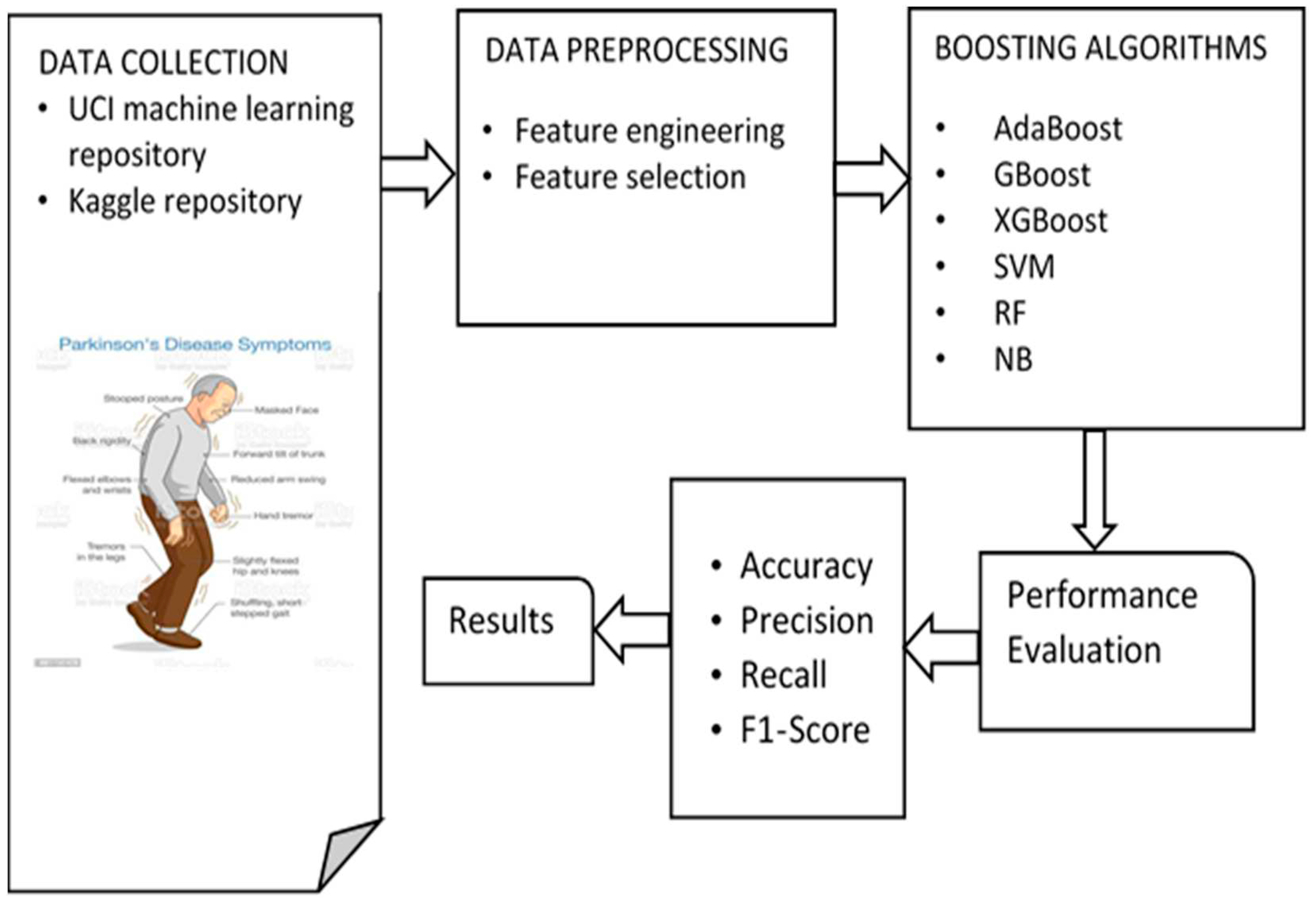
Figure 1 illustrates the methodology of the proposed performance evaluation framework. This study used different datasets to determine the best-performing model and for the ease of evaluation and reporting of the results. The datasets were downloaded from the UCI machine learning and Kaggle repositories [
17,
18]. Data manipulation techniques such as data preparation and feature selection were performed. Subsequently, the dataset was divided into two parts: training and testing. The models built are subjected to training data to learn from its pattern and evaluated on the testing data to determine the accuracy, precision, recall, and f1-score. Therefore, this study deployed a relatively new method for improved disease detection using a supervised machine learning algorithm.
3.2. Working Principle of the Model
The principle of the proposed performance evaluation framework for supervised machine learning algorithms is shown in
Figure 1. The framework provides all the steps required to achieve the desired improvement or improved prediction performance for PD. The PD datasets were downloaded from the two repositories and loaded. The datasets underwent preprocessing. After working on the data, the dataset was divided into two parts: training and testing. The implemented models were subjected to training data for learning and were evaluated on the dataset reserved for testing. The results obtained were evaluated using performance evaluation metrics for classification to further determine and investigate hidden patterns.
3.3. Experimental Setup Procedure
First, all programs, tools, and techniques needed to perform this experiment were downloaded and installed to obtain good results. The Python libraries used for various operations and functions were also installed. These included NumPy [
20] which is used for numerical Python, pandas [
21] used for data loading and analysis and is also acquired and installed to prepare the environment. Jupyter Notebook [
22] was used to present the codes and data well. The Scikit-learn [
23] Python machine learning library was used for designing, building, and developing machine learning classifiers, such as extreme gradient boosts.
3.3.1. Data Gathering
This is the first step for most, if not all, machine-learning detection projects. Data is the first thing we need to acquire to start developing and running machine learning projects. The quality of the data s central to obtaining good and accurate detection at the end of the experiment. As a result, the data used in this research paper as stated above was obtained from a reputable machine learning repository which is known as the UCI machine learning repository [
17]. The data obtained are comma-separate values (. csv) format.
3.3.2. Data Preparation
The necessary support programs, files, and datasets for research were imported. Data preparation is paramount and is used to prepare the data such that it is appropriate for the machine-learning project. The collected data were loaded into a Google Labs notebook. It is common knowledge that most collected or downloaded data must be prepared or preprocessed to fit the proposed model and obtain an accurate and dependable result. Therefore, the obtained data underwent data preprocessing, feature extraction, and feature engineering, as briefly explained in the following subsections.
3.3.3. Data Preprocessing
This is a crucial step in machine learning detection and classification. This process is used to enhance the quality of a dataset to promote the extraction of meaningful and accurate insights. It is a tool and technique used in machine learning projects for cleaning and organizing data to make them suitable for building, training, and testing machine learning models ). This was applied in this study to transform the raw data into an understandable and readable format [
13].
3.3.4. Feature Extraction
This feature extraction step is a process of dimensionality reduction in which an initial set of data is reduced by identifying only the most relevant key features from the dataset that affect the detection by the machine learning model.4 In this study, feature extraction is used to select the relevant features necessary for PD detection.
3.3.5. Feature Engineering
This feature is also primarily used to improve or enhance the accuracy of model detection performance. It is a machine learning technique that leverages data to create new variables that are not in the training dataset [
11]. It generally produces new features for both supervised and unsupervised machine learning projects. It is used to simplify and increase the speed of dataset transformation and manipulation, in addition to improving the precision, recall, f1-score, and accuracy of the model performance.
3.4. Train-Test Split
The bulk of the machine learning algorithm research is used to train the model because the accuracy of the machine learning model mostly depends on the model training on the dataset. After the model was developed and trained, testing was necessary to measure the accuracy of its detection performance. At this stage, the dataset was divided into two sets containing 65 % and 35 % of data; the first set for training and the second for testing, and this was performed to evaluate the model performance on a dataset that was not known to the model.
4. Performance Evaluation
It is important to evaluate the results of the model to determine what is needed, whether it is accurate, and can be deployed to serve the purpose for which it was developed. The ultimate goal of any machine learning model is to learn from examples in such a way that the model can apply what it has learned to new situations that it has not previously encountered. At the most basic level, one should train on a portion of the complete dataset, leaving the rest for evaluation, to determine the model’s capacity to generalize; in other words, determine how well the model performs on data that it has not directly learned from during training [
24].
4.1. Parameter Tuning
Before building the XGBoost model, we must examine the various parameters and their values. Therefore, parameter adjustment is required to increase and completely exploit the advantages of the XGBoost model over the competing methods. Various parameter combinations were tested until a better performance was finally discovered.
4.1.2. Choice of Evaluation Metrics
The detection problem is a classification problem. Therefore, to evaluate the performance of supervised machine learning, we used a confusion matrix that uses accuracy, precision, recall, and f1 scores. These evaluation metrics were used to evaluate the disease detection models [
25,
26,
27,
28].
4.1.3. Confusion Matrix
A confusion matrix is a summary of the predicted outcomes of the classification problem [
5]. The number of rights and unsuccessful predictions are totaled and broken down by class using count values. The confusion matrix depicts various ways in which the classification model becomes perplexed when making predictions. It provides information, not only about the faults made by the classifier, but also the types of errors that are being made. This breakdown addresses the drawback of relying solely on categorization accuracy. The numbers of rights and unsuccessful predictions are totaled and broken down by class using the count values. The confusion matrix depicts various methods by which the detection or classification model becomes perplexed when making predictions. It informs you not only about the errors made by your classifier, but also the types of errors that are being made [
2].
| Event |
No-event |
| Event |
True Positive (TP) |
False Positive (FP) |
| No-event False Negative (TN) |
True Negative (TN) |
|
4.1.4. True Positive (TP)
These are successfully predicted positive values, indicating that the value of the real class is positive, as well as the value of the anticipated class. For example, if the actual class value indicates that the patient survived, the anticipated class also suggests that the patient survived [
1].
4.1.5. False Positive (FP)
This occurs when the expected class is yes and the actual class is no. For example, if the actual class indicates that this patient did not survive, the forecasting class indicates that this patient will [
28,
29,
30,
31,
32,
33].
4.1.6. False Negative (TN)
This occurs when the actual class is positive, and the anticipated class is negative. For example, if a patient’s actual class value indicates that he or she survived, the predicted class value implies that the person would die. Once these four characteristics are understood, the accuracy, precision, recall, and F1 scores can be calculated [
12].
4.1.7. True Negative (TN)
These are accurately predicted negative values, indicating that the value of the real class is zero, and that of the projected class is zero. For example, if the real class states, the patient does not survive, and the forecasting class is the same. False positives and false negatives occur when the actual class differs from the projected class [
5].
4.1.9. Accuracy
The simplest intuitive performance metric is the accuracy, which is the ratio of correctly predicted observations to all observations. We believe that, if our model is accurate, it will be optimal. Accuracy is a useful statistic, but only when the datasets are symmetric and the values of false positives and false negatives are almost equal. Consequently, other parameters must be considered when evaluating the model’s performance [
4].
where the meanings of the parameters in Equations (1)–(4) are as follows.
= True Positive
= True Negative
= False Positive
= False Negative
4.1.10. Precision
The ratio of accurately predicted positive observations to the total expected positive observations is known as precision. The question that this measure answers is how many patients were identified as having survived. A low false-positive rate is related to high precision [
5].
4.1.11. Recall
Yes, recall is defined as the ratio of accurately predicted positive observations to all observations in the class. Many surviving patients were labeled according to this question. Recall is also referred to as sensitivity [
1].
4.1.12. F1-Score
Precision and Recall are weighted and averaged, respectively. This study considered the use of the F1-Score metric and incorporated both false positives and false negatives. Although not as intuitive as the accuracy, F1 is frequently more useful than the accuracy, particularly if the class distribution is unequal. Accuracy works well when false positives and false negatives have equivalent costs. It is best to consider both precision and recall if the costs of false positives and false negatives are considerably different [
4].
5. Results and Discussion
In this section, we explain the stages involved in acquiring data for the experimental procedure and present the results. The data cleaning methods used in this study are also described. The evaluation, analysis, and discussion of the results obtained are also included in this section.
The evaluation parameters used to assess the machine learning algorithms were accuracy, average recall, average precision, and average f1 score. To comprehend the total accuracy of performance, a specific task was used. The recall is determined for each class in the present scope of the task and indicates the number of data samples that the model properly identifies for a given class.
The average percentage of accurate predictions (True Positive and True Negative) for each class was computed using the average recall. In addition, the accuracy of the forecasts was computed, which established confidence in a specific forecast. Moreover, average precision was computed for the purpose of evaluation, allowing us to determine the average of all precision ratings for each class. Finally, the f1-score was computed, which provided a weighted average of the precision and recall of each class. Penalty was imposed on the score for each sample in a class that was incorrectly predicted. The generalizability of the generated model to incoming unseen data is another issue that must be addressed because it is employed in the production environment.
Table 2 provides an overview of the experimental results. All classifiers were run using the same platform and conditions. Five models, namely extreme gradient boosting, random forest, support vector machine, k-nearest neighbor, and naïve Bayes, were applied. The results obtained are listed in
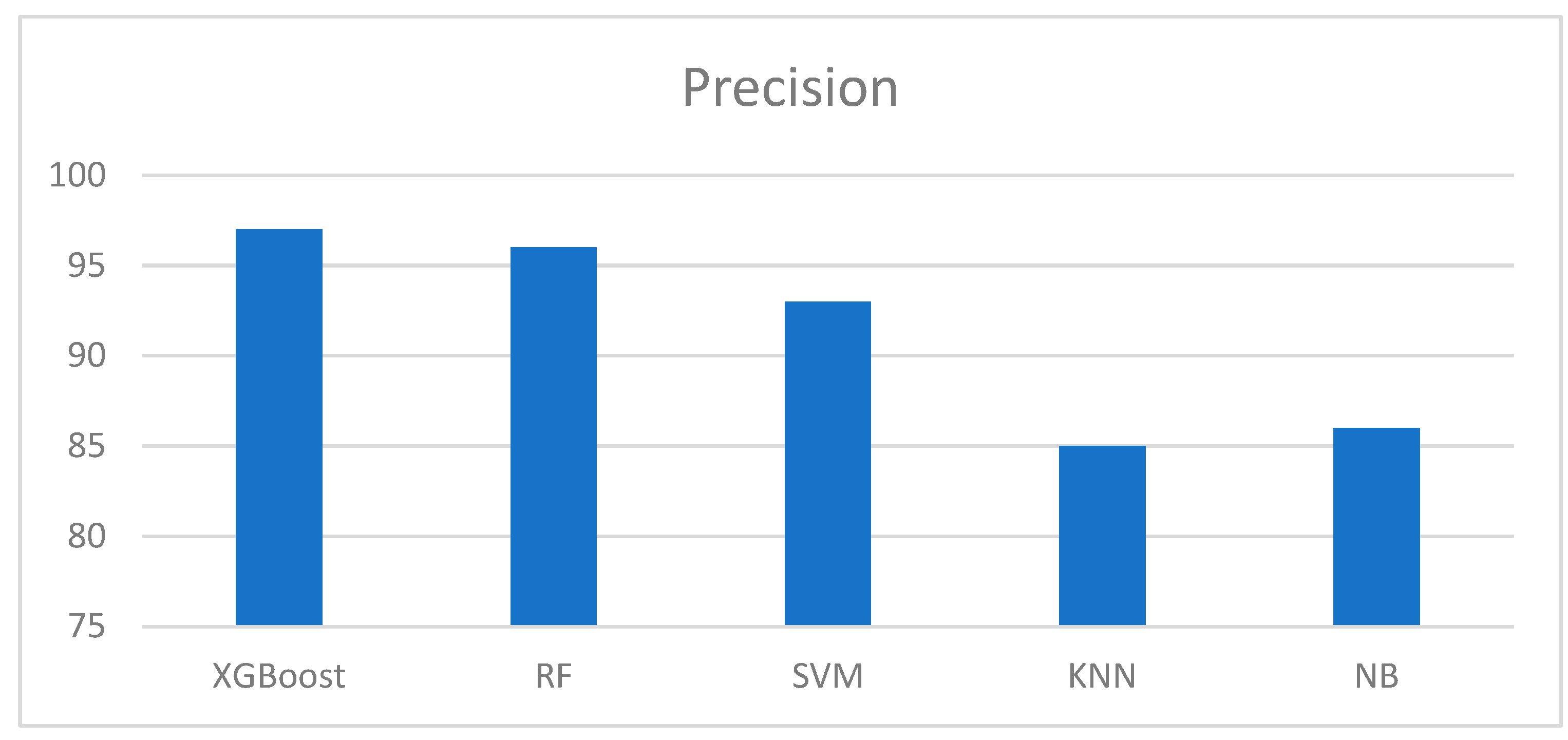
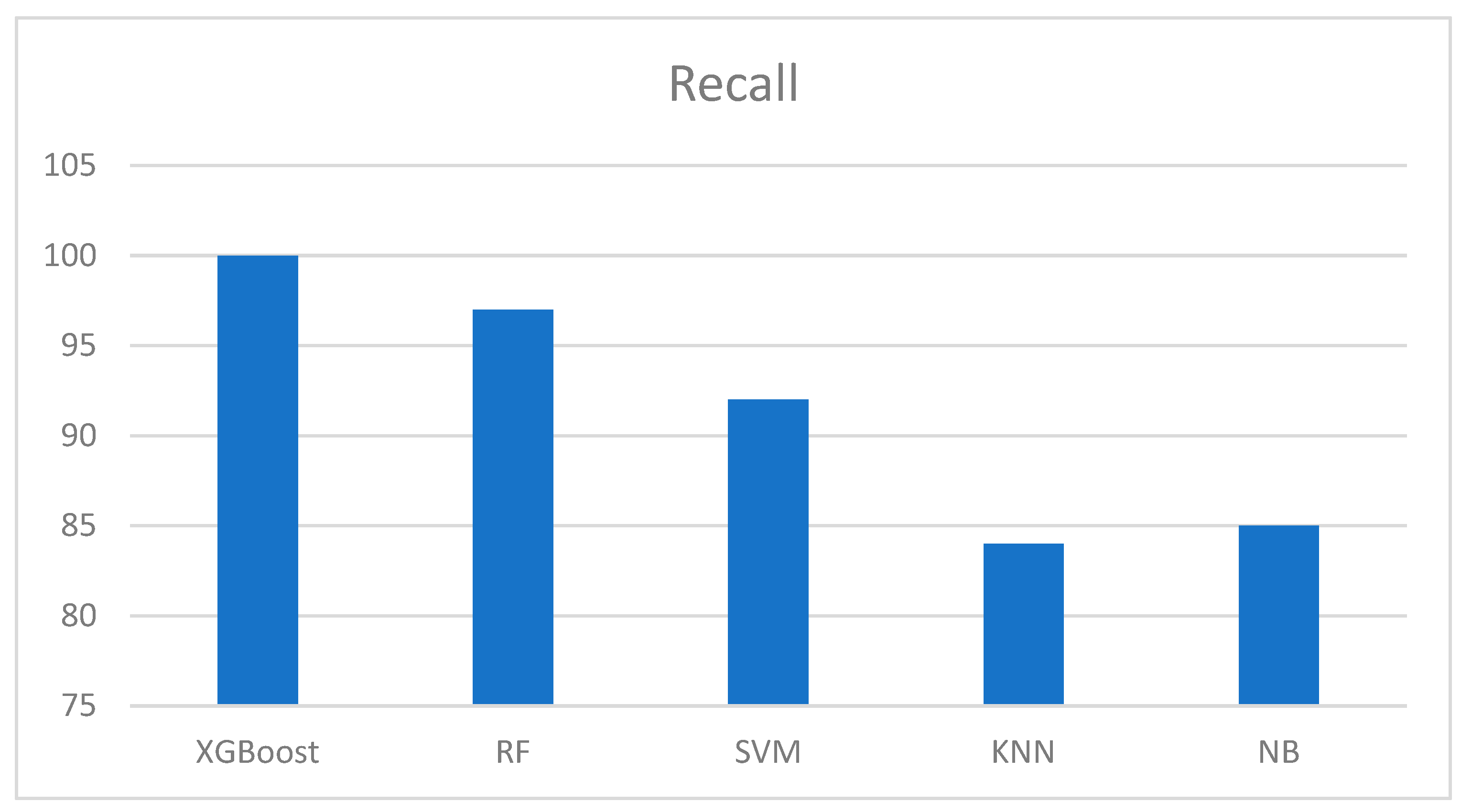
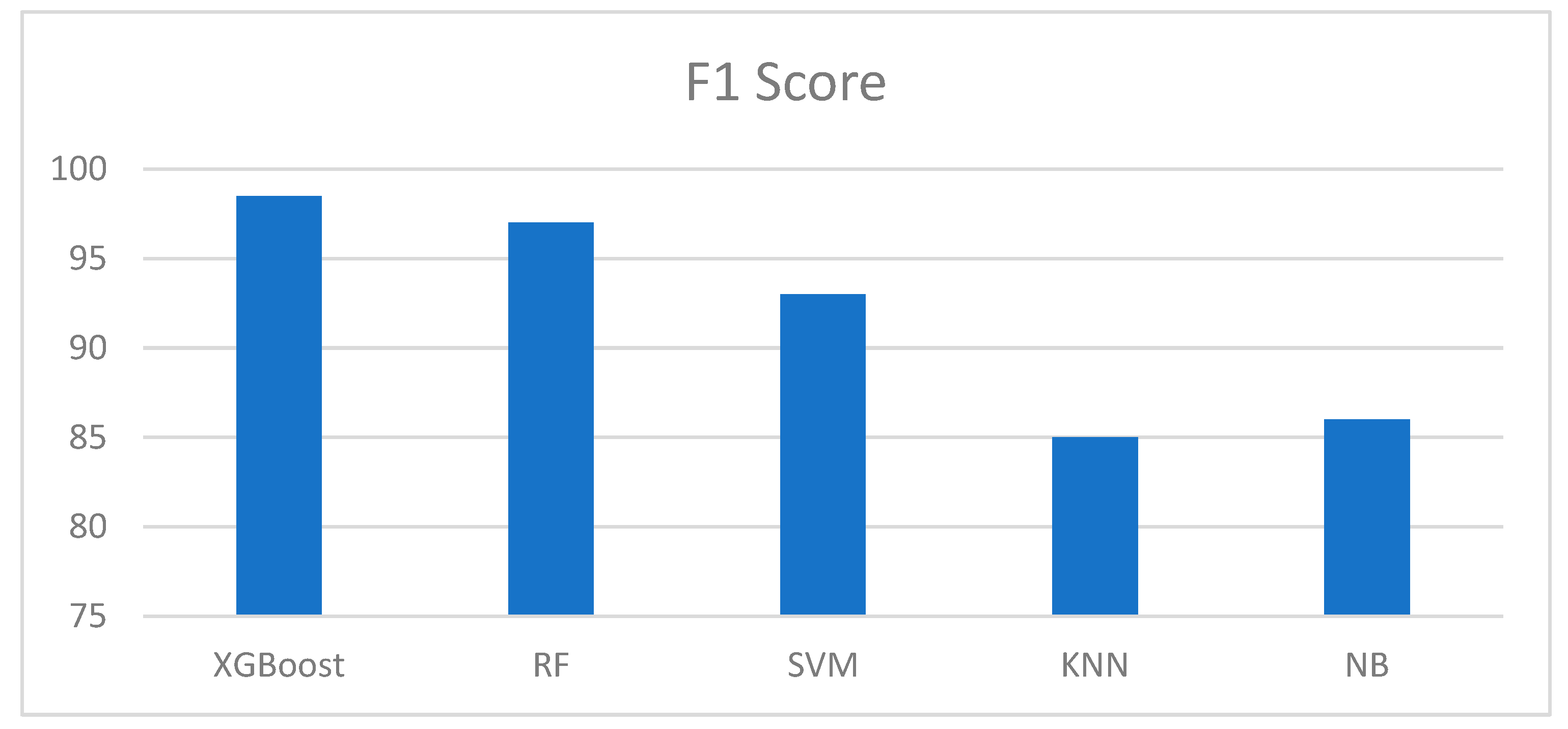
Table 2, with the extreme gradient boosting method exhibiting the highest accuracy and precision. It also has a recall of hundred percent and 98.5% f1-score. In essence, the boosting classifier outperformed all the other models used in previous studies.
5.1. Data Description
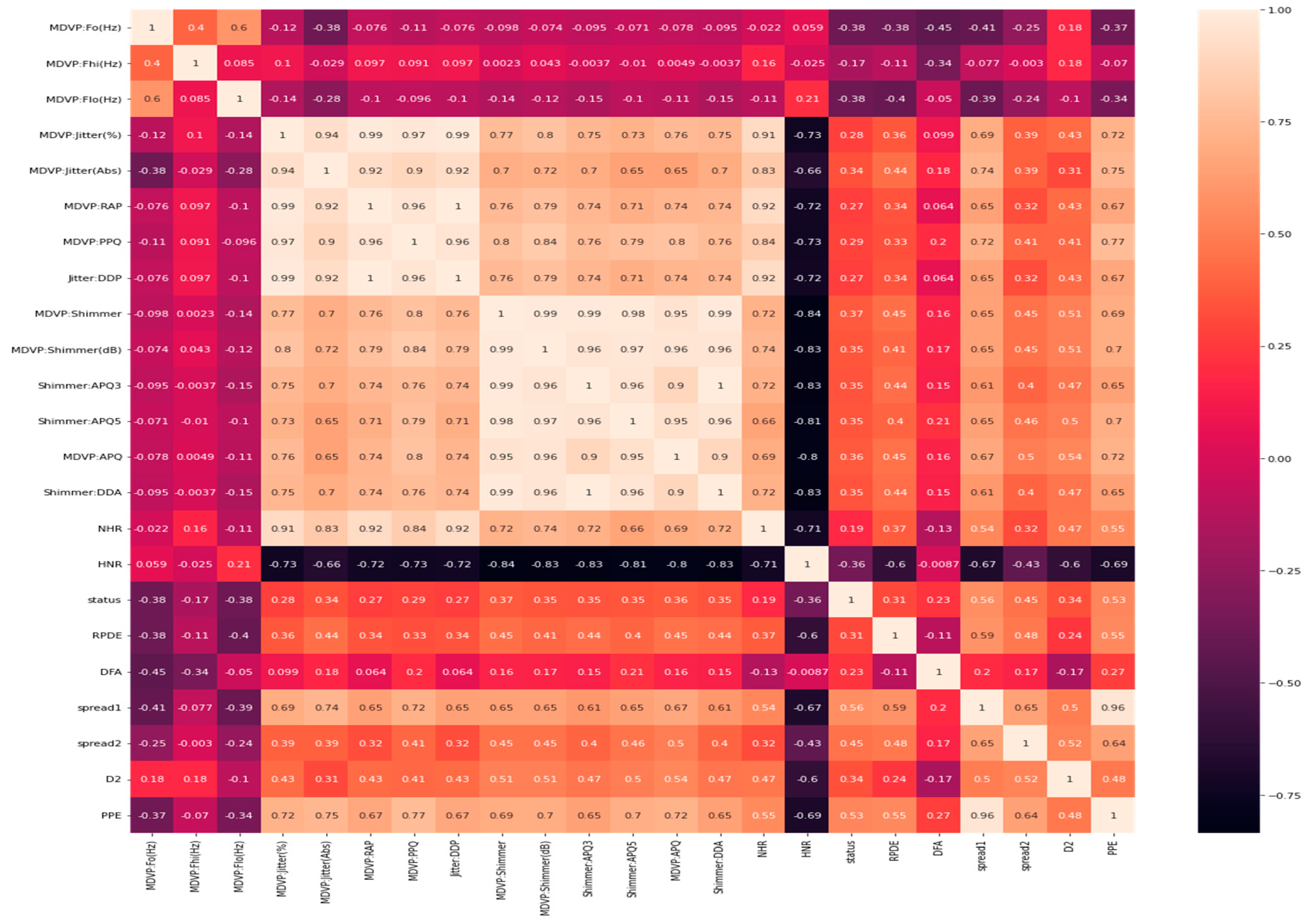
Google Colab supports various frameworks for data description and analysis, and several pieces of information can be derived from these data. The data shape, information, and correlation were explored to clearly understand the dependent is an independent variable, and their relationships.
Figure 2 shows the relationships between the various columns in the datasets. It is obtained using a Python library called Seaborn. The black to white color ratio indicates a very low correlation to a very high correlation, that is, from minus one to plus one. The cells in black show no relationship, whereas the cells in white show an excellent correlation.
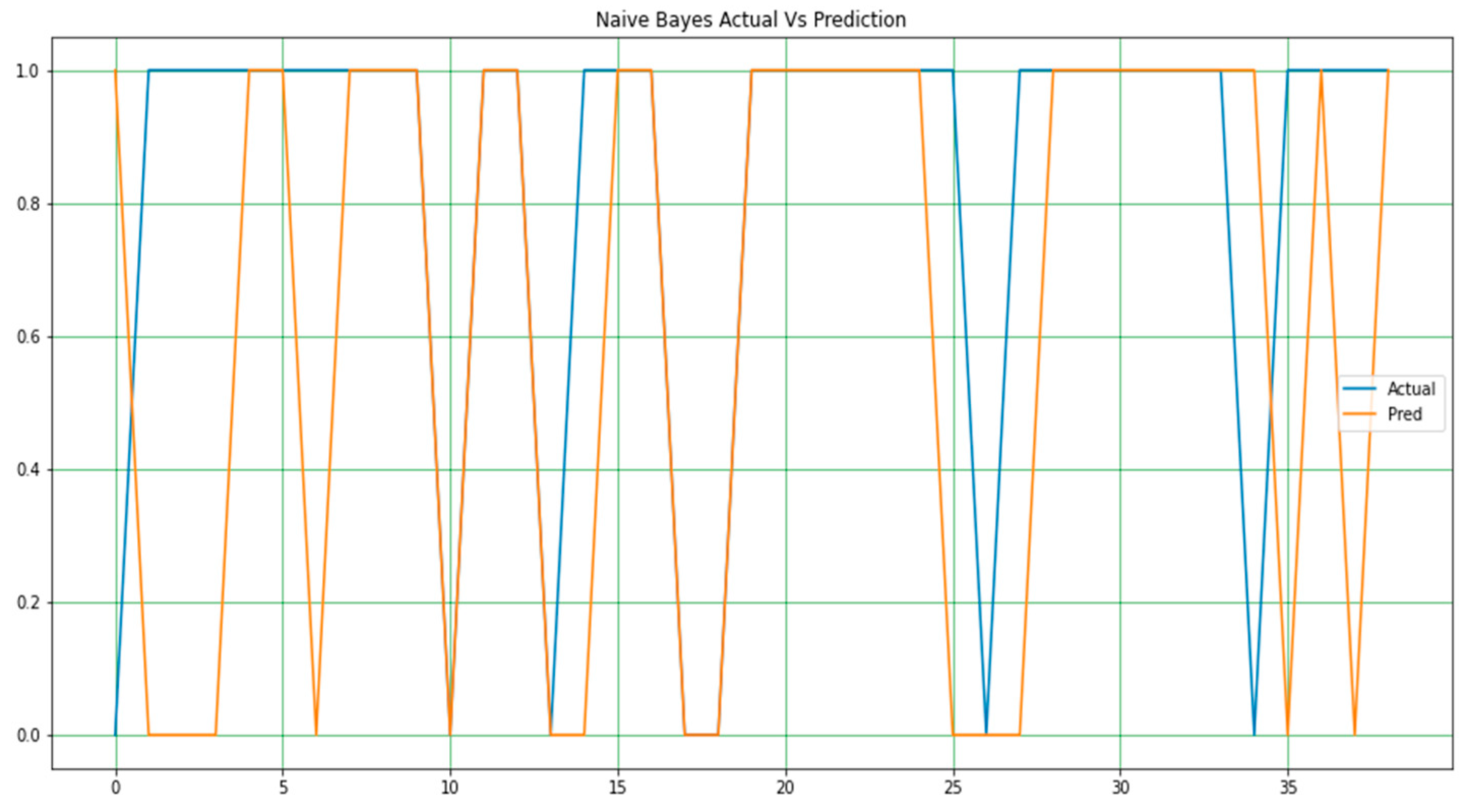
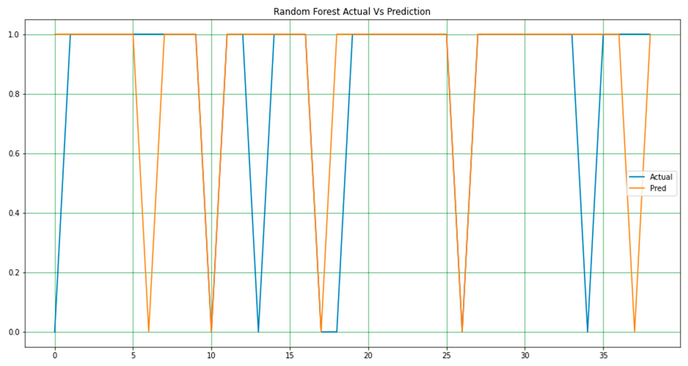
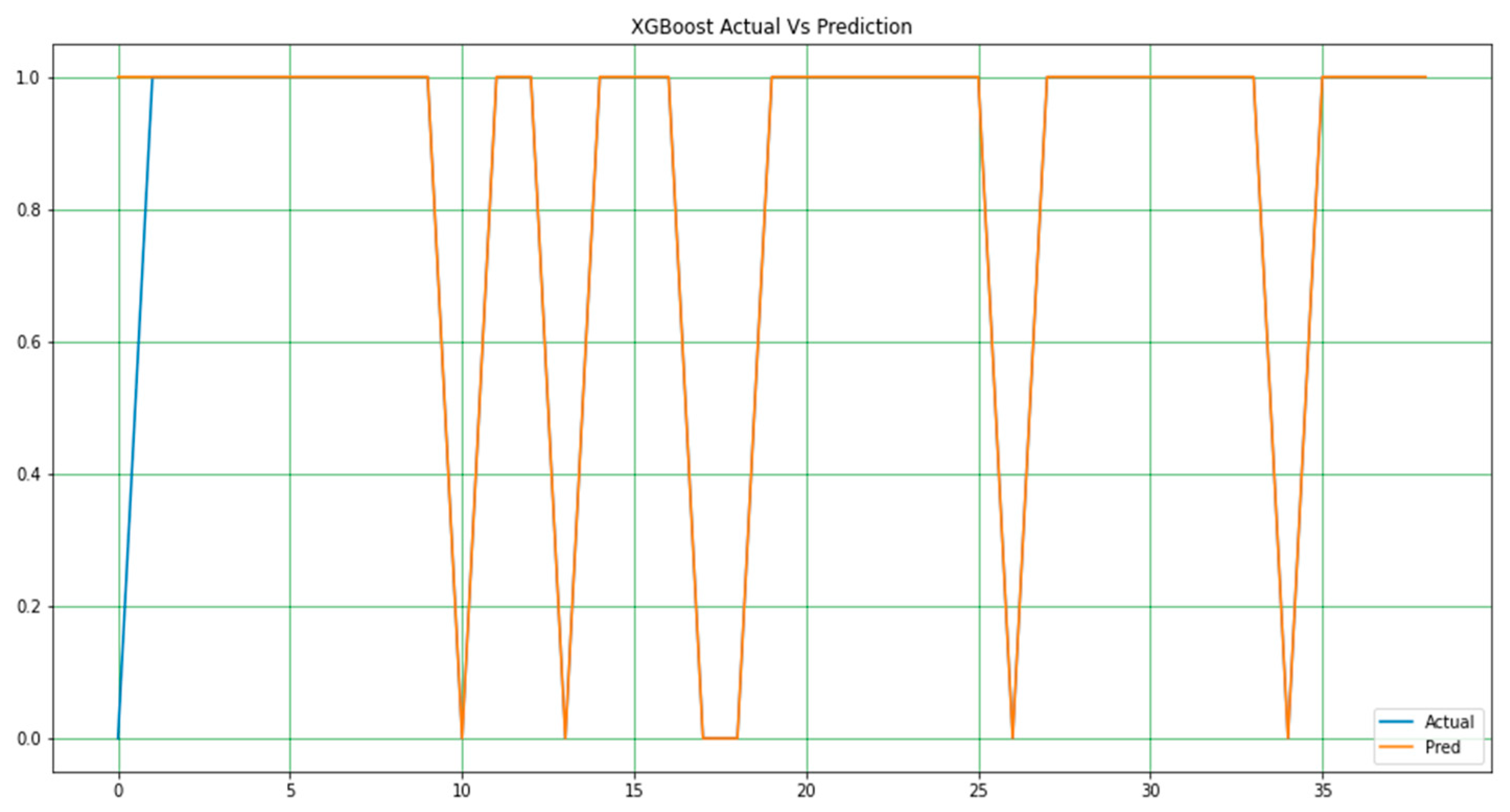
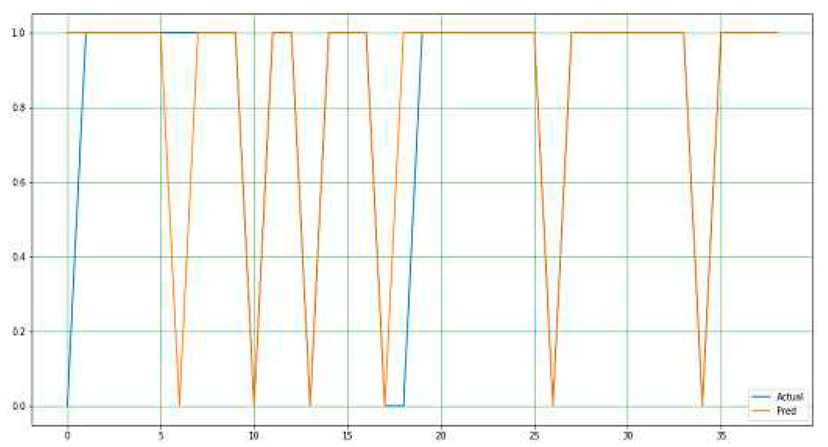
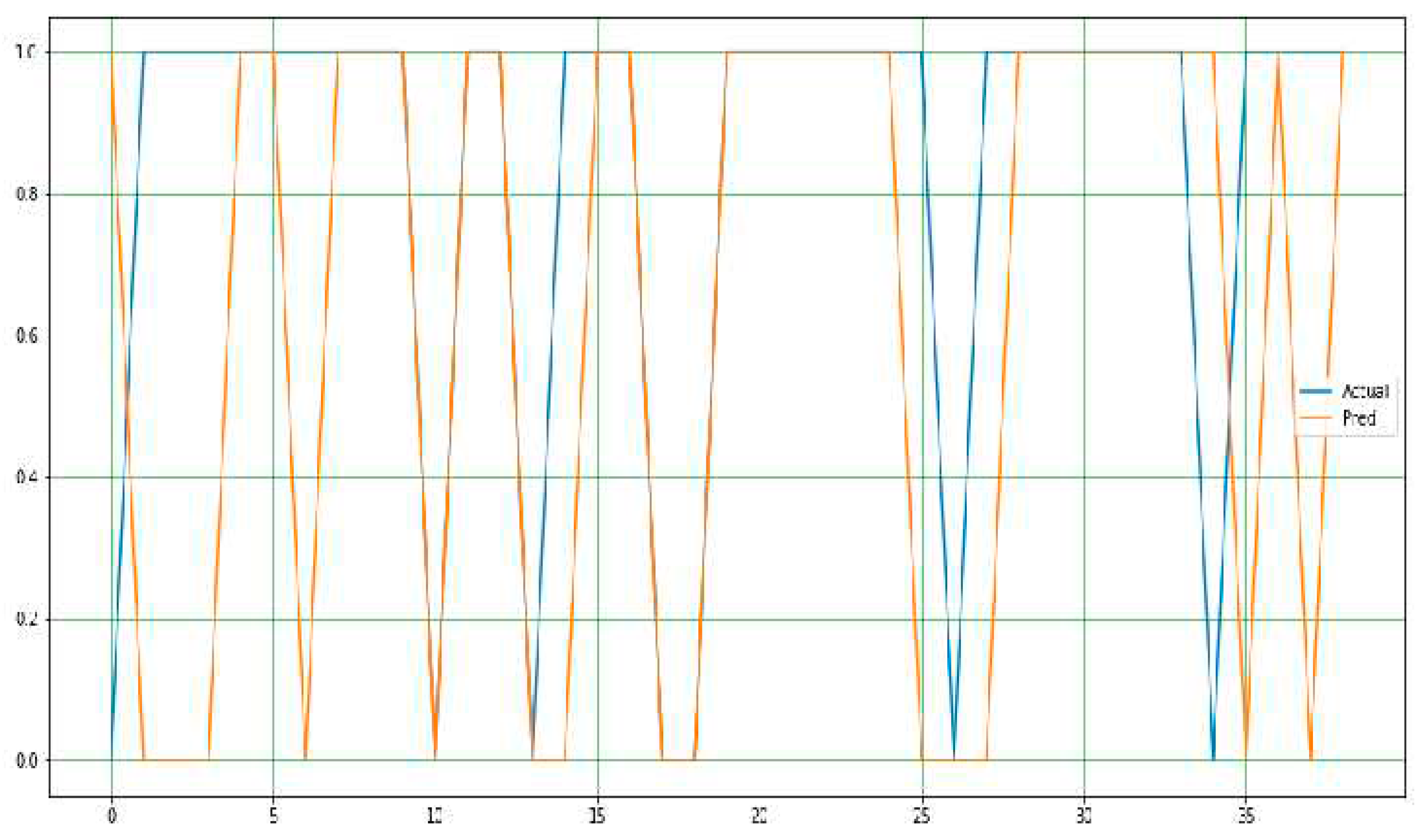
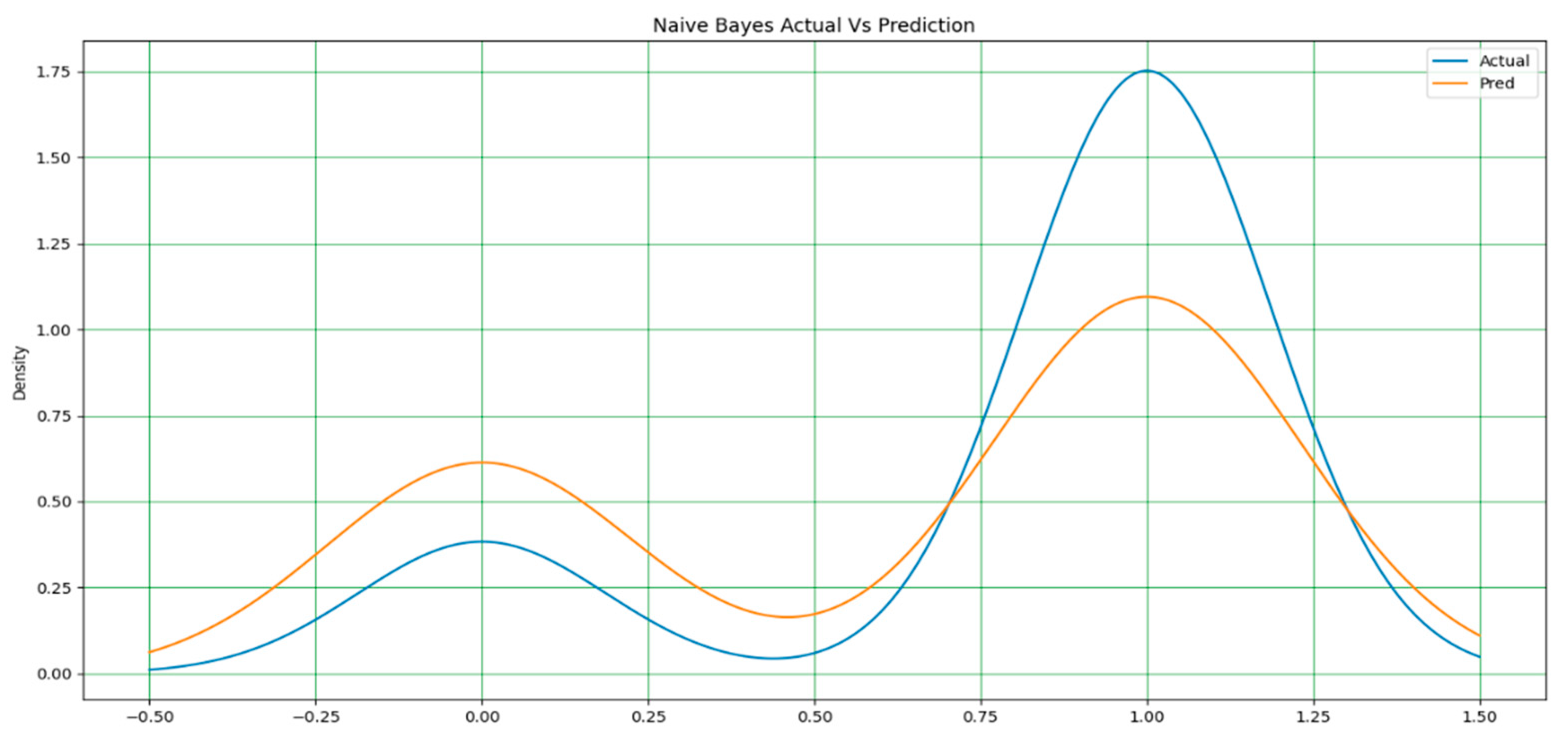
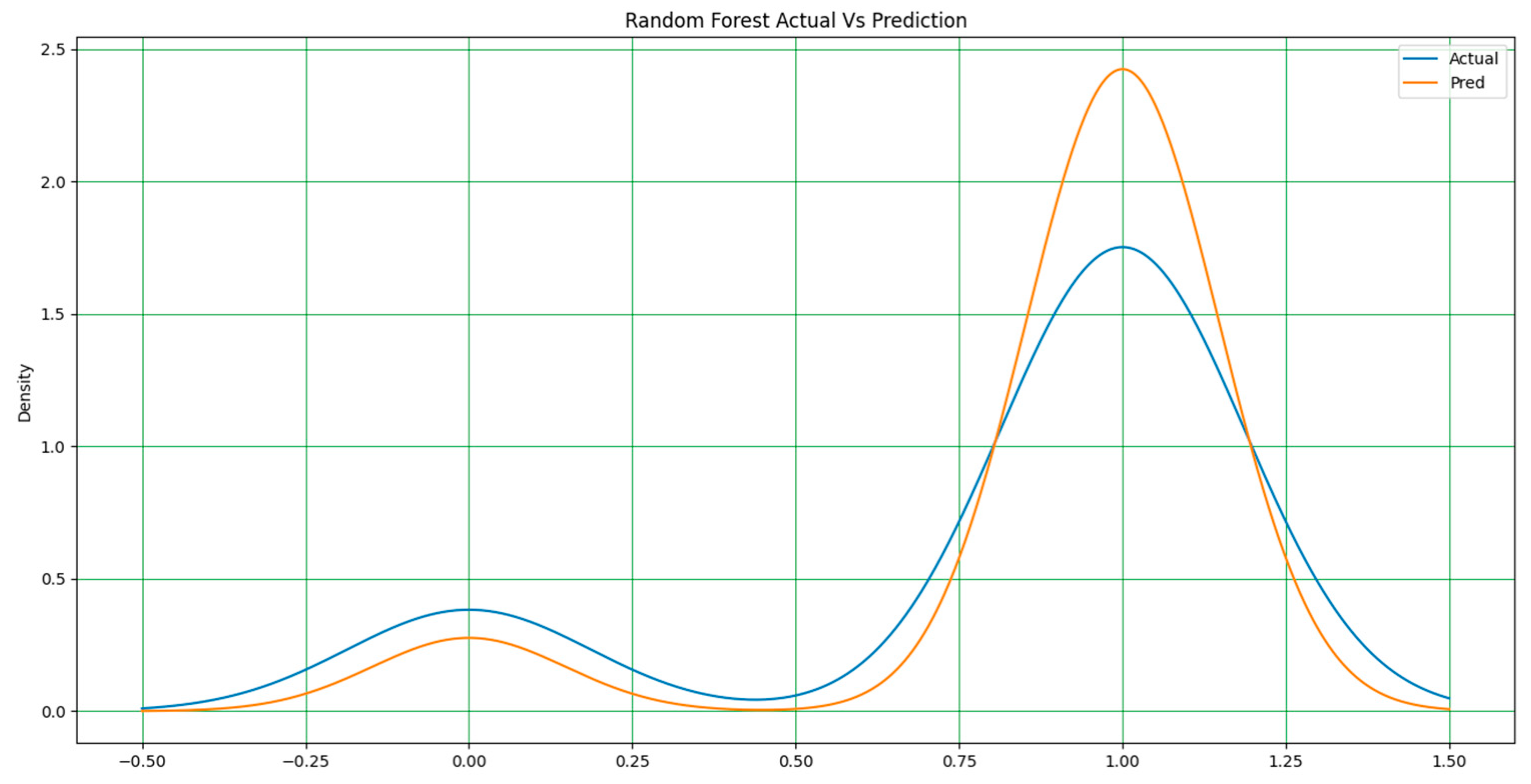
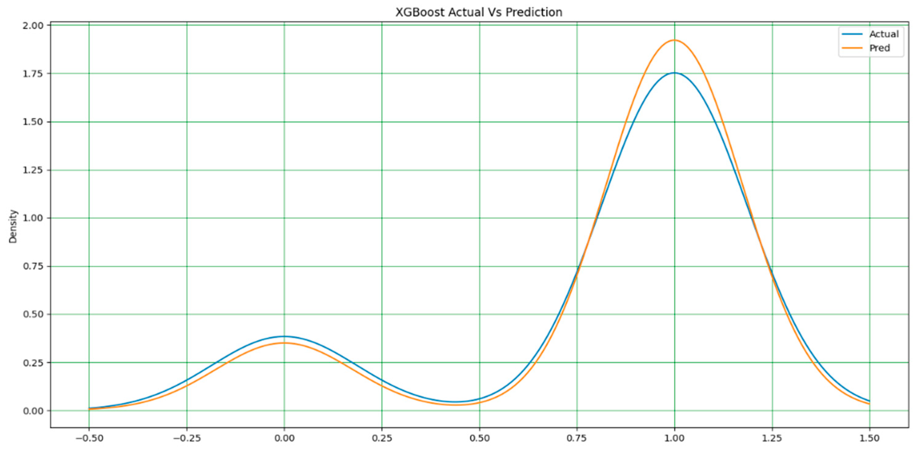
It should be noted that in all the figures, x-axis represents the predicted value and the y-axis represents the period. In
Figure 3,
Figure 4 and
Figure 5, a line-type plot was used to plot the actual versus predicted values. The blue lines indicate the actual values of the dataset and the orange lines represent the prediction results.
Figure 3 illustrates the naïve Bayes prediction results compared to the actual data. For the random forest algorithm in
Figure 4, the difference between the actual and predicted values is not as clear as that in naïve Bayes, but it is one way to obtain the actual prediction.
As stated earlier, the extreme gradient boost in
Figure 5 outperformed all models in terms of performance accuracy and other evaluation metrics. It has a nearly perfect prediction, and the difference between the actual and predicted values is minimal; hence, it requires a simple adjustment to achieve a perfect output. The two lines in this plot represent the accuracy achieved by the model.
Figure 6 and
Figure 7 display the actual and predicted performances of the support vector machine and k-NN, respectively.
Figure 8,
Figure 9,
Figure 10 and
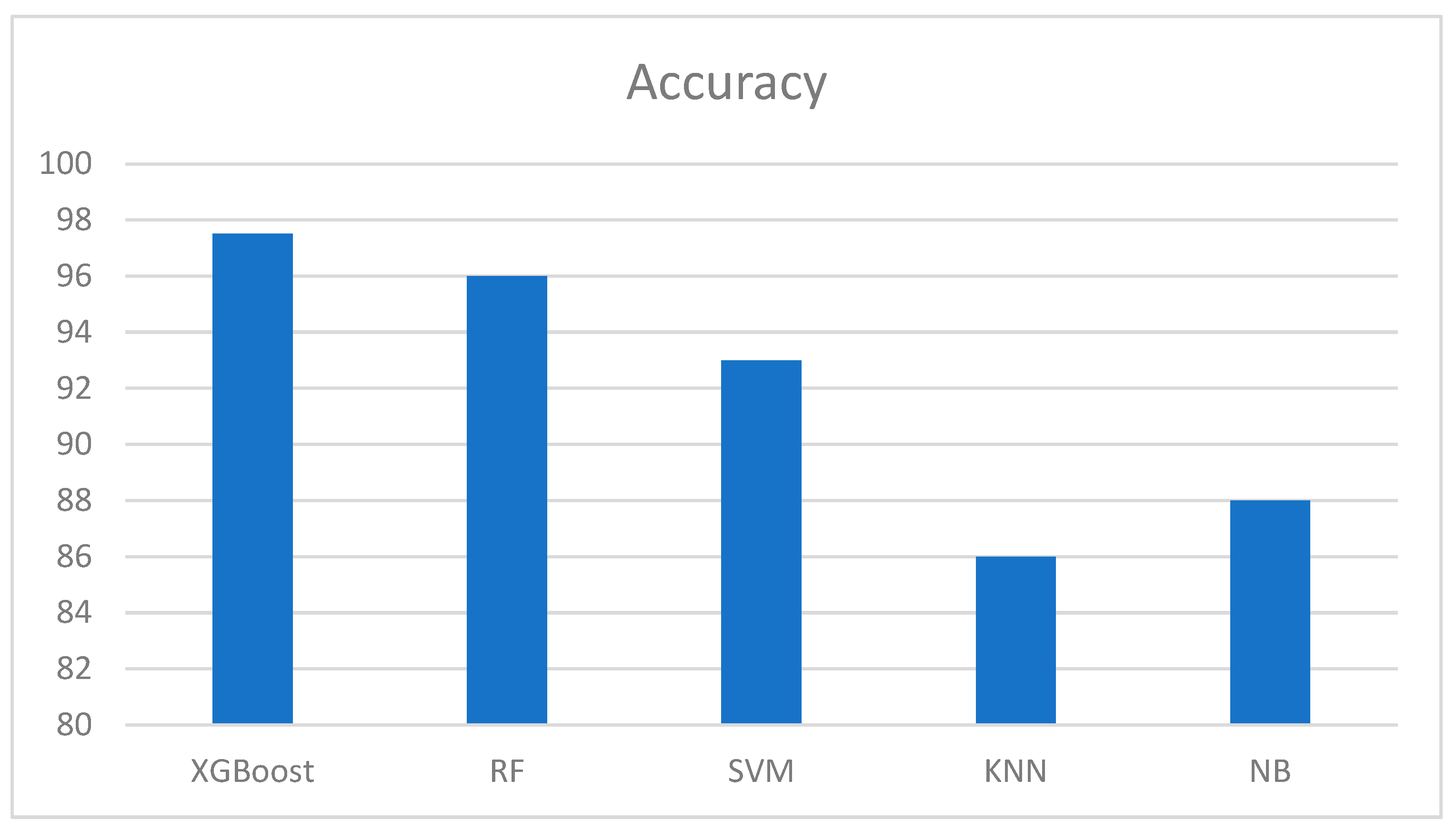
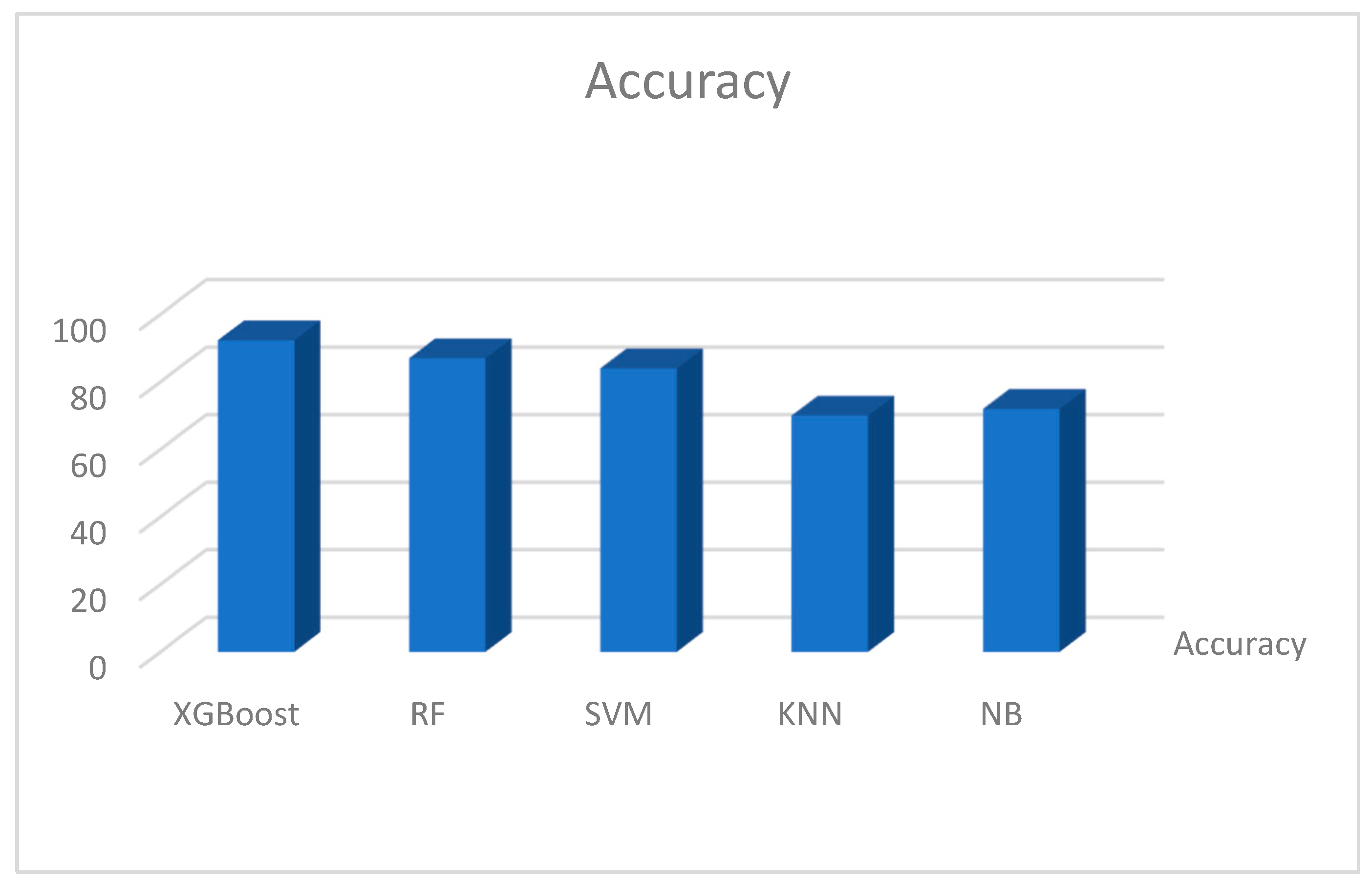
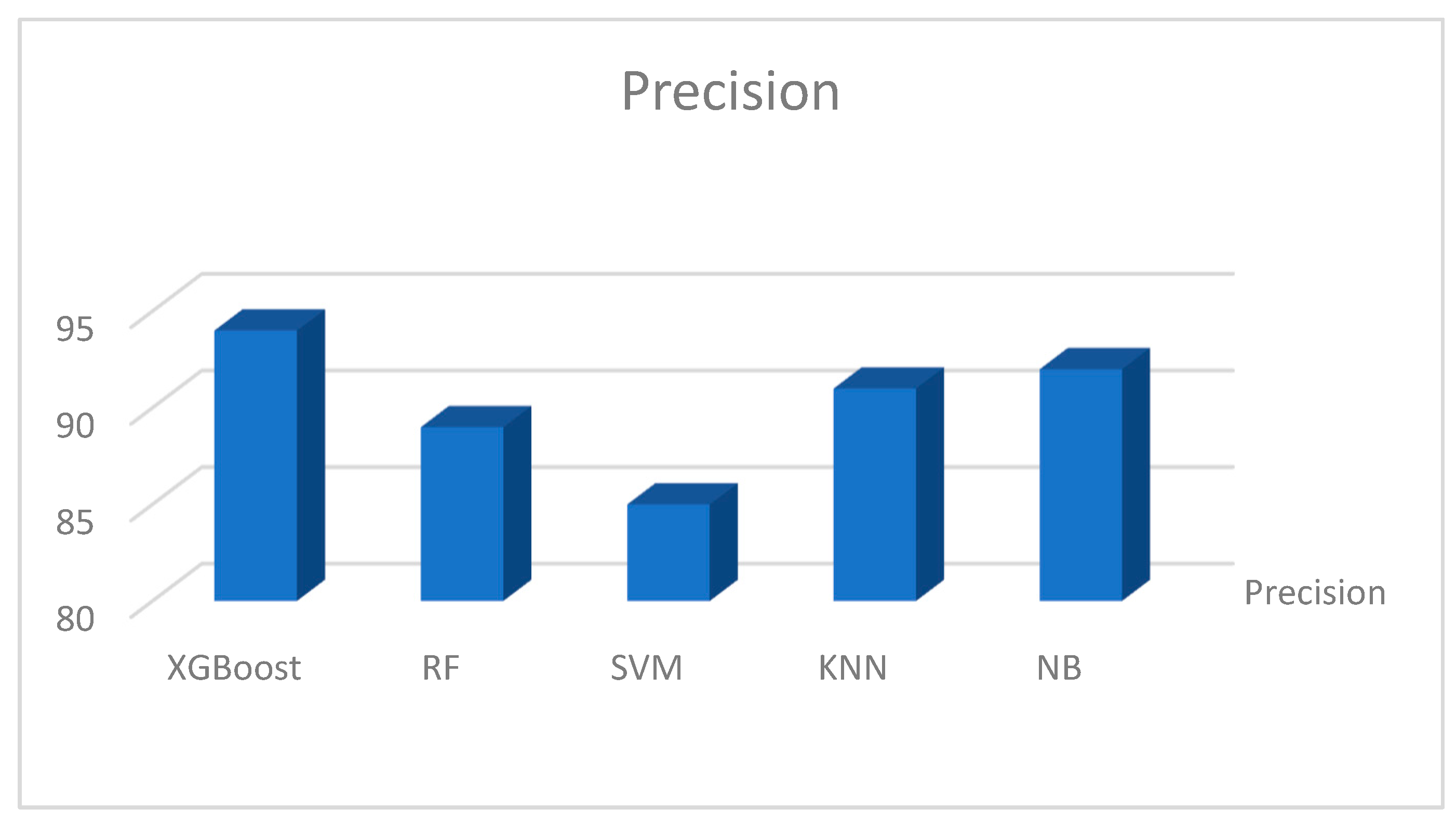
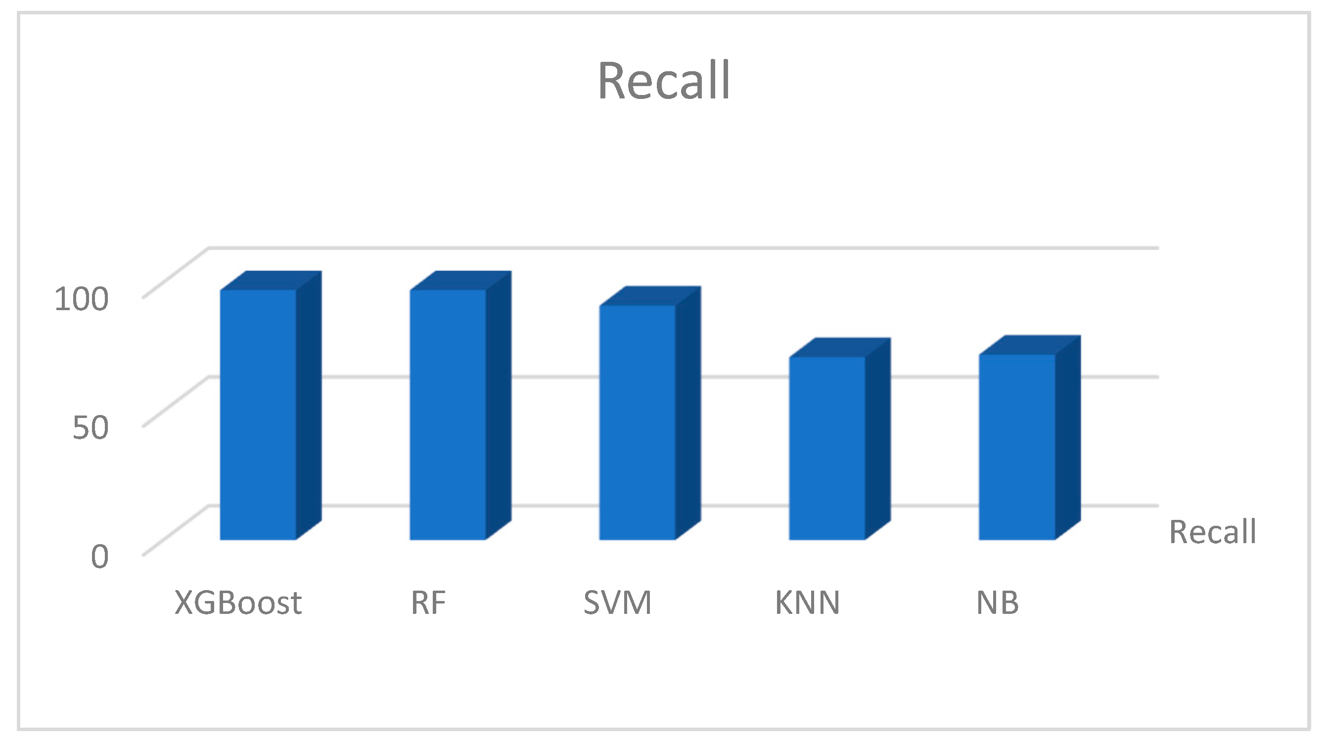
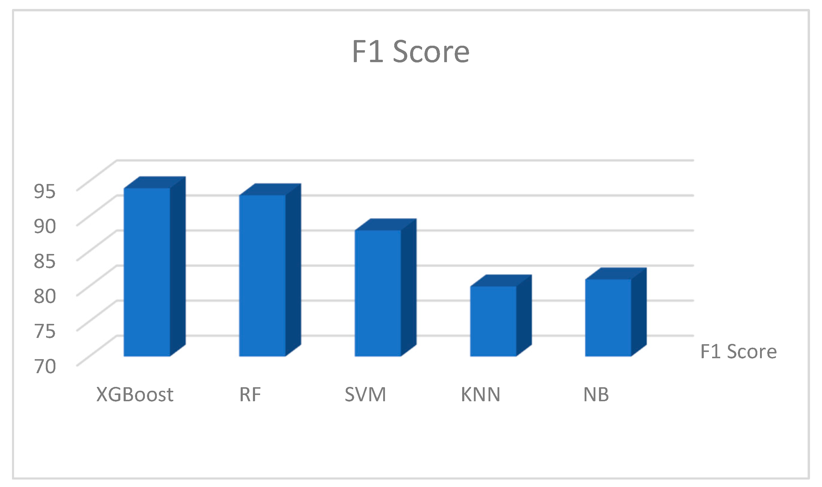
Figure 11 show the outcomes of the evaluation metrics used to further evaluate the performance of the models. It can be observed that the proposed methodology and XGBoost model outperformed all other models used in the previous studies. In
Figure 8, we can observe that XGBoost has the highest accuracy score, followed by the RF and SVM algorithms. XGBoost obtained a precision of 98 %, 100 % recall, and an excellent f1-score. The percentage of accurate predictions in each class was computed using the average recall. In addition, the accuracy of the forecasts was computed, which established confidence in a specific forecast. Moreover, average precision was computed for evaluation purposes, allowing us to determine the average of all precision ratings for each class. Finally, the f1-score was computed, which provided a weighted average of the precision and recall of each class. The score for each sample in a class that is incorrectly predicted was penalized.
5.2. The Kaggle Parkinson’s Disease Dataset
Table 3 presents a comparative analysis of the multiple classifiers on the Kaggle dataset. To evaluate the performance of the supervised machine learning models further, a similar dataset was obtained from the Kaggle machine learning dataset repository to ensure the accuracy of the detection models. The same experimental procedure as that for the UCI dataset was followed. The algorithms did not perform better on this dataset, despite following the pre-processing and feature extraction processes. The models performed better on the UCI dataset than on the dataset provided by Kaggle [
17,
18]. However, one thing that is certain is that the individual model maintains its position; for example, XGBoost has the best performance in both datasets, even though it was 98% and 92% in the UCI and Kaggle datasets, respectively. Similarly, for the other models.
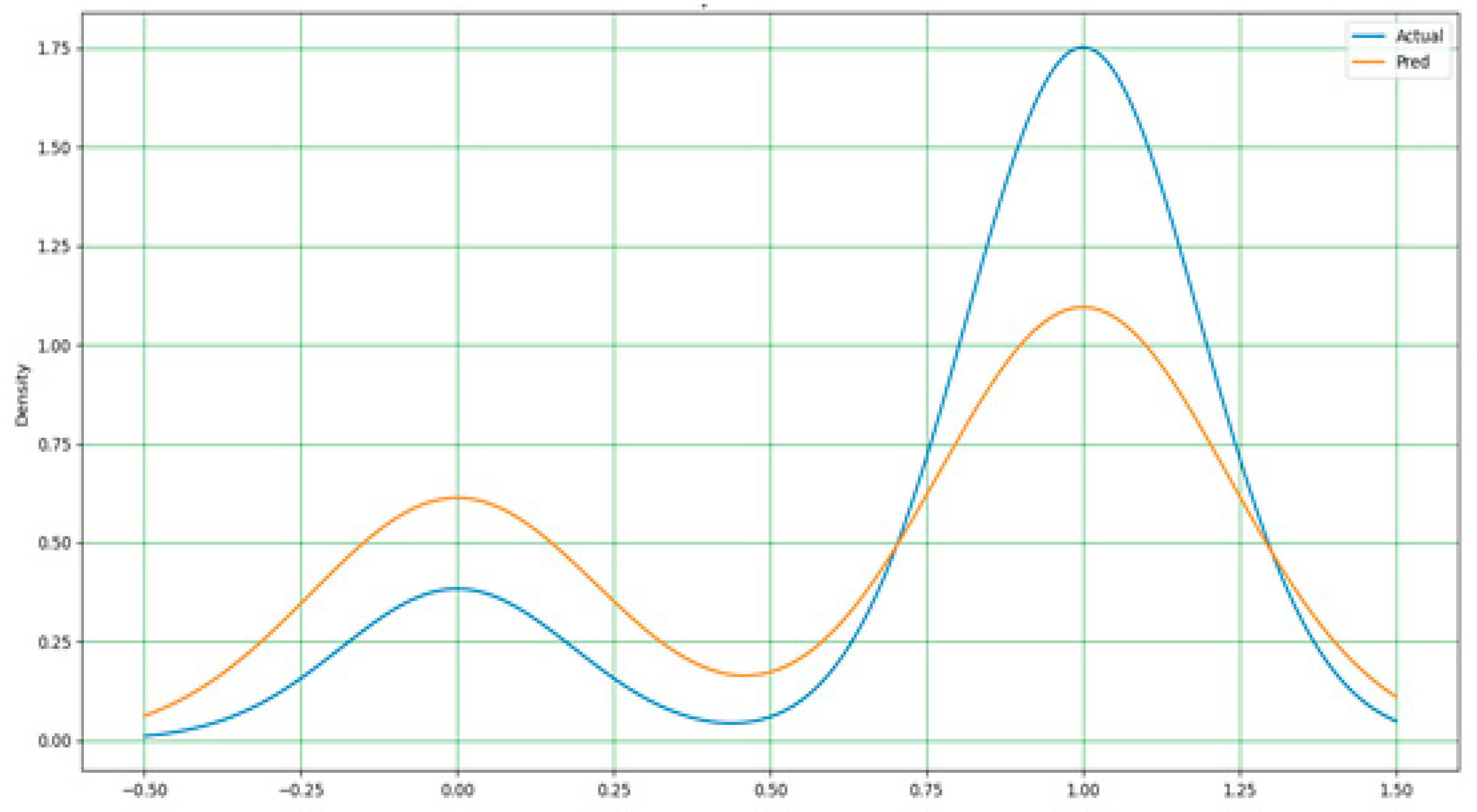
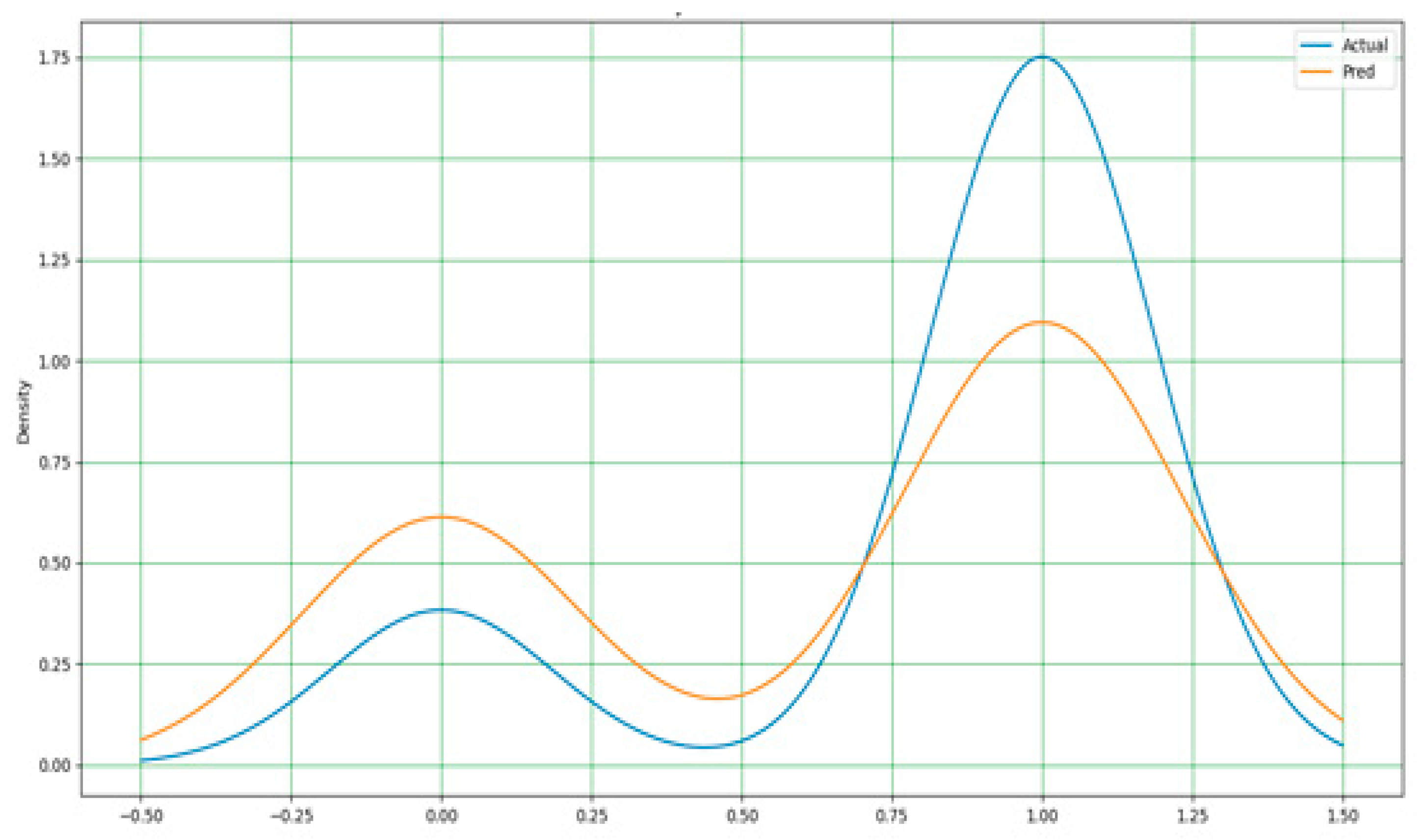
In
Figure 12,
Figure 13 and
Figure 14, a line-type plot was used to plot the actual versus predicted values. The blue lines indicate the actual values of the dataset and the orange lines represent the prediction results.
Figure 12 shows a comparison of the naïve Bayes prediction results with actual data. The performance of the actual and predicted values can be observed clearly, with too many differences between the actual and predicted values. For the random forest in
Figure 13, the difference between the actual and predicted is not as clear as that in naïve Bayes, but there is some way to go to obtain an accurate prediction.
As stated earlier, the extreme gradient boost in
Figure 14 outperformed all models in terms of performance accuracy and other evaluation metrics. It has a nearly perfect prediction, and the difference between the actual and predicted values is very minimal. Hence, a simple adjustment is required to achieve a perfect output of 100%.
Figure 15 and
Figure 16 display the actual and predicted performances of support vector machine and k-nearest neighbors, respectively.
Figure 17,
Figure 18,
Figure 19 and
Figure 20 show the individual accuracies of the boosting algorithms used for the study on the Kaggle dataset. The accuracy of the testing dataset was approximately 92% with the extreme gradient boosting model. The two supervised algorithms, RF and SVM achieved accuracies of 87% and 89%, respectively.
Figure 17,
Figure 18,
Figure 19 and
Figure 20 show the detailed results of the combined machine learning algorithm models in terms of accuracy, precision, recall, and f1-score. These findings reveal the capabilities of boosting machine learning algorithms such as XGBoost. The study presents state-of-the-art research findings to academic databases that can be used for reference and both supplementary and advanced studies that should continue to find a cure for the disease, if not eliminate it completely.
6. Conclusion
This study analyzed and evaluated various supervised machine learning models to assess the presence of Parkinson’s disease among individuals. An extreme gradient boosting model, along with other models, such as naïve Bayes, random forest, k-nearest neighbor, and support vector machine, was implemented to determine the best outcome. The XGBoost model is regarded as a powerful boosting machine learning technique, particularly in terms of speed and accuracy. The results obtained showed that the XGBoost model, which is an optimized version of other boosting models, is capable of predicting the presence of Parkinson’s disease with relatively very high accuracy compared to other algorithms. The implemented classification algorithm based on the extreme gradient boosting method achieved approximately 98 % accuracy, 97.5 % precision, 100.0 % recall, and 98.7 % f1-score which is a high performance compared to Milano et al., [
20] classification accuracy of approximately 93 % using a K-NN classification algorithm, and Aich et al., [
11] who applied naïve Bayes, k-nearest neighbor, support vector machine, and random forest classifiers. It is recommended that the boosting algorithms should be further explored to study various areas or experiments as it has the potential to outperform other popular and commonly used machine learning classifiers.
Author Contributions
Conceptualization, S.A. and S. I.; data curation, S. A. S. I.., J.-A.L., and S. B.; formal analysis: S.A., S. I., J.-A.L., and S. B.; funding acquisition: J.-A.L.; investigation: S.A. and S. I.; methodology: S.A. and S. I.., S. B.; Project administration, J.-A.L. and S. B.; Resources, S.A. and S.I.; Software, S.A. and S. I.; Supervision, J.-A.L. and S. B.; Validation, S.A., S. I., J.-A.L., and S. B.; Visualization, J.-A.L. and S. A.; Writing—original draft, S.A.; Writing—review and editing, J.-A.L. and S. B.
Funding
This research was supported by the Basic Science Research Program through the National Research Foundation of Korea (NRF), funded by the Ministry of Education (2019R1I1A3A01058887) and, in part, by the Korea Institute of Energy Technology Evaluation and Planning and the Ministry of Trade, Industry, and Energy of the Republic of Korea under Grant 20184010201650.
Institutional Review Board Statement
Not applicable.
Informed Consent Statement
Not applicable.
Data Availability Statement
Acknowledgments
The authors would like to thank the National Research Foundation of Korea through the Ministry of ICT, the Korea Institute of Energy Evaluation and Planning, and the Ministry of Trade, Industry, and Energy of the Republic of Korea for providing financial support for this research work.
Conflicts of Interest
The authors declare no conflicts of interest.
References
- Chintalapudi, N., Battineni, G., Hossain, M. A., and Amenta, F. Cascaded Deep Learning Frameworks in Contribution to the Detection of Parkinson’s Disease. Bioengineering 2022, 9, 116. [CrossRef]
- Borzì, L., Mazzetta, I., Zampogna, A., Suppa, A.; Olmo, G., Irrera, F. Prediction of Freezing of Gait in Parkinson’s Disease Using Wearables and Machine Learning. Sensors 2021, 21, 614. [CrossRef]
- Aljalal, M., Aldosari, S.A., AlSharabi, K., Abdurraqeeb, A.M., Alturki, F.A. Parkinson’s Disease Detection from Resting-State EEG Signals Using Common Spatial Pattern, Entropy, and Machine Learning Techniques. Diagnostics 2022, 12, 1033.
- Hoq, M.; Uddin, M.N.; Park, S.-B. Vocal Feature Extraction-Based Artificial Intelligent Model for Parkinson’s Disease Detection. Diagnostics, 11, 1076. [CrossRef]
- Kurmi, A., Biswas, S., Sen, S., Sinitca, A., Kaplun, D., Sarkar, R. An Ensemble of CNN Models for Parkinson’s Disease Detection Using DaTscan Images. Diagnostics 2022, 12, 1173. [CrossRef]
- Fujita, T., Luo, Z., Quan, C., Mori, K., Cao, S. Performance Evaluation of RNN with Hyperbolic Secant in Gate Structure through Application of Parkinson’s Disease Detection. Appl. Sci., 11, 4361. [CrossRef]
- Mei J, Desrosiers C, and Frasnelli J. Machine Learning for the Diagnosis of Parkinson’s Disease: A Review of Literature. Front. Aging Neurosci. 13:633752. [CrossRef]
- How, M., Uddin, M.N., Park, S.-B. Vocal Feature Extraction-Based Artificial Intelligent Model for Parkinson’s Disease Detection. Diagnostics 2021, 11, 1076. [CrossRef]
- Byeon, H. Application of Machine Learning Technique to Distinguish Parkinson’s Disease Dementia and Alzheimer’s Dementia: Predictive Power of Parkinson’s Disease-Related Non-Motor Symptoms and Neuropsychological Profile. J. Pers. Med. 2020, 10, 31;. [CrossRef]
- Ozkan, H. A Comparison of Classification Methods for Telediagnosis of Parkinson’s Disease. Entropy 2016, 18, 115;. [CrossRef]
- Aich, S., Youn, J., Chakraborty, S., Pradhan, P. M., Park, J., Park, S., and Park, J. A Supervised Machine Learning Approach to Detect the On/Off State in Parkinson’s Disease Using Wearable Based Gait Signals. Diagnostics 2020, 10, 421;.
- Demir, F., Siddique, K., Alswaitti, M., Demir, K.; Sengur, A. A. Simple and Effective Approach Based on a Multi-Level Feature Selection for Automated Parkinson’s Disease Detection. J. Pers. Med. 2022, 12, 55. [CrossRef]
- Alzubaidi, M.S., Shah, U., Dhia Zubaydi, H., Dolaat, K., Abd-Alrazaq, A.A., Ahmed, A., Househ, M. (2021). The Role of Neural Network for the Detection of Parkinson’s Disease: A Scoping Review. Healthcare, 9, 740. [CrossRef]
- Bae, D.-J., Kwon, B.-S., Song, K.-B. XGBoost-BasedDay-Ahead Load Forecasting Algorithm Considering Behind-the-Meter Solar PV Generation. Energies, 15, 128. [CrossRef]
- Williamson, J.R., Telfer, B., Mullany, R., Friedl, K.E. Detecting Parkinson’s Disease from Wrist-Worn Accelerometry in the U.K. Biobank. Sensors, 21, 2047. [CrossRef]
- Pramanik, M., Pradhan, R., Nandy, P., & Bhoi, A. K. Applied Sciences Machine Learning Methods With Decision Forests For Parkinson ’ S Detection. Appl. Sci. 2021, 11, 581.
- https://archive.ics.uci.edu/ml/datasets accessed on 4th August, 2023.
- https://www.kaggle.com/datasets accessed on 4th August, 2023.
- Gil-Martín, M., Montero, J. M., and San-Segundo, R. Parkinson’s Disease Detection from Drawing Movements Using Convolutional Neural Networks, Electronics 2019, 8, 907;.
- https://numpy.org accessed on 4th August, 2023.
- https://pandas.pydata.org accessed on 4th August, 2023.
- https://jupyter.org/ accessed on 4th August, 2023.
- https://scikit-learn.org accessed on 4th August, 2023.
- Milano, F., Cerro, G., Santoni, F., De Angelis, A., Miele, G., Rodio, A., Moschitta, A., Ferrigno, L., Carbone, P. Parkinson’s Disease Patient Monitoring: A Real-Time Tracking and Tremor Detection System Based on Magnetic Measurements. Sensors 2021, 21, 4196.
- Pardoel, S., Kofman, J., Nantel, J., and Lemaire, E. D. Wearable-Sensor-Based Detection and Prediction of Freezing of Gait in Parkinson’s Disease: A Review. Sensors 2019, 19, 5141;. [CrossRef]
- Rich, S., Youn, J., Chakraborty, S., Pradhan, P. M., Park, J., Park, S., and Park J. A Supervised Machine Learning Approach to Detect the On/OFF State in Parkinson’s Disease Using Wearable Based Gait Signals. Diagnostics 2020, 10, 421;. [CrossRef]
- Chollette C. Olisah, Lyndon Smith, Melvyn Smith. Diabetes mellitus prediction and diagnosis from a data preprocessing and machine learning perspective, Computer Methods and Programs in Biomedicine,Volume 220, 2022, 106773, ISSN 0169-2607. [CrossRef]
- Pianpanit, T., Lolak, S., Sawangjai, P., Sudhawiyangkul, T. and Wilaiprasitporn, T. Parkinson’s Disease Recognition Using SPECT Image and Interpretable AI: A Tutorial. IEEE Sensors Journal.
- Sani Abba, Souley Boukari, Mohammed Ajuji and Amina Nuhu Muhammad, Performance Evaluation and Analysis of Supervised Machine Learning Algorithms for Bitcoin Cryptocurrency Price Forecast, International Journal of Computer Science and Security (IJCSS), Volume 16, Issue 3, 2022, pp. 1-15. https://www.cscjournals.org/library/manuscriptinfo.php?mc=IJCSS-1664.
- Karl Gardner, Rutwik Joshi, Md Nayeem Hasan Kashem, Thanh Quang Pham, Qiugang Lu, Wei Li; Label-free identification of different cancer cells using deep learning-based image analysis. APL Mach. Learn. 1 June 2023; 1 (2): 026110. [CrossRef]
- Y. Belotti, D. S. Jokhun, V. L. M. Valerio, T. W. Chong, C. T. Lim. Deep convolutional neural network accurately classifies different types of bladder cancer cells based on their pH fingerprints and morphology. AIP Advances 1 May 2023; 13 (5): 055325. [CrossRef]
- Alemayehu Getahun Kumela, Abebe Belay Gemta, Alemu Kebede Hordofa, Habtamu Dagnaw, Umer Sheferedin, Mulugeta Tadesse; Quantum machine learning assisted lung cancer telemedicine. AIP Advances 1 July 2023; 13 (7): 075301. [CrossRef]
- Zhiqiang Zheng, Zhichao Chen, Yonghua Lin, Jianfeng Wei; Identification and gene expression analysis of circulating tumor cells with high expression of KRAS in pancreatic cancer. AIP Advances 1 September 2023; 13 (9): 095015. [CrossRef]
|
Disclaimer/Publisher’s Note: The statements, opinions and data contained in all publications are solely those of the individual author(s) and contributor(s) and not of MDPI and/or the editor(s). MDPI and/or the editor(s) disclaim responsibility for any injury to people or property resulting from any ideas, methods, instructions or products referred to in the content. |
© 2023 by the authors. Licensee MDPI, Basel, Switzerland. This article is an open access article distributed under the terms and conditions of the Creative Commons Attribution (CC BY) license (http://creativecommons.org/licenses/by/4.0/).
