1. Introduction
Data-driven methodologies in the field of structural health monitoring (SHM) have seen significant success in a wide range of applications, including damage detection, localization and quantification. The data-based SHM system uses machine learning (ML) or pattern recognition techniques or statistical technique to identify structural conditions based on observed data [
1,
2]. By extracting meaningful patterns and knowledge from large datasets, data mining enables improved damage detection, diagnosis, prognosis and decision-making in SHM systems. Over the last three decades, numerous data-driven approaches for SHM have been reported for various structures employed in civil, aerospace and mechanical domains using vibration, ultrasonic, electrical and magnetic signal based approaches [
3,
4,
5,
6,
7]. Out of these, vibration and ultrasonic signals have been very commonly used for SHM because of their effectiveness and wider applicability for damage detection in structures[
8,
9]. There are generally two types of Machine Learning (ML) algorithms: supervised learning, unsupervised learning. A supervised-learning approach involves training the learning algorithm with available data and a label. The structure's undamaged or damaged state, the location of the damage, or the severity of the damage are all possible labels in SHM. For the supervised learning approach, all damage severity and locations of interest for a specific structure must be included in the training data set. The unavailability of experimentally recorded data from real structure with all relevant class labels is the main problem with supervised learning. In the absence of experimentally recorded damaged data for any structure, one can also use unsupervised machine learning. However, this model’s limitation is that it can only identify the presence or absence of damage[
10]. The model does not offer any specific damage information, such as damage location or severity. One needs to incorporate supervised learning in SHM in order to perform damage diagnosis at an advanced level.
In the majority of cases, collecting training data for the data-based approach through experiments is not practical due to time and resource constraints. Alternatively, the generation of training data using a physics-based model and testing with experimental data could be an alternative strategy. However, this approach could be problematic because the underlying distribution of data generated from the physics-based model and the actual structure are different for various reasons such as environmental uncertainty in experiment, modelling bias of the physics-based model etc. ML models, whether supervised or unsupervised, are created under the presumption that test and training data come from the same distribution. Generation of practical data through a large number of experiments for the purpose of training an ML model is considered impractical. Due to these issues, data-based approaches are not widely used in SHM. These issues are particularly problematic for supervised learning because it needs labeled damage-state data for all potential damage scenarios. Nevertheless, supervised learning has been used for the past three decades to diagnose damage in SHM [
11,
12]. The development of a model for the diagnosis of damage using a data driven method that trains with data generated by a physics-based model and tests with actual signals captured from a structure by experiments has gained attention in recent years. A strain field monitoring-based diagnostic system has been shown to detect, localize and quantify anomalies in a real crack propagating on an aluminum stiffened skin structure [
13]. Lamb wave signal and numerically-enhanced ML approach has been used for assessment of cracks in plate-like structures [
14]. Lamb wave scattering-based hole-type defect diagnosis has been reported in laminated composites [
15,
16]. Application of domain adaptation has also been reported in SHM [
17]. Combination of simulated and experimental data through deep metric learning based SHM has been reported for guided wave signals [
18]. Application of artificial neural network and Probability Ellipse techniques for Lamb wave-based damage detection has also been reported [
19].
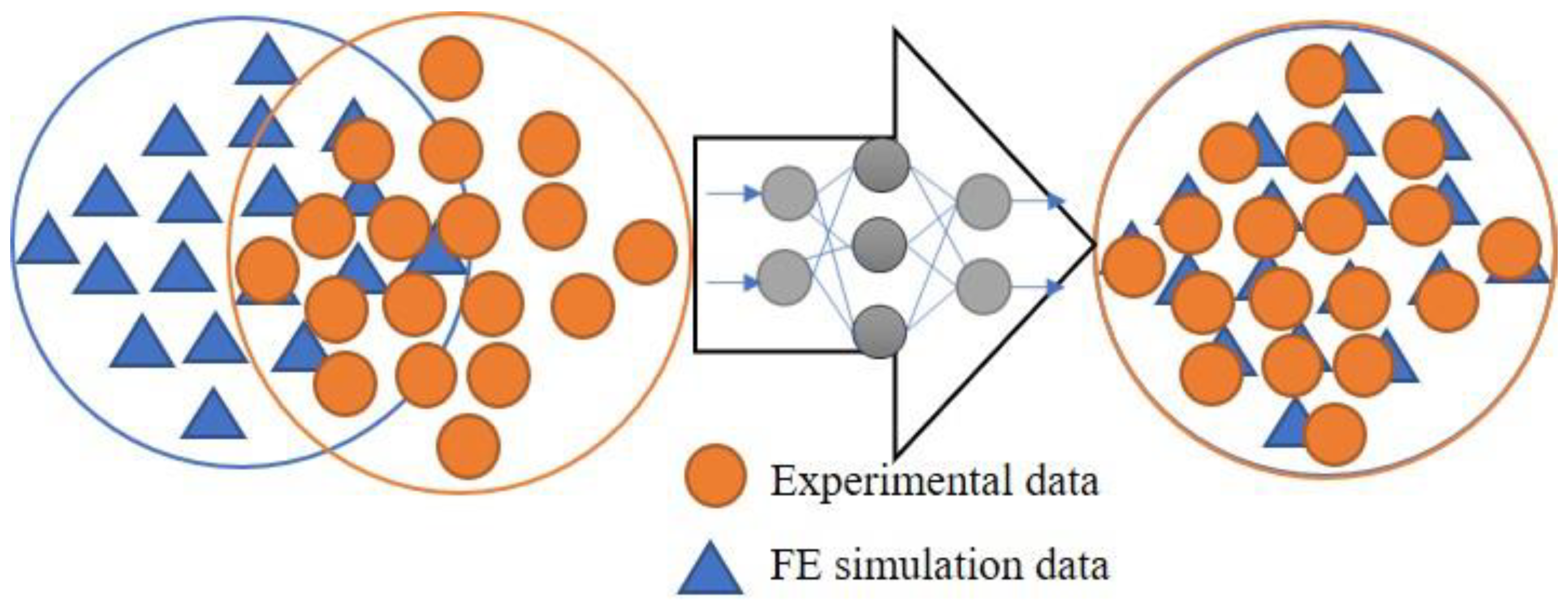
From the study of past work, it is evident that several efforts have been made to mitigate the unavailability of real structure damage data for data-driven SHM. However, most of the study is for guided wave data. There is a clear lack of similar study related to vibrational data-based SHM. In this work, we attempt to fill this lacuna. We report a more generalized methodology than a previously reported work [
20], to reduce the variability between numerically simulated data and experimental data, so that one can generate training data by numerical simulation. In the proposed method, numerically simulated data has been transferred to the experimental domain as shown in
Figure 1.
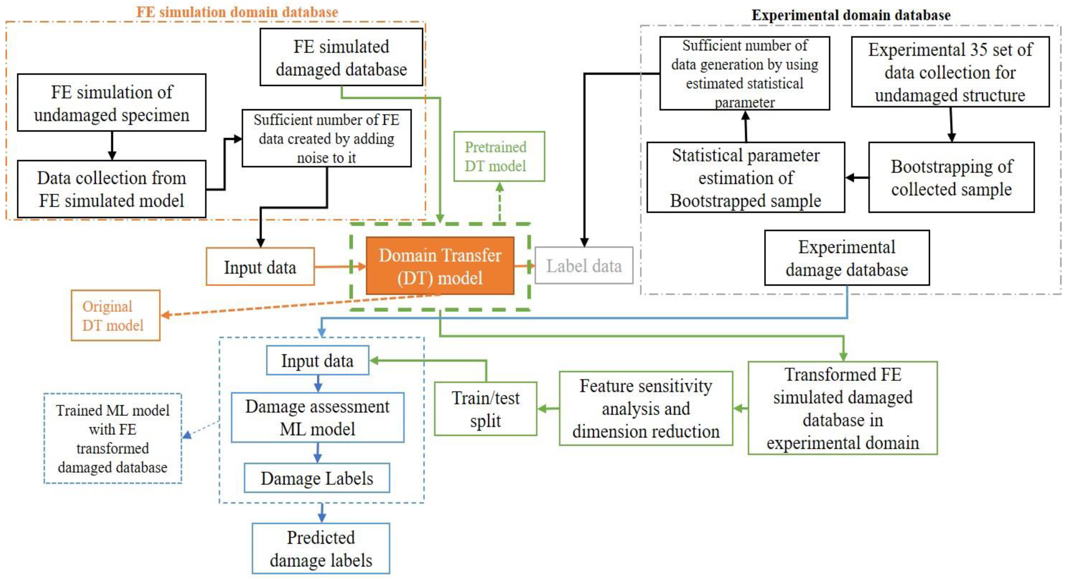
Once the simulated database is transformed to the experimental domain, the transformed dataset is used to train the machine learning model for damage assessment. Thereafter, the trained ML model is used to estimate the damage condition on experimental data. For the domain transformation we have used the artificial neural network (ANN) based deep learning (DL) model and for damage assessment we used a stacked learning model. The proposed methodology is employed to debonding localization and quantification in metallic stiffened panels based on vibration analysis.
The paper is organised in the following sections: In
section 2, the proposed methodology is described; in
section 3, the experimental set-up and specimen details are provided; in
section 4 the Finite Element (FE) simulation of stiffened panels is described; in
section 5 the detailed implementation of the proposed methodology is discussed;
section 6 gives concluding remarks.
3. Experimental Setup and Specimen Detail
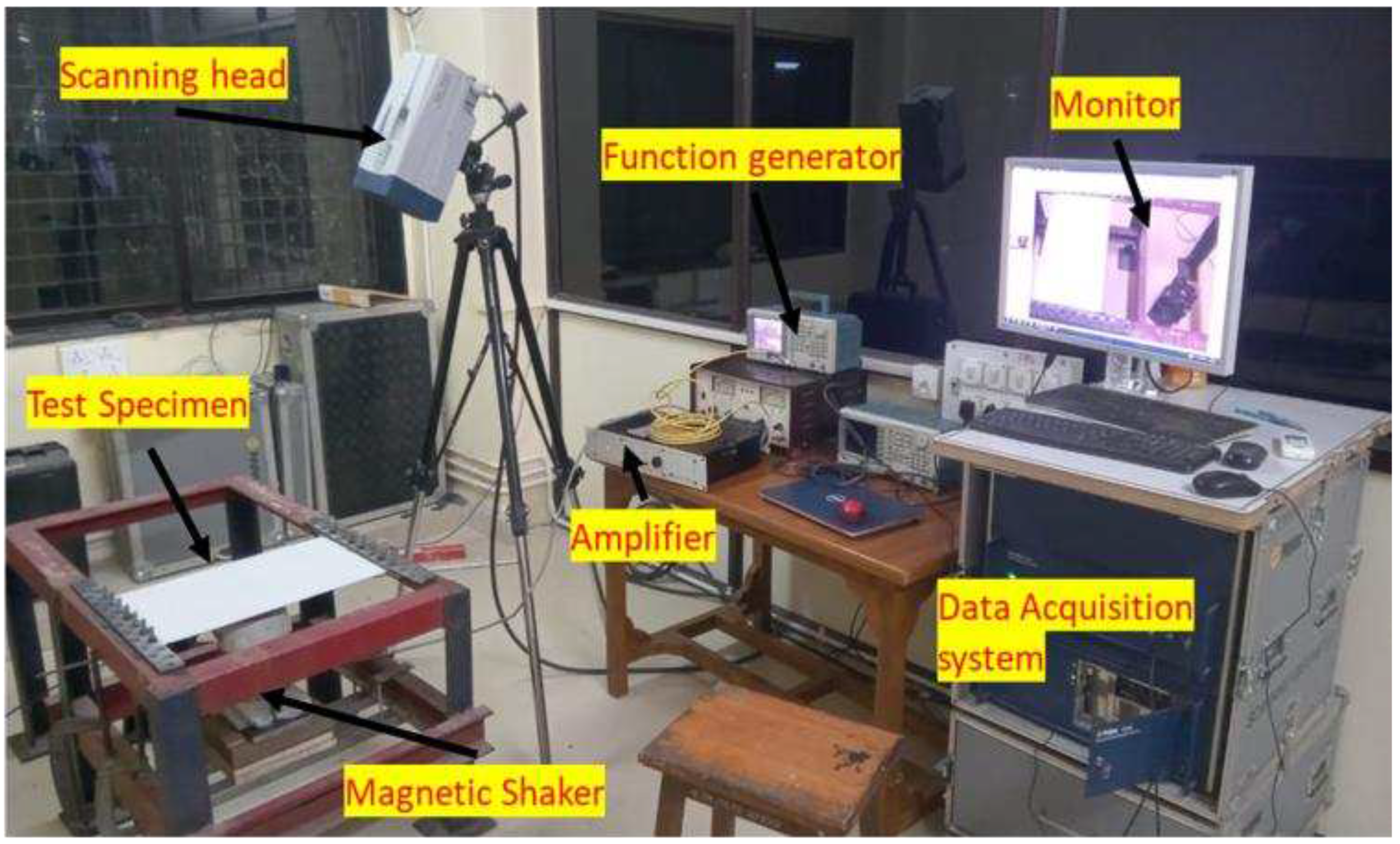
In the present work, a scanning laser doppler vibrometer (LDV) was used to extract vibration data of metallic stiffened panels. The experimental setup for the LDV consists of a laser scanning head PVS 500 linked to a system for data acquisition, an LDS magnetic oscillator V406 M4-CE, a function generator (TEKTRONIX 3021B) and a voltage amplifier (PA100E CE) as shown in
Figure 6.
The experiment was completed in the following sequential steps: positioning of scan head, 2-D alignment, definition of scan points on the specimen, laser focus, scan and data extraction.
3.1. Test Specimen
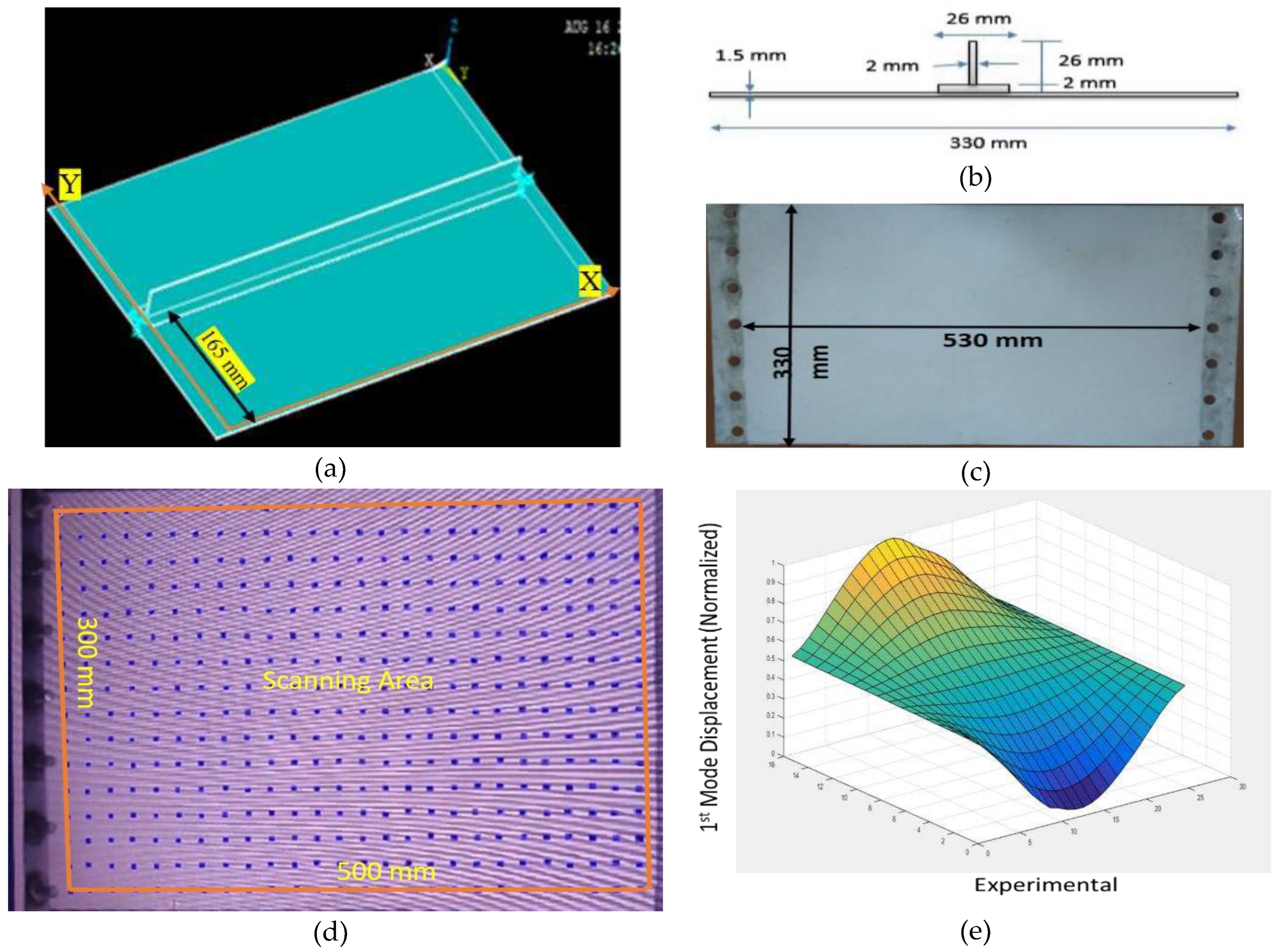
The experiment is carried out on a metallic stiffened panel made of aluminum plate and T-stiffener of material grade AL5052 H32. The dimensions of the plate are 530 mm length, 330 mm width and 1.5 mm thickness and the stiffener has web dimensions of 26 mm × 2 mm and flange dimensions 2 mm × 26 mm. Epoxy adhesive was used to affix the stiffener to the plate. The epoxy adhesive is made by combining resin and hardener in equal amounts (Loctite EA E-102). The bonding-curing time was 24 hours. Four specimens were created, one undamaged and other three damaged (with debonding).
Table 2 shows the locations of the damages.
To improve the laser beam's reflection from the stiffened structure, the plate is painted white (RUST-OLEUM 249126 FLAT WHITE). There were a total of 416 node points, 26 along the length and 16 along the width, with a 20-mm distance between each (
Figure 7). To prevent laser beam scattering, only 300 mm x 500 mm out of 530 mm x 330 mm is taken into account when measuring a point's area as shown in
Figure 7(d). Beyond this area the incident laser might get out of the specimen due bending of the specimen while performing an experiment.
To measure the modal frequency of the experimental specimen, the parameter of LDV were as given in
Table 3:
3.2. Experimental Variability Reduction
One of the most difficult aspects of conducting an experiment is ensuring that the results are consistent with repeat testing of the same specimen or while testing a different specimen. The major source of experimental variability in vibration-based experiments is fixed boundary conditions. Maintaining the same boundary condition for all specimens is nearly impossible. However, keeping equal clamping forces can help minimize the variability of boundary conditions. To accomplish this, at the fixed boundary condition, all clamping nut-and-bolt arrangements were tightened with a torque wrench to a constant torque. The sequence in which the bolts were changed was also considered, with a consistent attachment sequence maintained throughout the test. The mean of 11 tests was used as a single experiment data for each specimen. This was implemented while bootstrapping the original sample data.
4. Numerical Modeling of Stiffened Panel
The finite element software package ANSYS was used to model a stiffened aluminum plate with the same dimensions as the experimental specimen. For the modelling of the plate and stiffener, the eight-noded quadrilateral solid shell element (SOLSH190) with three degrees of freedom in translation direction at each node is used. To determine the size of the element, a convergence analysis was performed and finally meshing of the entire structure was done with 1 mm element size. E = 70.3 GPa, density = 2680 kg/m
3 and Poisson ratio = 0.33 are the mechanical properties of the modelled specimen. Debonding is simulated by breaking the node connection between the plate and stiffener. The contact in the area of debonding is modelled using the parameters in
Table 4.
Numerical Model Verification with Experiment
A numerical model's ability to recreate a real test sample is limited. Nonetheless, certain critical panel parameters can be verified. Important parameters of the vibration-based model are modal frequency and mode shape displacements. However, it is very difficult to verify the mode shape displacements in this specific case of stiffened plate. So, an attempt was made to verify the undamaged specimen's modal frequency. Changing the clamping torque value modifies the fixed boundary condition. This can be done to obtain the modal frequency of an experimental test sample that is close to the numerical model. At a torque of 22 Nm, the experimentally determined first modal frequency showed good agreement with the frequency value predicted by the finite element model, with a difference of 1.17%.
Table 5 shows the first three modal frequencies that were obtained from FE simulated models and experiments on both undamaged and damaged samples.
5. Methodology Implementation
5.1. Data Preparation for Domain Transformation
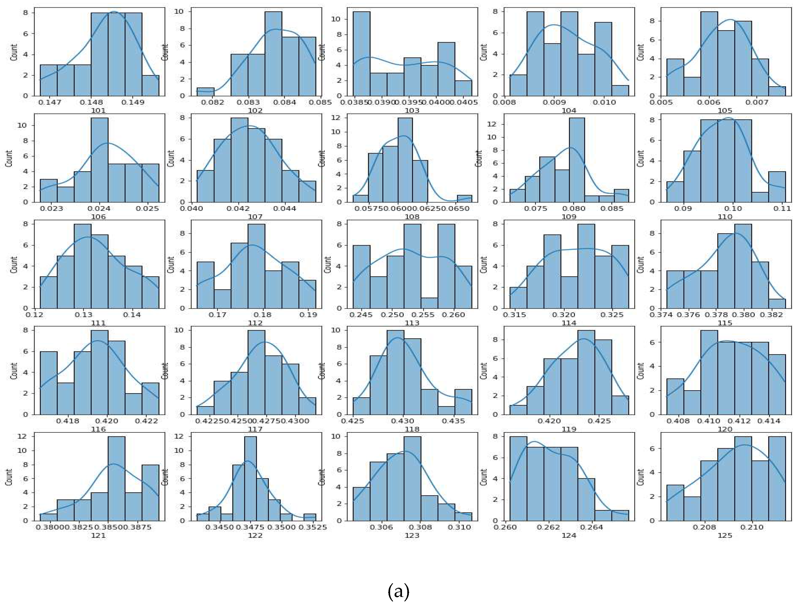
The experimental data pre-processing framework discussed in the methodology section is used to create the experimental dataset for domain transfer. The data preparation started with performing 35 experiments on the LDV experimental set-up to collect 35 samples (as per the central limit theorem, to get better statistical estimation, we require at least 30) of data for each scanning point (shown in
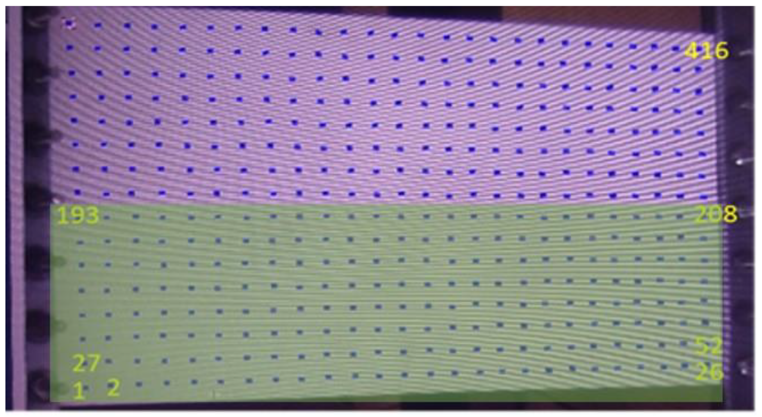
Figure 7(d)) for undamaged stiffened panel. Here, it should be noted that we have a total of 416 scanning points, as shown in
Figure 7(d). Because of the symmetry of the stiffened panel along its length, we only used half of the points, i.e. the first 208 scanning points, in this study, as shown in
Figure 8. The 35 data points were bootstrapped to create a larger sample size of 200. To reduce the experimental variability of experimental data, one bootstrap data is the mean of 11 original collected data, as discussed in
Section 3.2.
Figure 9(a) shows the histogram of the initial 35 data,
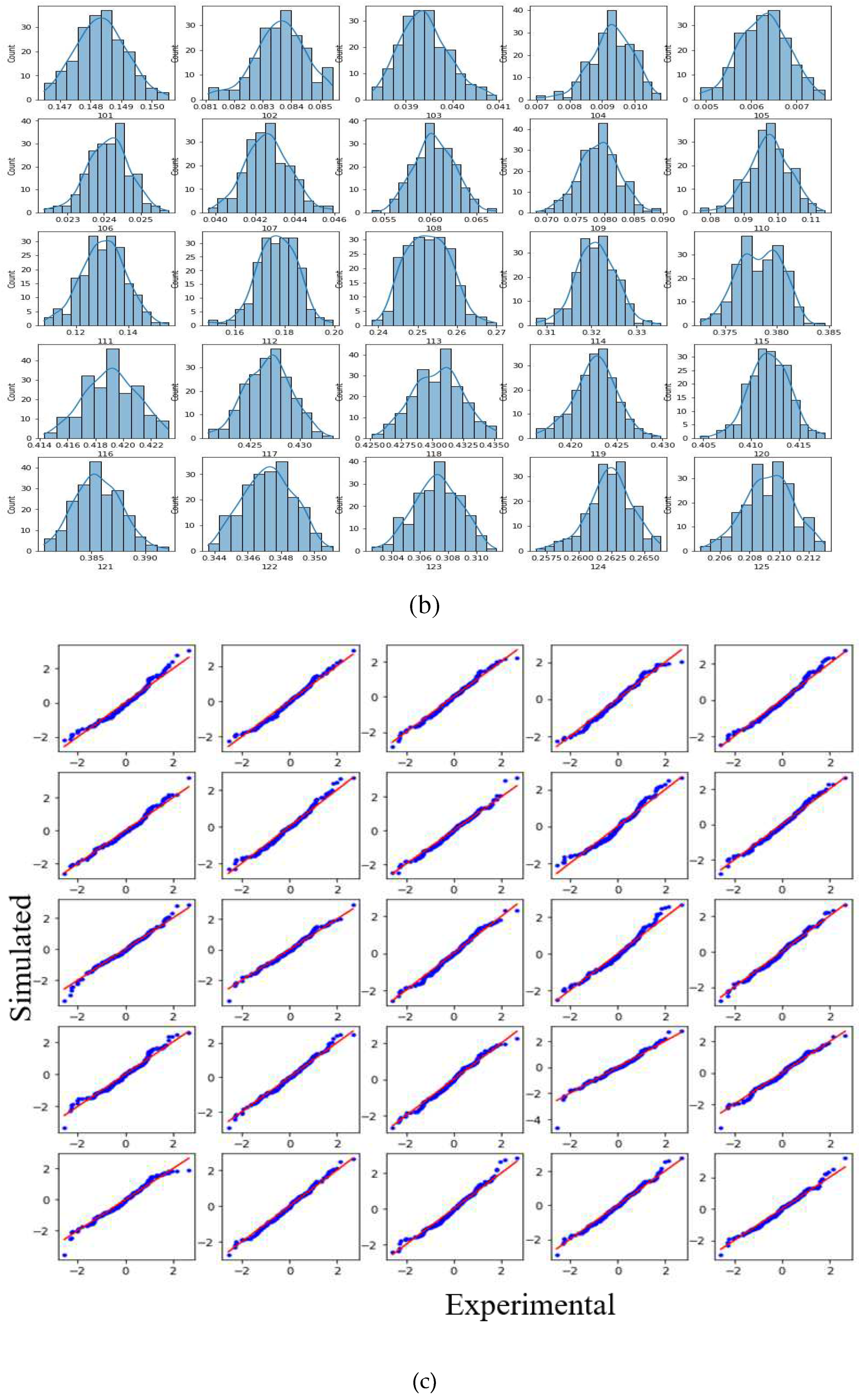
9(b) shows the 200 bootstrapped sample data and
9(c) shows the quantile-quantile (Q-Q) plot for the bootstrap sample data. The Q-Q plot confirms that the bootstrapped data has the same distribution as that of the original sample. Thereafter, the mean and standard deviation (SD) of this sample were calculated and were used with the Python based NumPy library employed to generate a sample of size 1000 for every scan point.
Similarly, we also need 1000 sets of undamaged FE simulated data. In order to create 1000 pieces of data, FE simulated data were repeated 1000 times by adding 0.2 percent random Gaussian noise to them through the Python based NumPy library. Now we have two 1000×208 matrices, one for the undamaged sample experiment and one for the FE simulation of the same.
5.2. Domain Transformation Models
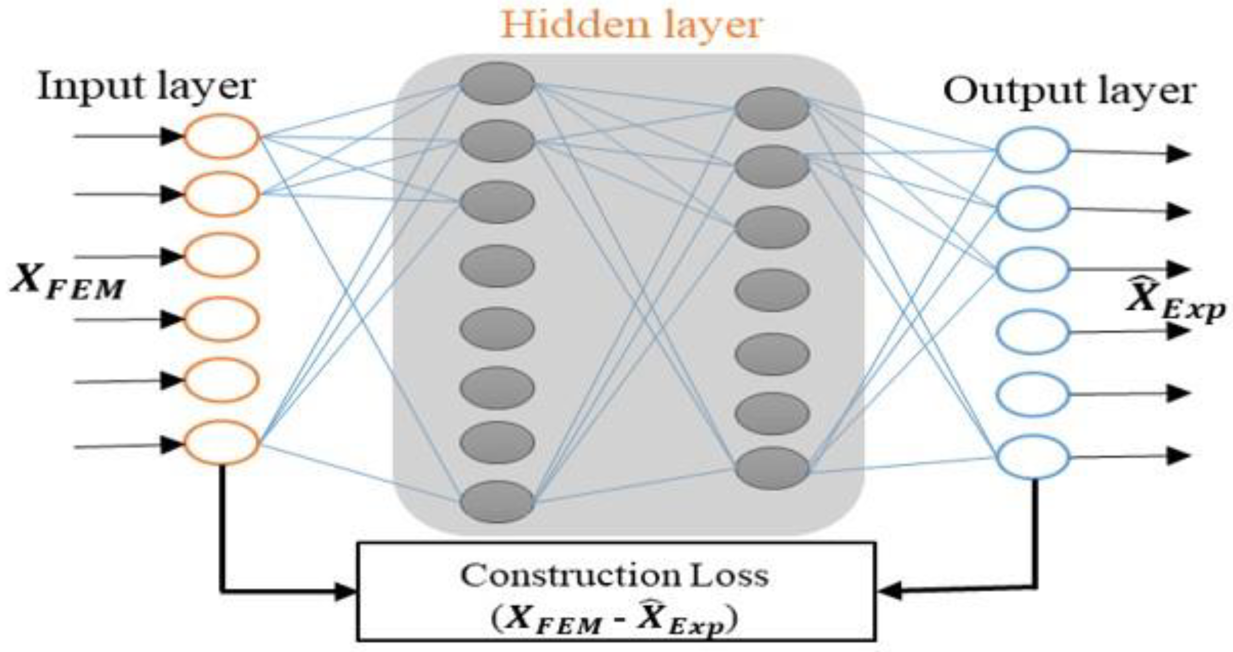
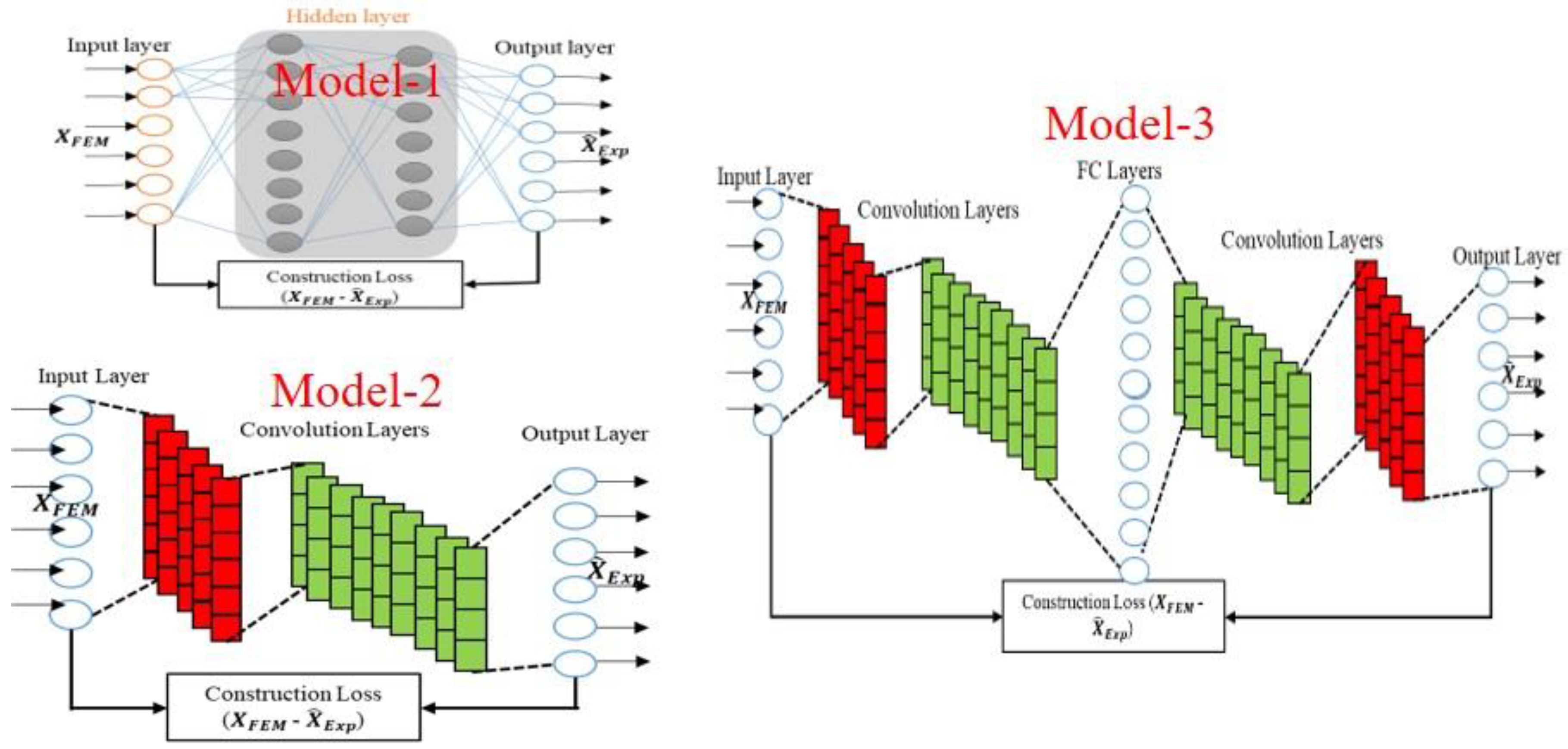
For choosing the appropriate domain transformation model, three neural network-based models were constructed, namely artificial neural network (ANN), a one-dimensional convolution neural network (1D-CNN) and a 1D-CNN plus fully connected network (FC) plus the 1D-CNN (1D-CNN-FC-CNN) as models 1, 2 and 3 respectively. ANNs are computer programmes that work like the neural network in the brain. An ANN is made up of a group of nodes or neurons. Neurons are connected to each other, making a network structure similar to that of the biological neural mechanisms, which is where intelligence comes from. An ANN has a set number of neurons in each layer, input, hidden and output. Mathematically, the ANN for input X and label
can be represented as:
where
is predicted output, X is input vector, W weight, b is bias and
is an activation function.
A loss function compares the target output value and the predicted output value to determine how effectively the ANN models the training data. During training, the goal is to reduce this difference between the predicted and desired outputs as much as possible. The mean square error (MSE) loss function is defined as:
Here L is loss.
The objective of an ANN training algorithm is to minimise the loss function by optimizing the value of weight W and bias b defined as:
Here, J is the Jacobian which optimizes the weight W and bias b to minimise loss L, M is number of samples in training dataset
The 1D-CNN is an effective Deep Learning tool for finding the underlying pattern in a one-dimensional sequence dataset. Several damage detection methods [
31,
32,
33] have used it in different fields. A standard CNN has the following parts: the input layer, convolution layers, a pooling layer and a fully connected layer. Each convolution layer is made up of kernels
k(m) of length
m whose parameters can be learned. Mathematically, the convolution layer for input
x(n) of length n and kernel
k(m) is shown as [
34]:
Here ρ represents the activation function, while the symbol denotes the convolution operation, m is kernel length and n is input length. To obtain an outcome from convolution, a pooling layer is utilized, which extracts inherent signal features.
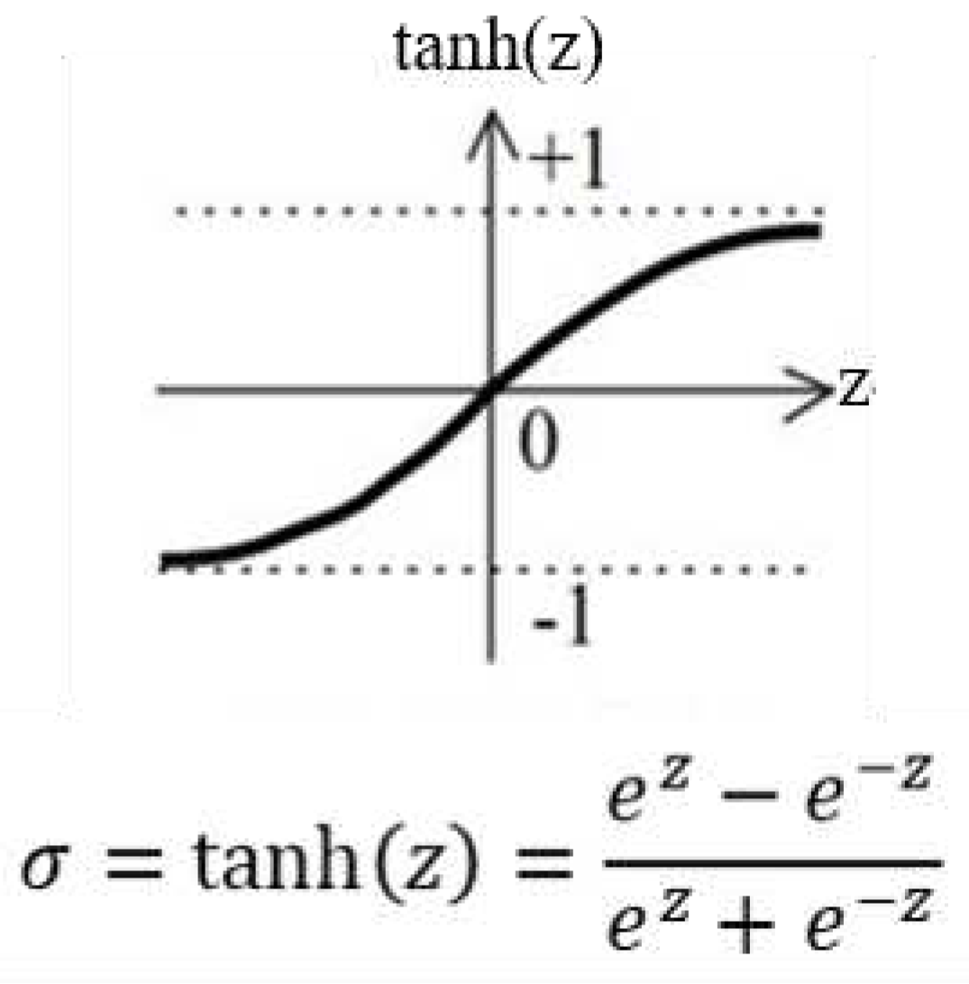
Standard activation functions in ANN architecture are the tangent hyperbolic (tanh), rectified linear unit (ReLU), leaky ReLU and sigmoid. The tangent hyperbolic (
Figure 10) showed better performance in terms of sensitivity and learning speed than the other activation functions in the initial trials. So, we have chosen tanh as the activation function throughout the present study. To further accelerate the training process, batch normalization (BN) is introduced between the CNN layers. The training of deep neural nets is significantly accelerated by BN as it tries to minimize the internal covariate shift. It achieves this by fixing the means and variances of the layer inputs during the normalisation step [
35]. The model's architecture and its parameters is shown in
Figure 11. The details models parameter provided in appendix. The total trainable parameters of the three models are 845520, 2118112 and 2905641 for models 1, 2 and 3 respectively.
Once the domain transformation (DT) models are constructed, the next step is the training of the models. The source domain
(input) and target domain
(output) for the DT model are FE simulated database X and an experimental database
, both of size 1000×208. The DT model was trained with the following parameters: batch size of 200, learning rate of 0.0002, MSE loss function and adaptive momentum (Adam) optimizer with weight decay of 1e-5. In order to prevent the problem of overfitting, an early stopping criterion that guarantees generalisation has been adopted [
36]. Pytorch (version 1.11), a deep learning library that is based on Python, is used in both the construction and training of the DT models. The entire process of the methodology pipeline was implemented using local computer with following configuration: device type: CPU(4.6GHz), processor- core 6 intel i7 8700, memory- 16GB Os-Windows10.
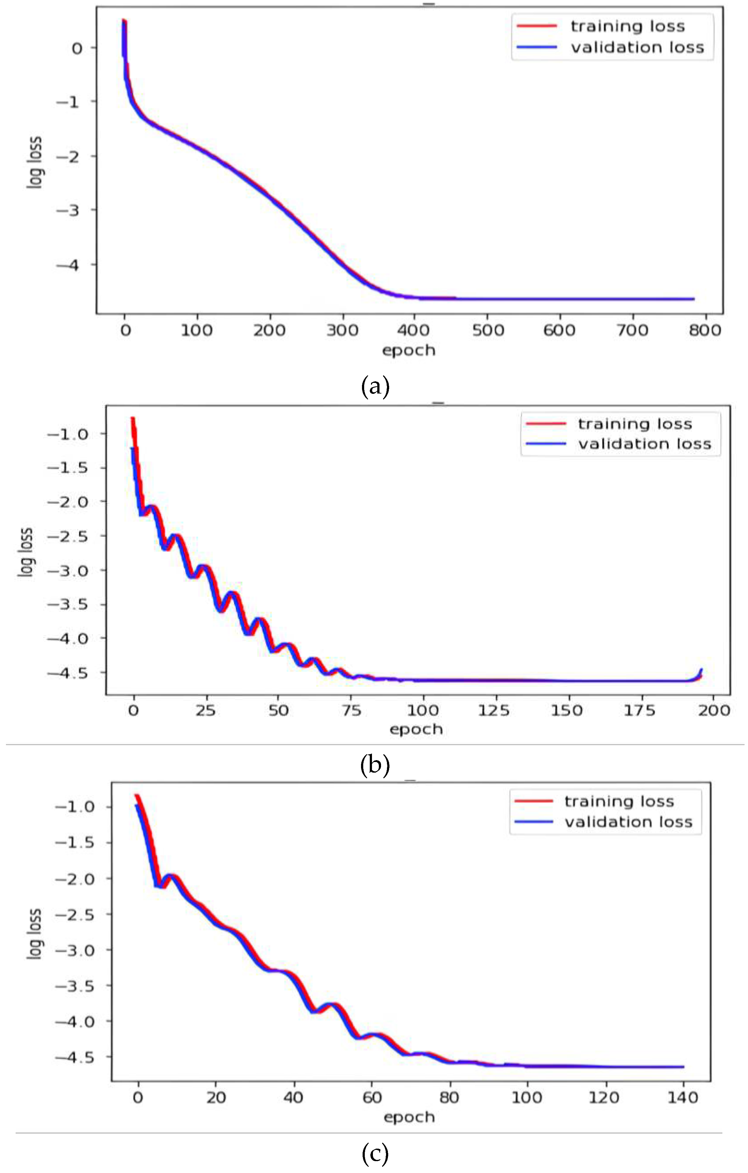
Figure 12 shows the training progress of the DT models.
5.3. Comparison of DT Models
After the DT model construction and training, the performance of the models was compared. There are two relevant criteria that were set: the first is how accurately the model transformed the FE-simulated data to the experimental domain, and the second is to check the effectiveness of the transformed dataset. Here, effectiveness is defined as the ability of the transformed dataset to give better prediction accuracy in damage assessment.
The first criterion is evaluated by comparing the average root mean square error (RMSE) between the damaged experimental data and the damaged FE simulation data after transformation for each damaged experimental specimen. The model with the lowest RMSE is considered the best. Here, it is important to mention the experimental damage data preparation procedure. We have collected 15 sets of experimental data for each damaged specimen by performing 15 experiments on the LDV lab setup. Then a similar procedure was followed as in the case of undamaged experimental data pre-processing, as discussed in
Section 5.1. Finally 50 data points were generated for each damaged case.
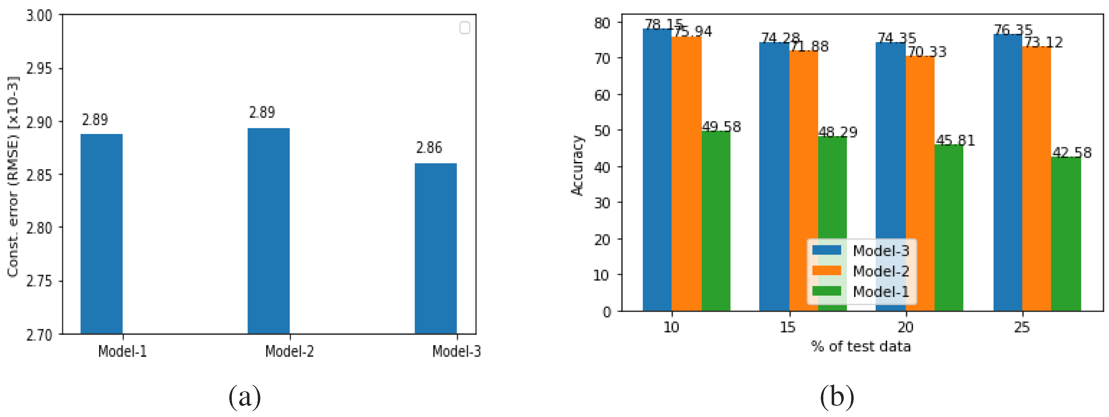
Figure 13(a) shows the average RMSE of the DT models while transforming FE-simulated damaged data to the experimental domain for each experimental damaged data. The figure clearly shows that the DT model 3 produces minimum RMSE in transforming the FE data to the experimental domain.
To check the second criteria i.e. the effectiveness of the transformed dataset, first the FE simulated damage database was transformed into an experimental domain using the DT models. Then feature dimensions of the transformed datasets were reduced using PCA. The number of PCA components was decided by checking the cumulative sum of variance and then using the number of components which capture 98 % variance in the dataset. Then this PCA of transformed dataset was split into training and testing datasets, followed by the training of an ML model with the training dataset and testing with the testing dataset. The target label for damaged location is the debonding zone in stiffened panel.
Table 6 lists the division of debonding zones according to debonding location. Four types of testing were done with the testing dataset being 10, 15, 20 and 25 percent of the original dataset. The ML model used was Support Vector Machine (SVM).
Figure 13 shows the performance of the SVM model in debonding zone identification at various train-test split ratios with the dataset transformed by DT models 1, 2 and 3 respectively. From the figure, it can be seen that SVM gives the best accuracy score for debonding zone identification when the FE data is transformed using DT Model 3.
Based on the two criteria and the respective performances of the DT models to fulfil these criteria, it can be concluded that model 3 is the best choice to proceed with.
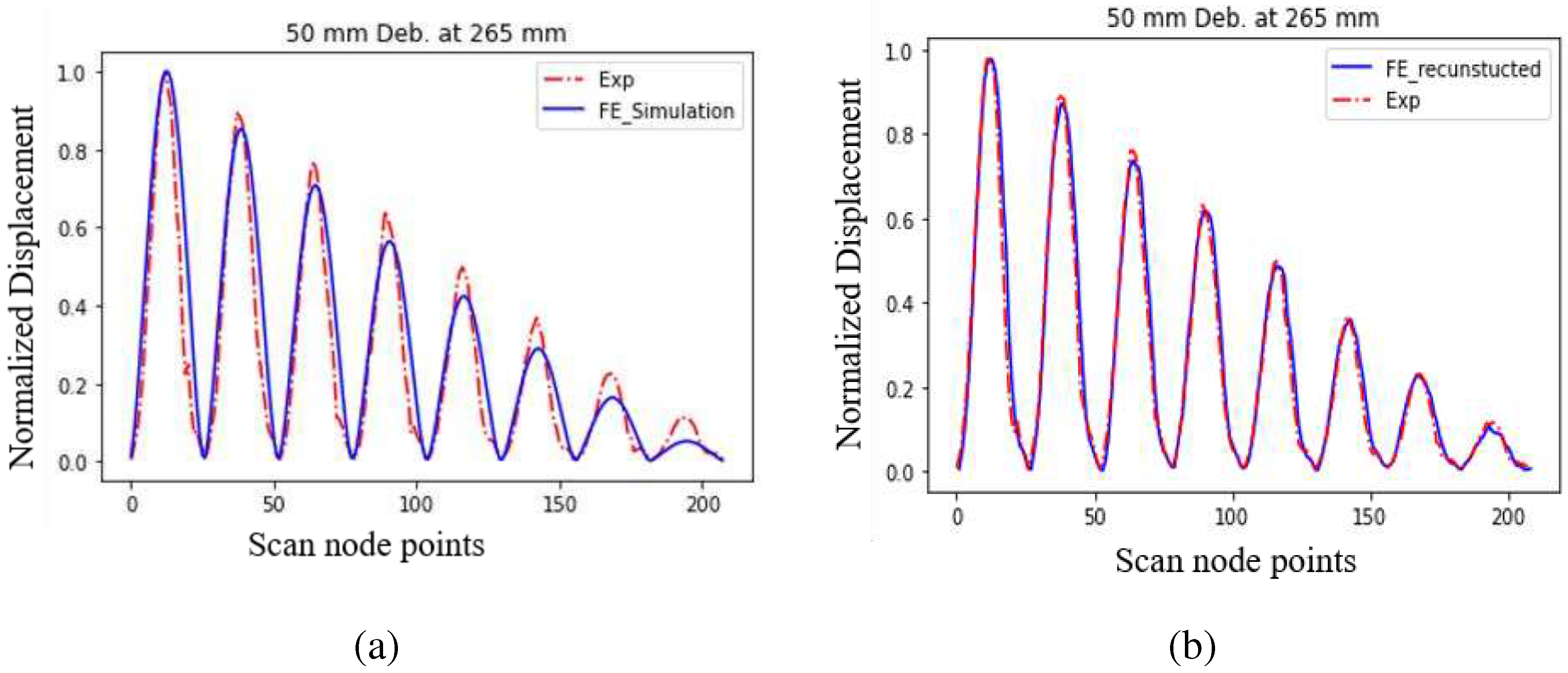
Figure 12(b) also shows that the DT models with more trainable parameters perform better compared to the model with less trainable parameters. The visual comparison between FE simulated and experimental vibration mode shape displacement data for debonding length 50 mm at 265 mm is shown in
Figure 14 (a) before transformation and
Figure 14 (b) after transformation using DT model 3. The figure clearly shows that the transformed FE simulated data is very close to the experimental data.
5.4. Damage Assessment
5.4.1. Feature Sensitivity Analysis
This section discusses the preprocessing of the transformed dataset and the debonding evaluation procedure. The data preprocessing procedure begins with feature-sensitive analysis, also known as feature extraction. The goal of feature extraction is to extract lower-dimensional features and more susceptible-to-damage features from high-dimensional raw data. For the feature extraction process, a procedure based on Mahalanobis Square Distance (MSD) was adopted. MSD is a statistical measure for assessing discrepancy between different datasets. Its use in damage detection is described in detail by Worden et. al. [
37]. The MSD of a multivariate data set consists of n observations in p variables. The MSD is employed to estimate any observed data's discordance. Mathematically, for multivariate data, the MSD is defined as:
where
is the sample mean of observation,
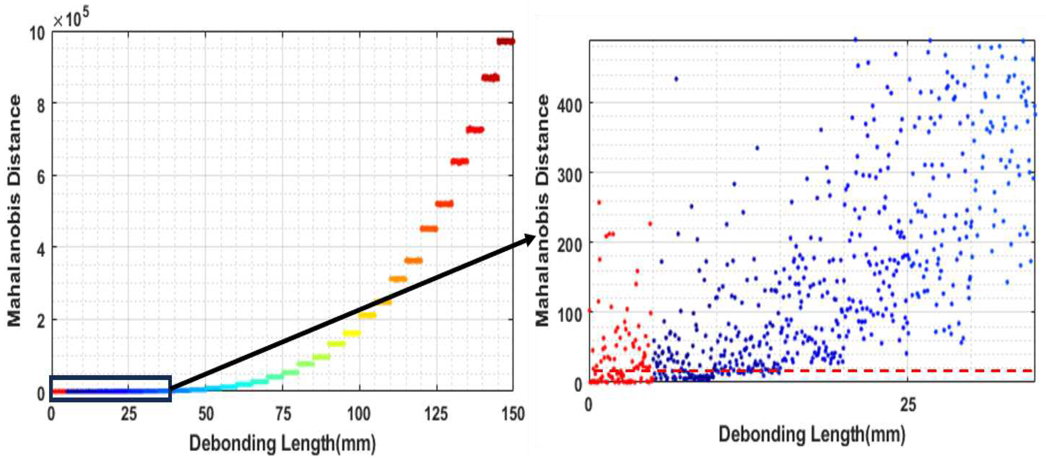
is an outlier, and S is the sample covariance matrix. In our exercise, the MSD estimation started with the creation of 2000 copies of an undamaged dataset by adding 0.2 % of gaussian noise to it. Then MSD was estimated for each damaged case. It was observed that for debonding locations away from the center location (i.e., away from location 265 mm), the MSD value is higher for the same debonding size. The MSD value was lowest for the debonding situated at the center location (at 265 mm). Also, it was observed that the MSD values are monotonically increasing with the size of debonding at the same debonding location. So, to set the threshold limit of the MSD value, it was required to study the MSD value for each debonding size located at the centre (at 265 mm). 100 copies of the dataset for each debonding size were created by adding 0.2 percent of gaussian noise. In
Figure 15, the estimated MSD value for the created dataset is shown for the corresponding debonding size, located at 265 mm. The mean difference between the MSD value for undamaged data and 15 mm of debonding gives a statistically significant result. Therefore, to set the threshold MSD value, 15 mm debonding at the 265 mm location was picked.
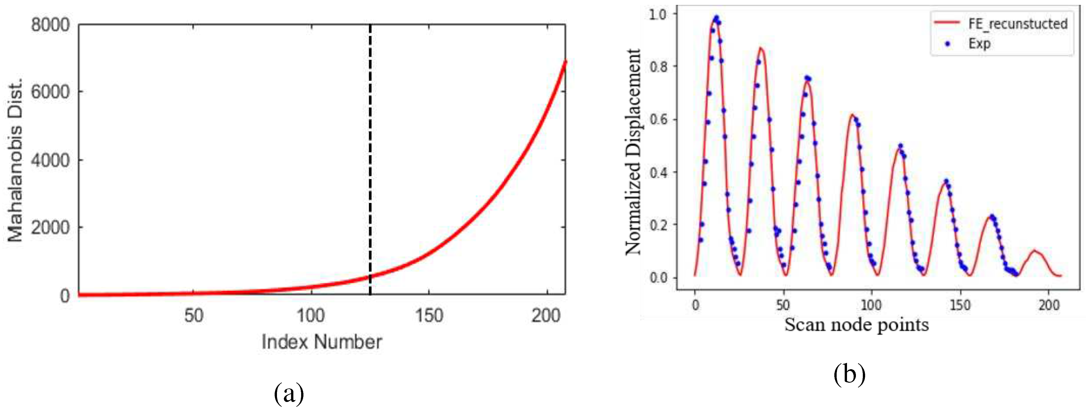
Figure 16 (a) displays the cumulative sum of the calculated MSD for each feature index number for the 15 mm deboning size in ascending order. The threshold MSD value is set as shown in the figure with the vertical line. Thereafter, the MSD value for all feature indices for each debonding case was calculated. Then the calculated MSD was passed through the filter designed according to the threshold MSD value. The feature index number is preserved for values greater than the threshold MSD value. Finally, the set with the preserved index number is selected as the debonding sensitive feature vector. A total of 108 sets of feature index passed the threshold MSD value. Hence the initial feature dimension of size 208 is reduced to 108 after this feature sensitive analysis.
5.4.2. Feature Dimension Reduction
The high dimensional feature vector as an input to ML algorithms frequently results in overfitting and high computational costs, which limits the generalizability of the model. Keeping vital information concerning feature vectors in a lower-dimensional subspace aids in solving these problems. Among the many dimensional reduction techniques available, principal component analysis (PCA) is one that is widely used in ML because it is the most basic and straightforward method of dimensionality reduction. In present study, the first seven PCA components have been used since they are able to cover 98% of total variance in the dataset.
5.4.3. Dataset for Damaged Assessment
A total of 493 damaged cases were modelled in the FE simulation. There are 17 damaged locations ranging from 105 mm to 425 mm along the stiffener length with a step size of 20 mm and at each location, 29 debonding sizes ranging from 10 mm to 150 mm with a step size of 5 mm. These FE datasets were transformed into the experimental domain using the DT model. The transformed FE datasets were used for the training and validation of ML models in damage assessment. Initially, all damage cases were labeled with their corresponding debonding location and debonding size. However, in the initial trial, it was observed that the prediction accuracy for debonding location and size were not reasonable. So, the labels of debonding location and size were changed to debonding location zone and debonding size group.
Table 7 lists the debonding location zones, and
Table 8 lists the debonding size groups.
5.4.4. Performance Evaluation of ML Models in Damage Assessment
The proposed methodology for assessing debonding includes location zone and size group prediction as a classification problem. Five ML algorithms, namely SVM[
38], gradient boosting (GB), random forest (RF) [
39], nearest neighbors classification (K-NN)[
40] and adaptive boosting (ABC) were used as base learning models to a stacked model. The stacked model is an ensemble model that employs a two-stage training procedure. In the initial stage, the base learning model is trained, and in the subsequent stage, the outcome of the base model is used as an input feature for training the meta-model in order to produce the final prediction[
41]. In general, the stacked model approach has been reported to provide better prediction accuracy as compared to base-leaning models[
42,
43,
44,
45,
46].
Two stacked models were created with the same base learner as mentioned above and logistic regression (LR) as a meta-learner (second level learner). One was for debonding location zone prediction and another for debonding size group prediction. They were trained with FE transformed data as input and location zone and size group as targets, respectively. The hyper-parameter of the base learners for the two stacked models were optimized using random grid search algorithms. In random grid search, a predefined range of values for each hyperparameter is specified, and the method picks random combinations of hyperparameters within those ranges for evaluation. The optimal set of hyperparameters is determined by training and evaluating the model for each set of hyperparameters and selecting the combination of parameters that results in the best performance.
Several performance matrices, including accuracy, sensitivity, specivity, F1 score, area under the curve (AUC) of the receiver operating characteristic (ROC) curve, and AUC of the precision recall curve, are commonly used to assess the performance of machine learning models. These performance metrics, however, lack comprehensive information. For instance, the AUC of the precision recall curve and the ROC curve, are excessively broad as they assess all decision criteria, even irrational ones. On the other hand, it is unfair to quantify metrics like accuracy, sensitivity, specificity, positive predictive value, and F1 score at a single threshold that works well in certain situations but not others. To overcome these issue, Carrington et al. 2023 has been proposed a novel performance evaluation technique called deepROC[
47]. The deepROC evaluates performance across several projected risk categories. Deep ROC calculates the averages of sensitivity, specificity, positive and negative predictive values, and likelihood ratios (both positive and negative) for each group as well as the group AUC and the normalized group AUC. In-depth information by group is provided by the deep ROC analysis, which often enhances model assessment over the regular ROC. For further information, readers are suggested to look up the work of Corrington et al. (2020) and Corrington et al. (2023). In present study we have employed the deepROC for evaluation of performance of ML models by estimating the AUC of ROC.
5.4.5. Result with FE Transformed Data
The whole FE transformed data was divided into a train dataset (85%) and a test dataset (15%). Then the hyperparameters of each ML model were optimised with the training dataset using a random grid search algorithm with 10 iterations and 6 cross-validations (CV). Once the hyperparameters of ML models were tuned, the models were trained with training data and tested with test datasets.
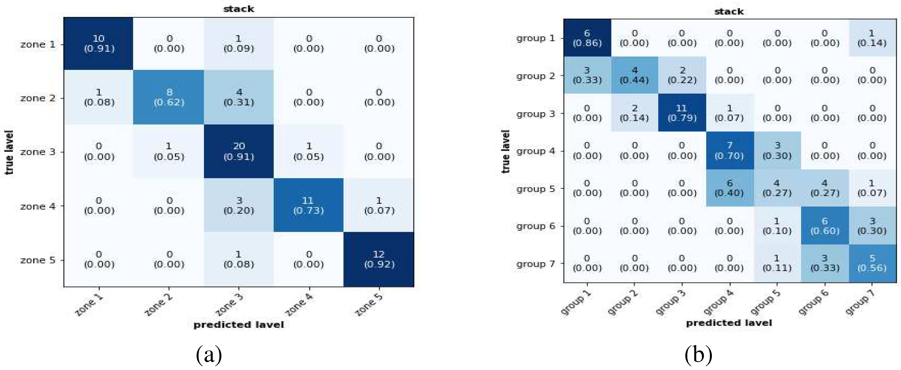
Figure 17 (a) and
17(b) show the confusion matrix for debonding location zone and size group predicted by the stacked model with test dataset. In the confusion matrix figure, the value in each square along the diagonal represents the number of true predicted labels and the value in the round-bracket shows the fraction of true class labels predicted accurately for particular class labels. The figure shows that prediction precision for a location zone varies from 0.92 to 0.62. For debonding size group prediction, the precision varied from 0.27 to 0.86. The overall performance of ML models in terms of AUC of DeepROC is listed in
Table 9. The values in the table help in reiterating the conclusion that the stacked model is better as compared to the base ML models in both debonding zone localization and size group prediction. It also shows again that location zone is better predicted than location size group. Overall, the ML models give a reasonable accuracy in both debonding location zone and size group predictions with FE transformed data.
5.4.6. Result with Experimental Data
After getting satisfactory results in debonding location zones and size group predictions with FE transformed data using ML model, the next task was to test the efficacy of the methodology with experimental data. Only the stacked model was considered for the experimental dataset. The two stacked models which were trained with FE transformed data for debonding location zone and size group dataset were tested with experimental dataset for location zone and size group prediction respectively. There were three damaged experimental specimens. Fifty experimental datasets were generated for each of them. They were used as input to the trained stacked models.
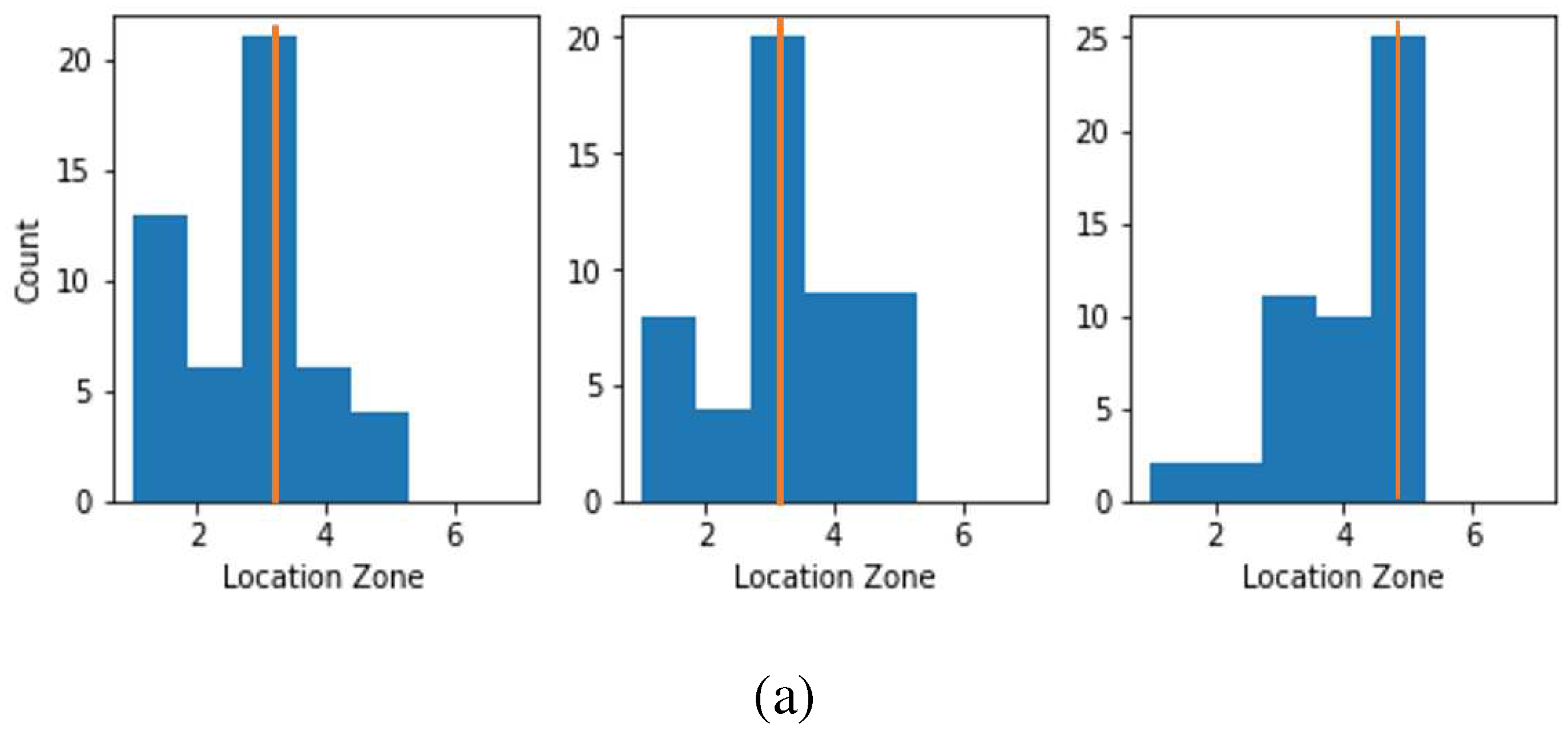
Figure 18(a) and
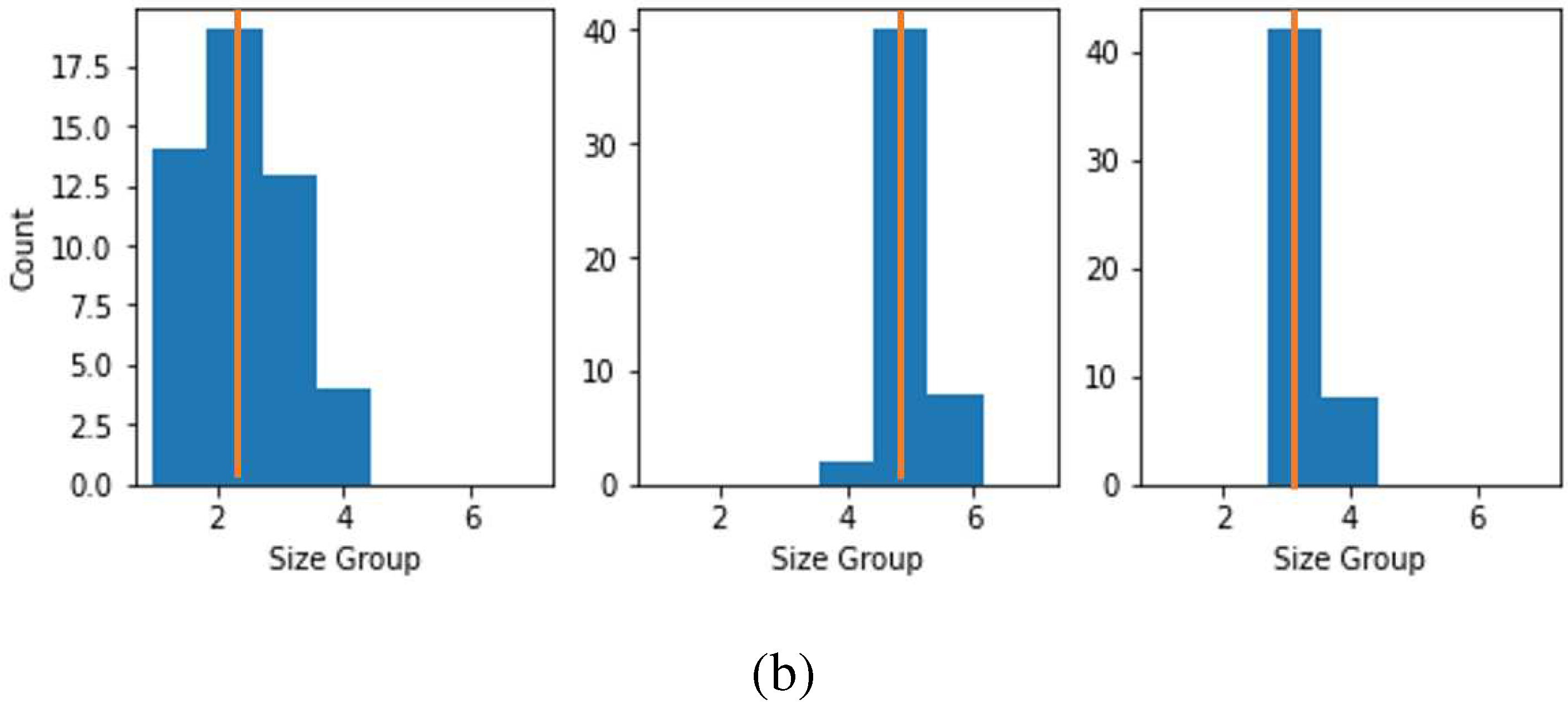
18 (b) show the prediction results for debonding location zone and size group respectively. The x-axes of the figures are the damage labels, the y-axes are the counts (i.e. the number of times a particular damage label has been predicted), and the yellow lines in the figure show the actual damage labels. From these figures, it can be seen that for the debonding zone location and size group, the predicted labels are populated around the actual class label. However, for debonding size groups, the maximum counts of predicted and actual labels are the same, which is not the case for location zone prediction. However, when stacked model trained with FE transformed data with 2 percent added gaussian noise the prediction accuracy with experimental data considerably improved for both debonding size group as well as debonding location zone as shown in
Figure 19.
6. Conclusions and Future Work
This work presents a new method of generating an FE database for SHM which is very close to an experimental database. The method used is a deep learning-based domain transfer model which transforms the FE domain data into experimental data and minimises the difference between them. The methodology is implemented for debonding localization and size estimation in metallic stiffened panels for vibration-based damage assessment. A bootstrapping technique was used to generate sufficient experimental data from a few samples of data collected from experiments using an LDV set-up. For FE simulated data, sufficient copies of data were created by adding noise to it. The FE simulated data was used as input and experimental data was used as target in the DL based DT model. This pretrained DT model (with undamaged experimental and FE simulated databases) was used to transform the FE simulated damaged database to the experimental domain. Three DT models were designed and their comparative study showed that a stacked DT model with a larger number of trainable parameters transformed the data into the experimental domain more effectively. This transformed FE dataset was used to train and evaluate ML models. Then, the trained ML model was tested with the experimentally obtained damage dataset. The results are satisfactory for predicting the debonding location zone and size group in stiffened panels.
The key contribution of this work is the establishment of a method of creation of a domain transfer model for generation of large databases from finite element based models which are very close to actual experimental results in their statistical distribution. Though this has been demonstrated with the specific example of debonding location and size prediction of stiffened panels using vibration signals, the technique has a much wider scope of application. It can be extended to other categories of structural health monitoring problems and even to other domains which share the difficulty of generating a large number of experimental data for training machine learning models.
Author Contributions
AK: conceptualization, data curation, formal analysis, investigation, methodology, software, validation, visualization, writing- original draft. AG: conceptualization, methodology, investigation, resources, supervision, writing- review and editing. SB: Experimental Resource, Investigation, Supervision.
Funding
This research received no external funding.
Institutional Review Board Statement
Not applicable.
Informed Consent Statement
Not applicable.
Data Availability Statement
The datasets generated during and/ or analysed during the current study are available from the corresponding author on reasonable request.
Acknowledgments
The author acknowledge the support provided by LDV lab, Aerospace department, IIT Bombay, during experiment work.
Conflicts of Interest
The authors declare no conflict of interest.
Appendix A
The architecture details of DT models
| Model-1 |
| Layer (type) |
Output Shape |
| Input |
(208) |
| Linear-1(Tanh) |
(1024) |
| Linear-2(Tanh) |
(512) |
| output |
(208) |
| Total parameters |
845520 |
| Model-2 |
| Layer (type) |
Output Shape |
| Input |
(208) |
| Conv1D-1(Tanh)(BN) |
(16, 103) |
| Conv1D-2(Tanh)(BN) |
(32, 50) |
| Conv1D-3(Tanh)(BN) |
(64, 24) |
| Conv1D-4(Tanh)(BN) |
(128, 11) |
| Linear-1(Tanh) |
(1024) |
| Linear-2(Tanh) |
(512) |
| output |
(208) |
| Total parameters |
2118112 |
| Model-3 |
| Layer (type) |
Output Shape |
| Input |
(208) |
| Conv1D-1(Tanh)(BN) |
(16, 103) |
| Conv1D-2(Tanh)(BN) |
(32, 50) |
| Conv1D-3(Tanh)(BN) |
(64, 24) |
| Conv1D-4(Tanh)(BN) |
(128, 11) |
| Linear-1(Tanh) |
(1024) |
| Linear-2(Tanh) |
(1408) |
| TransConv1D-1(Tanh)(BN) |
(64, 24) |
| TransConv1D-2(Tanh)(BN) |
(32, 50) |
| TransConv1D-3(Tanh) (BN) |
(16, 102) |
| Output |
(208) |
| Total parameters |
2905641 |
| BN = Batch Normalization, Conv1D = 1D-convolution channel. |
References
- C. R. Farrar, K. Worden, and J. Wiley, Structural Health Monitoring: A Machine learning Perspective. John Wiley and sons, 2012.
- E. Figueiredo, G. Park, C. R. Farrar, K. Worden, and J. Figueiras, “Machine learning algorithms for damage detection under operational and environmental variability,” Struct. Heal. Monit., vol. 10, no. 6, pp. 559–572, 2011. [CrossRef]
- Z. W. Z. Yang, H. Yang, T. Tian, D. Deng, M. Hu, J. Ma, D. Gao, J. Zhang, S. Ma, L. Yang, H. Xu, “A review in guided-ultrasonic-wave-based structural health monitoring: From fundamental theory to machine learning techniques,” Ultrasonics, vol. 133, p. 107014, 2023. [CrossRef]
- D. M. M. Gordan, S. R. Sabbagh-Yazdi, Z. Ismail, K. Ghaedi, P. Carroll and B. Samali, “State-of-the-art review on advancements of data mining in structural health monitoring,” Meas. J. Int. Meas. Confed., vol. 193, no. October 2021, 2022. [CrossRef]
- G. Toh and J. Park, “Review of Vibration-Based Structural Health Monitoring Using Deep Learning,” Appl. Sci., vol. 10, no. 5, 2020. [CrossRef]
- M. Azimi, A. D. Eslamlou, and G. Pekcan, “Data-Driven Structural Health Monitoring and Damage Detection through Deep Learning: State-of-the-Art Review,” Sensors, vol. 20, no. 10, 2020. [CrossRef]
- U. M. N. Jayawickrema, H. M. C. M. Herath, N. K. Hettiarachchi, H. P. Sooriyaarachchi, and J. A. Epaarachchi, “Fibre-optic sensor and deep learning-based structural health monitoring systems for civil structures: A review,” Meas. J. Int. Meas. Confed., vol. 199, no. May, p. 111543, 2022. [CrossRef]
- M. Civera and C. Surace, “Non-Destructive Techniques for the Condition and Structural Health Monitoring of Wind Turbines: A Literature Review of the Last 20 Years,” Sensors, vol. 22, no. 4, 2022. [CrossRef]
- C. Zhang, A. A. Mousavi, S. F. Masri, G. Gholipour, K. Yan, and X. Li, “Vibration feature extraction using signal processing techniques for structural health monitoring: A review,” Mech. Syst. Signal Process., vol. 177, p. 109175, 2022. [CrossRef]
- K. Eltouny, M. Gomaa, and X. Liang, “Unsupervised Learning Methods for Data-Driven Vibration-Based Structural Health Monitoring: A Review,” Sensors, vol. 23, no. 6, 2023. [CrossRef]
- J. N. Kudva, N. Munir, and P. W. Tan, “Damage detection in smart structures using neural networks and finite-element analyses,” Smart Mater. Struct., vol. 1, no. 2, pp. 108–112, 1992. [CrossRef]
- K. Worden, “Fault location in a framework structure using neural networks,” Smart Mater. Struct., vol. 3, 1993. [CrossRef]
- C. Sbarufatti, A. Manes, and M. Giglio, “Performance optimization of a diagnostic system based upon a simulated strain field for fatigue damage characterization,” Mech. Syst. Signal Process., vol. 40, no. 2, pp. 667–690, 2013. [CrossRef]
- C. Sbarufatti, G. Manson, and K. Worden, “A numerically-enhanced machine learning approach to damage diagnosis using a Lamb wave sensing network,” J. Sound Vib., vol. 333, no. 19, pp. 4499–4525, 2014. [CrossRef]
- Z. Su and L. Ye, “Lamb wave-based quantitative identification of delamination in CF/EP composite structures using artificial neural algorithm,” Compos. Struct., vol. 66, no. 1–4, pp. 627–637, 2004. [CrossRef]
- Z. su and L. ye, “Lamb Wave Propagation-based Damage Identification for Quasi-isotropic CF/EP Composite Laminates Using Artificial Neural Algorithm: Part I - Methodology and Database Development,” J. Intell. Mater. Syst. Struct., vol. 16, no. 2, pp. 97–111, 2005. [CrossRef]
- P. Gardner, X. Liu, and K. Worden, “On the application of domain adaptation in structural health monitoring,” Mech. Syst. Signal Process., vol. 138, p. 106550, 2020. [CrossRef]
- S. Zhang, C. M. Li, J. Yang, and W. Ye, “Effective combination of modeling and experimental data with deep metric learning for guided wave-based damage localization in plates,” Mech. Syst. Signal Process., vol. 172, no. March, p. 108979, 2022. [CrossRef]
- A. De Fenza, A. Sorrentino, and P. Vitiello, “Application of Artificial Neural Networks and Probability Ellipse methods for damage detection using Lamb waves,” Compos. Struct., vol. 133, pp. 390–403, 2015. [CrossRef]
- A. Kumar, A. Guha, and S. Banerjee, “A Methodology for Diagnosis of Damage by Machine Learning Algorithm on Experimental Data,” in Lecture Notes in Civil Engineering, 2021, vol. 128, pp. 91–105. [CrossRef]
- R. J. Barthorpe, G. Manson, and K. Worden, “On multi-site damage identification using single-site training data,” J. Sound Vib., vol. 409, pp. 43–64, 2017. [CrossRef]
- N. Bao, T. Zhang, R. Huang, S. Biswal, J. Su, and Y. Wang, “A Deep Transfer Learning Network for Structural Condition Identification with Limited Real-World Training Data,” Struct. Control Heal. Monit., vol. 2023, 2023. [CrossRef]
- C. Sbarufatti, A. Manes, and M. Giglio, “Performance optimization of a diagnostic system based upon a simulated strain field for fatigue damage characterization,” Mech. Syst. Signal Process., vol. 40, no. 2, pp. 667–690, 2013. [CrossRef]
- C. Sbarufatti, G. Manson, and K. Worden, “A numerically-enhanced machine learning approach to damage diagnosis using a Lamb wave sensing network,” J. Sound Vib., vol. 333, no. 19, pp. 4499–4525, 2014. [CrossRef]
- S. Zhang, C. M. Li, J. Yang, and W. Ye, “Effective combination of modeling and experimental data with deep metric learning for guided wave-based damage localization in plates,” Mech. Syst. Signal Process., vol. 172, Jun. 2022. [CrossRef]
- B. Efron and R. Tibshirani, “The Bootstrap Method for Assessing Statistical Accuracy,” Behaviormetrika, vol. 12, no. 17, pp. 1–35, 1985. [CrossRef]
- R. Semaan, “The uncertainty of the experimentally-measured momentum coefficient,” Exp. Fluids, vol. 61, no. 12, p. 248, 2020. [CrossRef]
- A. Carroll et al., “Improving Emotion Regulation, Well-being, and Neuro-cognitive Functioning in Teachers: a Matched Controlled Study Comparing the Mindfulness-Based Stress Reduction and Health Enhancement Programs,” Mindfulness (N. Y)., vol. 13, no. 1, pp. 123–144, 2022. [CrossRef]
- O. Mahmoud, F. Dudbridge, G. Davey Smith, M. Munafo, and K. Tilling, “A robust method for collider bias correction in conditional genome-wide association studies,” Nat. Commun., vol. 13, no. 1, p. 619, 2022. [CrossRef]
- L. Renault, J. C. McWilliams, and C. Kessouri, Faycal; Jousse, Alexandre; Frenzel, Hartmut; Chen, Ru; Deutsch, “Evaluation of high-resolution atmospheric and oceanic simulations of the California Current System,” Prog. Oceanogr., vol. 195, p. 102564, 2021. [CrossRef]
- T. Ince, S. Kiranyaz, L. Eren, M. Askar, and M. Gabbouj, “Real-Time Motor Fault Detection by 1-D Convolutional Neural Networks,” IEEE Trans. Ind. Electron., vol. 63, no. 11, pp. 7067–7075, 2016. [CrossRef]
- T. Zan, H. Wang, M. Wang, Z. Liu, and X. Gao, “Application of multi-dimension input convolutional neural network in fault diagnosis of rolling bearings,” Appl. Sci., vol. 9, no. 13, 2019. [CrossRef]
- O. Abdeljaber, O. Avci, S. Kiranyaz, M. Gabbouj, and D. J. Inman, “Real-time vibration-based structural damage detection using one-dimensional convolutional neural networks,” J. Sound Vib., vol. 388, pp. 154–170, 2017. [CrossRef]
- I. Goodfellow, Y. Bengio, and A. Courville, Deep Learning. MIT Press, 2016.
- S. Ioffe and C. Szegedy, “Batch normalization: Accelerating deep network training by reducing internal covariate shift,” 32nd Int. Conf. Mach. Learn. ICML 2015, vol. 1, pp. 448–456, 2015.
- C. M. Bishop, Neural Networks for Pattern Recognition. Oxford: Oxford University Press, 1995.
- K. Worden, G. Manson, and N. R. J. Fieller, “Damage detection using outlier analysis,” J. Sound Vib., vol. 229, no. 3, pp. 647–667, 2000. [CrossRef]
- C. Cortes and V. Vapnik, “Support-vector networks,” Mach. Learn., vol. 20, no. 3, pp. 273–297, 1995. [CrossRef]
- L. Breiman, “Random Forests,” Mach. Learn., vol. 45, no. 1, pp. 5–32, 2001. [CrossRef]
- T. Cover and P. Hart, “Nearest neighbor pattern classification,” IEEE Trans. Inf. Theory, vol. 13, no. 1, pp. 21–27, 1967. [CrossRef]
- D. H. Wolpert, “Stacked generalization,” Neural Networks, vol. 5, no. 2, pp. 241–259, 1992. [CrossRef]
- R. Aldave and J. P. Dussault, “Systematic Ensemble Learning for Regression,” pp. 1–38, 2014, [Online]. Available: http://arxiv.org/abs/1403.7267.
- C. Cao and Z. Wang, “IMCStacking: Cost-sensitive stacking learning with feature inverse mapping for imbalanced problems,” Knowledge-Based Syst., vol. 150, pp. 27–37, 2018. [CrossRef]
- A. Kumar, A. Guha, and S. Banerjee, “Improving Prediction Accuracy for Debonding Quantification in Stiffened Plate by Meta-Learning Model,” in Proceedings of International Conference on Big Data, Machine Learning and their Applications, 2021, pp. 51–63. [CrossRef]
- B. Zhai and J. Chen, “Development of a stacked ensemble model for forecasting and analyzing daily average PM2.5 concentrations in Beijing, China,” Sci. Total Environ., vol. 635, pp. 644–658, 2018. [CrossRef]
- M. Ozay and F. T. Yarman-Vural, “Hierarchical distance learning by stacking nearest neighbor classifiers,” Inf. Fusion, vol. 29, pp. 14–31, 2016. [CrossRef]
- A. M. Carrington et al., “Deep ROC Analysis and AUC as Balanced Average Accuracy, for Improved Classifier Selection, Audit and Explanation,” IEEE Trans. Pattern Anal. Mach. Intell., vol. 45, no. 1, pp. 329–341, 2023. [CrossRef]
- A. M. Carrington et al., “A new concordant partial AUC and partial c statistic for imbalanced data in the evaluation of machine learning algorithms,” BMC Med. Inform. Decis. Mak., vol. 20, no. 1, pp. 1–12, 2020. [CrossRef]
Figure 1.
Schematic representation of domain transfer.
Figure 1.
Schematic representation of domain transfer.
Figure 2.
Domain transfer-based SHM methodology framework.
Figure 2.
Domain transfer-based SHM methodology framework.
Figure 3.
Bootstrap sampling procedure and sampling distribution estimation using Q-Q plot.
Figure 3.
Bootstrap sampling procedure and sampling distribution estimation using Q-Q plot.
Figure 4.
Schematic domain transfer model.
Figure 4.
Schematic domain transfer model.
Figure 5.
Sequence of order of transformed dataset to damage assessment.
Figure 5.
Sequence of order of transformed dataset to damage assessment.
Figure 6.
Experimental set up of LDV.
Figure 6.
Experimental set up of LDV.
Figure 7.
(a) Specimen top view (b) cross-section of stiffened panel (c) white painted back side of specimen (d) defined scan points (e) 1st mode shape.
Figure 7.
(a) Specimen top view (b) cross-section of stiffened panel (c) white painted back side of specimen (d) defined scan points (e) 1st mode shape.
Figure 8.
Symmetry of stiffened panel.
Figure 8.
Symmetry of stiffened panel.
Figure 9.
(a) Initial 35 number collected data (b) 200 bootstrapped sample data (c) Q-Q plot for normal distribution.
Figure 9.
(a) Initial 35 number collected data (b) 200 bootstrapped sample data (c) Q-Q plot for normal distribution.
Figure 10.
Tanh Activation function.
Figure 10.
Tanh Activation function.
Figure 11.
Types of domain transformation model, Model-1 as Deep Neural Network, Model-2 as 1D-CNN and Model-3 as 1D-CNN-FC-CNN.
Figure 11.
Types of domain transformation model, Model-1 as Deep Neural Network, Model-2 as 1D-CNN and Model-3 as 1D-CNN-FC-CNN.
Figure 12.
Training processes of the DT models in terms of epoch vs. log loss for (a) model-1 (b) model-2 (c) model-3.
Figure 12.
Training processes of the DT models in terms of epoch vs. log loss for (a) model-1 (b) model-2 (c) model-3.
Figure 13.
(a) Average construction RMSE (b) ML model debonding localization performance on FE transformed dataset using DT models 1,2 and 3.
Figure 13.
(a) Average construction RMSE (b) ML model debonding localization performance on FE transformed dataset using DT models 1,2 and 3.
Figure 14.
The first vibrational mode shape displacement data for scan point 1 to 208 (one-symmetric part) (a) Original FE simulated and experimental (b) transformed FE simulated and experimental data for debonding of 50 mm at 265 mm.
Figure 14.
The first vibrational mode shape displacement data for scan point 1 to 208 (one-symmetric part) (a) Original FE simulated and experimental (b) transformed FE simulated and experimental data for debonding of 50 mm at 265 mm.
Figure 15.
Estimated MSD value for debonding size 10 mm to 150 mm located at 265 mm.
Figure 15.
Estimated MSD value for debonding size 10 mm to 150 mm located at 265 mm.
Figure 16.
(a) Threshold MSD value (b) the filtered feature vector (blue-dot).
Figure 16.
(a) Threshold MSD value (b) the filtered feature vector (blue-dot).
Figure 17.
Confusion matrix for (a) Debonding location zone and (b) debonding size group predicted by stacked model.
Figure 17.
Confusion matrix for (a) Debonding location zone and (b) debonding size group predicted by stacked model.
Figure 18.
Result with experimental data, when stacked model trained with FE transformed data without noise for debonding (a) location zone (b) size group, the histogram shows predicted label and actual labels is in yellow line.
Figure 18.
Result with experimental data, when stacked model trained with FE transformed data without noise for debonding (a) location zone (b) size group, the histogram shows predicted label and actual labels is in yellow line.
Figure 19.
Result with experimental data, when stacked model trained with FE transformed data with 2 percent gaussian noise for debonding (a) location zone (b) size group, the histogram shows predicted label and actual labels is in yellow line.
Figure 19.
Result with experimental data, when stacked model trained with FE transformed data with 2 percent gaussian noise for debonding (a) location zone (b) size group, the histogram shows predicted label and actual labels is in yellow line.
Table 1.
Related work for lack of availability of damage data in SHM.
Table 1.
Related work for lack of availability of damage data in SHM.
| Authors |
Method |
Approach |
Structure |
Damage type |
Exp. data quantity |
| Sbarufatti et al., 2013[23] |
Scaling factor |
Strain field |
Helicopter fuselage |
Fatigue damage |
Less Exp. data |
| Sbarufatti et al., 2013[24] |
Numerically-enhanced ML approach |
Guided Wave |
Plate |
Discontinuity |
Less Exp. data |
| Barthorpe and Worden 2017[21] |
Generating exp. data from one specimen |
Vibration |
Wing panel of aero plane |
Discontinuity |
High Exp. data |
| Gardner and Worden 2019[17] |
Domain adaptation |
Vibration |
MDOF spring mass system |
Stiffness variation |
Less Exp. data |
| Zhang et al., 2022[25] |
Effective combination FE and exp. data |
Guided wave |
Plate |
Discontinuity |
Equal quantity of FE and exp. data |
| Bao et al., 2023[22] |
Transfer Learning |
Vibration |
Portal frame |
Nut-bolt loosening |
Relatively more exp. data |
Table 2.
Test Specimens.
| Specimen 1 |
Specimen 2 |
Specimen 3 |
Specimen 4 |
| Intact (Undamaged) |
Debonding at
X=265 of L = 50 |
Debonding at
X=265 of L = 100 |
Debonding at
X=285 of L = 70 |
Table 3.
Experimental parameters.
Table 3.
Experimental parameters.
| Parameters |
Value |
| Minimum speed |
5 µm /s |
| Maximum speed |
10 m/s |
| Frequency Resolution |
0.125 Hz |
| Frequency Range |
0-200 Hz |
| Number of FFT lines |
12800 |
| Scan time for one scan point |
64 sec. |
Table 4.
Contact modelling parameters.
Table 4.
Contact modelling parameters.
| Parameter |
Type |
| Contact type |
Flexible surface-to-surface |
| Target element |
TARGE170 |
| Contact element |
CONTA174 |
| Contact algorithm |
Augmented Lagrange Method |
| Location of contact detection |
Gauss point |
| Contact selection |
Asymmetric |
| Gap/closure |
No adjustment |
| Behavior of the contact surface |
No Separation |
| Geometry |
3-D |
Table 5.
Model frequency (Hz).
Table 5.
Model frequency (Hz).
| |
Undamaged |
50 mm debonding |
100 mm debonding |
| Mode |
1 |
2 |
3 |
1 |
2 |
3 |
1 |
2 |
3 |
| FEM |
49.953 |
70.009 |
110.26 |
49.918 |
69.738 |
109.43 |
49.913 |
69.342 |
109.43 |
| Experiment |
49.37 |
68.22 |
105.9 |
49.296 |
68.12 |
105.51 |
49.12 |
67.86 |
104.95 |
Table 6.
Debonding Zone division.
Table 6.
Debonding Zone division.
Debonding
Location(X) |
105,125,
145 |
165,185,205 |
225,245,265,285,
305 |
325,345,365 |
385,405,425 |
| Debonding Zone |
Zone-1 |
Zone-2 |
Zone-3 |
Zone-4 |
Zone-5 |
Table 7.
Debonding location zones.
Table 7.
Debonding location zones.
Debonding
Location(X) |
105,125,145 |
165,185,205 |
225,245,265,285,
305 |
325,345,365 |
385,405,425 |
| Debonding Zone |
Zone-1 |
Zone-2 |
Zone-3 |
Zone-4 |
Zone-5 |
Table 8.
Debonding size groups.
Table 8.
Debonding size groups.
| Debonding Size (mm) |
10,15,20,
25,30 |
35,40,
45,50,55 |
60,65,70,
75 |
80,85,90,
95 |
100,105,
110,115 |
120,125,
130,135 |
140,145,
150 |
| Size Group |
Group-1 |
Group-2 |
Group-3 |
Group-4 |
Group-5 |
Group-6 |
Group-7 |
Table 9.
AUC for DeepROC for ML models.
Table 9.
AUC for DeepROC for ML models.
| ML Model |
Location
AUC (DeepROC) |
Size
AUC (DeepROC) |
| SVM |
0.717 |
0.720 |
| RF |
0.785 |
0.905 |
| ABC |
0.549 |
0.6823 |
| GBC |
0.588 |
0.907 |
| k-nn |
0.632 |
0.887 |
| Stack |
0.920 |
0.952 |
|
Disclaimer/Publisher’s Note: The statements, opinions and data contained in all publications are solely those of the individual author(s) and contributor(s) and not of MDPI and/or the editor(s). MDPI and/or the editor(s) disclaim responsibility for any injury to people or property resulting from any ideas, methods, instructions or products referred to in the content. |
© 2023 by the authors. Licensee MDPI, Basel, Switzerland. This article is an open access article distributed under the terms and conditions of the Creative Commons Attribution (CC BY) license (http://creativecommons.org/licenses/by/4.0/).
