Preprint

Article

A Machine Learning Algorithm That Experiences Evolutionary Algorithm’s Predictions – Application to Optimal Control.

Altmetrics

Downloads

Views

Comments

A peer-reviewed article of this preprint also exists.

This version is not peer-reviewed

Submitted:

11 December 2023

Posted:

12 December 2023

You are already at the latest version

Alerts

Abstract

Using metaheuristics, such as the Evolutionary Algorithm (EA), within control structures is a realistic approach for certain optimal control problems. Their role is often predicting the optimal control values over a prediction horizon using a process model (PM). The big computational effort sometimes causes problems. Our work addresses a new issue: whether a machine learning (ML) algorithm could “learn” the optimal behaviour of the couple (EA, PM). A positive answer is given by proposing datasets apprehending this couple's optimal behaviour and appropriate ML models. Following a design procedure, a number of closed-loop simulations will provide the sequences of optimal control and state values, which are collected and aggregated in a data structure. For each sampling period, datasets are extracted from the aggregated data. The ML algorithm experiencing these datasets will produce a set of regression functions. Replacing the EA predictor with the ML model, new simulations are carried out, proving that the state evolution is almost identical. The execution time decreases drastically because the PM’s numerical integrations are totally avoided. The performance index equals the best-known value. In different case studies, the ML models succeeded in capturing the optimal behaviour of the couple (EA, PM) and yielded efficient controllers.

Keywords:

Subject: Computer Science and Mathematics - Artificial Intelligence and Machine Learning

1. Introduction

Controlling a process subjected to a performance index is a usual task in process engineering. Theoretical control laws can be implemented in favourable situations where the process has certain mathematical properties. On the other hand, when the process has profound nonlinearities, or its model is uncertain, imprecise or incomplete, using metaheuristic algorithms (EA, Particle Swarm Optimization, etc.) (see [1,2,3]) within an appropriate control structure could be a realistic solution. Control engineering recorded many examples of using metaheuristics [4,5,6,7,8,9] owing to their robustness and capacity to cope with complex problems.

Generally speaking, the metaheuristic algorithm’s role within a controller is to predict the optimal (quasi-optimal) control values. The predictor forecasts the optimal control sequence for a prediction horizon, and the controller decides the next optimal control value. A control structure adequate for this kind of controller is Receding Horizon Control (RHC) [10,11,12,13]. It can be used to solve Optimal Control Problems (OCPs) and includes a Process Model (PM) [14,15,16].

The authors have studied implementing the prediction module using EAs in previous works [16,17,18]. EAs proved a realistic solution due to many possibilities to reduce the predictor’s execution time. The latter is the big challenge of this approach, mainly appropriate for slow processes with large sampling periods because of the predictions’ computation time. Extending their applicability is a challenge, involving techniques and control structures diminishing the execution time [19,20,21]. One can consider that our work addresses the execution time’s decreasing, but the proposed machine learning (ML) task (see [22,23,24,25]) largely exceeds this topic.

This work proposes an interesting issue: whether a machine learning algorithm could “learn” the optimal behaviour of the couple (EA, PM). A positive answer would have very favourable consequences for the controller implementation. The substitution of the couple (EA, PM) with an accurate ML algorithm could cause the predictions’ computation time to decrease significantly and the controller’s structure to be much simpler. In this context, the ML algorithm has to construct usable models experiencing datasets catching the optimal behaviour of the couple (EA, PM). Concretely, this work’s main objective is to answer the above-mentioned question positively by proposing

realistic datasets apprehending the optimal behaviour of the couple (EA, PM) and
appropriate ML models.

Hence, this work will propose an ML model that can substitute the couple (EA, PM) inside the optimal controller while keeping the control performances. In other words, the ML model would be equivalent in a certain sense to the optimal behaviour of the EA plus PM; both entities are predictors [26]. According to our knowledge, this “intelligent equivalence” can be considered a new issue.

Before using the controller within the closed-loop system in real-time, a simulation program must validate the designed controller through the Process’s evolution along the imposed control horizon; the Process and the PM are considered identical. The simulation’s results are usually sequences of control and state variables’ values along the control horizon that can be stored or recorded. This data is a mark of the system’s evolution made up of the control profile (sequence of control values) and state trajectory (sequence of state variables’ values). Repeating the simulation many times, we can aggregate these data and generate datasets for the ML algorithm. The simulations are conducted offline, so there is no execution time constraint.

An important remark is that we do not need data from the real Process to be included in the datasets. The predictor module predicts optimal trajectories using only the EA and PM, whose inter-influence must be captured by the datasets. When an accurate ML model replaces the initial predictor, the controller should behave quasi-identically within simulations, which is our desideratum.

This work will ascertain the previous considerations and propose an approach to construct the datasets and ML model, starting from the OCP to solve. Besides general considerations, we will apply the proposed methods to a specific OCP, exemplifying the proposed methods and algorithms to make the presentation easy to follow.

We shall consider OCPs with a final cost that uses predictions to exemplify the equivalence mentioned above and implement ML controllers. Section 2 recalls the general approach to solving the OCPs using EAs developed in previous authors’ works [16,19,20,21]. The Park Ramirez Problem (PRP) (see [21,27,28]) is a kind of benchmark problem already treated in this context, which is addressed as an example. This paper will report partially previous results for comparison and take over the EA predictor’s implementation. Section 2 is mainly necessary because the optimal control using the EA will supply the datasets for ML. Although the aspects presented in this section are not among this paper’s contributions, they introduce the notations and keep the discourse self-contained.

Section 3 answers the following three basic questions:

What data do we need to capture the optimal behaviour of the couple (EA, PM)?
How do we generate the datasets for the ML algorithm?
What ML model can be used to design an appropriate controller (we will name it ML controller)?

These a general questions, each of which has subsumed aspects to clarify. Section 3.1, describing the proposed method, answers these questions succinctly; details will be given in the next sections. It also establishes a controller design procedure.

The starting point in our approach is that we have already solved the considered OCP, and the implemented controller has a prediction module using a specific EA. Section 3.2.1 describes an algorithm achieving the closed-loop simulation along the control horizon devoted to the EA predictor. The simulation will record the sequence of optimal control values - the optimal control profile - and the optimal trajectory (sequence of states). The two sequences can be regarded as a series of couples (state, control value), each couple associated implicitly with a sampling period.

Repeating the simulation M times (e.g. M equals 200), data concerning these optimal evolutions of the closed loop is collected and aggregated into a data structure presented in section 3.2.2. These aggregated data structure characterizes the optimal behaviour of the couple (EA, PM) globally, that is, for the whole control horizon. The extraction of datasets characterizing each sampling period from the aggregated data creates the premise to find a model of optimal behaviour for each sampling period. Section 3.2.3 describes how the aggregated data is split into datasets for each sampling period. Moreover, training and testing datasets are created.

In section 3.3, the ML models are constructed according to an important choice. The ML model will be a set of regression functions; a linear regression function will be determined for each sampling period [29,30,31]. The first reason for this choice is the model’s simplicity, which is important, especially when the control horizon is large. Secondly, the control law will be directly determined. This fact is appropriate for the controller implementation, which is now straightforward. Section 3.3.1 proposes simple models with linear terms for each state variable. In contrast, section 3.3.2 uses the stepwise regression strategy to generate regression functions, which are allowed to include nonlinear terms as the interactions. The ML model succeeds in reproducing the optimal behaviour of the EA predictor with a high accuracy.

The simulation of the closed-loop system is the way to test the generalization aptitude of the new predictor after its implementation. In its first part, Section 4 describes an algorithm that simulates the closed-loop system using the ML controller along the control horizon. The second part compares the simulation results to those anteriorly obtained with the EA predictor for the PRP case [21]. The state evolutions are practically identical, and the performance index equals the best of M evolutions, which is true for the two types of regression functions.

The simulation results (in the PRP case and other case studies not presented in this paper) proved that the proposed ML models succeeded in apprehending the optimal behaviour of the couple (EA, PM) and engendered efficient controllers.

We consider that our work has the following findings:

the interesting issue itself, which is to find an ML model experiencing the datasets generated by an EA (or another metaheuristic), trying to capture the latter’s optimal behaviour.
the dataset’s construction as a dynamic trace of the EA predictor, aggregating the trajectories and CPs.
the dataset extraction for each sampling period as a premise to find a temporally distributed ML model.
the design procedure for the ML controller and all associated algorithms (simulation and models’ construction algorithms).
the outstanding decrease in the ML controller’s execution time.

Special attention was addressed to the implementation aspects such that the interested reader can find support to apprehend and eventually reproduce parts of this work or use it in other projects. With this aim in view, all algorithms used in this work are implemented, the associated scripts are attached as supplementary materials, and all the necessary details are given in the Appendixes.

2. Optimal control using Evolutionary Algorithms.

This section recalls the general approach to solving the OCPs using EAs developed in anterior papers [19,21]. The minimal elements presented here introduce the notations and keep the discourse self-contained.

2.1. Optimal control problems with a final cost

The structure of an OCP being well-known, we consider in the sequel only the defining elements adapted to the problem taken as an example in this section. Rigorous mathematical details will be avoided to simplify the presentation.

2.1.1. Process Model

In our approach, the controller includes a process model constituted by algebraic and ordinary differential equations: Preprints 92978 i001

An example of a Process Model is equation (7) from subsection 2.1.4

2.1.2. Constraints

There are many constraint types, but we mention only those used in the case study presented in this paper. Preprints 92978 i002

The values

u_{\min}^{j}, u_{\max}^{j}

are the technological bounds of the variable

u_{j} (t)

If T is the sampling period of the control system, we can divide the control horizon into H sampling periods:

t_{f i n a l} = H \times T .

2.1.3. Cost function

The problem is to determine the control function

U (\cdot)

optimizing (max or min) a specific cost (objective) function J, whose general form is given below:

J (U (\cdot), X_{0}) = \int_{0}^{t_{f i n a l}} L (X (τ), U (τ)) d τ + J_{f i n a l}

(5)

The function L determines the integral component (Lagrange term) of function J, while J_final (Mayer term) rewards (or penalizes) the final state (in most cases).

Remark 1.

When the final cost is present, and the controller makes predictions, whether or not there is an integral term, the prediction horizon must end at the final time, involving the biggest computational complexity.

Given remark 1, we consider only the final cost, a situation suited to our OCP (see next section).

J (U (\cdot), X_{0}) ≜ J_{f i n a l} = J (X (t_{f i n a l}))

The problem’s solution is the function U(·) that engenders the cost function’s optimal value. This value, J₀, is called the performance index:

J_{0} = \underset{U (\cdot)}{m a x} J (X (t_{f i n a l})) ≜ \underset{U (\cdot)}{m a x} J (U (\cdot), X_{0})

(6)

2.1.4. An example of OCP with a final cost

Park–Ramirez problem (PRP) is a kind of benchmark problem ([21,27,28]) that can exemplify a final cost OCP. The nonlinear process models a fed-batch reactor, which produces secreted protein. This problem has been addressed in many works to study integration methods.

Process Model (PM) Preprints 92978 i003

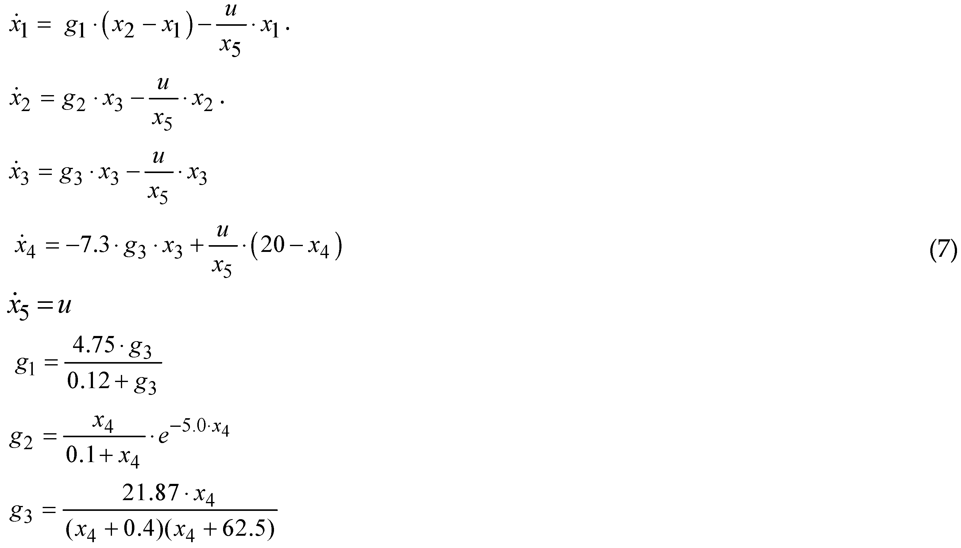
The state vector

X (t) = {[x_{1} (t) \dots x_{5} (t)]}^{T}

regroups the following physical parameters:

x_{1} (t)

- concentration of secreted protein,

x_{2} (t)

- concentration of total protein,

x_{3} (t)

- density of culture cell,

x_{4} (t)

- concentration of substrate,

x_{5} (t)

-holdup volume.

It holds: n=5; m=1;

U (t) = u (t) \in R

Constraints Preprints 92978 i004

Performance Index

J_{0} = \max_{u (t)} J (x (t_{f i n a l})) = \max_{u (t)} X_{1} (t_{f i n a l}) \cdot X_{5} (t_{f i n a l})

An open-loop solution can not be used in real-time because the Process and PM have different dynamics (even when there are small differences); this will produce unpredictable efficiency. We want to generate a controlled optimal process (a closed-loop solution) starting from a given X₀ whose final cost should be J₀.

2.2. A discrete-time solution based on EAs

A control structure that can generate the optimal solution is RHC ([16,21]). Its controller includes the process model and a prediction module (see Figure 1). The last one predicts, at each moment kT, the optimal control sequence until the final time. Then, the controller outputs this sequence’s first element as the optimal value and inputs the next Process’s state.

The prediction module using an EA proved a realistic solution due to many possibilities to reduce its execution time [19,20,21].

To use an EA, we append to our OCP the discretization constraint:

U (t) = U (k T), for k \cdot T \leq t < (k + 1) \cdot T; k = 0, \dots, H - 1 .

So, the control variables are step functions. For the sake of simplicity, the time moment

k \cdot T

will be denoted in the sequel. For example, inside the sampling period

[k T, (k + 1) T)

, the control vector is

U (k T) \equiv U (k) ≜ {[u_{1} (k), \dots, u_{m} (k)]}^{T}

We name a “control profile” (CP) a complete sequence of H control vectors,

U (0), U (1), \dots U (H - 1)

. It will generate the transfer diagram drawn in Figure 2.

The EA yields candidate predictions over prediction horizons and evaluates the cost function J. For the sampling period [k, k+1), a candidate prediction is a control sequence having the following structure:

\bar{U} (k) = 〈U (k), \dots, U (H - 1)〉 .

(8)

The vector

X (k)

is the process’s current state. It is also the initial state for the candidate prediction with H-k elements. This fact justifies the appellation of “Receding Horizon Control”. Using equations (1) and (8), the EA also calculates the corresponding state sequence (with H-k+1 elements):

\bar{X} (k) = 〈X (k), \dots, X (H)〉

(9)

At convergence, the EA returns (to the controller) the optimal prediction sequence, denoted

\bar{V} (k)

\bar{V} (k) ≜ \arg \max_{\bar{U} (k)} J (\bar{U} (k), X (k)) = 〈V (k), \dots, V (H - 1)〉

(10)

Finally, the first value of the sequence, V(k), becomes the controller’s best output, denoted U^*(k), sent toward the process:

U^{*} (k) ≜ V (k)

(11)

Remark 2.

The optimal control

U^{*} (k)

is also a function of the current state

X (k)

, which does not appear as a distinct argument in (11) to keep the notation simple and easy to follow. Nevertheless, this dependence is essential for the machine learning models as well.

The other values of the sequence

\bar{V} (k)

are forgotten, and the controller will treat the next sampling period [k+1, k+2).

The controller equipped with the EA constructs the optimal CP for the given initial state X₀=X(0) and the entire control horizon, concatenating the optimal controls

U^{*} (k)

k = 0, \dots, H - 1

. It forces the system to pass through a sequence of “optimal states”, the optimal trajectory

Γ (X_{0})

Ω (X_{0}) ≜ 〈U^{*} (0), U^{*} (1), \dots, U^{*} (H - 1)〉

(12)

Γ (X_{0}) ≜ 〈X_{0}, X^{*} (1), \dots, X^{*} (H)〉

(13)

These two sequences completely characterize the optimal evolution of the closed loop over the control horizon. Theoretically, the optimal cost function will reach the value J₀ if the process and its model are identical. Practically, this value will be very close to J₀, such that Ω(X₀) is a quasi-optimal solution of our OCP.

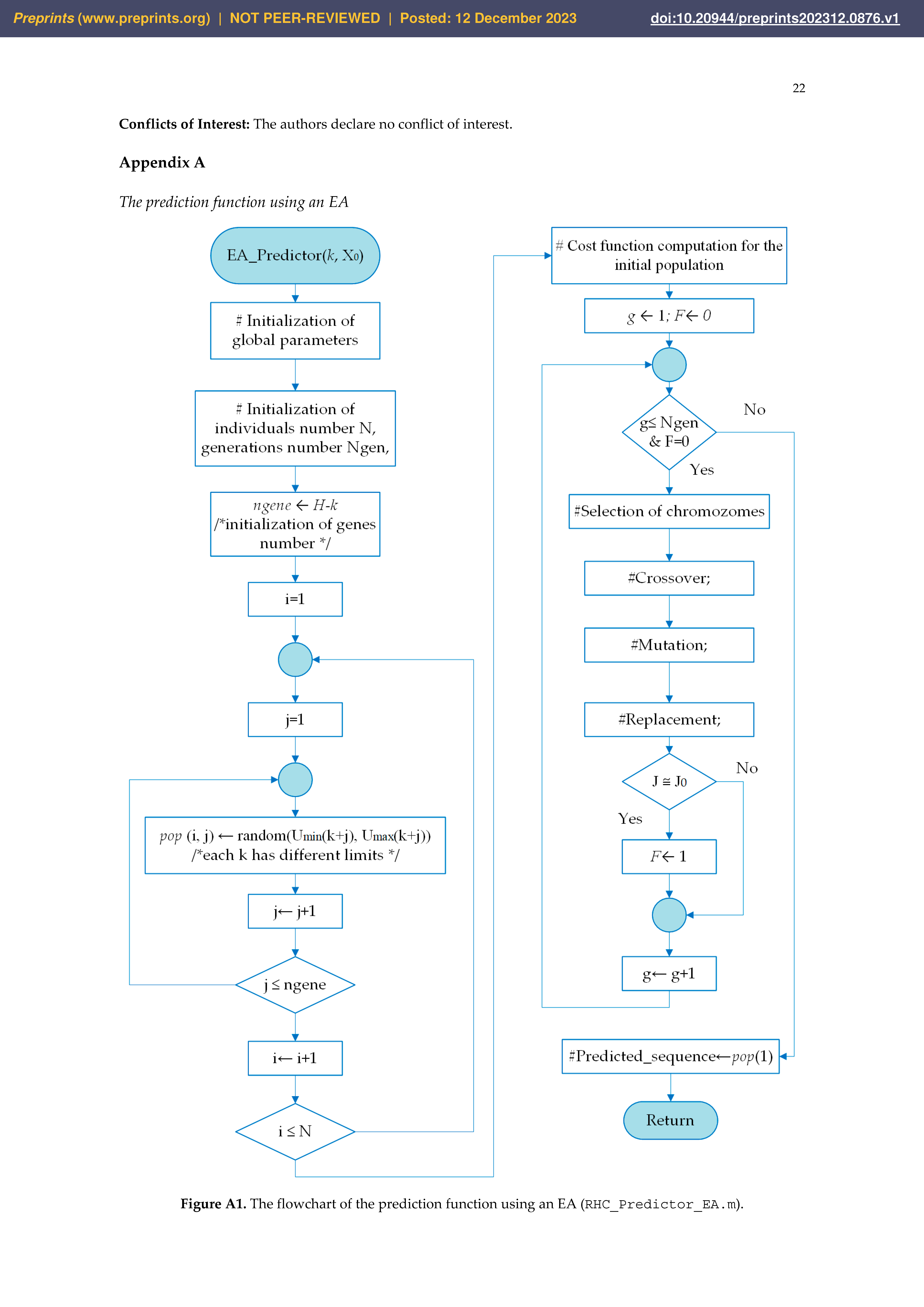
The flowchart of the prediction module is drawn in Appendix A. The interested reader can find the main characteristics of the implemented EA in [21] or the supplementary materials appended to this work. In our implementation, the EA’s code is presented in the script RHC_Predictor_EA.m. The initial population is generated using the control variables’ bounds. The cost function is coded within the file eval_PR_step.m. All scripts are included in the folder ART_Math, as the other functions called by the predictor and implementing the EA’s operators and the PM.

3. Controller based on machine learning

3.1. The general description of the proposed method

The PRP and other problems of this kind allow the validation of the designed optimal controller by simulating the control loop.

Simulation of the control loop is an important design tool in this context, which can supply the sequence

Ω (X_{0})

and

Γ (X_{0})

( (12) and (13)) that describe the quasi-optimal evolution of the loop.

Repeating the control loop simulation M times, we obtain M different optimal (actually quasi-optimal) couples (CP – trajectory), even if the initial states would be identical due to the EA’s stochastic character. Moreover, in the case of PRP, the initial state can be perturbed to simulate the imperfect realization of the initial conditions when launching a new batch. Let us consider a lot of the M simulations illustrated in Figure 3.

At step k of the control horizon, the controller must predict the optimal control output (sent toward the process) using its predictor module based on the EA and MP described before. Data concerning the same step have some common aspects:

The initial process’s state $X_{i}^{*} (k), 1 \leq i \leq M$ is input data for the EA.
The prediction horizon is the same: H – k.
The PM is the same.
The M simulations use the same EA.

The EA calculates and returns the optimal control vector

U_{i}^{*} (k), 1 \leq i \leq M

. A dataset including the simulation results for step k can be constructed as follows:

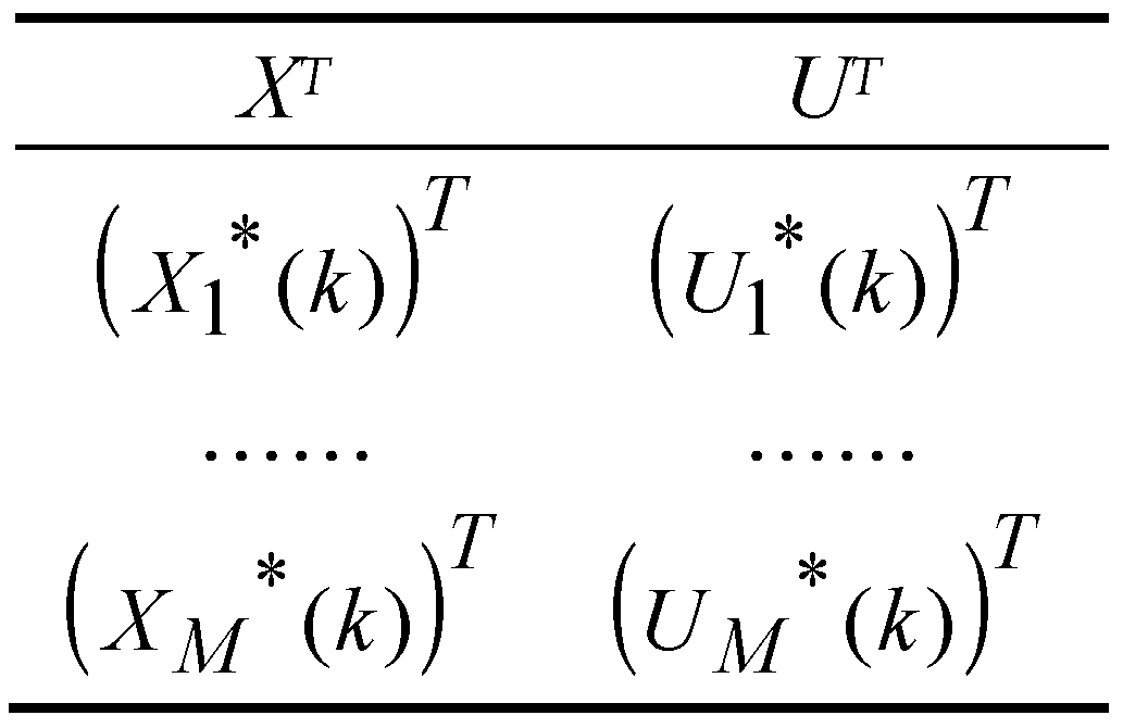
The dataset gets the look of a table due to the transposition operator. If M is big enough, this dataset collects an essential part of the EA’s ability to predict optimal control values for step k. It would be useful to answer the question: How can we generalize this ability for other current state values the process could access at step k? A machine learning algorithm is the answer. For example, linear regression (see [29,31]) can construct a function

f_{k} : R^{n} \to R^{m}

for each

k, k = 0, 1, \dots, H - 1

using a dataset like that presented before.

Remark 3.

The linear regression function

f_{k}

models how the EA determines the optimal prediction at step k. The set of functions

Φ = {f_{k} |k = 0, 1, \dots, H - 1}

is the couple (EA–PM) machine-learning model. The behaviour of the EA, which, in turn, depends on the PM, is captured by the set of functions

Φ

Hence, it would be possible to successfully replace the predictor with EA by this set of functions and obtain a faster controller.

Logically, a few steps lead us to a design procedure for the optimal controller.

Design procedure

Implement a program to simulate the closed loop functioning over the control horizon (H) using the controller based on the EA. To simplify the presentation, we will call it in the sequel ControlLoop_EA. The output data are the quasi-optimal trajectory and its associated control profile ( $Ω (X_{0})$ and $Γ (X_{0})$ ).
Repeat M times the module ControlLoop_EA to generate and save M quasi-optimal trajectories and their control profiles.
Extract, for each step k, datasets similar to Table 1 using the data saved at step 2.
Determine the machine-learning model (for example, the set of functions $Φ$ ) experiencing the M trajectories and control profiles.
Implement the new controller based on ML. It will be called ML_controller in the sequel.

Simulation of the closed loop using the new controller
Write a simulation program called ControlLoop_ML for the closed loop working with the new controller. This simulation will test the feasibility of the proposed method, the quality of the quasi-optimal solution, the performance index, and the execution time of the new controller.

The set of functions

Φ

can determine the optimal CP starting from a given state

X_{0}

, following the transfer diagram from Figure 2, and applying the functions

f_{0}, f_{1}, \dots, f_{H - 1}

to the current state successively:

U_{1}^{*} = f_{0} (X_{0}); U_{2}^{*} = f_{1} (X_{1}); \dots U_{H - 1}^{*} = (X_{H - 1}) .

(14)

Remark 4.

The design procedure shows that the new controller is completely designed offline. No data collected online from the process is necessary. The result of this procedure is the new Controller, ML_controller, which could be used in real-time after a robustness analysis.

3.2. Dataset generation for machine learning model

The first two steps of the design procedure will be described in this section, trying to keep generality. Only some aspects will refer to the PRP to simplify the presentation.

3.2.1. The simulation of the closed-loop system based on EA predictions

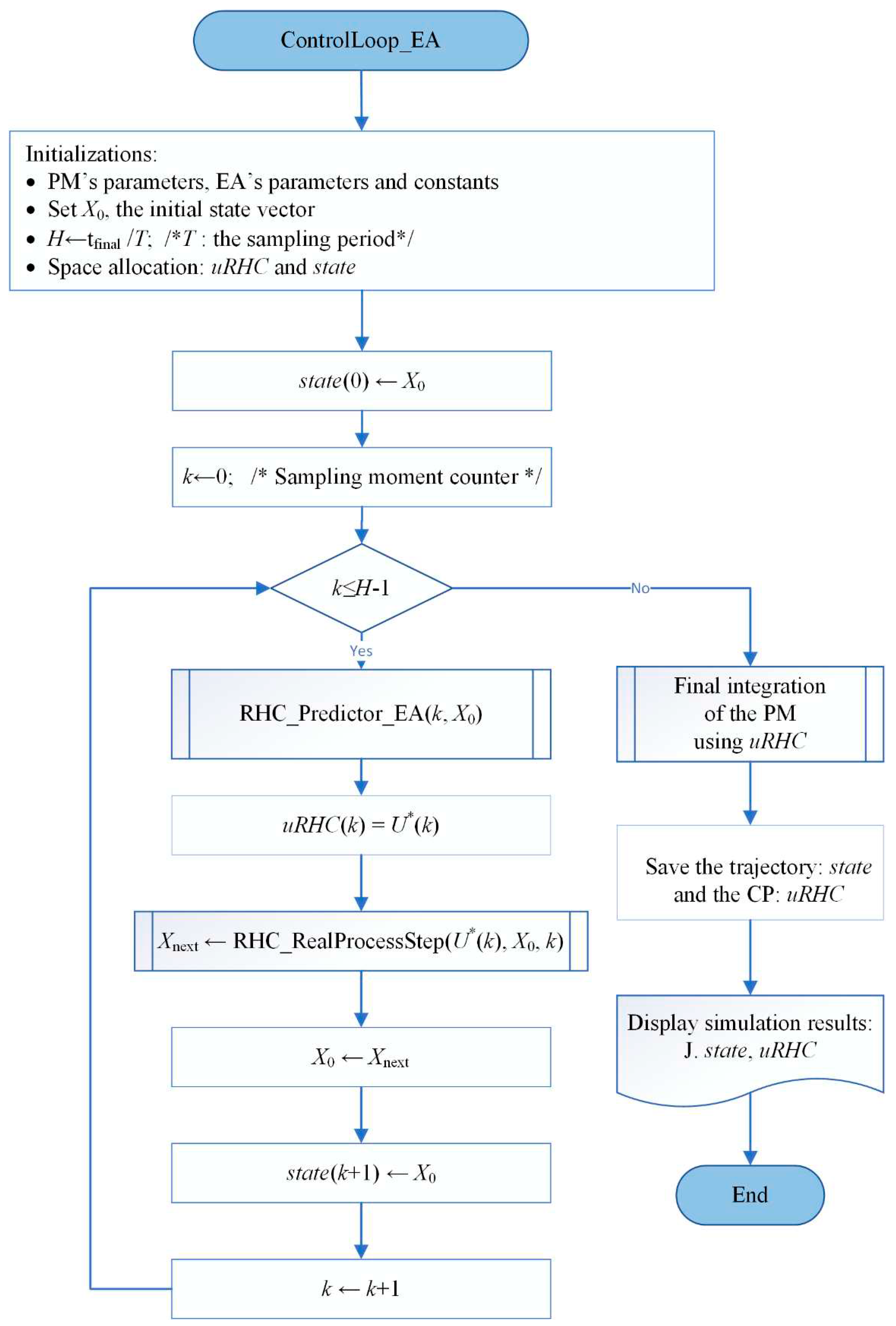
This subsection corresponds to step 1 of the design procedure. Figure 4 shows the flowchart of the simulation program for the closed loop (the script ControlLoop_EA.m).

At every moment k, the controller calls the predictor based on the EA, RHC_Predictor_EA. The last one returns the optimal control value

U^{*} (k)

, which is used by the function RHC_RealProcessStep to determine the next Process’s state.

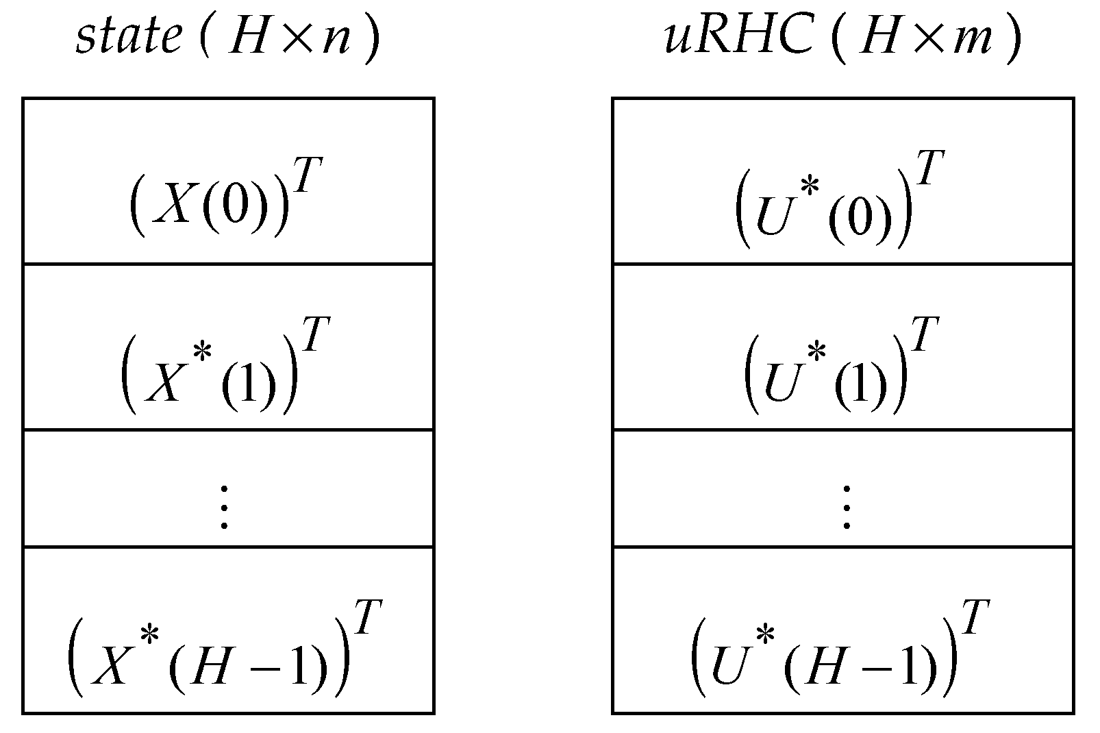
The optimal control value and the optimal states are stored in the matrices uRHC (H x m) and state (H x n), respectively, having the structure presented in Figure 5.

Hence, the optimal CP and trajectory are described by the matrix uRHC and state, respectively, which are the images of

Ω (X_{0})

and

Γ (X_{0})

sequences (see (12) and (13)).

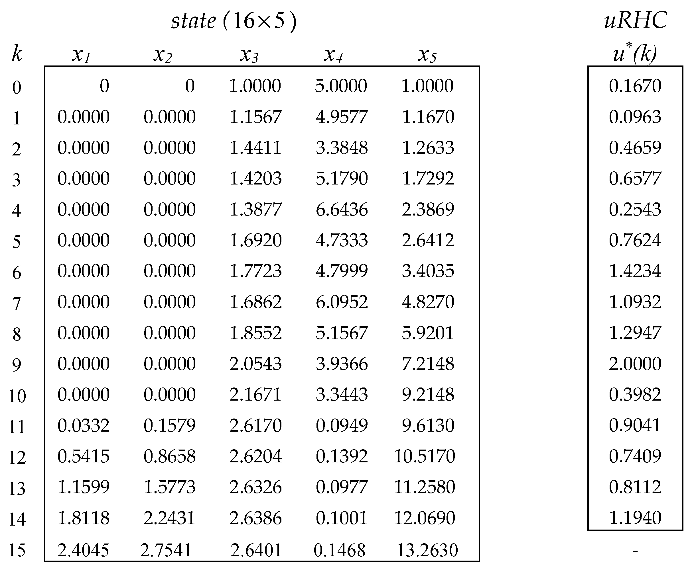
In the case of the PRP, an example of matrices describing a quasi-optimal evolution is given in Figure 6. Notice that, this time, m=1 and the 16th state is the final one.

3.2.2. Aggregation of datasets concerning M optimal evolutions of the closed loop

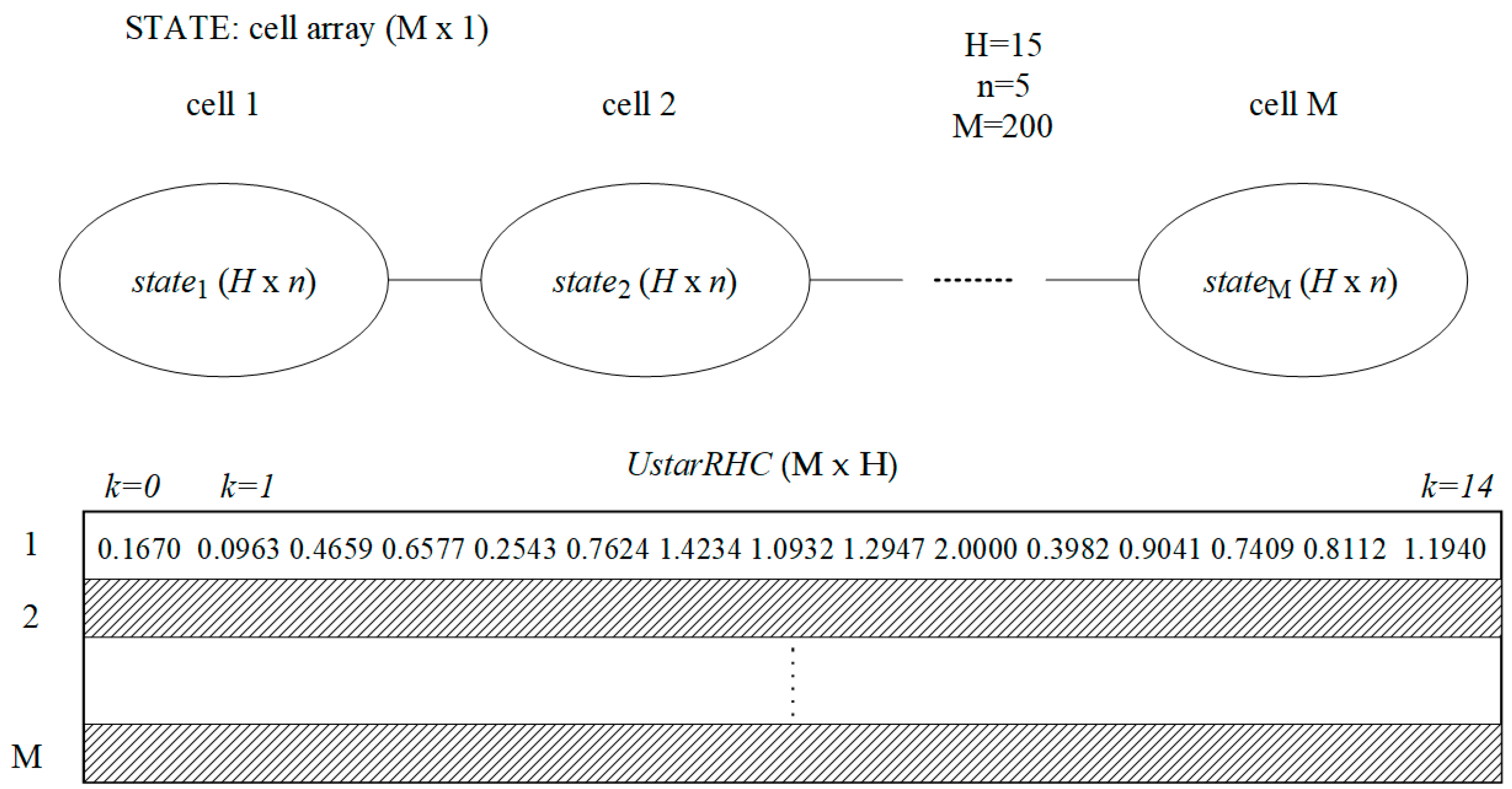
This subsection corresponds to step 2 of the design procedure. The controller’s optimal behaviour learning process needs data from an important number of optimal evolutions. Practically, the program ControlLoop_EA.m will be executed repeatedly M times (e.g. M=200) in a simple loop described in the script LOOP_M_ControlLoop_EA.m. The objective is to create aggregate data structures and store the optimal trajectories and their CPs.

Figure 7 illustrates possible data structures, a cell array for M tables storing the trajectories and a matrix storing their CPs.

The optimal CPs could also be stored in a cell array, but in the PRP case (m=1), a matrix (MxH) can store these values simpler. We call it UstarRHC (200 x 15); on each line, it memorizes the transposed vector uRHC from Figure 6.

The performance index values are also stored in a column vector JMAT (M x 1) for different analyses. All these data structures could be saved in a file for ulterior processing.

3.2.3. Extraction of datasets characterizing each sampling period

This subsection details step 3 of the design procedure. For each sampling period k, a dataset similar to Table 1 is extracted from STATE and UstarRHC data structures.

Considering k,

0 \leq k \leq H - 1

, is already fixed, we generate a matrix

S O C S K \in R^{M \times (n + m)}

that gathers the states and optimal control values concerning step k from all the M experiences. Line i,

1 \leq i \leq M

, concatenates data from experience i:

S O C S K_{i} \leftarrow [{(X_{i}^{*} (k))}^{T} {(U_{i}^{*} (k))}^{T}] .

Using the data structures defined before, it holds:

S O C S K_{i} \leftarrow [S T A T E_{i} (k, 1 : n) U s t a r R H C (i, k)] .

STATE_i designates the i^th component of the cell array STATE. In the PRP case, we have:

S O C S K = [\begin{array}{l} x_{1} {(k)}^{1} & x_{2} {(k)}^{1} & x_{3} {(k)}^{1} & x_{4} {(k)}^{1} & x_{5} {(k)}^{1} & u {(k)}^{1} \\ \dots & \dots & \dots & \dots & \dots & \dots \\ x_{1} {(k)}^{i} & x_{2} {(k)}^{i} & x_{3} {(k)}^{i} & x_{4} {(k)}^{i} & x_{5} {(k)}^{i} & u {(k)}^{i} \\ \dots & \dots & \dots & \dots & \dots & \dots \\ x_{1} {(k)}^{M} & x_{2} {(k)}^{M} & x_{3} {(k)}^{M} & x_{4} {(k)}^{M} & x_{5} {(k)}^{M} & u {(k)}^{M} \end{array}] .

Remark 5.

Because the Controller’s optimal behaviour has repercussions on each sampling period, the learning of its optimal behaviour will be split at the level of each interval [k, k+1).

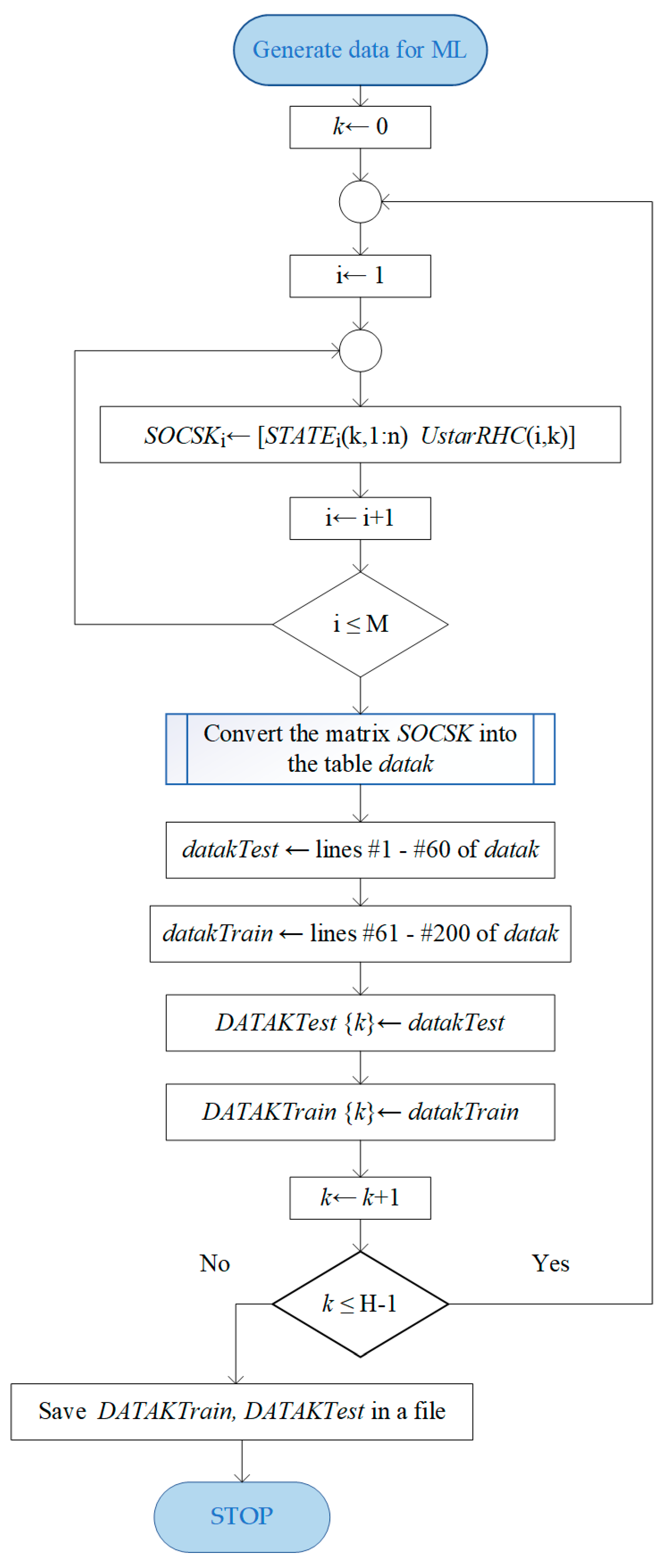
Figure 8 gives the flowchart of the data processing to obtain datasets for training and testing the machine learning algorithm at the level of each moment k (datakTrain and datakTest). To save these datasets for each k, we will use cell array DATAKTrain (

H \times 1

) and DATAKTest (

H \times 1

After constructing the matrix SOCSK, we shall convert it into a table, which seems more convenient for processing datasets for machine learning in some programming and simulation systems. The result is the table named datak, which has variables and properties. After that, this table’s lines are split into table datakTrain with 140 examples for training (70%) and table datakTest with 60 data points for testing (30%). Finally, these tables are stored in cell #k of the DATAKTrain and DATAKTest array, respectively. They will be used by the machine learning algorithm ulteriorly.

3.3. Construction of Machine Learning Models

This section covers step #4 of the design procedure. As stated by Remark 3, the set of functions

Φ = {f_{k} |k = 0, 1, \dots, H - 1}

is the machine-learning model for the optimal behaviour of the couple (PM – EA). The data points are couples (Process state – optimal control values) related to moment k, which the function

f_{k}

can learn.

Of course, another kind of machine-learning model treating globally the learning process (PM – EA’s control profile) could be addressed, without splitting the learning at the level of sampling periods. The resulting model would be more complex and difficult to train and integrate into the controller.

In this work, we mainly chose multiple linear regression as a machine learning algorithm because of its simplicity. This characteristic is important, especially when H is large. Secondly, the linear regression functions

f_{k}

for each sampling period are appropriate for a controller implementation; these functions directly give the control law (see equation (14)). To emphasize this aspect, Table 2 presents the general structure of the ML_controller when using the set of functions

Φ

We could determine the set of functions

Φ

through multiple linear regression considering different models containing an intercept, linear terms for each feature (predictor variable), products of pairs of distinct features (interactions), squared terms, etc. In other words, the resulting functions could be nonlinear as functions of Process states.

In our case study, we will also apply the strategy of stepwise regression that adds or removes features starting from a constant model.

3.3.1. Models with linear terms for each state variable

Remark 6.

Our objective is not to find the “best” set of linear regression models but to prove that our approach is working and this new model can replace the EA.

That is why, for the beginning, we adopt a very simple model such that each regression function

f_{k}

is a simple linear model involving only linear terms for each state variable and an intercept. Each model is trained and tested separately, considering the datasets already prepared in the cell arrays DATAKTrain and DATAKTest.

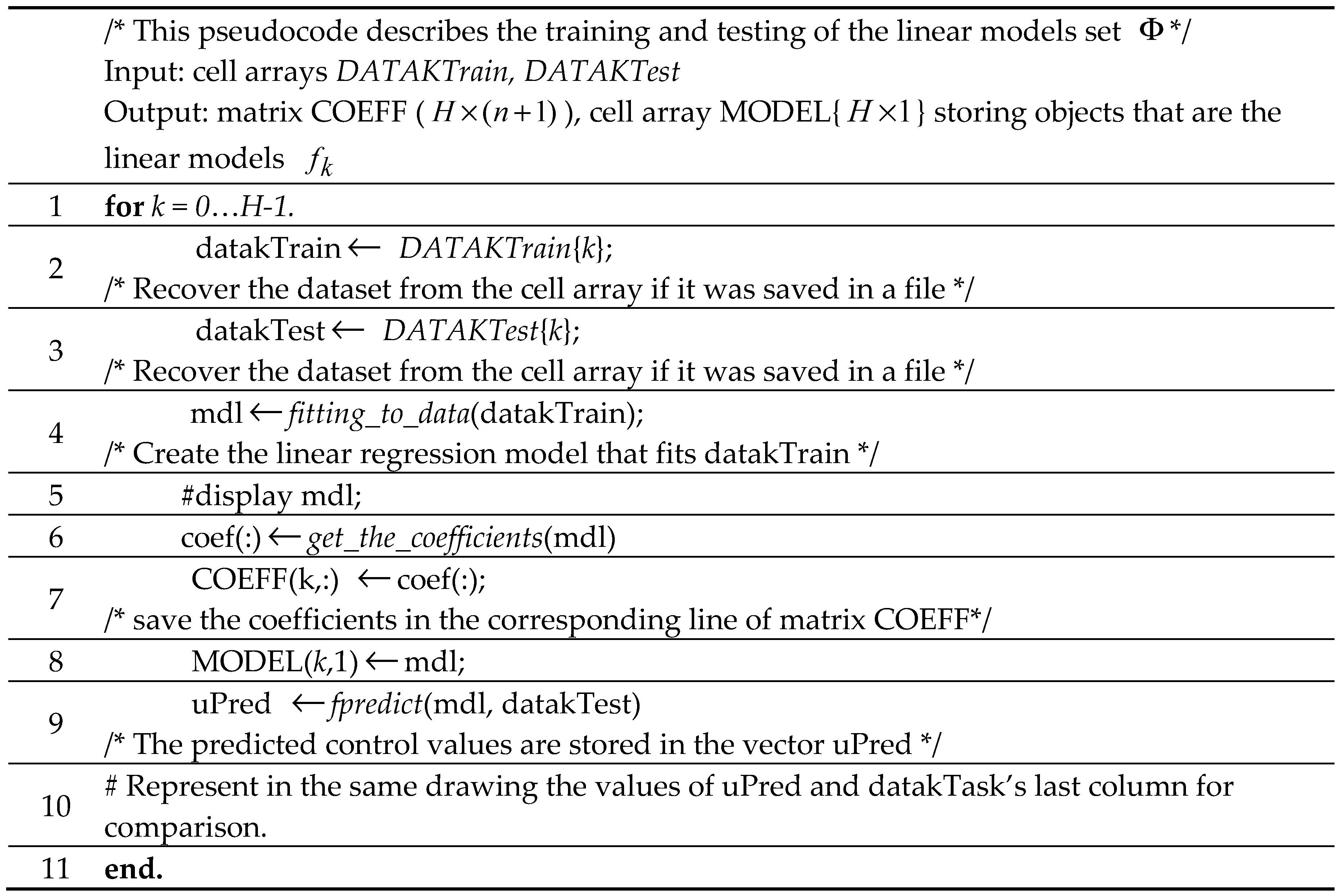
The construction of these models is presented by the pseudocode in Table 3. The datasets for training and testing, described in section 3.2.3, are now input data for this algorithm. The coefficients of each function

f_{k}

, having the form

f_{k} (X (k)) = C^{k}_{0} + C^{k}_{1} \cdot x_{1} (k) + C^{k}_{2} \cdot x_{2} (k) + \dots + C^{k}_{n} \cdot x_{n} (k),

(15)

are stored in an output matrix called COEFF. These models are objects stored in an output cell array called MODEL (

H \times 1

). Line #4 creates the model “mdl” using the function fitting_to_data that fits the function (15) to the dataset “datakTrain”. At line #6, the function get_the_coefficients extracts the six coefficients, which are put in a line of matrix COEFF afterwards.

The predicted values corresponding to datakTest are stored in the vector “uPred” by the function fpredict to be compared with the experienced values. Details concerning the implementation of fitting_to_data, get_the_coefficients, and predict functions are given in Appendix B.

For the PRP, e.g., the coefficients are given in Table B2 (Appendix B).

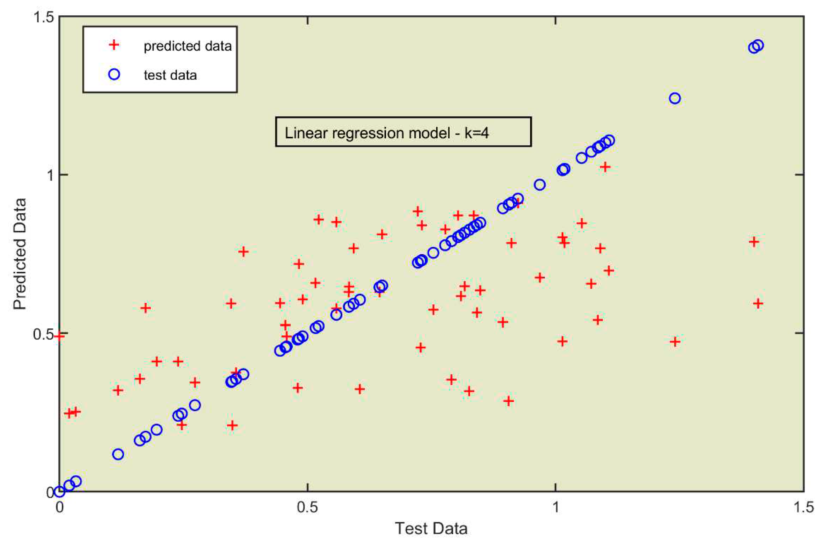
A comparison of the values in “datakTest” to the predicted values “uPred” is given in Figure 9 [29,31]. The blue line is the plot of test values against themselves.

The 60 predicted values are disposed along the blue line at a distance inferior to 0.2 for most of them.

3.3.2. Models constructed through stepwise regression

This section will propose a more elaborate model that allows the possibility to include nonlinear terms as the interactions, that is, the product of predictor variables (ex.: x₁*x₄).

As an example, for the PRP case, we will apply the strategy of stepwise regression that adds or removes features starting from a constant model. This strategy is usually implemented by a function stepwise(T) returning a model that fits the dataset in Table T.

model \leftarrow stepwise (T)

The script GENERATE_ModelSW.m constructs de set of models using this function (see Appendix C). This script yields the regression functions given in Table 4.

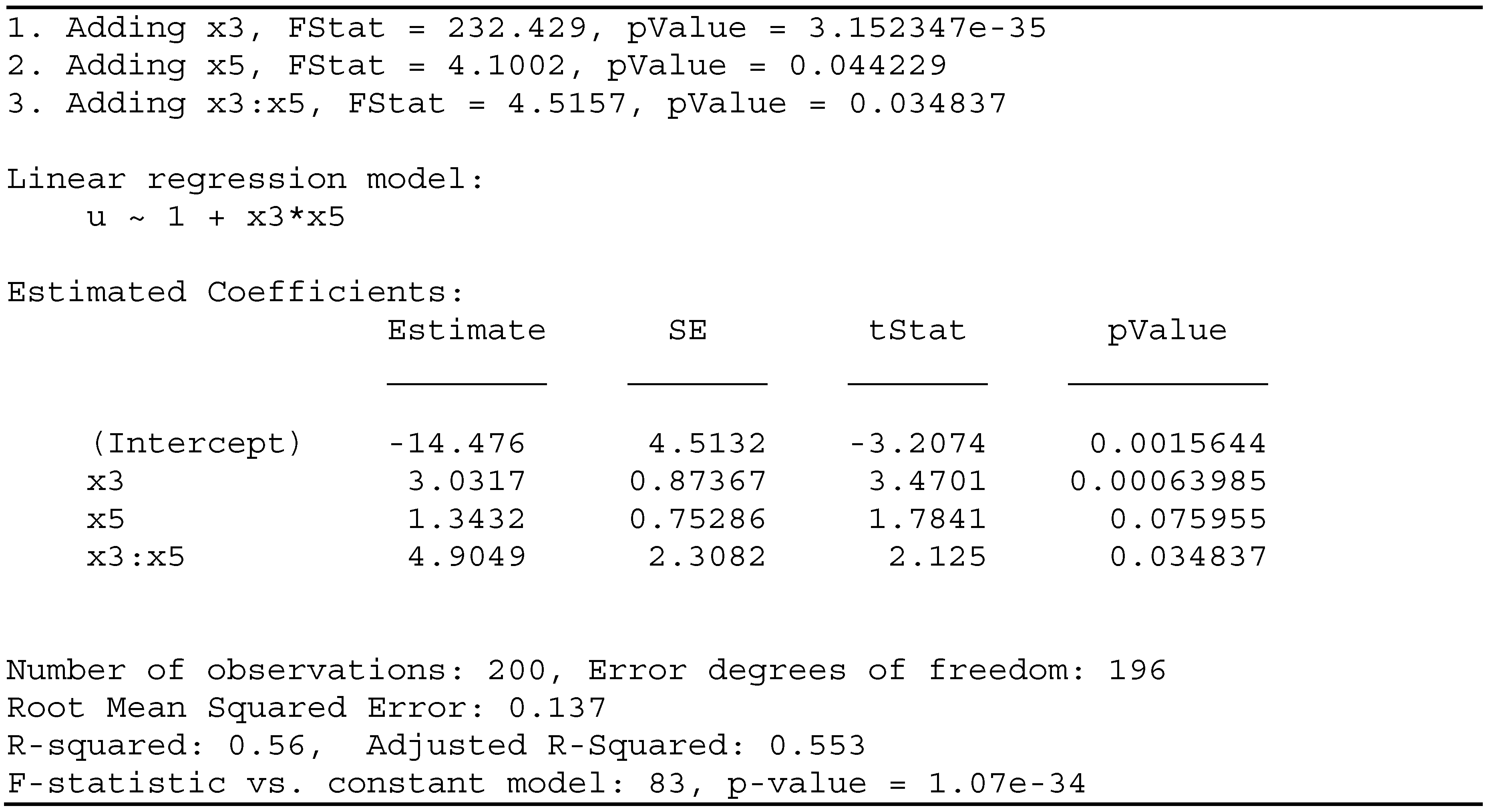
A fragment of the listing generated by the script mentioned above is given in Table 5.

We can see how the function stepwise works and what are the statistic parameters that validate the model.

4. Simulation of the control-loop system equipped with the ML_controller

To evaluate the measure in which the set of functions

Φ

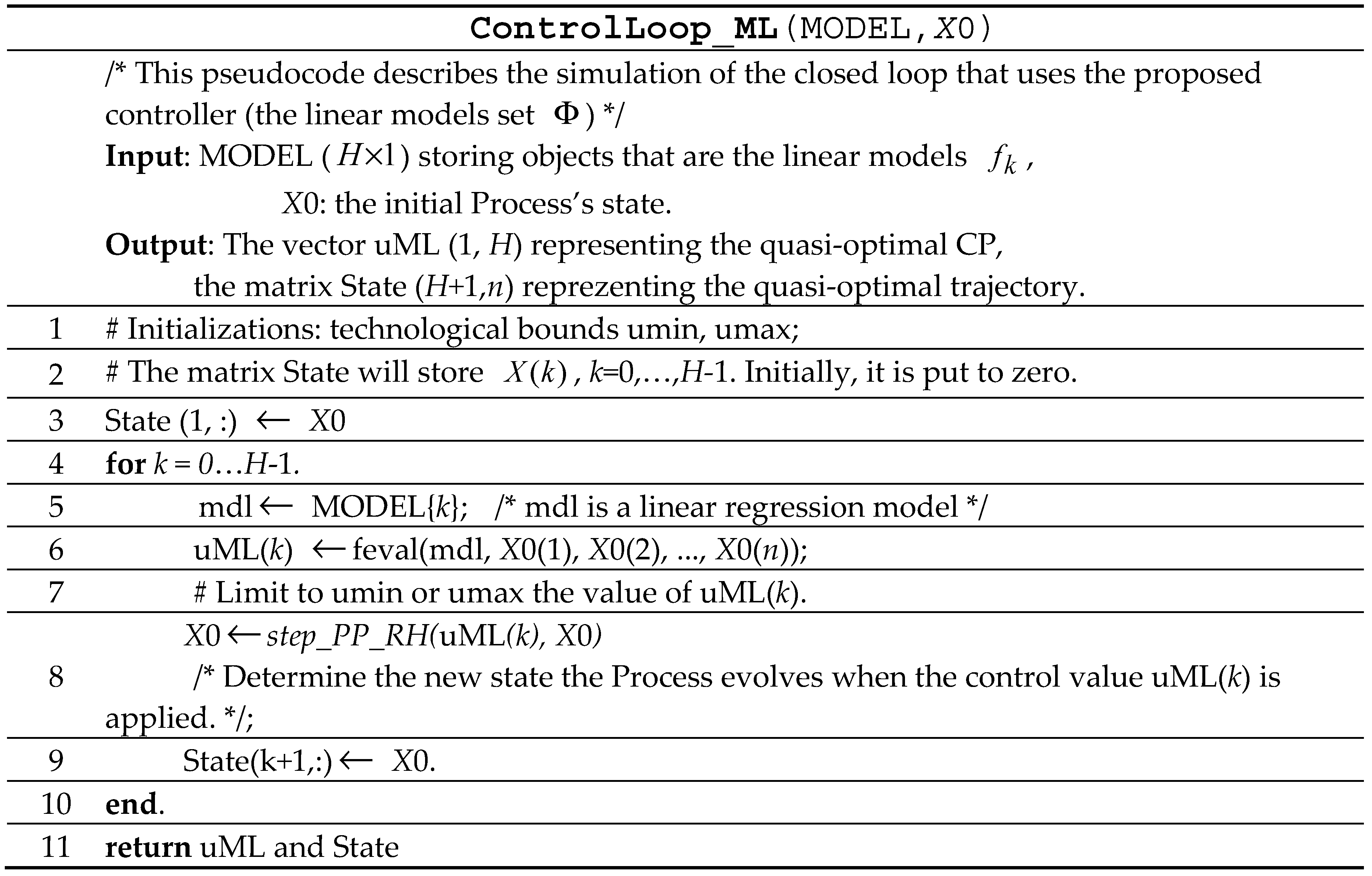
succeeded in “learning” how the EA acts as an optimal predictor, we shall refer to the simulation results of the control loop. The script ControlLoop_ML.m implements step #6 of the design procedure and is described by the pseudocode in Table 6.

In line #6, the function feval returns the value uML(k) that the model mdl predicts when the current state is X0 (also a local variable). Instead of using feval, one can use the product coefficients - state variable.

The function step_PP_RH(uML(k), X0) calculates the next state (at the moment k+1) by integration of state equations (7). The codes for all the proposed functions are given in the folder ART_Math.

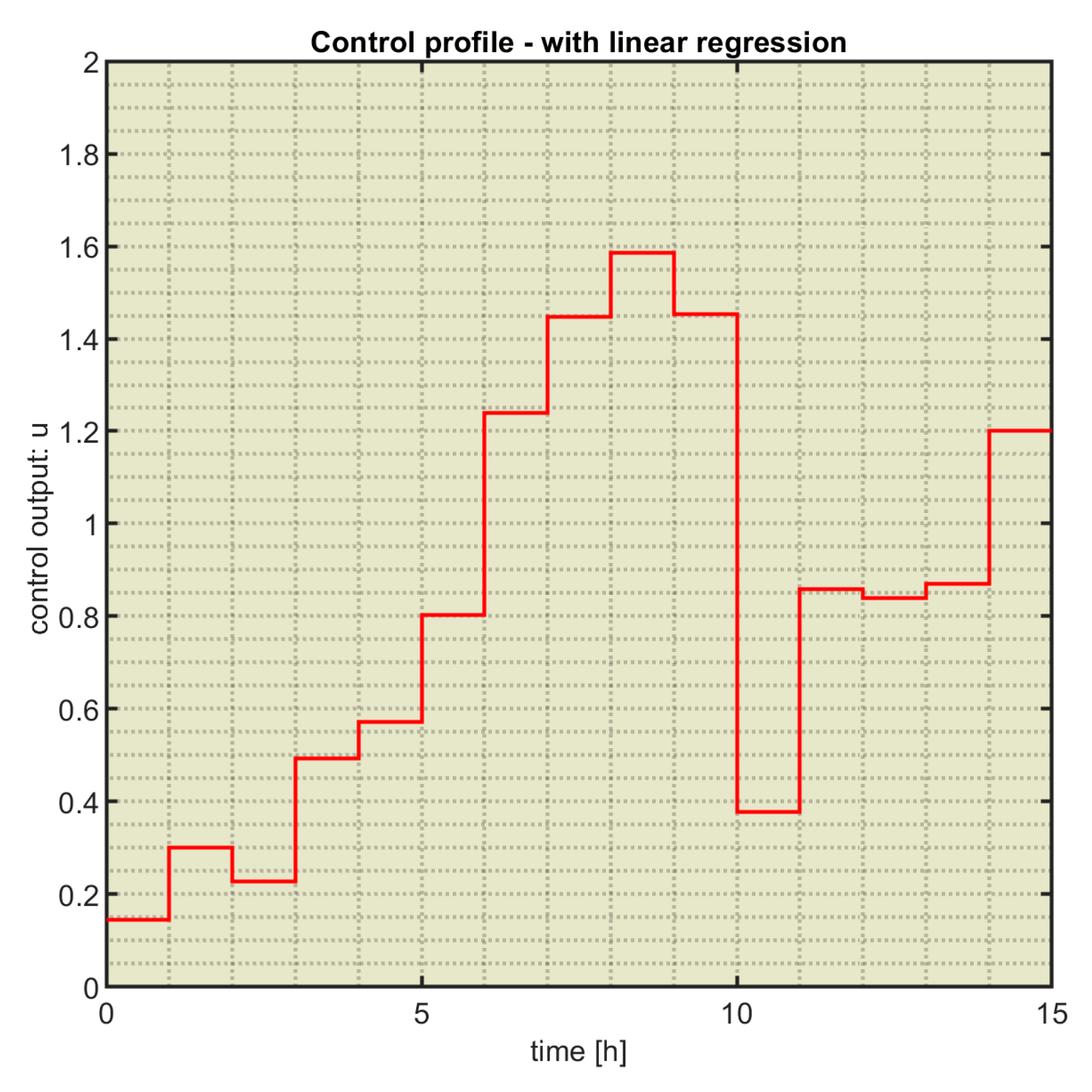
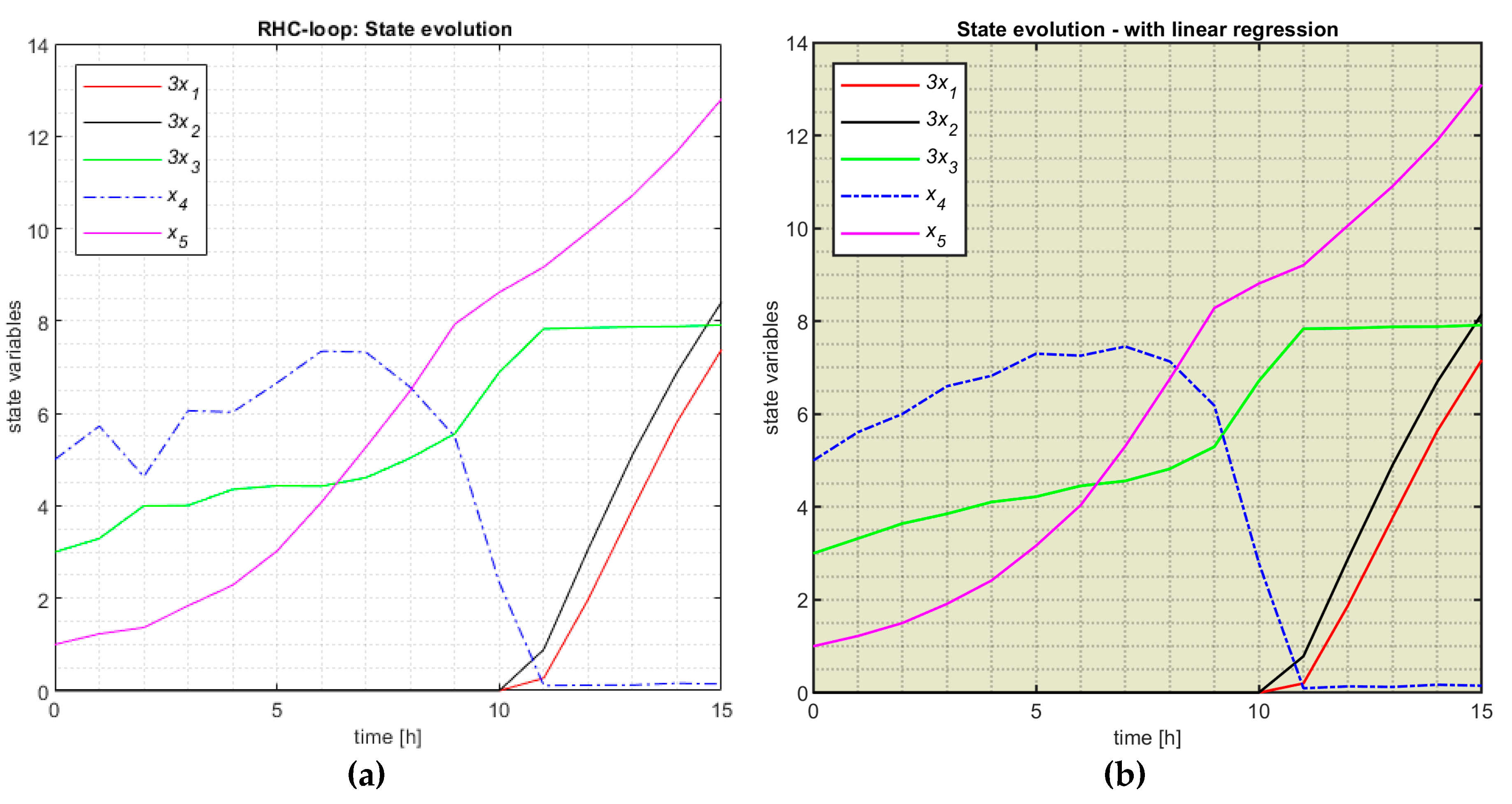
In the PRP case, we used ControlLoop_ML.m to simulate the control loop using the models constructed in section 3.3.1. The ML_controller yielded the CP drawn in Figure 10. This one engenders the quasi-optimal state evolution depicted in Figure 11b, which can be compared to the typical evolution, Figure 11a, generated by the RHC endowed with an EA. Figure 11a was produced within the authors’ previous work [21].

The resemblance between the two process’s responses is very high and proves that the set of functions

f_{k}

succeeded in emulating the optimal behaviour of the EA. Moreover, the performance index’s value achieved by the CP in Figure 11b is very good

J_{0} = 32 . 0986

because it equals the maximum value (J₀=32.0936) recorded in the M data points generated by the EA. Hence, the PRP’s solution found by the ML model is also quasi-optimal.

The controller’s execution time

Because the initial reason for this research is just the EA’s execution time decrease, we compared the execution time of the two controllers, the EA and ML controllers. Actually, we compared the simulation times for the two closed loops with the EA and ML models because we already have the programs ControlLoop_EA.m and ControlLoop_ML.m.The two times are 38 seconds and 0.08 seconds, respectively (see Appendix D). The average execution times of the controller are 38/H and 0.08/H seconds. H equals 15 in the PRP case.

Remark 7.

The decrease in the controller’s execution time is outstanding, all the more so because the ML_controller keeps the evolution accuracy. In anterior research, we have obtained a small decrease but with an acceptable accuracy decrease as well.

How can we explain this outstanding decrease in the controller’s execution time? The key is how the EA predictor works. The EA algorithm generates a population of solutions and then evaluates the cost function by numerical integration of the PM for each solution and along many generations. The PM’s numerical integration for thousands of times is the most time-consuming. Nothing of these happens when the ML model works, only a single evaluation of a simple regression function. The EA’s computational complexity is huge compared to a few calculations.

The model developed in section 3.3.2

Φ_{2}

(considering

Φ_{1}

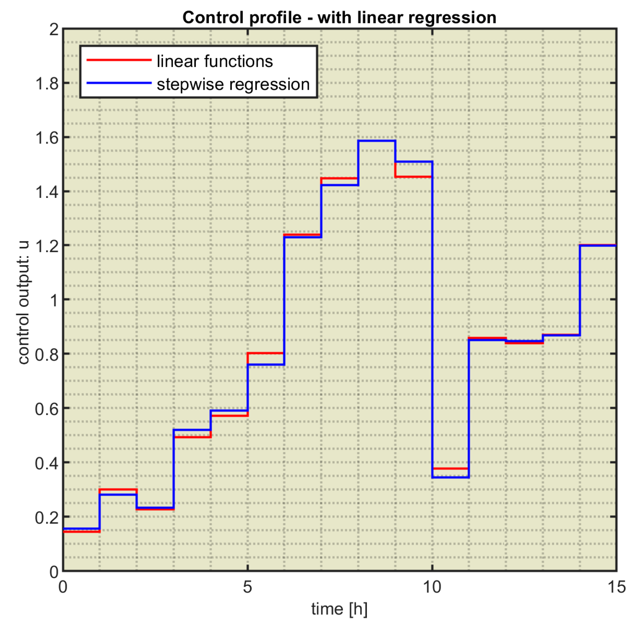
the model constructed in section 3.3.1) leads us to a new ML controller. This time, we used the script ControlLoop_MLSW.m (see Appendix C) to simulate the closed-loop system. Figure 12 plots the resulting CP in a blue line. The CP in Figure 10 is also plotted in red to facilitate the comparison.

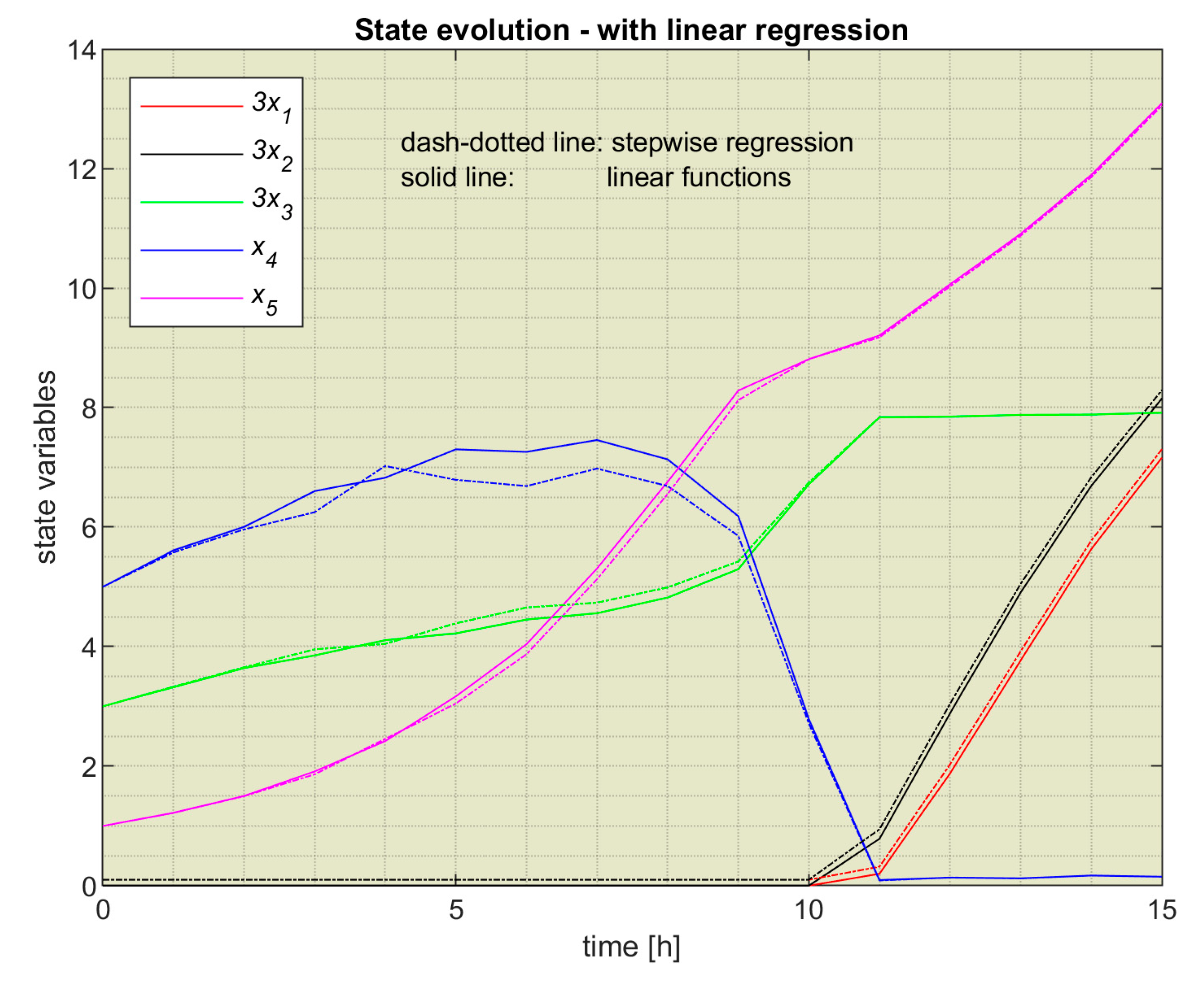
The two CPs are practically identical, which will engender the similarity of the state evolutions. Figure 13 confirms that situation and plots the state evolutions involved by the two controllers.

This remarkable similarity is because the models

Φ_{1}

and

Φ_{2}

emulate the same couple (EA-PM), and both do it very well. Consequently, the performance index is practically the same (

J_{0} = 32 . 0986

). Although the results are identical, the sets of regression functions are different. The functions set

Φ_{2}

seems more appropriate for the controller’s implementation because of their simpler formulas.

In real-time, the difference between the PM’s state and the state of the process is the biggest problem. We can consider that the Process is affected by a noise representing this difference. When the noise is important, the control loop could loose totally its functionality. Our desideratum is that the controller keeps acceptable performances for a significative noise range. Inside this range, the controller must reject this difference as much as possible, involve a quasi-optimal process evolution, and produce a performance index near J₀ (see Appendix E).

5. Discussion

This paper answers positively to the issue raised in section 1: whether an ML algorithm could “learn” the optimal behaviour of the predictor based on an EA. The proof was made in the context of OCPs, giving rise to some findings:

The issue statement oneself: to find an ML model experiencing the datasets generated by the couple (EA -PM), trying to capture its optimal behaviour. An EA is a product of computational intelligence. This link between two “intelligent” entities is interesting; further developments can be derived from this “equivalence”. The same issue can be considered when instead of EA is another metaheuristic.
The dataset’s construction as a dynamic trace of the EA predictor by aggregating the trajectories and CPs. The number M is a procedure’s parameter established according to the process complexity. The dynamic trace must include couples (state, optimal control value) spread throughout the evolution space. In this way, the ML model could generalize well.
The dataset extraction for each sampling period, which is a premise to find an ML model for each k.
The outstanding decrease in the ML_controller’s execution time.
The design procedure for the ML_controller and all associated algorithms (simulation and models’ construction algorithms).

Finding #3 is related to the fact that we are looking for an ML model comprising a set of regression functions

Φ

. We underline the motivation: its simplicity, especially when the control horizon has many sampling periods. If need be, obtaining the model during the sampling period is conceivable. On the other hand, a regression function for each sampling period means that the control law is directly implemented. The controller implementation is now straightforward.

The degree to which the ML_controller accurately reproduces the couple (EA, PM)’s behaviour outclasses another achievement of the controller: its execution time. Because the initial reason for this research is just the EA’s execution time decrease, this subject deserves more attention. The simulation time for the closed loop using the EA predictor for the PRP case is 38 seconds, while the same simulation using the ML_controller is 0.08 seconds. This outstanding achievement is due to three factors:

the ML model is split at the level of each sampling period; a single regression function $f_{k}$ is the current model;
a regression function has a very simple expression, which is, in fact, just the control law.
the PM’s numerical integration is totally avoided.

According to the authors’ experience addressing this subject, the execution time decrease to a small extent is done by paying the price of predictions’ accuracy decrease as well. In the case of the ML_controller, remarkably, that does not happen; the accuracy is kept.

As we mentioned before, predictors based on metaheuristics are usually used for slow process control. Owing to its small execution time, the ML_controller extends largely the set of processes, which can be controlled using EA or another metaheuristic. We must implement the EA predictor in the first phase of the controller’s design, which will produce the datasets for the ML algorithm’s training. Finally, the ML predictor will be used as a faster equivalent of the EA predictor in the control structure.

Special attention was addressed to the implementation aspects related to the PRP case. All algorithms used in this work are implemented, the associated scripts are attached as supplementary materials, and all the necessary details are given in the Appendixes. Readers can find support to apprehend and eventually reproduce parts of this work.

Finally, the ML models and the controller must fulfil their task in real conditions, namely when the control system works with a real Process. Although the design procedure does not depend on the real Process, an interested reader can ask how to forecast the closed-loop behaviour when the real Process and the PM differ. At the end of section #4 and in Appendix D, some elements can help to simulate this situation.

To simplify the presentation, we applied the proposed methods only in the PRP case. The methods were also applied in other case studies not presented in this paper, with the same favourable conclusion; the proposed ML models succeeded in apprehending the optimal behaviour of the couple (EA, PM) and yielded efficient controllers.

Obviously, another ML model treating globally the learning process is conceivable, without splitting the learning at the level of sampling periods. The resulting model would be more complex and difficult to train and integrate into the controller, but it could be useful in other applications. In a further research project we will make investigations in this direction.

Author Contributions

Conceptualization, V.M.; methodology, I.A. and V.M.; software, V.M.; validation, V.M. and I.A.; formal analysis, V.M.; investigation, I.A.; resources, I.A.; data curation, I.A.; writing—original draft preparation, V.M.; writing—review and editing, V.M. and I.A.; visualization, I.A.; supervision, I.A.; project administration, I.A.; funding acquisition, I.A. All authors have read and agreed to the published version of the manuscript.

Funding

This research received no external funding.

Data Availability Statement

No new data were created.

Acknowledgments

This work benefited from the administrative support of the Doctoral School of “Dunarea de Jos” University of Galati, Romania.

Conflicts of Interest

The authors declare no conflict of interest.

Appendix A

The prediction function using an EA

Figure A1. The flowchart of the prediction function using an EA (RHC_Predictor_EA.m).

The cost function values of the offspring are calculated inside the EA’s operators. Variable F is used to stop the iterative process toward the optimal solution. When the performance index is close to J₀, the EA stops, considering that a very good solution is found, and the best solution becomes the predicted control sequence.

Appendix B

The models’ construction script

Our implementation is based on the MATLAB system, in which “fitlm”, “model.Coefficients”, and “predict” correspond to fitting_to_data, get_the_coefficients, and fpredict (the functions proposed in section 3.3.1), respectively. The algorithms in Figure 8 and Table 2 are joined and implemented by the script Model_Construction.m. The coefficients found by the script Model_Construction.m are listed in the table below.

Table B1. The regression functions following the stepwise strategy.Table 5. Construction of the regression model by stepwise function for k=2.Table 6. The pseudocode of the control loop simulation using linear regression functions.Table B1. The coefficients of the linear regression f_k.

k	C0	C1	C2	C3	C4	C5
	_______	_________	_________	_______	________	________
0	-38.079	0	0	14.128	6.0244	-6.0264
1	5.6291	-1.3608^e+07	2.4367^e+06	-3.7392	-0.47639	1.139
2	-38.33	3.0713^e+05	-2.2759^e+05	21.679	1.5663	1.8422
3	-28.268	-40144	4487.7	14.638	1.1171	1.2135
4	-29.163	1.6973^e+05	-1.6184^e+05	14.311	1.2206	0.63983
5	-88.374	95097	-1.0768^e+05	40.145	4.0721	0.78088
6	-25.715	3.5858^e+05	-3.7572^e+05	13.047	1.5373	-1.0067
7	-62.516	-4.657^e+05	4.4453^e+05	29.336	4.0186	-2.0782
8	45.254	-1.387^e+07	1.3915^e+07	-13.445	-0.83017	-2.415
9	504.78	-2.211^e+06	2.2891^e+06	-192.32	-23.957	-1.8747
10	-236.04	-82.588	11.879	95.084	12.898	-1.3842
11	-147.92	0.58548	0.29874	57.825	7.5075	-0.34759
12	93.46	-0.37731	-0.76193	-35.138	-4.7889	0.094402
13	34.849	-1.0111	0.66035	-13.353	-0.79003	0.1234
14	4.0848	-0.30413	0.29959	-1.6444	-0.43335	0.11348

Appendix C

Implementation of the stepwise strategy

The stepwise strategy is implemented through the function “stepwiselm”, which adds or removes terms to the current model. The set of available terms is addressed, and the one having an F-test for adding it with a p-value of 0.05 or less is added to the model. If no terms can be added, the function evaluates the terms in the model and removes that one having an F-test for removing it with a p-value of 0.10 or greater. This process stops when no terms can be added or removed.

The models from section 3.3.2 are generated using this function for each k in the script GENERATE_ModelSW.m. The latter has the same structure as Model_Construction.m, except the function stepwiselm is used instead of fitlm.

To simulate the closed loop, we used the script ControlLoop_MLSW.m, which is very similar to ControlLoop_ML.m but uses a different mat-file. Finally, it calls the script DRAW_ML to plot the CP and the state evolution.

Appendix D

Execution time

Because the ControlLoop_ML is conceived as a function, the closed loop simulation is made by the script SIM1.m, which calls it after loading the ML model. The simulation processor is IntelI CoreI i7-6700HQ CPU @ 2.60GHz.

Finally, the comparison is made between the execution time of two programs, ControlLoop_EA.m and SIM1.m. The results are 38 seconds and 0.8 seconds, respectively.

Appendix E

The ML_controller’s capacity to reject noises affecting the Process state

The general problem of noise modelling depends on the Process specificity and overpass the aim of this work. Our immediate goal is to provide a simple technique to test the existence of a noise range where the controller keeps acceptable performances.

In our simulation, we considered the noise is added to the PM’s state variables. For our example, the noise I

n_{i}

, equivalent to all influences, is added to the PM’s vector state:

x_{i} (k) \leftarrow x_{i} (k) + n_{i}, i = 1, \dots, 5

We adopted the hypothesis the noise is a random variable RT in the interval [-L_i, L_i], where

L_{i} = p \cdot |x_{i} (k)|, 0 < p < 1

Hence, the noise depends on the state variable’s absolute value to avoid annulling its influence. We have chosen a constant value of 4%, which means an 8% interval for placing the noise. The controller keeps the regression models from Table 5.

These elements have been inserted into the control loop simulation script (ControlLoop_ML_noise.m), which has been carried out many times. Table 6 presents only three CPs and the associated performance index to evaluate whether the control loop has a margin of robustness to noise.

Table E1. Three simulations of the control loop with noise.

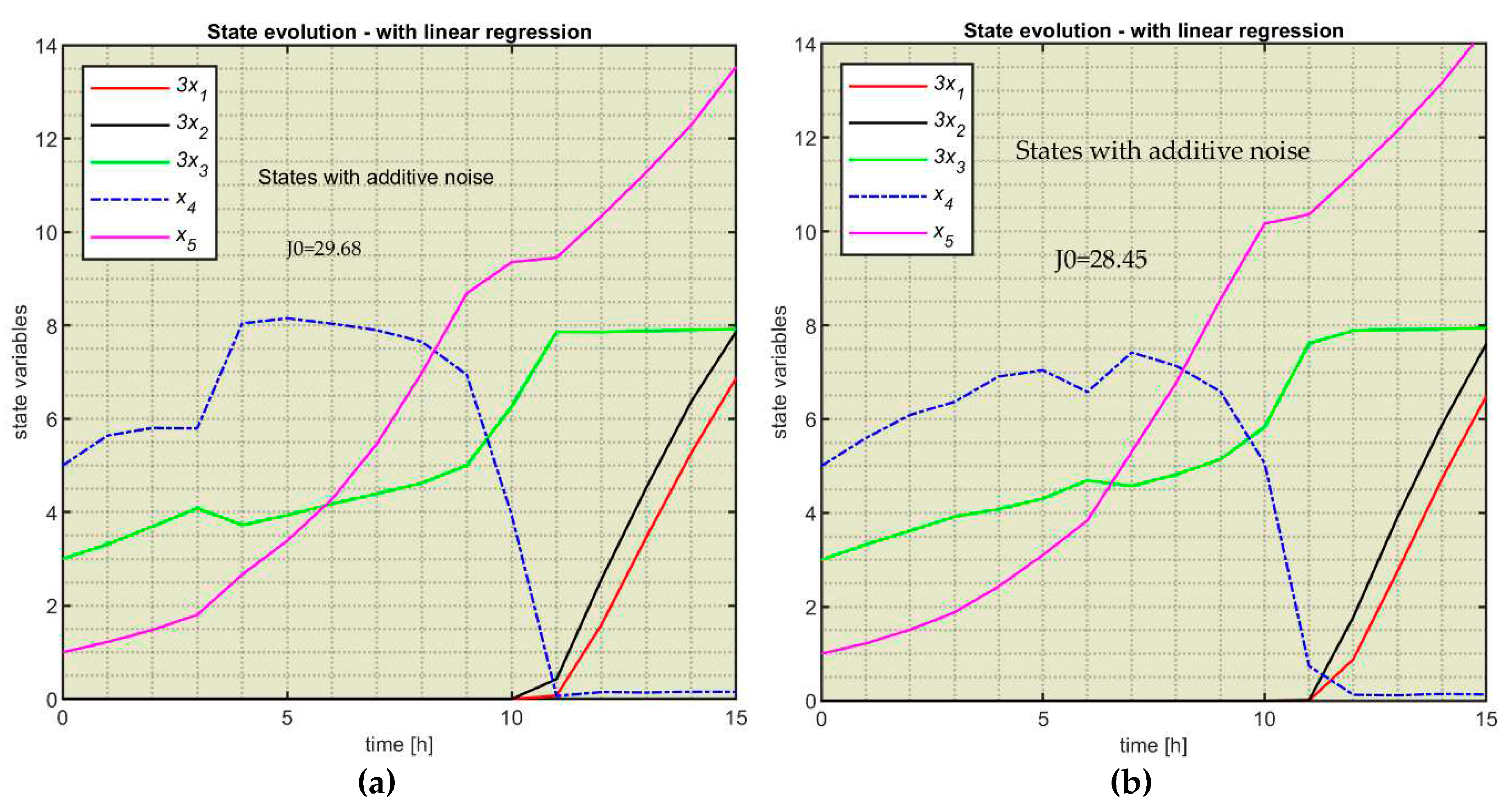
The state evolution for the two first simulations is presented in Figure E1.

After simulations, some conclusions can be drawn:

-: The controller succeeded in keeping the stability, but the state evolution changed the look compared to Figure 11b.
-: The value $J$ is generally smaller than $J_{0}$ and has different values for different simulations because the noise has random values.
-: Technological aspects must be considered when deciding whether or not the controller works acceptably.

References

Siarry, P. Metaheuristics; Springer: Berlin/Heidelberg, Germany, 2016; ISBN 978-3-319-45403-0. [Google Scholar]
Talbi, E.G. Metaheuristics—From Design to Implementation; Wiley: Hoboken, NJ, USA, 2009; ISBN 978-0-470-27858-1. [Google Scholar]
Kruse, R.; Borgelt, C.; Braune, C.; Mostaghim, S.; Steinbrecher, M. Computational Intelligence—A Methodological Introduction, 2nd ed.; Springer: Berlin/Heidelberg, Germany, 2016. [Google Scholar] [CrossRef]
Faber, R.; Jockenhövelb, T.; Tsatsaronis, G. Dynamic optimization with simulated annealing. Comput. Chem. Eng. 2005, 29, 273–290. [Google Scholar] [CrossRef]
Onwubolu, G.; Babu, B.V. New Optimization Techniques in Engineering; Springer: Berlin/Heidelberg, Germany, 2004. [Google Scholar]
Valadi, J.; Siarry, P. Applications of Metaheuristics in Process Engineering; Springer International Publishing: Berlin/Heidelberg, Germany, 2014; pp. 1–39. [Google Scholar] [CrossRef]
Minzu, V.; Riahi, S.; Rusu, E. Optimal control of an ultraviolet water disinfection system. Appl. Sci. 2021, 11, 2638. [Google Scholar] [CrossRef]
Minzu, V.; Ifrim, G.; Arama, I. Control of Microalgae Growth in Artificially Lighted Photobioreactors Using Metaheuristic-Based Predictions. Sensors 2021, 21, 8065. [Google Scholar] [CrossRef]
Abraham, A.; Jain, L.; Goldberg, R. Evolutionary Multiobjective Optimization—Theoretical Advances and Applications; Springer: Berlin/Heidelberg, Germany, 2005; ISBN 1-85233-787-7. [Google Scholar]
Hu, X.B.; Chen, W.H. Genetic algorithm based on receding horizon control for arrival sequencing and scheduling. Eng. Appl. Artif. Intell. 2005, 18, 633–642. [Google Scholar] [CrossRef]
Hu, X.B.; Chen, W.H. Genetic algorithm based on receding horizon control for real-time implementations in dynamic environments. Proceedings of the 16th Triennial World Congress, Prague, Czech Republic, 4–8 July 2005; Elsevier IFAC Publications: Amsterdam, The Netherlands, 2005. [Google Scholar]
Mayne, D.Q.; Michalska, H. Receding Horizon Control of Nonlinear Systems. IEEE Trans. Autom. Control. 1990, 35, 814–824. [Google Scholar] [CrossRef]
Mînzu, V.; Rusu, E.; Arama, I. Execution Time Decrease for Controllers Based on Adaptive Particle Swarm Optimization. Inventions 2023, 8, 9. [Google Scholar] [CrossRef]
Goggos, V.; King, R. ; Evolutionary predictive control. Comput. Chem. Eng. 1996, 20 (Suppl. 2), S817–S822. [Google Scholar] [CrossRef]
Chiang, P.-K.; Willems, P. Combine Evolutionary Optimization with Model Predictive Control in Real-time Flood Control of a River System. Water Resour. Manag. 2015, 29, 2527–2542. [Google Scholar] [CrossRef]
Minzu, V.; Serbencu, A. Systematic procedure for optimal controller implementation using metaheuristic algorithms. Intell. Autom. Soft Comput. 2020, 26, 663–677. [Google Scholar] [CrossRef]
Minzu, V. Quasi-optimal character of metaheuristic-based algorithms used in closed-loop — Evaluation through simulation series. Proceedings of ISEEE, Galati, Romania, 18 –. 20 October.
Minzu, V. Optimal Control Implementation with Terminal Penalty Using Metaheuristic Algorithms. Automation 2020, 1, 48–65. [Google Scholar] [CrossRef]
Minzu, V.; Riahi, S.; Rusu, E. Implementation aspects regarding closed-loop control systems using evolutionary algorithms. Inventions 2021, 6, 53. [Google Scholar] [CrossRef]
Minzu, V.; Arama, I. 2022. [CrossRef]
Minzu, V.; Georgescu, L.; Rusu, E. Predictions Based on Evolutionary Algorithms Using Predefined Control Profiles. Electronics 2022, 11, 1682. [Google Scholar] [CrossRef]
Goodfellow, I.; Bengio, Y.; Courville, A. , Machine Learning Basics. In Deep Learning, 2016. [Google Scholar]
Zou, S.; Chu, C.; Shen, N.; Ren, J. Healthcare Cost Prediction Based on Hybrid Machine Learning Algorithms. Mathematics 2023, 11, 4778. [Google Scholar] [CrossRef]
Cuadrado, D.; Valls, A.; Riaño, D. Predicting Intensive Care Unit Patients’ Discharge Date with a Hybrid Machine Learning Model That Combines Length of Stay and Days to Discharge. Mathematics 2023, 11, 4773. [Google Scholar] [CrossRef]
Albahli, S.; Irtaza, A.; Nazir, T.; Mehmood, A.; Alkhalifah, A.; Albattah, W. A Machine Learning Method for Prediction of Stock Market Using Real-Time Twitter Data. Electronics 2022, 11, 3414. [Google Scholar] [CrossRef]
Wilson, C.; Marchetti, F.; Di Carlo, M.; Riccardi, A.; Minisci, E. Classifying Intelligence in Machines: A Taxonomy of Intelligent Control. Robotics 2020, 9, 64. [Google Scholar] [CrossRef]
Banga, J.R.; Balsa-Canto, E.; Moles, C.G.; Alonso, A. Dynamic optimization of bioprocesses: Efficient and robust numerical strategies. J. Biotechnol. 2005, 117, 407–419. [Google Scholar] [CrossRef] [PubMed]
Balsa-Canto, E.; Banga, J.R.; Aloso, A.V. Vassiliadis. Dynamic optimization of chemical and biochemical processes using restricted second-order information 2001. Comput. Chem. Eng. 2001, 25, 539–546. [Google Scholar]
Newbold, P.; Carlson, W.L.; Thorne, B. Multiple Regression. In Statistics for Business and Economics, 6th ed.; Pfaltzgraff, M, Bradley, A., Eds.; Publisher: Pearson Education, Inc., New Jersey, 07458, USA, 2007. [Google Scholar]
Shi, H.; Zhang, X.; Gao, Y.; Wang, S.; Ning, Y. Robust Total Least Squares Estimation Method for Uncertain Linear Regression Model. Mathematics 2023, 11, 4354. [Google Scholar] [CrossRef]
Goodfellow, I.; Bengio, Y.; Courville, A. , Example: Linear Regression. In Deep Learning, 2016. [Google Scholar]

Figure 1. The control structure using EAs.

Figure 2. The state trajectory yield by a control profile.

Figure 3. A set of M quasi-optimal trajectories produced by control loop simulation using a controller based on the EA and MP.

Figure 4. The closed loop simulation to generate a quasi-optimal trajectory and its CP.

Figure 5. The matrices for the quasi-optimal trajectory and its CP.

Figure 6. An example of matrices for the optimal trajectory and its CP (PRP case).

Figure 7. STATE and UstarRHC: data structures reprezenting the M optimal trajectories and CPs.

Figure 8. Preparing the training and testing datasets for machine learning at the level of each sampling period.

Figure 9. Predicted data and Test data of the regression model for k=4.

Figure 10. The CP achieved by the ML_controller, linear regression version.

Figure 11. PRP: State evolution comparison (a) Prediction with EA using the RHC (b)Prediction achieved by machine learning using a set of linear regression functions.

Figure 12. The CP achieved by the ML_controller, stepwise regression version.

Figure 13. Comparison between the state evolutions involved by the two ML controllers.

Figure E1. The state evolution for two simulations with additive noise (a) CP=uML₁ (b) CP=uML₂.

Table 1. Dataset for step k.

Table 2. The structure of the controller’s algorithm using linear regression functions.

Table 3. The pseudocode of the models’ construction.

Table 4. The regression functions following the stepwise strategy.Table 5. Construction of the regression model by stepwise function for k=2.Table 6. The pseudocode of the control loop simulation using linear regression functions.Table B1. The coefficients of the linear regression f_k.

Table 5. Construction of the regression model by stepwise function for k=2.

Table 6. The pseudocode of the control loop simulation using linear regression functions.

Disclaimer/Publisher’s Note: The statements, opinions and data contained in all publications are solely those of the individual author(s) and contributor(s) and not of MDPI and/or the editor(s). MDPI and/or the editor(s) disclaim responsibility for any injury to people or property resulting from any ideas, methods, instructions or products referred to in the content.

© 2023 by the authors. Licensee MDPI, Basel, Switzerland. This article is an open access article distributed under the terms and conditions of the Creative Commons Attribution (CC BY) license (http://creativecommons.org/licenses/by/4.0/).

Copyright: This open access article is published under a Creative Commons CC BY 4.0 license, which permit the free download, distribution, and reuse, provided that the author and preprint are cited in any reuse.

MDPI Initiatives

Important Links

Choose an area of interest and we will send you notifications of new preprints at your preferred frequency.

Disclaimer