Preprint
Article

A High-Resolution Aftershock Catalog for the 2014 Ms6.5 Ludian (China) Earthquake Using Deep Learning Methods

Altmetrics

Downloads

87

Views

38

Comments

0

A peer-reviewed article of this preprint also exists.

This version is not peer-reviewed

Submitted:

13 December 2023

Posted:

13 December 2023

You are already at the latest version

Alerts
Abstract
A high-resolution catalog for the 2014 Ms6.5 Ludian aftershocks was constructed based on the deep learning phase-picking model (CERP) and the seismic-phase association technology (PALM). A specific training strategy, which combines the advantages of the conventional short-long window average energy ratio algorithm (STA/LTA) and AI algorithm, is employed to retrain the CERP model. The P & S phases were accurately detected and picked on continuous seismic waveforms by the retained AI model. Hypoinverse and HypoDD were utilized for precise location of 3286 events. Compared to the previous results, our new catalog exhibits superior performances in terms of location accuracy and the number of aftershock events, thereby enabling a more de-tailed depiction of the deep-seated tectonic features. According to the distribution of aftershocks, it can be inferred that, (1) the seismogenic fault of Ludian earthquake is the NW-trending Baogunao-Xiaohe Fault. (2) the Ludian aftershocks interconnected the discontinuous NW-trending Baogunao-Xiaohe Fault, and intersected with the Zhaotong-Ludian Fault. (3) It suggests that the NE-trending Zhaotong-Ludian Fault may have been intersected by the NW-trending Baogunao -Xiaohe Fault, indicating that the Baogunao-Xiaohe Fault is likely a rela-tively young Neogene fault.
Keywords: 
Subject: Environmental and Earth Sciences  -   Geophysics and Geology

1. Introduction

The earthquake catalog is a crucial foundation for seismic research. A high-resolution regional catalog plays an irreplaceable role in various fields of seismological research, such as seismic tomography, fault zone structures, the stress state of the Earth's interior, earthquake early warning and seismic hazard assessments[1,2,3]. Generally, phase picking is a prerequisite for constructing a catalog. However, manual phases picking methods are not only inefficient but also susceptible to picking errors. Moreover, traditional rule-based automated algorithms face challenges in balancing the efficiency, accuracy, and completeness. For instance, a class of automated algorithms based on energy characteristic functions struggles to correctly identify seismic signals characterized by impulsive noise. On the other hand, algorithms based on waveform similarity principles heavily rely on the diversity of prior template events, with low computational efficiency, making them less suitable for scenarios involving large datasets. The key challenge encountered by traditional automated algorithms in addressing seismic phase recognition issues lies in the inherent difficulty of mathematically describing these problems[4]. Deep learning technology allows computational models composed of multiple processing layers to learn mathematical representations with multiple abstraction levels. Its advantage lies in employing a data-driven learning approach to find solutions to problems [5]. This characteristic is particularly suitable for addressing phase picking issues. In recent years, the deep learning-based seismic phase detection technology has experienced rapid development[6,7,8,9,10,11,12,13,14]. The picking accuracy tests based on STEAD dataset[15] reveal that, the P & S phase picking accuracy of serval typical AI models is comparable to manual picking in certain application scenarios.
Despite significant progress over the past years, the data-driven deep learning technology still encounters big challenges when confronted with the complex regional structures and observation conditions in the real-world. Jiang et al.(2021)[16] highlighted that, when the EQTransformer and PhaseNet were simultaneously utilized for detecting the aftershock sequences of the 2021 Yangbi earthquake and the 2021 Maduo earthquake, the catalogs produced by the two AI models exhibited significant differences. This inconsistency between the two catalogs indicated that the regional tectonic structures exerted a significant influence on the generalization of AI models.
In this study, we designed a novel model training strategy by retraining the AI model on a small sample set to improve its generalization in specific regional tectonic structural scenarios. This retraining strategy combined the advantages of AI algorithm and the traditional short-long window algorithm (STA/LTA)[17]. We utilized the PALM method (Pick-Association-Location-Matched) [18] to obtain seismic/noise sample sets specific to the local region, which were then used to train a Convolutional Neural Network (CNN) model. Simultaneously, a manually picked PS phase dataset was employed to train a Recurrent Neural Network (RNN) model. The CNN model was employed for detecting seismic events, while the RNN model was dedicated to picking seismic phases. Finally, the retrained AI model was applied to the 2014 Ludian aftershocks, resulting in a high-resolution catalog. Our results not only offer essential foundational data for the study of small seismic activities in the Ludian region but also provide a viable solution to the current challenges of generalization in AI phase detection.

2. Tectonic Background

The 2014 Ms6.5 Ludian earthquake occurred along the southeastern margin of the Qinghai-Tibet Plateau (Figure 1). This region, experiencing the influence of compressional force between the Qinghai-Tibet Plateau and the South China Block, is known for its complex and diverse geological structures, marked by active tectonic features. Historically, this area has been the location of intense seismic activity in China mainland, with a recorded history of 17 earthquakes greater than Ms 6.0, the most notable being the M7.1 Yongshan-Daguan earthquake in 1974 [19]. The 2014 Ludian earthquake was closely associated with several active faults, including the Xiaojiang Fault, the Lianfeng Fault, and the Zhaotong-Ludian Fault. This seismogenic fault zone is a part of the boundary separating the Sichuan-Yunnan block and the South China block, and also the transition zone from the actively deforming sub-block of the Dalianshan to the relatively stable South China block[20]. In addition, the region encompasses other important fault zones such as the Anninghe Fault, the Zemuhe Fault, the Daliangshan Fault, and the Mabian-Yanjin Fault. Many moderate earthquakes have been occurred along these faults in the past decades, including the 2003 Ludian Ms5.0 and Ms5.2 earthquakes, 2004 Ludian Ms5.6 earthquake, 2006 Yanjin Ms5.1 earthquake, and 2012 Yiliang Ms5.7 and Ms6.5 earthquakes. These seismic activities underscore the active characteristics of the region's tectonics. He et al. (2008)[21] and Xu et al. (2003)[22] suggest that the Daliangshan and Mabian fault zones, previously disjointed, represent emerging neo-seismic tectonic belts. Currently, these zones are undergoing a phase of structural connectivity, with the precise location of this recent linkage yet to be determined. The Ludian region, situated at the southern end of the Daliangshan Fault's tail, provides a critical vantage point for understanding the structural connectivity of this fault and for assessing related seismic hazards. The 2014 Ludian earthquake thus offers valuable insights into the dynamics of tectonic activities in this seismically active region.

3. Data and Methods

3.1. Seismic data

In this research, we gathered comprehensive seismic data to construct a high-resolution aftershock catalog of the 2014 Ludian earthquake. The data collection involved continuous waveform and manually picked phase data from the Sichuan Seismic Network, the Yunnan Seismic Network, and the Qiaojia campaign seismic station network.
The initial step in data handling was a rigorous assessment of data quality from all seismic stations. This involved evaluating the continuity of waveform data and excluding stations with consistently poor data quality. Then we meticulously selected 12 campaign stations and 12 regional permanent stations to locate Ludian aftershocks, considering both data quality and geographical significance. The selection criteria aimed to achieve an optimal balance between station quality and location to enhance the effectiveness of aftershock localization. The observation period for these 24 seismic stations spanned from August 1, 2014, to December 31, 2015, with data continuity exceeding 90%. To verify the consistency of instrument responses, especially in campaign stations, we conducted comparative analyses using instrument responses to surface waves from global earthquakes with magnitudes greater than 7.0. This comparison, which involved examining recordings from different stations for the same global seismic events, focused particularly on the response to long-distance seismic surface waves. This procedure confirmed the consistency of instrument responses across stations, which was crucial for the accurate determination of earthquake magnitudes.
The construction of the seismic AI training dataset was a crucial step in the development of a reliable and effective deep learning model for seismic event detection and phase picking. Our dataset was structured into three distinct sets: seismic event samples (positive), noise samples (negative), and seismic phase-picking samples. The Convolutional Neural Network (CNN) model was tailored to learn from the event and noise samples, while the Recurrent Neural Network (RNN) model was specifically trained using the seismic phase-picking samples.
For the generation of phase-picking samples, 55 regional permanent stations from the Sichuan Seismic Network were selected to create sample datasets for training the Recurrent RNN model. These seismic records, encompassing continuous waveforms and P & S phase data, were collected from January 1, 2008, to December 31, 2012. The accuracy of the P & S phase arrivals was ascertained using the theoretical travel-time versus epicentral distance relationship. We extracted earthquake events from 24-hour continuous waveforms based on the arrival times of P & S phases. These events were then represented as 30-second seismic waveform segments, with the P & S arrival times annotated on each segment. To ensure the quality of the data, the signal-to-noise ratio (SNR) for all samples was calculated, and samples with exceptionally high or low SNR were excluded. Ultimately, this meticulous process yielded a dataset comprising 121507 event samples annotated with manual phase labels, providing a rich and reliable foundation for the subsequent deep learning training and aftershock cataloging.
For the generation of positive (seismic event) and negative (noise) samples, we employed a multi-faceted approach integrating the STA/LTA algorithm, Kurtosis algorithm [23], and a seismic association algorithm embedded within the PALM framework. This approach was applied to waveform data from the Ludian region to extract both event and noise samples efficiently. The detection of P and S arrival pairs for seismic events was accomplished using both the STA/LTA picker and the Kurtosis picker. Once all P and S arrival pairs were detected, the seismic association algorithm was employed to associate phase arrivals across all stations, thus forming distinct seismic events. These detected events constituted our event sample dataset. Noise samples were randomly extracted from 24-hour continuous waveform recordings. A 30-second window was deemed a noise sample if it lacked any P or S phase arrivals. This method ensures the inclusion of diverse noise characteristics in the training dataset.
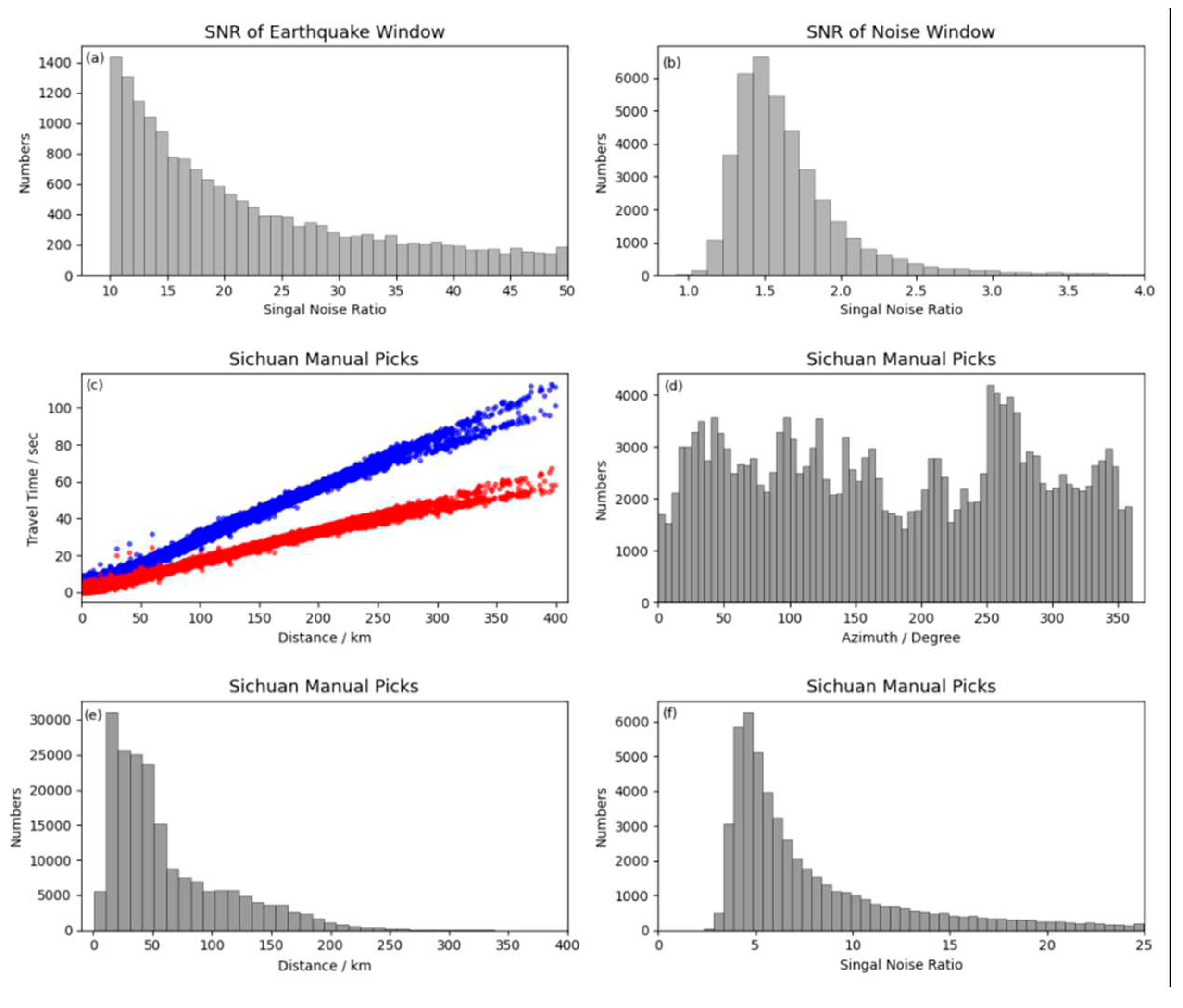
After assembling all sample sets, we conducted a thorough analysis of various attributes within the dataset. This included assessing the distribution of signal-to-noise ratios, epicentral distances, azimuths, and the relationship between travel time and epicentral distance (see Figure 2). Such an analysis is essential to understand the dataset's diversity and to ensure that the deep learning models are trained on a representative and comprehensive sample of seismic data. To provide a visual understanding of these distributions, refer to Figure 2 in the paper. This figure illustrates the range and variability of the aforementioned attributes within the dataset, offering insights into the data's complexity and the challenges it poses for AI-based seismic analysis. This comprehensive preparation and analysis of the seismic AI training dataset lay the groundwork for the effective training of deep learning models, enabling them to accurately discern between seismic events and noise and to proficiently identify seismic phases, thereby contributing to the advancement of seismic research and aftershock analysis.

3.2. Methods

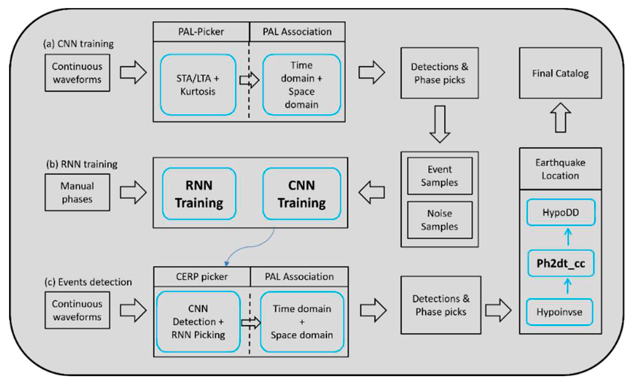
The comprehensive AI detection workflow is depicted in Figure 3. Unlike the procedural framework presented in Zhou et al. (2021)[24], the seismic phase data used in training the RNN model were manually picked by experts. In contrast, the sample dataset in Zhou et al. (2021) [24] was obtained through detection by the PAL-picker. The AI model in this study integrates a hybrid CNN & RNN structure, an approach previously developed by Zhou et al. (2019)[4]. Within this combined CNN & RNN model, the CNN deep neural network is composed of eight convolutional layers, Rectified Linear Unit (ReLU) non-linear activation functions, Max Pooling layers, and fully connected layers. The forward propagation procedure is defined by a loss function based on the L1 norm, while the backward propagation utilizes the Adam optimizer. The RNN features two bidirectional Gated Recurrent Unit (GRU) layers, which process data both forwards and backwards in time. In the RNN, each layer’s current state is influenced by both the input at the present time step and the hidden state from the preceding time step.
Phases association incorporates clustering analysis in both time and space domains[18]. Temporal association is achieved by searching for clusters of earthquake occurrence times. Spatial association is accomplished through grid searching for the hypocenter position with the minimum travel time residual. The phase association procedure ensures the detection of the same seismic signal by a minimum of four stations, thereby reducing the likelihood of misidentified signals. The magnitude estimation is determined by calculating the body wave magnitude using the S-wave amplitude. The earthquake localization utilizes Hypoinverse[25] for absolute location and HypoDD[26,27] for relative relocation (Klein, 2002; Waldhauser, 2000).

3.3. AI model training

To improve the performance of the AI model under specific tectonic and observation conditions, we rapidly constructed a sample dataset for the local region and retrained the AI model. The methodology for curating the AI training dataset has been delineated in the preceding section. Before feeding samples into the AI model, data augmentation techniques were employed on the original dataset to enhance its robustness. This included temporal adjustments of the sampling window and the infusion of varying degrees of white noise. Specifically, the P-wave arrival served as the temporal anchor around which five random shifts within a 15-second interval were executed, each accompanied by the introduction of white noise ranging from 0 to 40%.
The hyperparameters, notably the learning rate and batch size, are pivotal in the AI training process, influencing model convergence, the risk of overfitting, and computational efficiency. An inordinately high learning rate can precipitate non-convergence, while an excessively low learning rate may unduly protract the convergence timeline. Similarly, a minuscule batch size could prove inadequate in counterbalancing the stochastic influence on gradient estimation, whereas an excessively large batch size could lead to protracted iteration durations. For the training executed in this study, we utilized hardware equipped with a GeForce RTX 3090 GPU, boasting 24GB of memory. A learning rate of 0.001 was established for both CNN and RNN training, with a batch size of 512. The training dataset was apportioned into training, validation, and test sets following a 7:2:1 ratio.
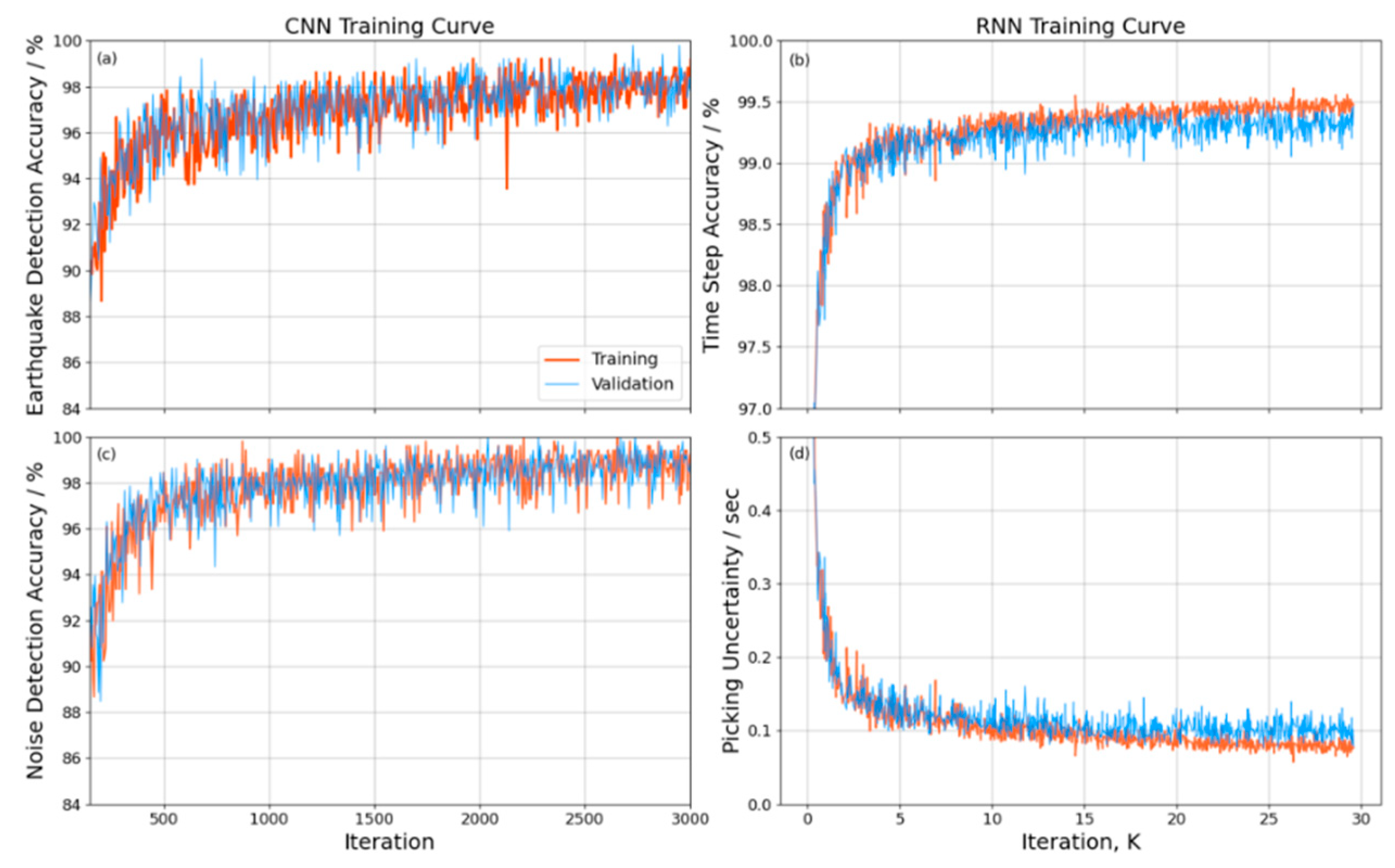
Detection accuracy was quantified as the proportion of correct predictions derived from the training dataset during the CNN training epoch, while validation accuracy was ascertained using the validation dataset. An observed increment in detection accuracy concomitant with a decrement in validation accuracy typically denotes the phenomenon of overfitting within the AI training regime. The 30-second sampling window was dissected into multiple time steps with a granularity of 0.5 second. The accuracy of these time steps, along with the validation rate, was defined as the likelihood of accurately predicting the P & S phases within these temporal increments during the RNN training phase. The picking uncertainty is characterized as the temporal precision in identifying the P & S arrivals within the training/validation datasets during the RNN training phase. The trajectories of detection/validation accuracy, picking uncertainty, and time step accuracy are graphically represented in Figure 4.

3.4. Earthquake detection, phase picking, association and location

Utilizing the retrained CNN & RNN models on continuous waveform data, we conducted earthquake detection over a 30-second window with a 15-second sliding step, applying a 1-20 Hz bandpass filter to 24-hour three-component waveforms. P & S phases were concurrently picked within this framework, and surface wave amplitudes were quantified within an amplitude window extending from 1 second pre P-wave to 5 seconds post S-wave. After obtaining the P & S phases for all stations, clustering of phase arrival times is achieved using a threshold of 2.0 seconds for grid search travel time residual, and a requirement of at least 4 stations simultaneously recording the same seismic signal. This process culminated in initial detections comprising 3624 seismic events and 25125 P & S phase arrivals. A juxtaposition of the AI-determined arrival times with those manually picked revealed an average temporal discrepancy for P-waves of 0.02 second (standard deviation of 0.32 second), and for S-waves, an average discrepancy of 0.11 second (standard deviation of 0.44 second).
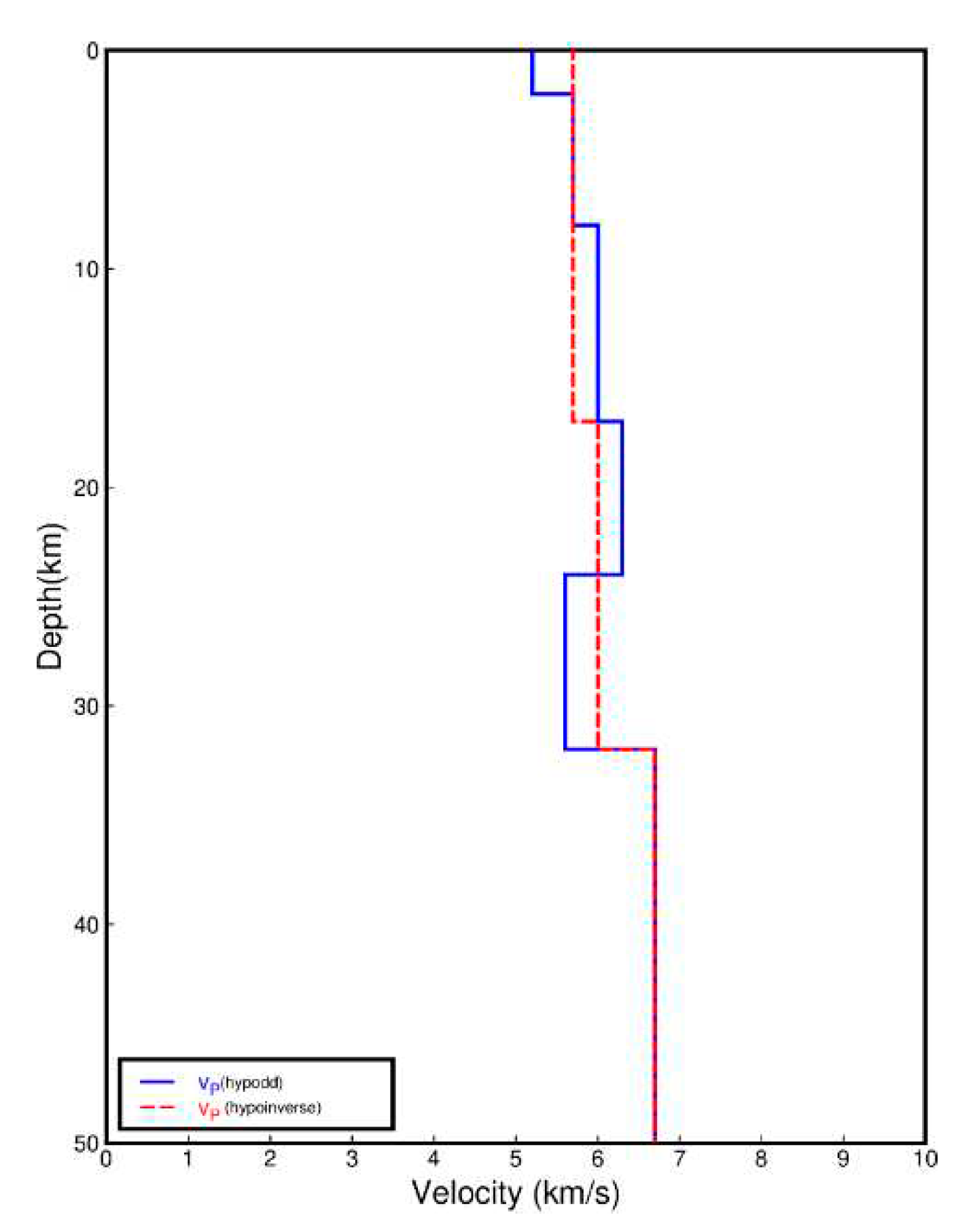
For absolute earthquake localization, the Hypoinverse software was harnessed. We adopted an average strategy for the initial velocity model, utilizing an averaged three-layer model of Fang et al (2014, Figure 5)[19]. Throughout the iterative inversion process, station weights were modulated based on the root mean square of the travel time residuals and epicentral distance. A residual cutoff threshold was established, affording full weight to stations with residuals under 0.3 second, nullifying weights for residuals exceeding three times of the cutoff residual (0.9 second), and implementing weighted interpolation for intermediate values according to a cosine function curve. A distance cutoff was set at 40 km, with a cutoff range spanning 40-120 km.
Subsequent to the absolute localization, relative localization was performed employing the HypoDD algorithm. The double-difference method incorporates an initial relative location derived from travel time measurements, further refined by cross-correlation to correct temporal disparities, thereby augmenting the precision of the relative locations. The parameters included a maximum station-event distance of 150 kilometers, an events pair distance constraint of 6 kilometers, and a minimum of 8 phases per events pair. After two cycles and eight iterations, the inversion parameters, inclusive of travel time residuals, horizontal and vertical discrepancies, were stabilized. During the cross-correlation for travel time difference calculations (cc), the maximum distance between events pairs is set to 4 kilometers, and the maximum epicentral distance for stations is 120 kilometers. Template windows are defined as P-wave before 0.5 second and after 3.5 seconds, and S-wave before 0.3 second and after 4.5 seconds, using a bandpass filter of 2-15 Hz. The velocity model is the same as the one used by Fang et al. (2014, Figure 5). Finally, we obtained high-precision location results for 3286 events.
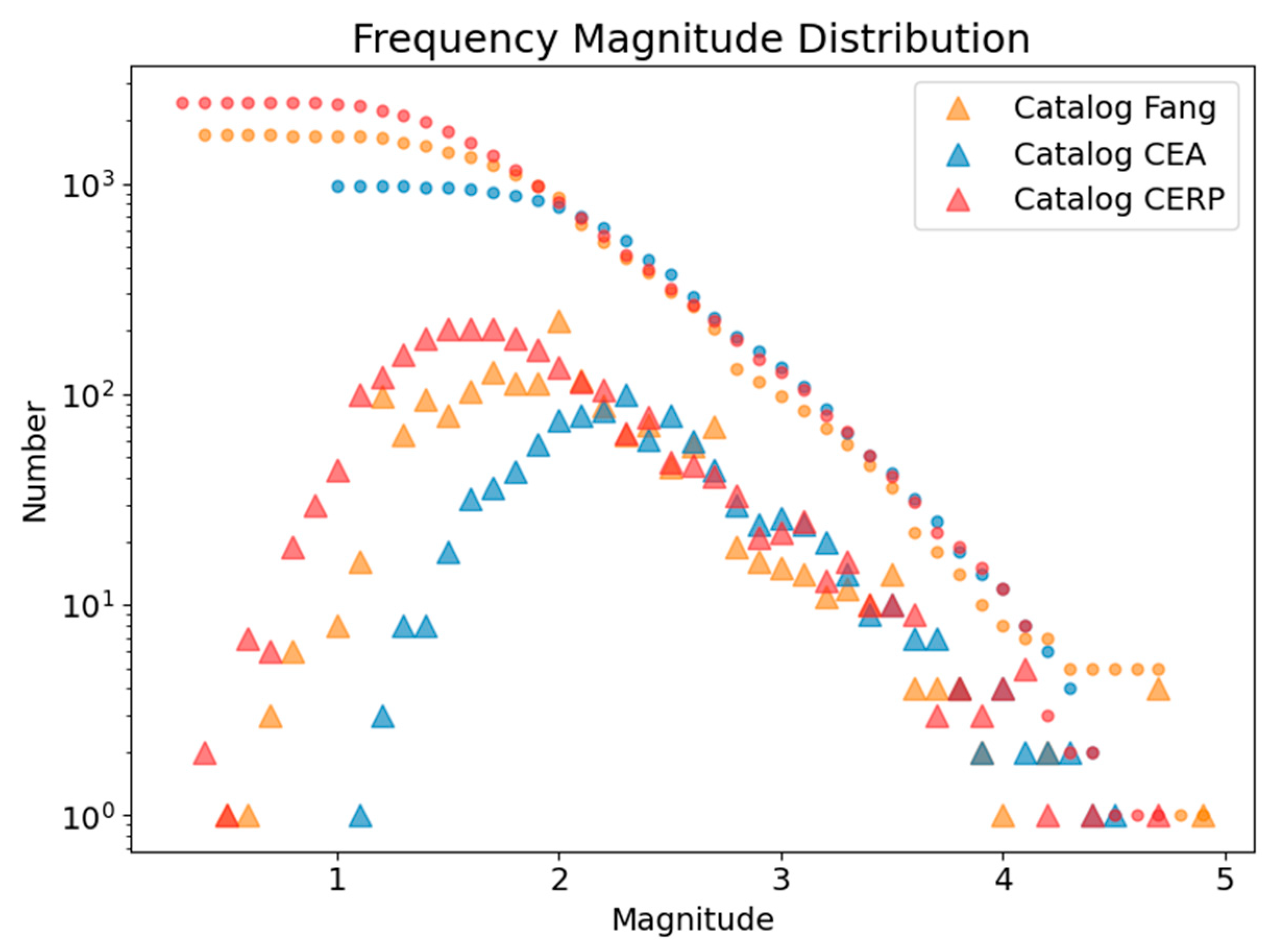
The Frequency-Magnitude Distribution (FMD) between the AI catalog of this study and those compiled by Fang et al. (2014) and the China Earthquake Network Center (CENC) was contrasted (Figure 6). This comparative analysis indicated that the AI-generated catalog exhibits superior detection capabilities relative to the catalogs by Fang et al. (2014) and CENC.

4. Results and Discussion

4.1. Aftershocks space distribution, temporal evolution and focal mechanism

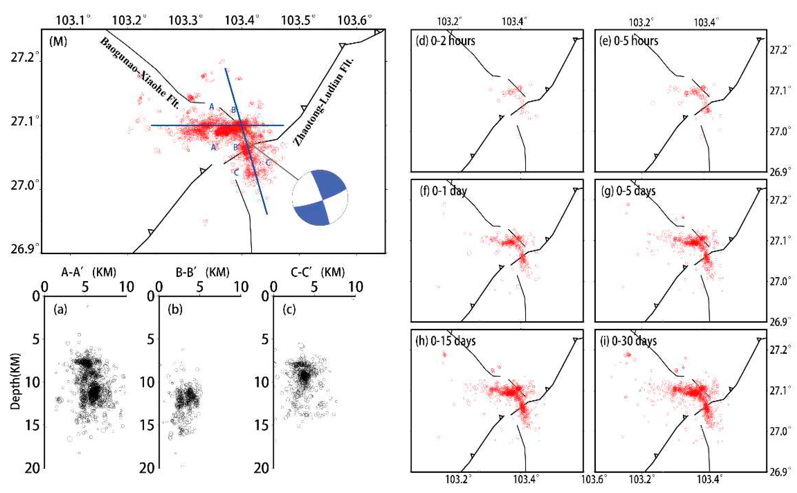
The analysis of the aftershock sequence following the 2014 Ludian Ms6.5 earthquake elucidates a distinct L-shaped conjugate distribution, suggesting a compound fracture orientation primarily along east-west (E-W) and northwest-southeast (NW-SE) axes. The E-W oriented section spans approximately 23 kilometers in length and 5 kilometers in breadth, while the NW-SE extension measures about 18 kilometers in length and similarly 5 kilometers across. In terms of depth, the aftershocks predominantly clustered within a stratum extending from 5 to 15 kilometers beneath the surface. The intersection of the conjugate faults marks the zone of maximal hypocentral depth, where the concentration of aftershocks is notably dense. Moving laterally from this central intersection, there is a discernible gradation towards more superficial seismic events (Figure 7).
The aftershocks also exhibited distinct spatiotemporal variation characteristics. Initially, within the first 2 to 5 hours post-main shock, the aftershocks predominantly aligned in a northwest-southeast (NW-SE) orientation, forming a strip-like distribution. This pattern underwent a notable shift approximately 5 hours later, with the emergence of a northeast-southwest (NE-SW) directional trend in the aftershock distribution. This NE-SW orientation became increasingly pronounced over the subsequent 24 hours. Remarkably, after five days, the aftershock sequence evolved to display an asymmetric conjugate distribution, further illustrating the dynamic nature of the seismic event's aftershock activity.
The focal mechanism solutions for the two nodal planes, as published by the Global Centroid Moment Tensor (GCMT)[28,29], were consistent with the dominant orientations of the L-shaped conjugate distribution of aftershocks. On the other hand, this spatiotemporal patterning of the Ludian aftershock sequence concurred with the observations presented in the works of Fang et al. (2014)[19] and Wang et al. (2014)[30]. The consistency of these findings across independent studies lends credence to the interpretation of the tectonic behavior in the aftermath of the Ludian earthquake and reinforces the understanding of seismic dynamics in conjugate fault systems. The deployment of AI-enhanced seismic detection and location methodologies, as described, has contributed to a more nuanced and detailed understanding of the aftershock sequence, which may have significant implications for seismic hazard analysis and tectonic research in the region.

4.2. Seismic rate evolution

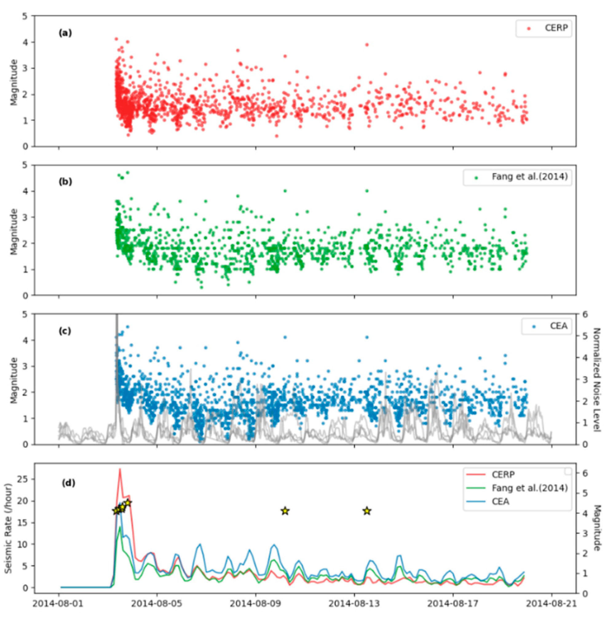
The seismic rate, defined as the frequency of earthquakes occurring per hour, peaked within the initial day following the main shock, and thereafter exhibited a general diminishing trend. This decay in seismic rate over time is a typical characteristic of aftershock sequence, as postulated by established seismic laws, such as Omori’s law for aftershock temporal decay. The observed magnitude-time relationship and seismic rate for the aftershocks also presented conspicuous diurnal patterns. These patterns were discerned to be linked to the diurnal variations in the ambient noise level, which in turn affected the earthquake detection capability of the monitoring system. During periods of heightened daily noise—such as human activity during daytime hours—the ability to detect smaller seismic events is often compromised. Conversely, the relative quietude of nighttime generally corresponds to higher detection rates of smaller aftershocks.
Furthermore, the seismic detection capability is also temporally affected by the ‘tail waves’ of larger seismic events. These trailing seismic waves generate a transient increase in the noise floor, which can substantially diminish the detection efficiency for smaller magnitude earthquakes in the period following significant aftershocks. The impact of these larger events on detection capability is visually represented in Figure 8, which likely includes a time series plot showing the variation in seismic rate alongside the occurrence of larger aftershocks. Such fluctuations in detection capability necessitate careful consideration when analyzing seismicity rates and the corresponding magnitude distributions. These variations underscore the importance of incorporating noise level assessments and potential detection biases into the seismic analysis to ensure the accurate interpretation of seismicity patterns and the underlying physical processes driving the aftershock sequence.

4.3. Seismogenic fault

Within the vicinity of epicenter, the NE-oriented Zhaotong-Ludian fault is primarily recognized for its thrust faulting. However, the focal mechanism of strike-slip and the spatial-temporal pattern of aftershocks, which align predominantly along NW-SE and near E-W directions, imply that the Zhaotong-Ludian fault may not be the only seismoginic fault. The presence of the NW-oriented Baogunao-Xiaohe fault, noted for its left-lateral strike-slip movement, provides an alternative tectonic feature that corresponds more closely with the aftershock distribution and focal mechanism. Particularly within the first 5 hours following the main shock, the predominance of aftershocks in the NW-SE direction, coupled with their depth characteristics consistent with a strike-slip fault, suggested that the Baogunao-Xiaohe Fault may have been the seismogenic fault for the Ludian earthquake. Synthesizing the aftershocks’ spatial-temporal pattern, the focal mechanism, and the intrinsic characteristics of the regional faults, we postulate that the seismogenic fault responsible for the Ludian earthquake is the NW-oriented Baogunao-Xiaohe fault.
The distribution of the NW-trending Ludian aftershocks, intersecting the NE-trending Zhaotong-Ludian fault, suggests that the former may be transecting the latter. This intersection could imply that the Zhaotong-Ludian fault, despite its longstanding geological presence, has been intersected and possibly offset by the younger Baogunao-Xiaohe fault, a tectonic feature that may have developed during the Cenozoic era[19]. Furthermore, geological structural maps indicate that the Baogunao-Xiaohe Fault is a minor and less distinct fault located north of the Zhaotong-Ludian Fault. On the south side of the Zhaotong-Ludian Fault lies another small fault, with both minor faults being separated by the Zhaotong-Ludian Fault. The distribution of aftershocks suggests that the 2014 Ludian earthquake may have interconnected the Baogunao-Xiaohe Fault across the north and south sides of the Zhaotong-Ludian Fault. The proximity of the Baogunao-Xiaohe Fault to the Zhaotong-Ludian Fault, and the presence of another small fault on the latter's southern side, suggest a complex fault system in the region. The interaction between these faults could influence seismic activities and seismic hazards in the region.

5. Conclusions

A high-resolution catalog for the 2014 Ms6.5 Ludian aftershocks is constructed based on an AI-picker model. During the AI model training process, we designed a specific training strategy, which combined the advantages of the STA/LTA algorithm and AI algorithm. Our successful retraining and detection results indicate that, this training strategy for building a sample set in a specific tectonic region to retrain the AI model can improve the generalization performance of AI model in the specific region. Compared to the previous results from the Fang et al. (2014)[19] and China Earthquake Networks Center (CENC), our result exhibits superior performance in both location accuracy and the number of aftershock events. According to the accurate distribution of aftershocks, we conclude that, (1) the seismogenic fault of Ludian earthquake is the NW-trending Baogunao-Xiaohe Fault. (2) the Ludian aftershocks interconnected the discontinuous NW-trending Baogunao-Xiaohe Fault, and intersected with the Zhaotong-Ludian Fault. (3) It suggests that the NE-trending Zhaotong-Ludian Fault may have been intersected by the NW-trending Baogunao -Xiaohe Fault, indicating that the Baogunao-Xiaohe Fault is likely a relatively young Neogene fault.

Funding

This research was funded by the Nature Science Foundation of China (NSFC) projects, grant number U2139205 and 42374104.

Acknowledgments

The authors thank Dr. Zhou Yijian and Prof. Fang Lihua for their guidance and assistance in the methods and conceptualization of this study. The authors also thank Pro. Xu Lisheng for his providing mobile seismic data in Ludian region.

Conflicts of Interest

All of authors declare no conflict of interest.

References

  1. Shelly, D.R. A High-Resolution Seismic Catalog for the Initial 2019 Ridgecrest Earthquake Sequence: Foreshocks, Aftershocks, and Faulting Complexity. Seismological Research Letters 2020, 91, 1971–1978. [Google Scholar] [CrossRef]
  2. Ross, Z.E. , Idini, B., Jia, Z., Stephenson, O.L., Zhong, M.Y., Wang, X., Zhan, Z.W., Simons, M., Fielding, E.J., Yun, S.H., Hauksson, E., Moore, A.W., Liu, Z., and Jung, J. Hierarchical interlocked orthogonal faulting in the 2019 Ridgecrest earthquake sequence. Science 2019, 366, 346–351. [Google Scholar] [CrossRef] [PubMed]
  3. Ross, Z.E. , Trugman, D.T., Hauksson, E., and Shearer, P.M. Searching for hidden earthquakes in Southern California. Science 2019, 364, 767–771. [Google Scholar] [CrossRef] [PubMed]
  4. Zhou, Y.J. , Yue, H., Kong, Q.K., and Zhou, S.Y. Hybrid Event Detection and Phase-Picking Algorithm Using Convolutional and Recurrent Neural Networks. Seismological Research Letters, 1079. [Google Scholar] [CrossRef]
  5. LeCun, Y. , Bengio, Y., and Hinton, G. Deep learning. Nature 2015, 521, 436–44. [Google Scholar] [CrossRef] [PubMed]
  6. Zhu, W.Q. and Beroza, G.C. PhaseNet: A Deep-Neural-Network-Based Seismic Arrival Time Picking Method. Geophysical Journal International 2018. [CrossRef]
  7. Mousavi, S.M., Zhu, W.Q., Sheng, Y.X., and Beroza, G.C. CRED: A Deep Residual Network of Convolutional and Recurrent Units for Earthquake Signal Detection. Scientific Reports 2019, 9. [CrossRef]
  8. Mousavi, S.M., Ellsworth, W.L., Zhu, W.Q., Chuang, L.Y., and Beroza, G.C. Earthquake transformer—an attentive deep-learning model for simultaneous earthquake detection and phase picking. Nature Communications 2020, 11. [CrossRef]
  9. Perol, T. , Gharbi, M., and Denolle, M. Convolutional neural network for earthquake detection and location. Science Advances 2018, 4, e1700578. [Google Scholar] [CrossRef] [PubMed]
  10. Ross, Z.E. , Meier, M.A., Hauksson, E., and Heaton, T.H. Generalized Seismic Phase Detection with Deep Learning. Bulletin of the Seismological Society of America 2018, 108, 2894–2901. [Google Scholar] [CrossRef]
  11. Wang, J., Xiao, Z.W., Liu, C., Zhao, D.P., and Yao, Z.X. Deep Learning for Picking Seismic Arrival Times. Journal of Geophysical Research: Solid Earth 2019, 124, 6612-6624.
  12. Park, Y., Mousavi, S.M., Zhu, W.Q., Ellsworth, W.L., and Beroza, G.C. Machine-Learning-Based Analysis of the Guy-Greenbrier, Arkansas Earthquakes: A Tale of Two Sequences. Geophysical Research Letters 2020, 47.
  13. Liu, M., Zhang, M., Zhu, W.Q., Ellsworth, W.L., and Li, H.Y. Rapid Characterization of the July 2019 Ridgecrest, California, Earthquake Sequence From Raw Seismic Data Using Machine-Learning Phase Picker. Geophysical Research Letters 2020, 47.
  14. Zhao, M., Xiao, Z.W., Chen, S., and Fang, L.H. DiTing: A large-scale Chinese seismic benchmark dataset for artificial intelligence in seismology. Earthquake Science 2022, 35, 1-11. [CrossRef]
  15. Mousavi, S.M., Sheng, Y.X., Zhu, W.Q., and Beroza, G.C. STanford EArthquake Dataset (STEAD): A Global Data Set of Seismic Signals for AI. IEEE Access 2019, 7, 179464-179476. [CrossRef]
  16. Jiang, C. , Fang, L.H., Fan, L.P., and Li, B.R. Comparison of the earthquake detection abilities of PhaseNet and EQTransformer with the Yangbi and Maduo earthquakes. Earthquake Science 2021, 34, 425–435. [Google Scholar] [CrossRef]
  17. Allen, R.V. Automatic earthquake recognition and timing from single traces. Bulletin of the seismological society of America 1978, 68, 1521–1532. [Google Scholar] [CrossRef]
  18. Zhou, Y.J., Yue, H., Fang, L.H., Zhou, S.Y., Zhao, L., and Ghosh, A. An Earthquake Detection and Location Architecture for Continuous Seismograms: Phase Picking, Association, Location, and Matched Filter (PALM). Seismological Research Letters 2021, 93, 413-425. [CrossRef]
  19. Fang, L.H., Wu, J.P., Wang, W.L., Lv, Z.Y., Wang, C.Z., Yang, T., and Zhong, S.J. Relocation of the aftershock sequence of the M S 6.5 Ludian earthquake and its seismogenic structure. Seismology and Geology 2014, 36(4): 1173-1185.
  20. Wen, X.Z., Du, F., Yi, G.X., Long, F., Fan, J., Yang, F.X., Xiong, R.W., Liu, Q.X., and Liu, Q. Earthquake potential of the Zhaotong and Lianfeng fault zones of the eastern Sichuan-Yunnan border region. Chinese Journal of Geophysics 2013, 56(10):3361-3372.
  21. He, H.L., Ikeda, Y., He, Y.L., Togo, M., Chen, J., Chen, C.Y., Tajikara, M., Echigo, T., and Okada, S. Newly-generated Daliangshan fault zone — Shortcutting on the central section of Xianshuihe-Xiaojiang fault system. Science in China Series D: Earth Sciences 2008, 51, 1248-1258. [CrossRef]
  22. Xu, X.W., Wen, X.Z., Zheng, R.Z., Ma, W.T., Song, F.M., and Yu, G.H. Pattern of latest tectonic motion and its dynamics for active blocks in Sichuan-Yunnan region, China. Science in China Series D Earth Sciences 2003, 46, 210-226. [CrossRef]
  23. Baillard, C., Crawford, W.C., Ballu, V., Hibert, C., and Mangeney, A. An Automatic Kurtosis-Based P- and S-Phase Picker Designed for Local Seismic Networks. Bulletin of the Seismological Society of America 2013, 104, 394-409. [CrossRef]
  24. Zhou, Y.Y., Ghosh, A., Fang, L.H., Yue, H., Zhou, S.Y., and Su, Y.J. A high-resolution seismic catalog for the 2021 MS6.4/MW6.1 Yangbi earthquake sequence, Yunnan, China: Application of AI picker and matched filter. Earthquake Science 2021, 34, 390-398. [CrossRef]
  25. Klein, F.W., User's Guide to HYPOINVERSE-2000, a Fortran Program to Solve for Earthquake Locations and Magnitudes, in Open-File Report. 2002.
  26. Waldhauser, F. and Ellsworth, W. A double-difference earthquake location algorithm: Method and application to the northern Hayward fault, California. Bulletin of the seismological society of America 2000, 90, 1353-1368.
  27. Waldhauser, F. and Ellsworth, W.L. Fault structure and mechanics of the Hayward Fault, California, from double-difference earthquake locations. Journal of Geophysical Research: Solid Earth 2002, 107.
  28. Dziewonski, A.M., Chou, T.A., and Woodhouse, J.H. Determination of earthquake source parameters from waveform data for studies of global and regional seismicity. Journal of Geophysical Research: Solid Earth 1981, 86, 2825-2852. [CrossRef]
  29. Ekström, G., Nettles, M., and Dziewoński, A.M. The global CMT project 2004–2010: Centroid-moment tensors for 13,017 earthquakes. Physics of the Earth and Planetary Interiors 2012, 200-201, 1-9.
  30. Wang, W., Wu, J., Fang, L., and Juan, L. Double difference location of the Ludian MS6.5 earthquake sequences in Yunnan province in 2014. Chinese Journal of Geophysics (in Chinese) 2014, 57, 3042-3051.
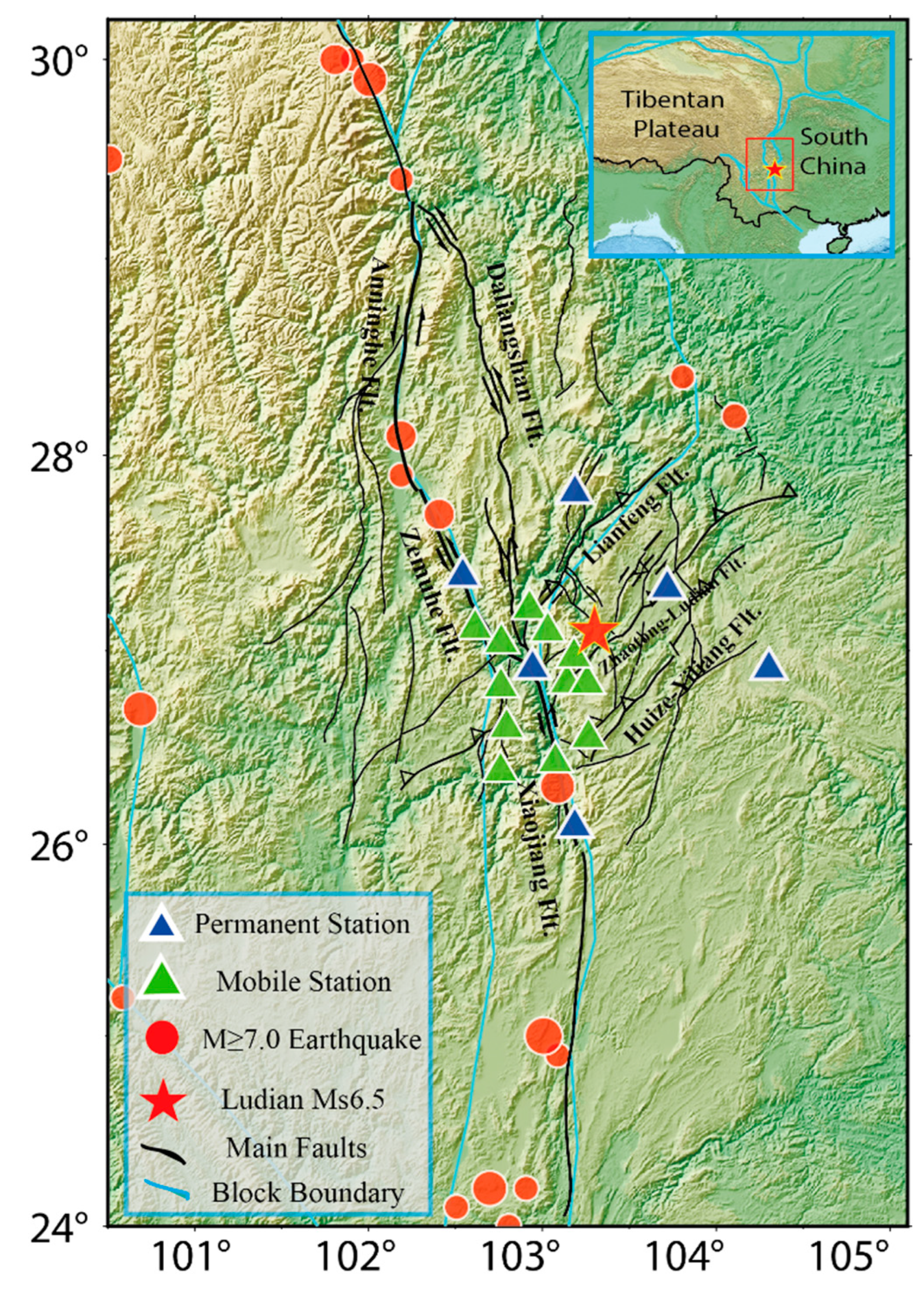
Figure 1. The tectonic background, seismic station distribution and historical large earthquakes in study area. Blue triangles and green triangles represent the permanent stations and campaign stations, respectively. The red circles represent the historical earthquakes greater than 7.0. The red star represents the 2014 Ms6.5 Ludian earthquake. The black solid curves represent the primary active faults, and the blue solid curves represent the block boundary in China mainland.
Preprints 93171 g001
Figure 2. Histograms of signal-to-noise ratio, epicentral distance, azimuth, and travel time-to-epicentral distance relationship in the training dataset. (a) and (b) depict the distribution of signal-to-noise ratio for earthquake and noise samples in the CNN training set. (c), (d), (e), and (f) represent histograms of the travel time-to-epicentral distance relationship, azimuth, epicentral distance, and signal-to-noise ratio in the RNN training set.
Preprints 93171 g002
Figure 3. The workflow of earthquake detection and location. The blue boxes represent important processing steps, while the black boxes indicate input and output data.
Preprints 93171 g003
Figure 4. Detection accuracy and picking uncertainty over the course of CNN & RNN training iterations. (a) and (c) represent the training accuracy and validation accuracy respectively for event samples and noise samples during the iteration process of the CNN model. Here, the red curve denotes the training accuracy, while the blue curve represents the validation accuracy. (b) and (d) correspond to the time step accuracy and picking uncertainty respectively during the iteration process of the RNN model, where the red curve indicates the accuracy on the training set, and the blue curve signifies the accuracy on the validation set.
Preprints 93171 g004
Figure 5. The velocity model used in Ludian region. The red dashed line represents the averaged P-wave velocity from Fang et al.,2014[19], which is used for absolute localization with HypoInverse, while the blue solid line indicates the P-wave velocity model from Fang et al.,2014[19], used for relative localization with HypoDD.
Preprints 93171 g005
Figure 6. Comparison of frequency magnitude distribution. The solid circles and solid triangles represent the cumulative and non-cumulative distribution, respectively. These indicate the relationship between the number of earthquakes equal to or greater than a certain magnitude. The red symbols represent the CERP catalog in this study, orange symbols represent the earthquake catalog by Fang et al. 2014[19], and blue symbols represent the earthquake catalog from the China Earthquake Administration’s station network, which overlap with the fixed stations used in this study.
Preprints 93171 g006
Figure 7. The space distribution and temporal evolution of the Ludian aftershocks. (M) shows the spatial horizontal distribution of the Ludian aftershocks, while (a), (b), and (c) represent the depth of aftershocks along three profiles showed in (M). Insert figures (d-i) illustrate the temporal evolution of aftershocks within 30 days after the main shock. The focal mechanism is from the Global Centroid Moment Tensor Project (https://www.globalcmt.org/)[28,29].
Preprints 93171 g007
Figure 8. Seismicity-time distribution of the Ludian aftershock catalog. (a), (b), (c) represent the earthquake catalogs obtained in this study (CERP), the earthquake catalog by Fang Lihua et al. (2014), and the earthquake catalog from the China Earthquake Administration regional seismic network, respectively. Panel (d) shows the seismicity rate calculated from the three earthquake catalogs between August 1, 2014, and August 21, 2014. The seismicity rate is defined as the number of earthquakes occurring per hour in the region.
Preprints 93171 g008
Disclaimer/Publisher’s Note: The statements, opinions and data contained in all publications are solely those of the individual author(s) and contributor(s) and not of MDPI and/or the editor(s). MDPI and/or the editor(s) disclaim responsibility for any injury to people or property resulting from any ideas, methods, instructions or products referred to in the content.
Copyright: This open access article is published under a Creative Commons CC BY 4.0 license, which permit the free download, distribution, and reuse, provided that the author and preprint are cited in any reuse.
Prerpints.org logo

Preprints.org is a free preprint server supported by MDPI in Basel, Switzerland.

Subscribe

© 2024 MDPI (Basel, Switzerland) unless otherwise stated