Enhancing Credit Card Fraud Detection: An Ensemble Machine Learning Approach

In the era of digital advancements, the escalation of credit card fraud necessitates the development of robust and efficient fraud detection systems. This paper delves into the application of machine learning models, specifically focusing on ensemble methods, to enhance credit card fraud detection. Through an extensive review of existing literature, we identified limitations in current fraud detection technologies, including issues like data imbalance, concept drift, false positives/negatives, limited generalisability, and challenges in real-time processing. To address some of these shortcomings, we propose a novel ensemble model that integrates a Support Vector Machine (SVM), K-Nearest Neighbor (KNN), Random Forest (RF), Bagging, and Boosting classifiers. This ensemble model tackles the dataset imbalance problem associated with most credit card datasets by implementing under-sampling and the Synthetic Over-sampling Technique (SMOTE) on some machine learning algorithms. The evaluation of the model utilises a dataset comprising transaction records from European credit card holders, providing a realistic scenario for assessment. The methodology of the proposed model encompasses data pre-processing, feature engineering, model selection, and evaluation, with Google Colab computational capabilities facilitating efficient model training and testing. Comparative analysis between the proposed ensemble model, traditional machine learning methods, and individual classifiers reveals the superior performance of the ensemble in mitigating challenges associated with credit card fraud detection. Across accuracy, precision, recall, and F1-score metrics, the ensemble outperforms existing models. This paper underscores the efficacy of ensemble methods as a valuable tool in the battle against fraudulent transactions. The findings presented lay the groundwork for future advancements in the development of more resilient and adaptive fraud detection systems, crucial as credit card fraud techniques continue to evolve.

Keywords:

Subject: Computer Science and Mathematics - Artificial Intelligence and Machine Learning

1. Introduction

Identity theft fraud has the potential to result in substantial financial losses and adversity for its victims. According to the National Crime Agency (NCA), identity theft fraud is characterised by the act of impersonating someone else and exploiting their personal information for fraudulent purposes. This form of deception empowers criminals to pilfer money and inflict harm upon unsuspecting victims. The surge in digital transactions and online activities has heightened the risk of identity theft fraud, underscoring the need for robust safeguards against this pervasive criminal activity [1].

Credit card fraud stands out as a prominent manifestation of identity theft fraud, drawing significant attention owing to its pervasive nature and adverse financial implications. The Federal Trade Commission (FTC) report underscores the severity of the issue, noting that 2021 marked the most challenging year in history for identity theft. As depicted in Figure 1, credit card fraud emerges as the predominant form of identity theft fraud [2]. It is crucial to note that many cases of identity theft go unreported, suggesting that the actual number may surpass the reported figures. The FTC report emphasises the need for innovative approaches to safeguard the financial well-being of both consumers and businesses.

Various approaches, including Statistical, Machine Learning, and Deep Learning methods, are utilised for credit card fraud detection. Statistical techniques such as Regression, hypothesis testing, and clustering are applied to identify and analyse anomalies in credit card transactions. In contrast, machine learning methods leverage algorithms to detect fraudulent activity in real time by analysing historical data. Deep learning methodologies utilise neural networks to autonomously identify intricate patterns and features within complex datasets, resulting in exceptionally accurate detection of fraudulent activities.

Within the realm of machine learning for credit card fraud detection, ensemble methods have gained popularity. These methods combine predictions from individual base models to create a model that is robust and accurate. Techniques like Bagging, boosting, and stacking have proven effective in handling imbalanced datasets and reducing the occurrence of false positives and false negatives. This paper aims to analyse and evaluate the effectiveness of ensemble strategies in credit card fraud detection, contributing to the advancement of an efficient and reliable fraud prevention system.

The main contributions of this paper are as follows:

To propose an effective credit card fraud detection model that addresses the challenge of imbalanced datasets, where fraud occurrences are uncommon in comparison to genuine transactions.
To compare the performance of various machine learning models in identifying credit card fraud, such as Support Vector Machine (SVM), K-Nearest Neighbor (KNN), Random Forest (RF), Bagging, and Boosting.
To benchmark the performance of the proposed model with existing credit card fraud detection models.

The remainder of the paper is organised as follows. Section 2 reviews the related works that have been done to detect credit card fraud using different ML and DL techniques. Section 3 of the paper introduces the proposed model architecture and methodology.

2. Related work

In this section, we examine the related literature on proposed systems and techniques for credit card fraud detection. The existing work in this field is categorised into three sections based on the technique used, i.e. Statistical methods, Machine Learning Algorithms and Deep Learning Techniques.

2.1. Statistical Methods

Statistical approaches have been extensively employed in the identification of credit card fraud. These methods discover suspicious trends by analysing the statistical properties of transaction data [3]. Statistical models identify outlier transactions using thresholds or criteria. Popular statistical methods include Descriptive Statistics, Hypothesis Testing and Time-Series Analysis.

Descriptive statistics, hypothesis testing, and time-series analysis detect credit card fraud. Descriptive statistics, such as mean, standard deviation, and percentiles, can help uncover abnormal transactions [4]. Hypothesis testing compares genuine and fraudulent transactions using null and alternative hypotheses and statistical tests like t-tests or chi-square tests [5]. ARIMA (AutoRegressive Integrated Moving Average) models and STL (Seasonal and Trend Decomposition using Loess) provide transaction data patterns and trends for fraud detection [6].

2.2. Deep Learning (DL) in Credit Card Fraud Detection

Deep learning teaches multi-layered neural networks hierarchical data representations. These techniques collect complex patterns and relevant attributes from high-dimensional data. They revolutionised computer vision, natural language processing, and credit card fraud detection. Convolutional Neural Networks (CNN), Long Short-Term Memory (LSTM), Multilayer Feed Forward Neural Networks (MLFF), Artificial Neural Networks (ANNs) and Recurrent Neural Networks (RNNs) are some of the deep learning algorithms.

Deep learning techniques, such as Convolutional Neural Networks (CNN), Long Short-Term Memory (LSTM), and Generative Adversarial Networks (GAN), have revolutionised various fields, including credit card fraud detection. CNNs are adept at classifying images and extracting features from temporal data, making them suitable for detecting fraud in transaction sequences. LSTM, as a recurrent neural network, excels at analysing sequential data and capturing long-term dependencies, allowing it to identify complex fraud patterns involving multiple transactions effectively. GANs, with their generator and discriminator networks, can synthesise realistic fraud patterns, enhancing the adaptability and robustness of fraud detection systems. These deep-learning approaches have significantly improved the accuracy and efficiency of credit card fraud detection [12,13,14,15].

2.3. Machine Learning (ML) in Credit Card Fraud Detection

Due to the ability to learn from data, find complex patterns, and predict credit card theft, machine learning algorithms are important in credit card fraud detection. These algorithms are supervised and unsupervised learning methods. A few of the algorithms used for CCFD (Credit Card Fraud Detection) include Logistic Regression (LR), Support Vector Machines (SVM), K-Nearest Neighbors (KNN), Naive Bayes (NB), Decision Trees (DT), Random Forest (RF) and Tree-Augmented Naive Bayes (TAN).

For credit card fraud detection, SVM, KNN, NB, DT, RF, and TAN are powerful machine learning models. SVM classifies data points using the best hyperplane [7], KNN classifies transactions based on their K-Nearest Neighbors [8], NB uses probabilistic learning to estimate class probabilities [9], DT generates decision trees for feature-based classification [9], RF combines decision trees to reduce overfitting [10], and TAN enhances NB with a tree-like dependency structure to capture feature correlations [11]. These models offer diverse approaches to identifying and preventing fraudulent transactions, contributing to robust fraud detection systems. Credit card fraud detection algorithms have pros and downsides. When choosing an algorithm for an application, consider dataset size, feature space, processing needs, interpretability, and fraud.

Several researchers have highlighted the route to improved fraud prevention and detection in this comprehensive analysis of credit card fraud detection with machine learning. In [16], Prasad Chowdary et al. propose an ensemble technique to improve credit card fraud detection. The authors focus on optimising model parameters, improving performance measures, and integrating deep learning to fix identification errors and reduce false negatives. Decision Tree (DT), Gradient Boosting Classifier (XGBoost), Logistic Regression (LR), Random Forest (RF), and Support Vector Machine were used in this paper. The paper compares these algorithms across multiple evaluation metrics and finds that DT performs best with a 100% recall value, followed by XGBoost, LR, RF, and SVM with 85%, 74.49%, 75.9%, and 69%, respectively. By combining multiple classifier ensembles and rigorously assessing their performance, this project greatly improves CCFD system efficiency. However, the evaluation parameters reveal the low performance of the model.

Sahithi, Roshmi et al., in [17], developed a credit card fraud detection algorithm in 2022. This model uses a Weighted Average Ensemble to combine Logistic Regression (LR), Random Forest (RF), K-Nearest Neighbors (KNN), Adaboost, and Bagging. The paper used the European Credit Card Company dataset. Their model had 99% accuracy, topping base models like RF Bagging (98.91%), LR (98.90%), Adaboost (97.91%), KNN (97.81%), and Bagging (95.37%). This paper shows that their ensemble model can detect credit card theft in this key domain. Nevertheless, the feature selection process was not provided, which hinders reproducibility.

Also, in 2022, Qaddoura and Biltawi [18] investigated the effectiveness of oversampling methods: SMOTE, ADASYN, borderline1, borderline2, and SVM oversampling algorithms for credit card fraud detection. The paper used Random Forest (RF), Logistic Regression (LR), Naive Bayes (NB), K-Nearest Neighbor (KNN), Support Vector Machine (SVM), and Decision Tree. The authors found that oversampling can improve model performance, although the exact strategy depends on the machine learning algorithm. However, the applicability of the model in real-life situations can be affected due to the computational overhead.

Tanouz et al. [19] extensively studied machine learning for credit card fraud classification. The Decision Trees classifier, Random Forest (RF), Logistic Regression (LR), and Naive Bayes (NB) were evaluated, with a focus on imbalanced datasets. This investigation showed that the Random Forest (RF) approach performed well, scoring 96.77%. Logistic Regression (LR), Naive Bayes (NB), and Decision Trees classifiers had accuracy scores of 95.16, 95.16, and 91.12%, respectively. The detailed investigation shows that Random Forest is effective at credit card fraud detection, which is vital to financial security. Nonetheless, the performance of the proposed models is hampered due to the lack of feature selection.

The fundamental objective of the study in [20] undertaken by Ruttala Sailusha and colleagues was to provide a comparative examination of the Random Forest and AdaBoost algorithms in the context of credit card fraud detection. The findings of their analysis demonstrated similar levels of accuracy when comparing the two algorithms. It is worth mentioning that the Random Forest method demonstrated higher performance in terms of precision, recall, and F1-score when compared to Adaboost. However, the dataset used by the authors is skewed, with no clear mention of how the issue was addressed.

The primary objective of the research performed by Sadgali, Sael, and Benabbou [21] was to identify the most effective approaches for detecting financial fraud. The methodology employed in their paper involved the utilisation of a wide range of techniques, such as Support Vector Machine (SVM), Bayesian Belief Networks, Naive Bayes, Genetic Algorithm, Multilayer Feed Forward Neural Network (MLFF), and Classification and Regression Tree (CART). Significantly, as a comprehensive and evaluative investigation of previous scholarly studies, the present paper did not necessitate the use of a particular dataset for analysis. The presented results highlight the dominant performance of Naive Bayes, which achieved the greatest accuracy rate of 99.02%. SVM closely followed it with an accuracy rate of 98.8% and Genetic Algorithm with an accuracy rate of 95%. Despite that, the authors limit their work to insurance fraud.

The study conducted by Raghavan and El Gayar [22] aimed to detect anomalies or fraudulent actions using data mining techniques. They utilised three distinct datasets from Australia (AU), Germany, and the European (EU) to achieve this objective. Their work employed Support Vector Machine (SVM), K Nearest Neighbor (KNN), and Random Forest algorithms, in addition to creating two separate ensembles: one integrating KNN, SVM, and Convolutional Neural Network (CNN) and another combining KNN, SVM, and Random Forest. The findings highlight the dominant performance of the Support Vector Machine (SVM) in terms of accuracy, achieving a notable rate of 68.57%. In comparison, Random Forest and KNN exhibited accuracies of 64.37% and 60.47% respectively. The present paper offers a comprehensive examination that yields useful information regarding the effectiveness of various algorithms and ensemble tactics within the domain of fraud detection. However, the performance of the model was low for all the datasets used.

Saputra and Suharjito [23] compare the effectiveness of Decision Tree, Naïve Bayes, Random Forest, and Neural Network machine learning approaches. SMOTE was used to solve the problems of imbalanced datasets. Kaggle provided this study's dataset. At 0.093% of records, the dataset included few fraudulent transactions. The examination using confusion matrices revealed that the Neural Network had the highest accuracy (96%), followed by Random Forest (95%), Naïve Bayes (95%), and Decision Tree (91%). SMOTE enhanced the average F1-Score and G-Score performance measures and addressed skewed data, proving its benefits. However, the dataset used in the paper does not fully represent all the e-commerce platforms.

A comparative analysis of credit card fraud detection methods was conducted by Tiwari et al. [24]. The authors examined SVM, ANN, Bayesian Network, K-Nearest Neighbor (KNN), Hidden Markov Model, Fuzzy Logic-Based System, and Decision Trees. Analysis of the KDD dataset from the standard KDD CUP 99 Intrusion Dataset showed differing accuracy levels across approaches. SVM had 94.65% accuracy, ANN 99.71%, Bayesian 97.52%, K-Nearest Neighbors 97.15%, Hidden Markov Model (HMM) 95.2%, Fuzzy Logic-Based System 97.93%, and Decision Trees 94.7%. This extensive assessment sheds light on numerous credit card fraud detection methods. However, the dataset does not fully depict financial activities.

Naik and Kanikar [25] evaluate and compare some machine learning algorithms, including Naïve Bayes, J48, Logistic Regression, and AdaBoost, in the domain of Credit Card Fraud Detection (CCFD). Their approach utilises an online dataset consisting of 1000 items that contain both fraudulent and non-fraudulent transactions. The results indicate high levels of accuracy, with Logistic Regression and AdaBoost having a perfect accuracy rate of 100%. Naïve Bayes and J48 also display noteworthy accuracies of 83% and 69.93%, respectively. The findings above highlight the diverse skills of different algorithms in tackling the complexities associated with credit card fraud detection situations, providing useful insights for the advancement of resilient fraud detection systems. Nevertheless, the dataset used by the authors was limited to 1000 credit card transaction records, which is not typical of the credit card user population. Table 1 presents a summary of ensemble machine learning models used for credit card fraud detection.

3. Methodology

Machine learning detects fraud by leveraging historical data on both fraudulent and non-fraudulent transactions. ML algorithms excel at identifying abnormalities in transactions before they escalate into unmanageable issues. Figure 1 illustrates the flow diagram depicting how machine learning detects credit card fraud.

As shown in Figure 1, the initial step in the process involves selecting a dataset containing records of both legitimate and fraudulent transactions. Due to the presence of unordered, raw, missing, or duplicate instances in the dataset, system predictions may be prone to inaccuracies, necessitating data pre-processing. To address data imbalance, the sampling of imbalanced datasets is performed. Subsequently, the organised and sampled data is divided into Training and Testing samples, where the chosen machine learning models are trained using the Training sample, and both samples are employed to observe the behaviour of the trained models. Following the acquisition of results for selected evaluation parameters such as accuracy, precision, recall, confusion matrix, and AU-ROC values, performance is analysed and compared. The methodology employed in this paper adopts an experimental design, aiming to create and execute a practical experiment for credit card fraud detection.

3.1. Dataset

For our model training and testing, the Credit Card Fraud Detection dataset [29] is utilised. The dataset contains records of transactions conducted by European credit cardholders over a span of two days. In the dataset, there are 492 instances of fraud out of a total of 284,807 transactions during the specified time frame. Notably, the dataset exhibits significant skewness, with the positive class (frauds) representing only 0.172% of all transactions. Each transaction in the dataset is associated with 28 additional features labelled as V1-V28. Due to confidentiality concerns, these features have been transformed using Principal Component Analysis (PCA). It is important to note that the 'Time' and 'Amount' features are exceptions to this transformation; PCA has not altered them. The 'Time' feature represents the elapsed time in seconds between each transaction and the first transaction in the dataset. On the other hand, the 'Amount' feature corresponds to the transaction amount [29].

3.2. The Proposed Model

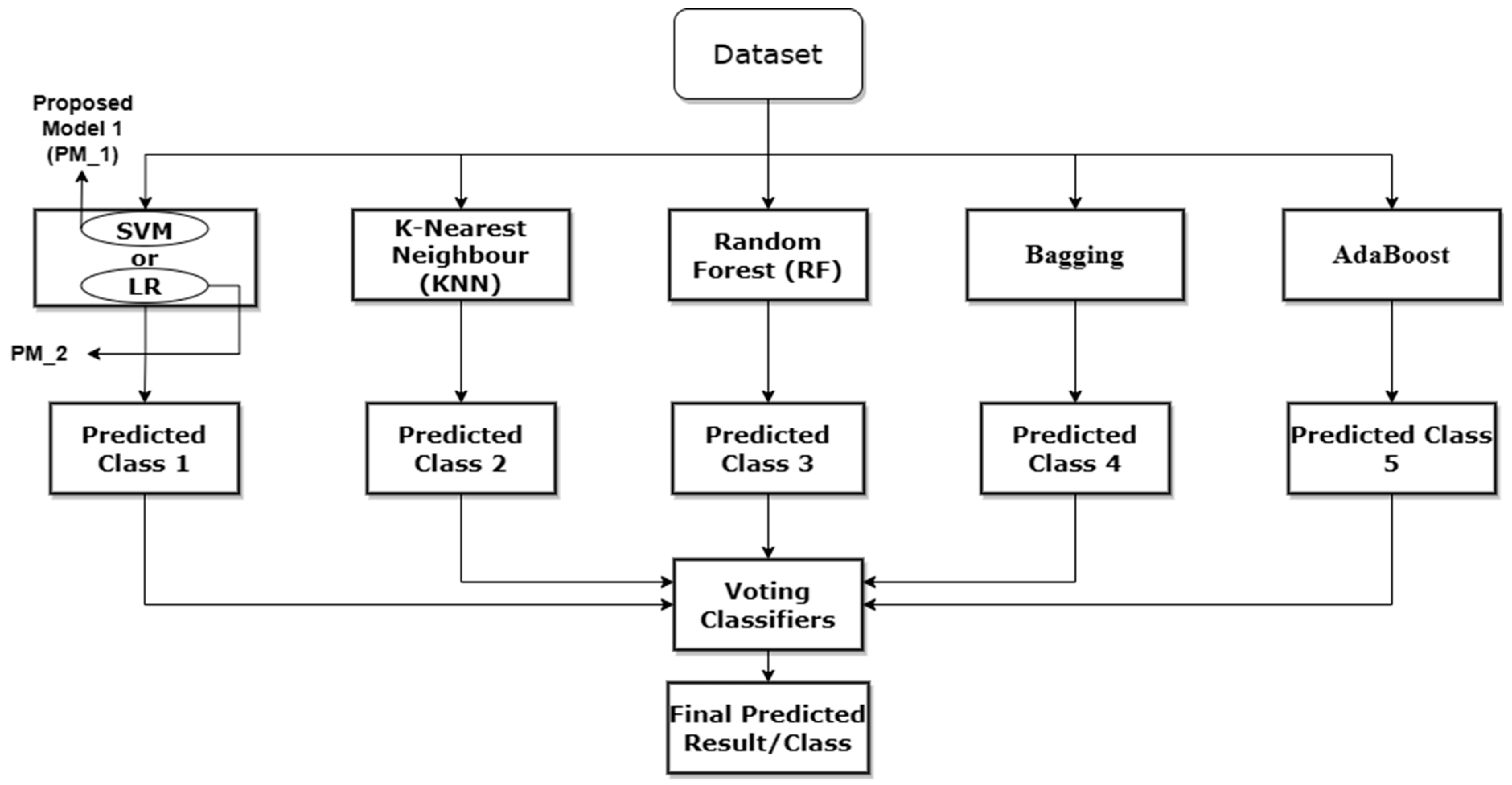
The proposed model for this paper is displayed in Figure 2. The experimental approach, contents, and architecture have been designed using insights and findings from the existing literature. This ensures that the experiment is relevant and appropriate for investigating the real-world occurrence of credit card fraud.

The experimental design of our proposed model is selected to test and assess fraud detection strategies in a controlled environment. This approach allows for variable manipulation and cause-and-effect analysis, which is vital for assessing ensemble credit card fraud detection solutions. The work uses a practical experiment to reconcile theoretical concepts and real-world applications, providing insights for constructing a strong and efficient fraud prevention system.

3.3. Hardware and Platforms

The experimental setup is supported by hardware and cloud resources. The local computer is outfitted with an Intel(R) Core (TM) i5-2520M CPU running at 2.50GHz and 12 GB of RAM, ensuring efficient processing and memory for the tasks at hand. The storage capacity of the local machine is sufficient for hosting the dataset and project files, with an extra 900 GB of cloud-based storage readily available when needed. The work primarily takes place in a cloud environment equipped with 12.68 GB of RAM and approximately 107.72 GB of disk space. These cloud-based resources significantly enhance the computational power necessary for tasks such as data processing, model creation, and training.

The selection of platforms and tools for our proposed model is guided by considerations such as usability, compatibility with chosen machine learning techniques, and the availability of pre-trained models. Notably, the well-established machine learning framework, sci-kit-learn, is employed. In terms of data pre-processing, feature extraction, and exploratory data analysis, the proposed model leverages the efficiency of pandas, NumPy, and Matplotlib. Together, these libraries provide robust capabilities for data manipulation and analysis, streamlining tasks related to data processing and exploration. For model creation and training, Google Colab is utilised, a cloud-based platform recognised for its flexibility and resource efficiency, particularly when compared to conventional platforms like Jupyter Notebook. The cloud-based architecture of Google Colab facilitates convenient access to computational resources. A comprehensive set of metrics is employed to evaluate machine learning models, encompassing accuracy, precision, recall, F1-score, confusion metrics, ROC Curve, and AU-ROC Score. To enhance data understanding and assess model performance, visualisation packages such as Matplotlib and Seaborn are employed. These libraries aid in constructing graphical representations that provide insights into data trends, model performance, and the significance of dataset aspects.

3.4. Model Design

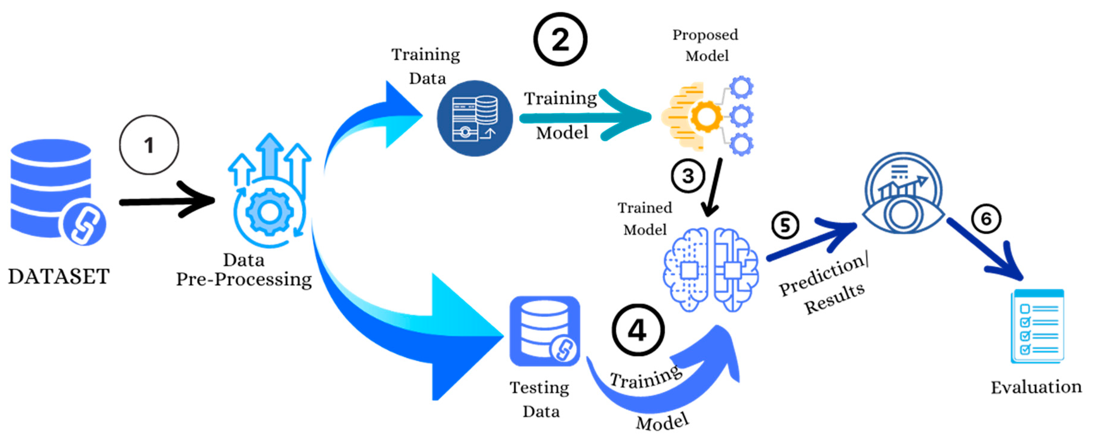
Figure 3 displays the architecture of the implementation process, encompassing dataset pre-processing and the division of the dataset into training and testing data. The training dataset is subsequently input into the chosen models for both the training and testing phases. Following this, the evaluation and results are conducted on the trained model to assess its performance.

Table 2 presents the algorithm of the proposed model. The algorithm follows a systematic approach, starting with data loading, preprocessing, and sampling. It then iterates over different machine learning model types, trains each model, and evaluates their performance using testing data. Finally, the results, including confusion matrices, are displayed for analysis.

3.4.1. Data Pre-processing

After selecting the dataset, the first step is to pre-process the data to make it suitable for model training and testing. In this step, the data was processed in the following ways.

Finding and filling/removing any null values.
Standardising the "Amount" column to make it easy for analysis.
Removing the 'Time' Column from the dataset as it was not contributing much during training and evaluation.
Checking and removing duplicate entries in the dataset.

The reason for standardising the "Amount" column instead of normalising is that, as mentioned in the description of the dataset, all features are the result of Principal Component Analysis (PCA) except 'Time' and 'Amount', and the Amount scale differs significantly from all other features (V1-V28). Hence, the 'Amount' feature is standardised.

3.4.2. Data Sampling

Following pre-processing, the subsequent step in the process involves addressing the data imbalance issue through data sampling. After pre-processing, the dataset comprises 275,190 legitimate entries and 473 fraud-labeled entries, indicating a significant skewness for model training. This paper employs two sampling techniques: under-sampling and SMOTE. The sampling process involves two steps, outlined as follows:

Separate data entries based on labels (Legit/Fraud in this case)
Apply the required sampling technique to specific data
Concatenate all data to have all data in a single dataset

3.4.2.1. Under-Sampling

In sampling, a random sample is picked from the major class, which are legit transactions (labelled as 0) in this case. The amount of random sample is determined according to the ratio required with respect to the minority class. In this paper, for better model training, the entries for both classes are made equal by choosing random sample equals to minority class entries and concatenating both classes data to have one dataset.

3.4.2.2. SMOTE (Synthetic Minority Over-Sampling Technique)

SMOTE is a statistical method for extending the number of minority class instances in a balanced manner in a dataset. The component creates new instances from existing minority cases that are provided as input [33]. So, for SMOTE, the fraud class (labelled as 1) is oversampled equal to the legit class to have identical entries for each class to train models optimally. And like under-sampling, both classes are merged to have one dataset.

3.4.3. Model Training

After the sampling process, the subsequent step involves splitting the data into training and testing samples. The training samples are utilised for model training and result assessment, while the testing samples are employed to evaluate how the model performs on unseen data. Before the data split, the "Class" column, containing the label of each entry, was separated. The dataset was then divided into training (80% of the dataset) and testing samples (20% of the dataset). Following this, the training sample is employed for model training. Once the models are trained, evaluations are conducted on both the training and testing samples, with the results discussed in the next section.

4. Results and Discussion

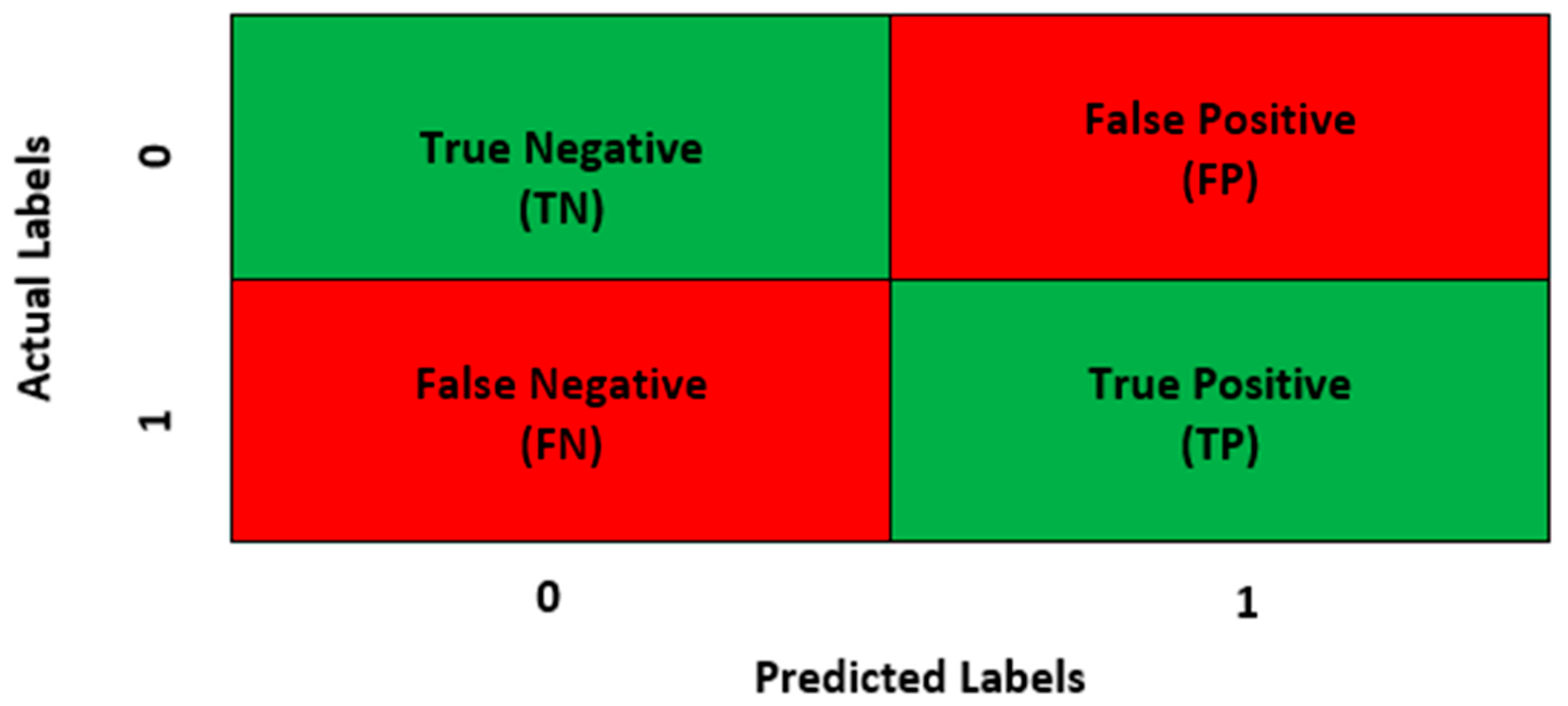
This section delves into a comprehensive discussion and analysis of the performance parameters acquired during the evaluation. It includes detailed insights into how each model performed in the context of credit card fraud detection. Prior to this discussion, the following details about the performance parameters used in this research are provided. All parameters are calculated using the True Positive (TP), True Negative (TN), False Positive (FP), and False Negative (FN) values of each model, with the confusion matrix (CM) encapsulating these values. Figure 4 visually presents a representation of the confusion matrix utilised for the proposed model, enhancing clarity and understanding.

Accuracy (ACC) is the ratio of all correct predictions (TP+TN) to the total number of predictions or entries in the sample (TP+TN+FN+FP) [34]. Equations (1 - 4) show the mathematical representation of how the Accuracy, Precision, Recall and Fi-score of a model are calculated.

Accuracy = \frac{T N + T P}{T N + F P + T P + F N}

(1)

Precision is the ratio of TP to all positive predictions (TP+FP) made by a model. In other words, it's the accuracy of the positive predictions made by the model.

Precision = \frac{T P}{T P + F P}

(2)

Recall is a metric used to measure the ability of the machine learning model to identify all relevant instances of the positive class [35]. It's the ratio of correctly predicted positive observations to the total actual positive observations.

Recall = \frac{T P}{T P + F N}

(3)

F1-score is a metric used to combine the results of precision and recall into a single value. The formula of the F1-score is as follows.

F 1 - Score = 2 \times \frac{\Pr e c i s i o n \times Re c a l l}{\Pr e c i s i o n + Re c a l l}

(4)

4.1. Performance Evaluation

The performance evaluation for both Under-sampling and SMOTE samples for each model are divulged in the sections below.

4.1.1. Under-Sampling Results

The results of the confusion matrix obtained during the evaluation of each model for under-sampling are presented in Table 3.

Based on the provided results, both RF and boosting models exhibit 0 false positive and false negative values, indicating accurate predictions for both classes. Following them, the second proposed model predicted all negative class values accurately but misclassified 20 positive class values. The proposed model with SVM (P_M_1) ranks third, with 24 false predictions for positive class values. However, relying solely on these results, derived from the data sample used for model training, is insufficient, as the models are already familiar with these data points. To assess how the models respond to unseen data, the evaluation was conducted on a testing sample of under-sampled data. Additionally, examining results on the prediction sample helps ensure that machine learning models are optimally trained, avoiding underfitting or overfitting. Table 4 displays the values of the confusion matrix for all models obtained from the Testing Sample.

The comparison of results between Table 3 and Table 4 indicates that the models are optimally fitted, as the obtained results from both samples are approximately consistent (further clarified in the discussion of other parameters). According to these findings, the second proposed model with LR (P_M_2) and bagging outperformed all other models, with ten values predicted falsely (8 FP, 2 FN). As mentioned earlier, accuracy is the ratio of all correct predictions to the total number of predictions or entries in the sample [34]. Table 5 shows the accuracy values of all models on the training sample and testing sample.

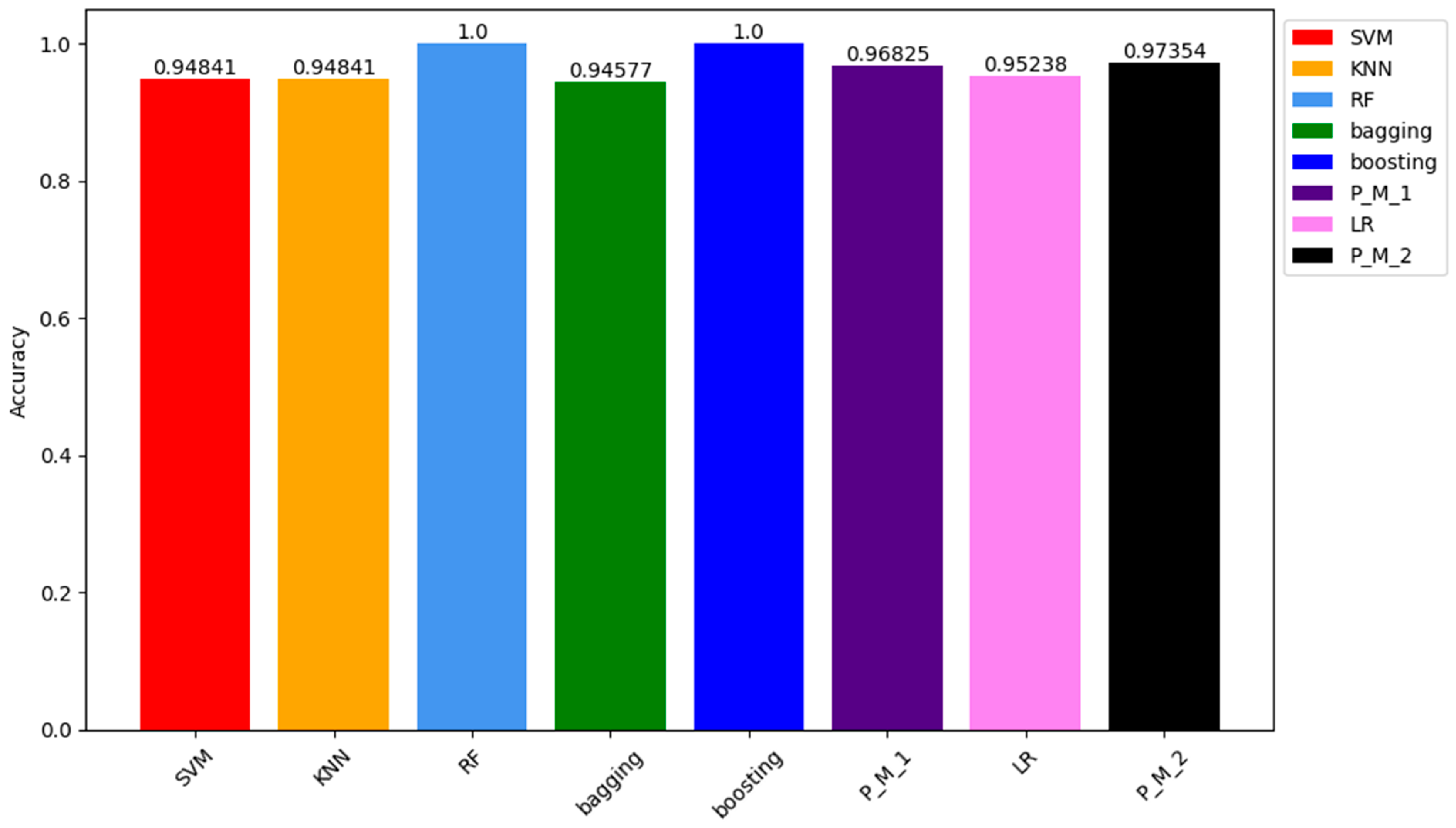
Similar to the results from the confusion matrix on training samples, the ACC of RF and Boosting models is 100%. The ACC of other models, including P_M_1, P_M_2, LR, SVM, KNN, and bagging, are 97.35%, 96.82%, 95.23%, 94.81%, 94.81%, and 94.57%, respectively. Figure 5 visually represents these values through a bar chart. Each colour in the chart corresponds to a model, with details about the colour and corresponding model specified in the legend box located at the top right corner.

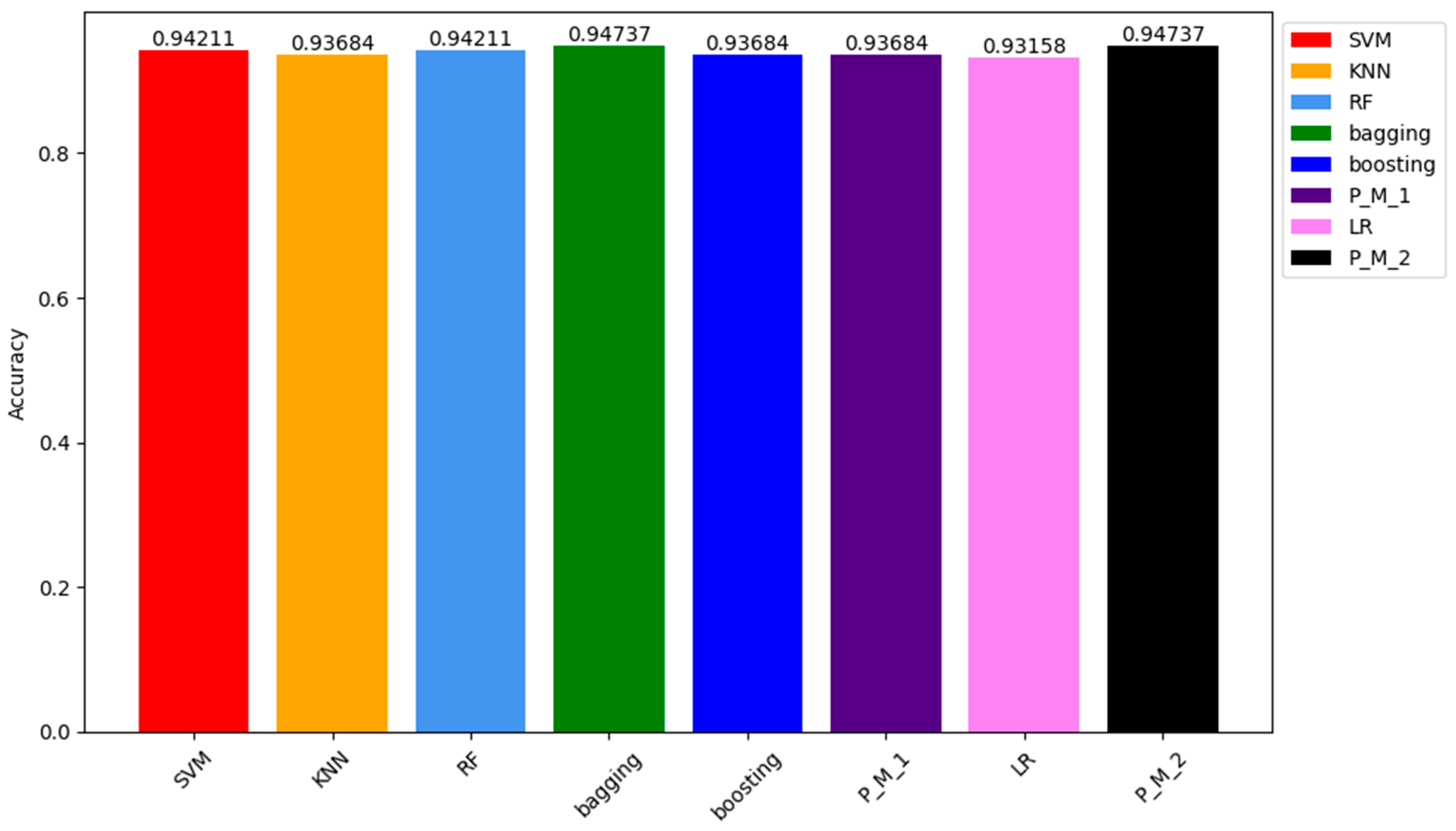
In the results obtained from the testing sample, the ACC of P_M_2 and the bagging classifier stand out as the highest among all models, reaching 94.73%. Following closely are the ACC values of SVM and RF classifiers, both at 94.21%. The ACC of KNN, Boosting, P_M_1, and LR classifiers are 93.68%, 93.68%, 93.68%, and 93.0%, respectively. The graphical representation of these results can be seen in Figure 6, which depicts how models respond to the unseen data.

The precision, recall, and F1-score of a machine learning model explain how well a classifier performs, rather than just relying on overall accuracy [35]. The results of these parameters obtained on the training sample are listed in Table 6.

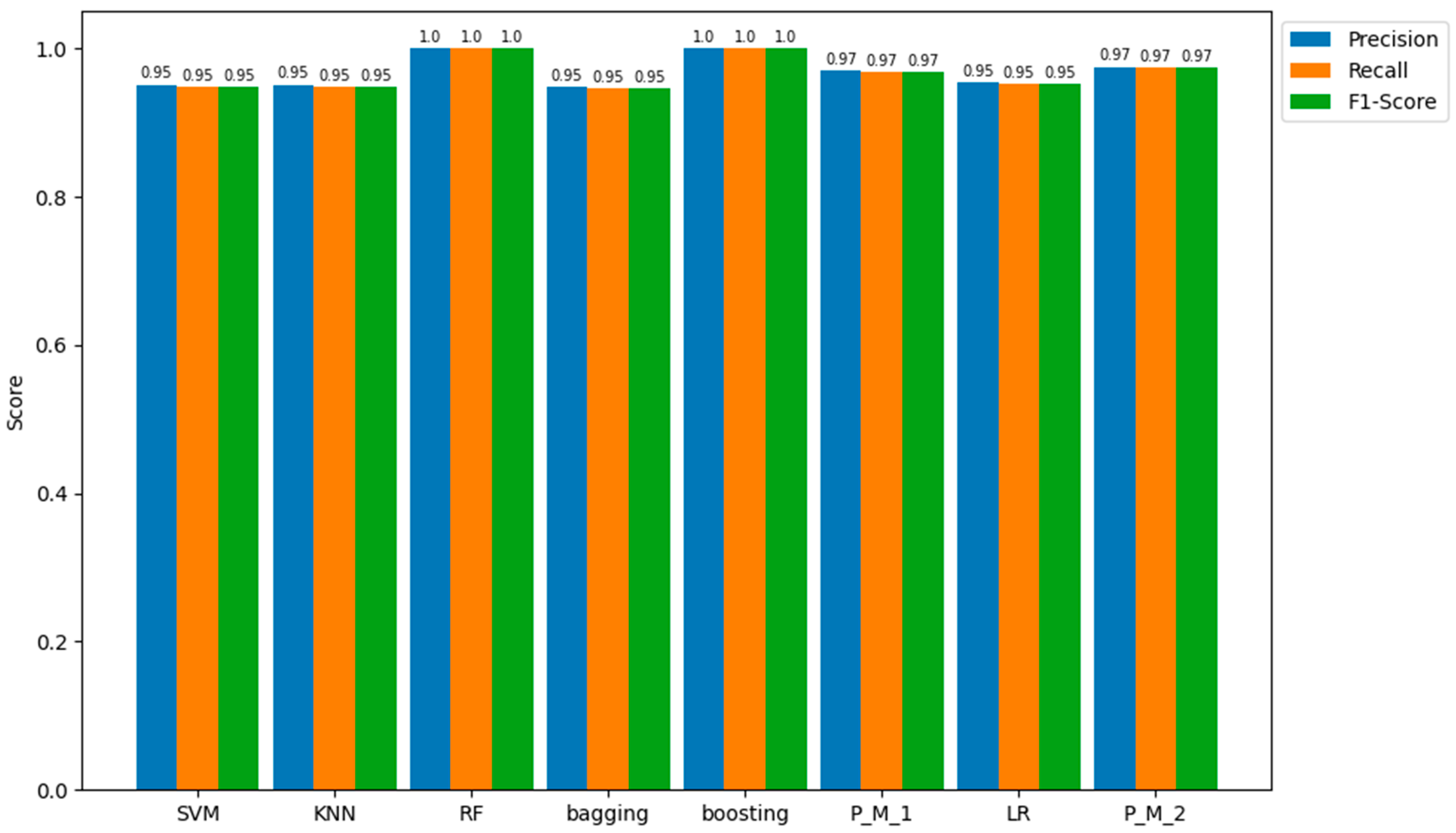
In line with the confusion matrix and ACC values, the RF and boosting classifiers demonstrated 100% precision (accuracy of positive prediction) and 100% recall (ability to identify the positive class correctly). Next to the best performing classifiers are P_M_2 and P_M_1, both achieving an accuracy of 97%. Subsequently, SVM, KNN, bagging, and LR each attain results of 95%. The representation of these parameters is visually presented in Figure 7.

Likewise, Table 7 presents the results for precision, recall, and F1-score for all models when applied to unseen samples of the under-sampled data.

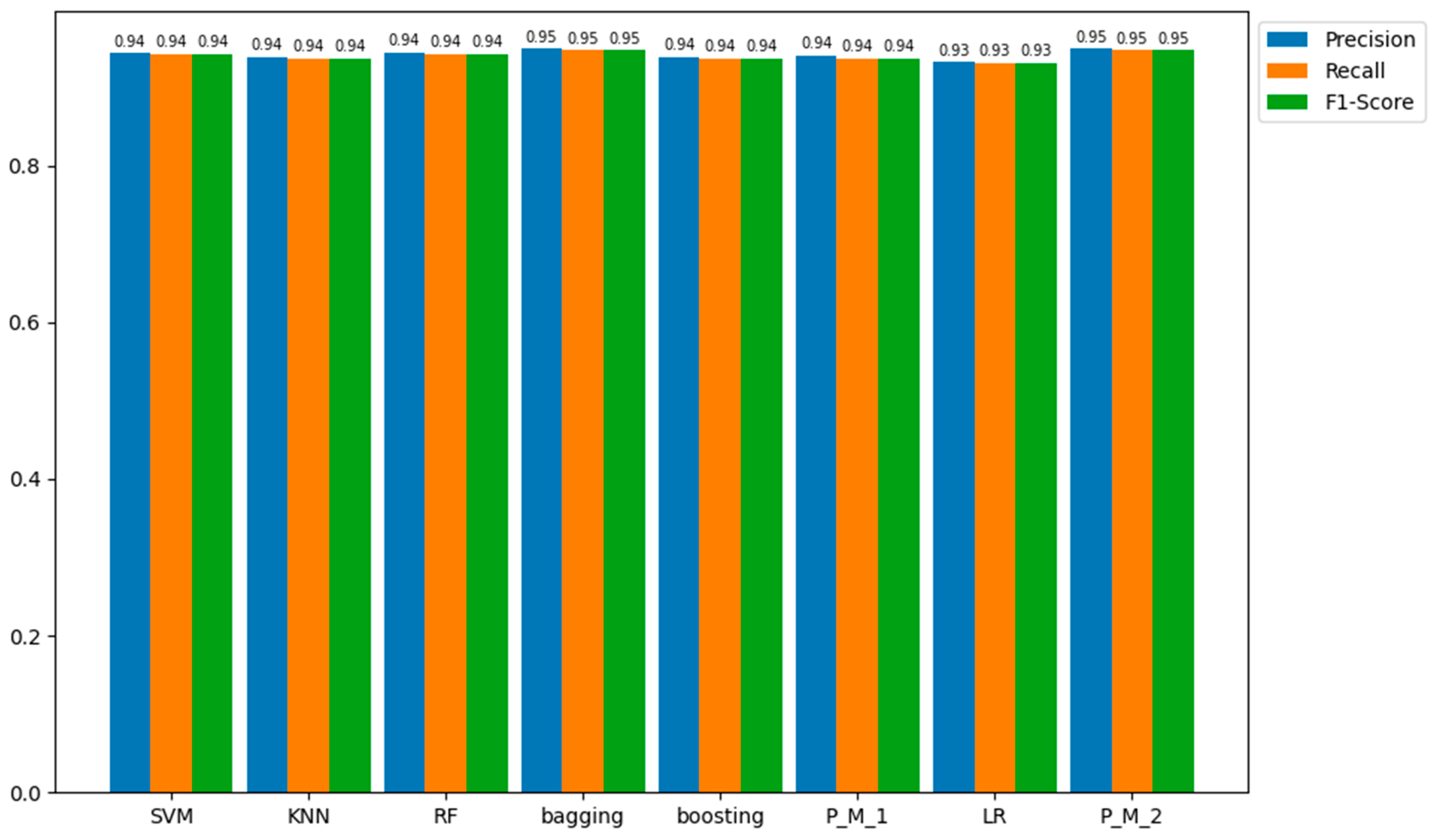
Regarding the outcomes from the testing samples, the proposed model with LR (P_M_2) emerges as the most proficient among all models in predicting the positive class (fraud), achieving precision, recall, and an F1-score of 95%. In comparison, the other models—bagging, SVM, KNN, RF, boosting, P_M_1, and LR—display precision, recall, and F1-score values of 95.0%, 94.0%, 94.0%, 94.0%, 94.0%, 94.0%, 94.0%, and 94.0%, respectively. These quantitative values are represented in Figure 8 for a more detailed understanding of these results.

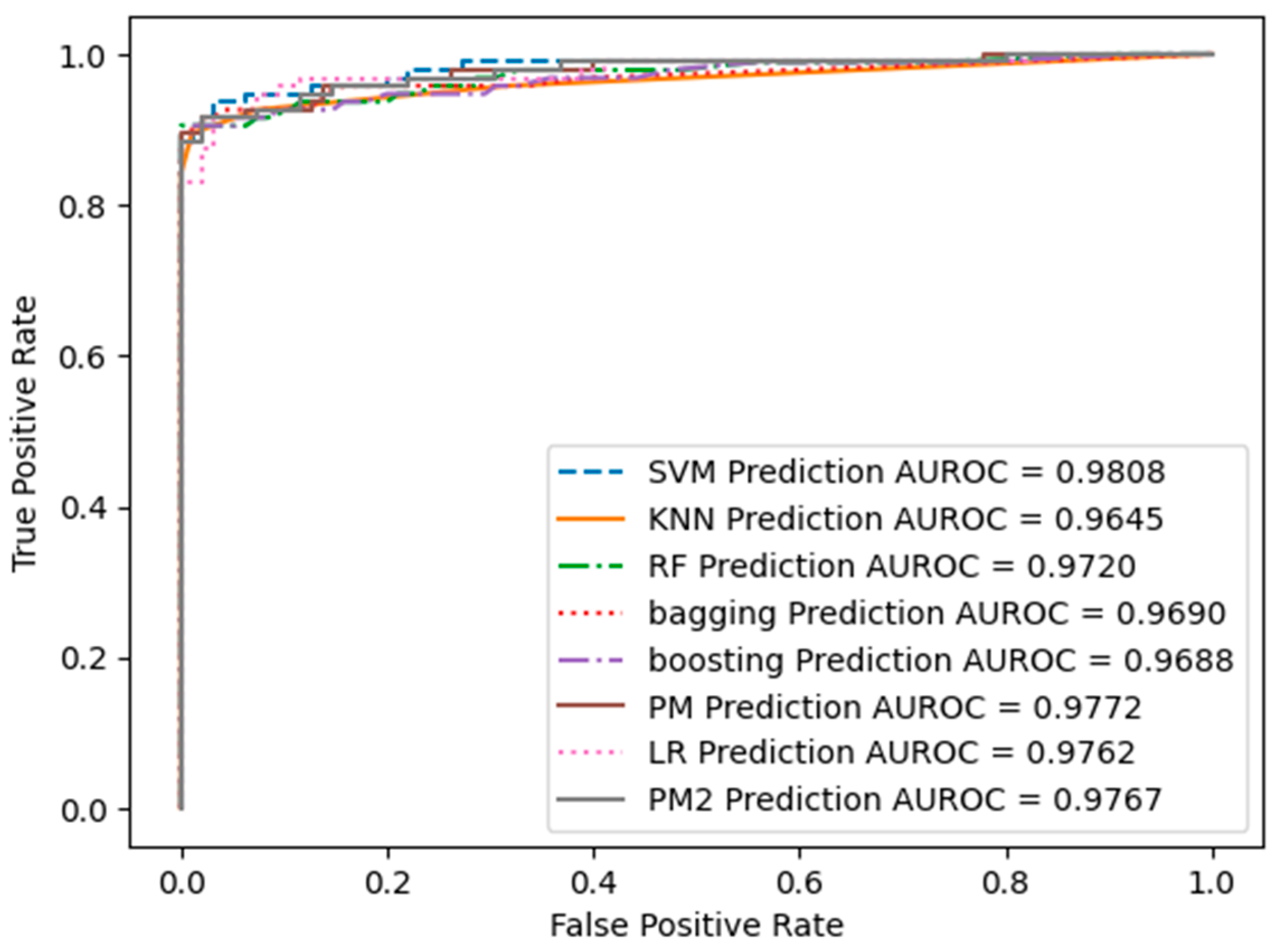
The ROC curve presented in Figure 9 illustrates the trade-off between the true positive rate (sensitivity or recall) and the false positive rate as the classifier's decision threshold varies. The ROC curve is generated by plotting the true positive rate (TPR) on the y-axis against the false positive rate (FPR) on the x-axis at different classification thresholds. Figure 9 displays the ROC curve for all models, with the corresponding AUC-ROC values of each model indicated in the bottom right corner of the image.

The ROC curves highlight distinct trade-offs between sensitivity and specificity across our models. AUC-ROC values provide a concise overview of the overall ability of the model to distinguish between positive and negative examples, with larger values indicating superior performance. Notably, the Support Vector Machine (SVM) model exhibits the highest Area Under the Receiver Operating Characteristic Curve (AUC-ROC) value at 0.9808, signifying robust discriminatory capabilities. Furthermore, the Logistic Regression (LR) model and our proposed models (P_M_1 and P_M_2) emerge as strong contenders, boasting AUC-ROC values surpassing 0.975.

4.1.2. SMOTE Results

All the training and testing results presented in this section are obtained using the SMOTE sampled dataset. Similar to the previous section, we begin by discussing the results of the confusion matrix for all models, as other parameters are derived from TP, FP, TN, and FN values, and the confusion matrix encompasses all of these values. Table 8 shows the confusion matrix for all models obtained on the oversampled dataset training sample. These confusion matrices represent the results of predictions for 440,304 entries or values present in the training sample.

The results indicate that similar to the under-sampled dataset, RF and Boosting classifiers emerge as the top-performing models, making no false predictions on the trained sample. The proposed model follows closely, exhibiting 70 false negative values and no false positive values. Subsequently, KNN and Bagging show 284 and 288 false negative values, respectively, with no false positives. LR ranks last, displaying the highest false negative and false positive values. Table 9 shows the prediction of models on the unseen sample (Testing sample).

According to the results obtained from the testing sample of 110076 entries, which were unknown entries to machine learning models, RF and boosting show the same results with 10 FN values and no FP, which are the best results compared to other models. The proposed model is second with 45 FN and 0 FP prediction, then comes KNN and bagging classifiers with 91 and 97 FN and 0 FP predictions, respectively. LR again shows the highest FN and FP results. To see the evaluation of these models in detail, other performance parameters results are discussed in the next sections. To see how accurately all models predict the Training and Testing sample. Table 11 summarises the accuracy prediction results of all the models.

Table 10. Accuracy Results of all Models on Training Sample of SMOTE Dataset.

Training Sample of SMOTE Dataset
	LR	KNN	RF	Bagging	Boosting	PM
Accuracy	0.94443	0.999354	1	0.9993	1	0.99983
Testing Sample of SMOTE Dataset
Accuracy	0.944256	0.999173	0.99989	0.999	0.999092	0.9996

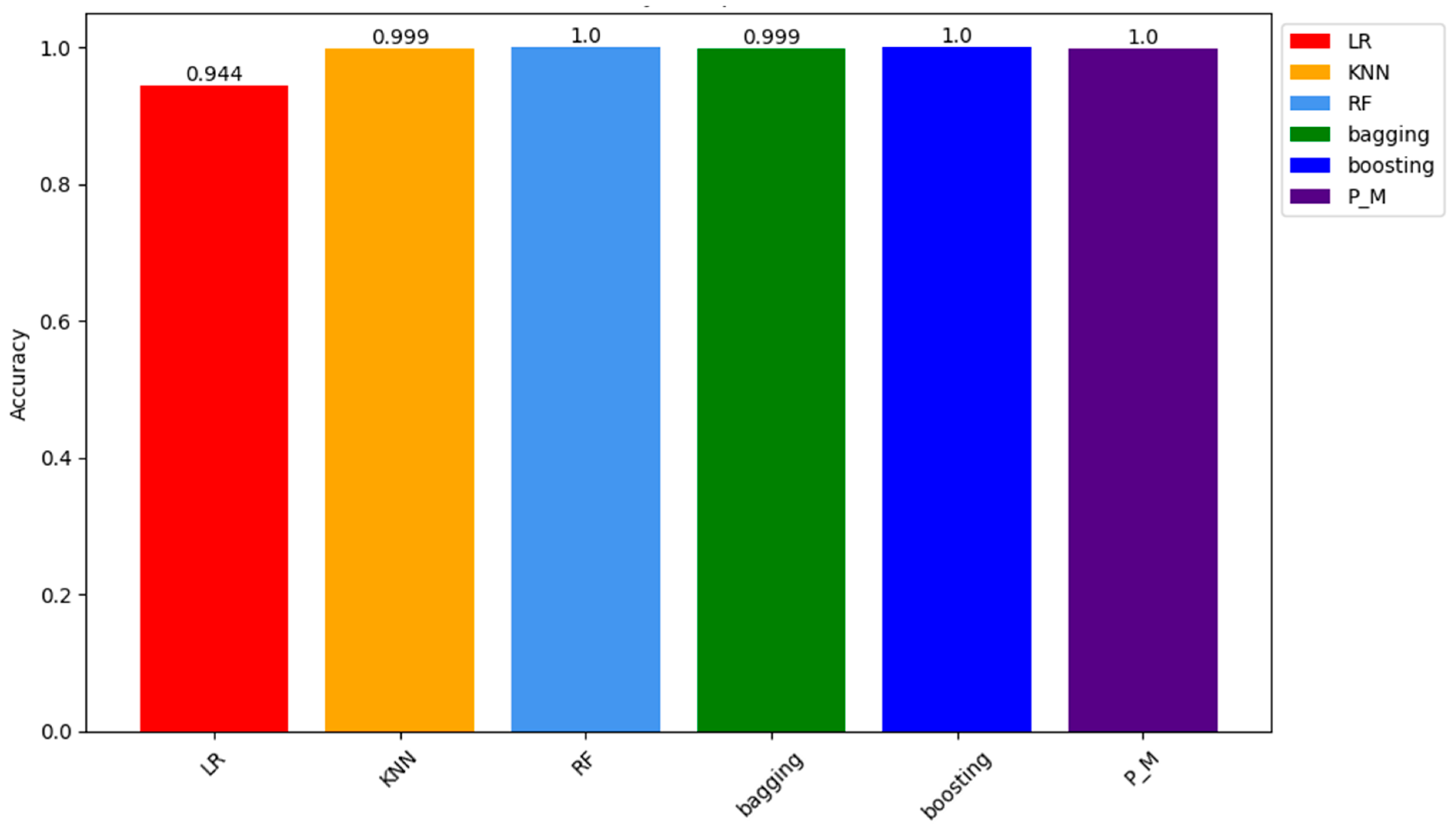
Concerning the training samples PM (Proposed Model) results, Adaboost and RF show about 100% accuracy on the seen or training sample while KNN and Bagging classifiers with 99.93% and LR is at the last with lowest accuracy of 94.44%. Figure 10 visualises the comparison results of all the models.

To see how proposed models respond to new data, the accuracy results of all models on the testing sample are also recorded in Table 10. Results on the unseen data show that significantly, the proposed models (PM) alongside Adaboost and Random Forest (RF) classifiers demonstrate remarkable accuracy, with all three converging at roughly 100% on the testing samples. This outcome highlights the effectiveness of these models in comprehending the underlying patterns present in the training data, resulting in predictions that nearly correspond to the accurate labels. Equally noteworthy, the K-Nearest Neighbors (KNN) and Bagging classifiers have a remarkable accuracy rate of 99.93%. These results are also presented visually in Figure 11.

This visual representation of the outcomes underscores the adeptness of models in extracting valuable insights from the provided training data. In contrast, Logistic Regression (LR) demonstrates a lower accuracy rate of 94.44%, indicating a relatively higher rate of misclassification compared to other models. Given the consistent presence of these patterns throughout the training sample, it reaffirms the stability and generalizability of our proposed model.

Table 11 consolidates the results of our analysis, specifically focusing on the evaluation metrics of precision, recall, and F1-score. This comprehensive depiction sheds light on the models' performance in accurately predicting the positive class within the training sample, elucidating their proficiency in correctly assessing positive class predictions (recall) and the equilibrium between these two metrics as reflected in the F1-score.

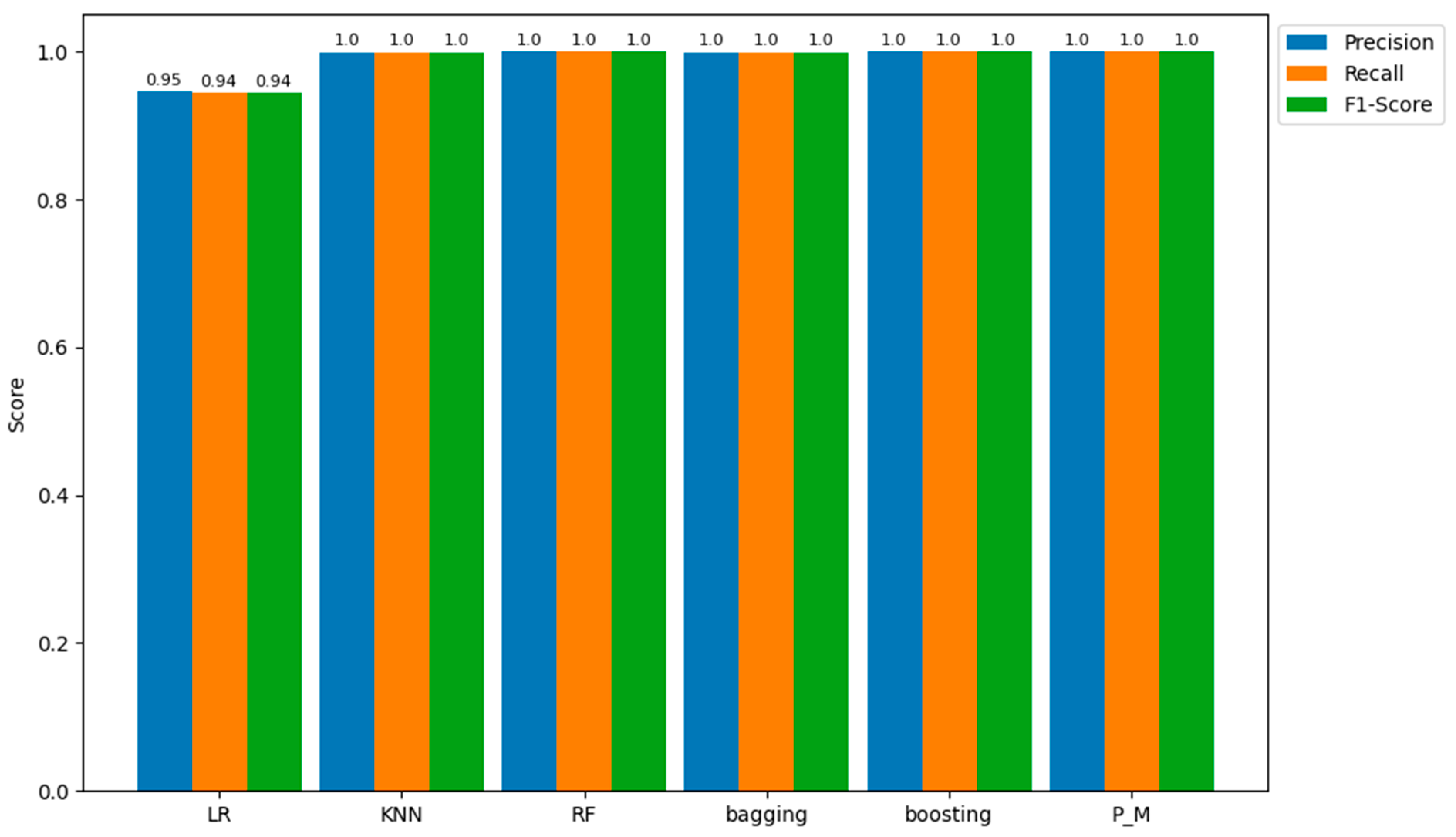
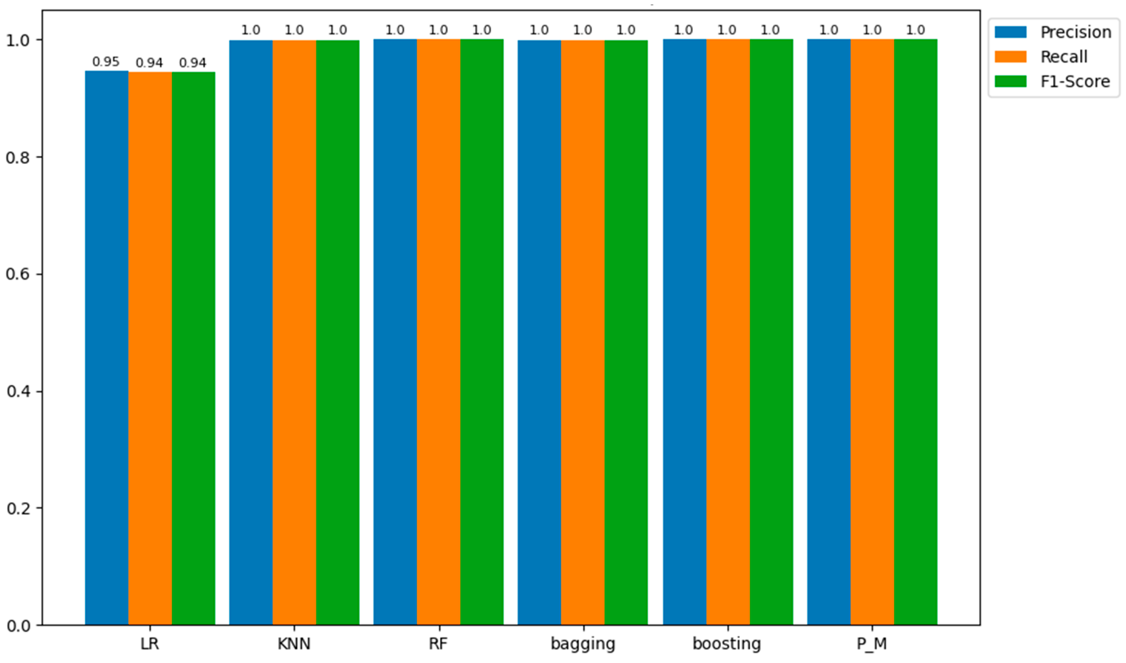
In a parallel evaluation of the results of the confusion matrix, we observe a consistent trend in the precision, recall, and accuracy metrics across our models when compared to both training and testing samples. Particularly, the majority of models have precision, recall, and accuracy scores that hover around 100 percent, demonstrating their proficiency in correctly classifying positive instances, as justified in Figure 12.

Based on the results and visual representations, it is evident that these models adeptly capture relevant data, leading to precise predictions and minimal false negatives. Despite this outstanding performance, the Logistic Regression (LR) model stands out with slightly lower yet commendable precision, recall, and accuracy scores of 95.0%. This distinction highlights the sensitivity of the LR classifier to specific data complexities while affirming the overall robustness of the results obtained by other classifiers. As mentioned earlier, the results for precision, recall, and F1-score obtained on both training and testing samples are consistent, as verified by the data presented in Table 12 and Figure 13.

Table 12. Precision, Recall and Accuracy of all models on Testing Sample of SMOTE dataset.

	LR	KNN	RF	Bagging	Boosting	PM
Precision	0.945938	0.999174	0.999891	0.999	0.999092	0.999601
Recall	0.944256	0.999173	0.99989	0.999	0.999092	0.9996
F1-score	0.944204	0.999173	0.99989	0.999	0.999092	0.9996

Figure 13. Precision, Recall and F1-Score comparison of models on the testing sample.

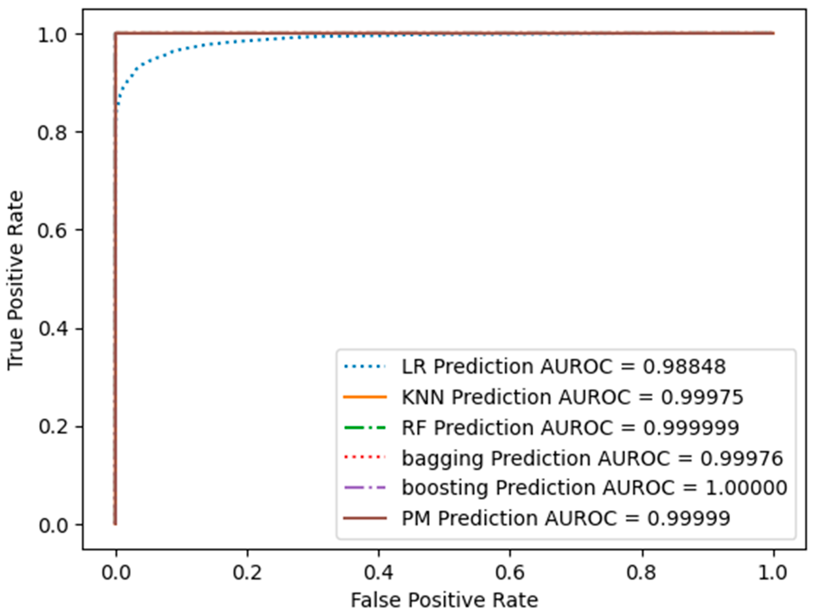
All ROC curves obtained from the SMOTE-sampled dataset, including Support Vector Machine (SVM), K-Nearest Neighbors (KNN), Random Forest (RF), Bagging, AdaBoost, and the proposed model (PM), exhibit exceptional performance, as indicated by the steep ascent towards the upper-left corner of the graph. This demonstrates that these models achieve high sensitivity while maintaining low false positive rates, highlighting their ability to classify positive instances while minimising misclassifications of negative instances accurately. Figure 14 shows the results of the ROC curve of all models, and the AUC-ROC values of all models are also shown in the bottom right corner.

The AUC-ROC values offer a quantitative assessment of the capability of the models. The AUC-ROC values, which range from 0.988 to 0.999, highlight the exceptional performance exhibited by all of the models. A higher AUC-ROC value indicates a stronger discriminatory ability of the model to distinguish between positive and negative events. In this comparative analysis, the AUC-ROC values continually converge towards or even attain a value of 1, validating the excellent predictive capacities exhibited by the models. The high AUC-ROC values observed in these models suggest a constant ability to predict genuine positives while effectively minimising false positives accurately. The combined utilisation of ROC curve analysis and the notable AUC-ROC values demonstrates the effectiveness of the models under consideration in accurately distinguishing between positive and negative occurrences.

4.2. Comparison with Existing Models

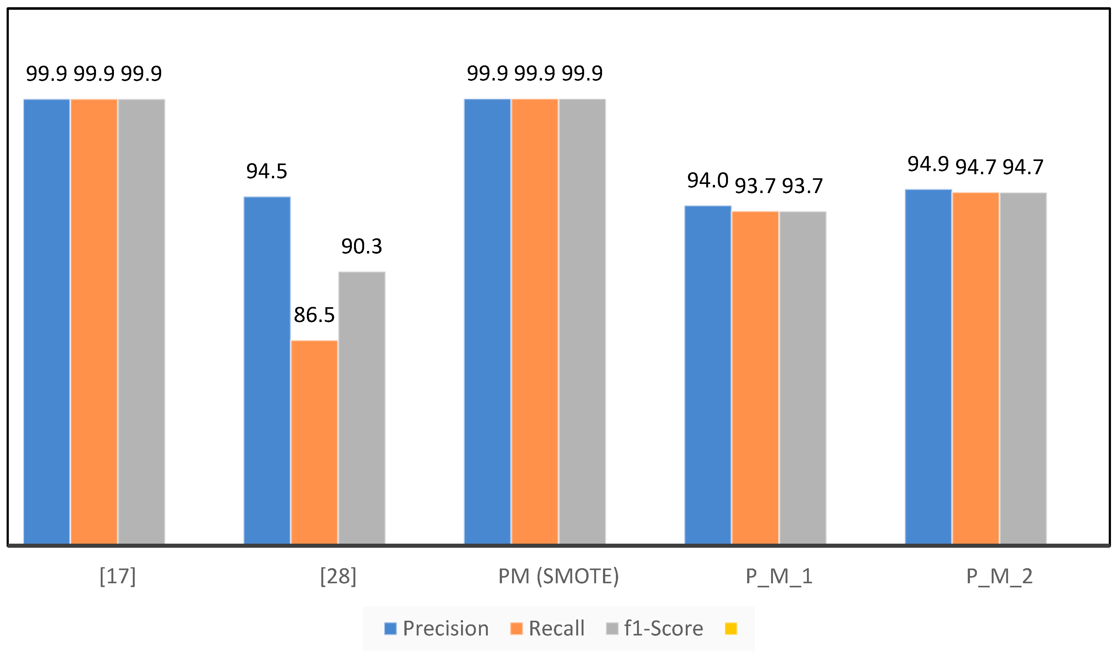
As in the literature review of this paper, different studies have been summarised in Table 1. The models proposed in [16,17] are comparable to the models proposed in this paper. In [16], the proposed model consists of a K-Nearest Neighbor (K-NN), Extreme Learning Machine (ELM), Random Forest (RF), Multilayer Perceptron (MLP) and Bagging classifier while the dataset used is different as used in this research. In [17], the proposed model contains Random Forest (RF), K-Nearest Neighbors (KNN), Logistic Regression (LR), Adaboost, and Bagging just like P_M_2 in under-sampling and PM in SMOTE. In [17], SMOTE is used for an unbalanced dataset, which is also used for our proposed model. Table 13 and Figure 15 show the evaluation metrics adopted for the benchmarking of the proposed model.

Table 13. Comparison of Proposed Model with Existing Research.

.	[17]	[28]	PM (SMOTE)	P_M_1	P_M_2
Accuracy	99.9455	83.83	99.9591	93.684	94.737
Precision	99.947	94.5	99.9591	93.996	94.916
Recall	99.9455	86.47	99.9591	93.684	94.737
F1-Score	99.9462	90.31	99.9591	93.673	94.731

Figure 15. Performance Comparison of the Proposed Model with Existing Models.

The accuracy achieved by the present model [28] is 83.83%, which is significantly lower compared to the accuracy achieved by our proposed model. This observation implies that there may be certain constraints in the accurate classification of cases, as shown by [24]. The proposed model in [25] has strong performance, with an accuracy percentage of 99.9455%. Although it demonstrates a high level of precision, it is crucial to consider additional measures in order to offer a thorough evaluation. The proposed model, PM (SMOTE), demonstrates exceptional performance with an accuracy of 99.9591%, exceeding the results achieved by both references [17,28]. This suggests that the PM (SMOTE) algorithm demonstrates a noteworthy capability in accurately classifying cases, perhaps leading to enhanced skills in fraud detection.

P_M_1 and P_M_2, two more models under consideration, exhibit comparable or somewhat inferior performance in accuracy, precision, recall, and F1-score when compared to the PM (SMOTE) model. The P_M_2 is the same model as PM; the only difference is the sampling technique used on the dataset. In P_M_2, under-sampling is used, while in the PM, SMOTE is used as a sampling technique. This implies that the utilisation of under-sampling as the sampling strategy in P_M_1 and P_M_2 may have resulted in a decrease in the size of the dataset. Although the process of reducing class distribution might contribute to achieving a balanced distribution in a class, it is important to acknowledge that this approach may lead to a certain degree of information loss. Consequently, the performance of this method may be comparatively poorer when compared to the PM (SMOTE) technique.

In summary, the assessment findings underscore the merits and limitations of different approaches. The PM (SMOTE) technique demonstrates superior performance, exhibiting the greatest levels of accuracy, precision, and F1 score. Nevertheless, it is crucial to consider the contextual factors and trade-offs that are linked to various sampling approaches. The utilisation of under-sampling, as seen in P_M_1 and P_M_2, might potentially impact the overall performance of the model. When selecting an appropriate model, it is important to consider the particular objectives and limitations associated with the work of credit card fraud detection.

Future Work

In future investigations, there is an opportunity to enhance the efficiency of the model. Despite the positive outcomes demonstrated by both our ensemble model and individual predictors, there remains a keen interest in refining their training and testing durations. Streamlining computing overhead holds the potential to develop fraud detection systems capable of real-time operation, ensuring swift responses to evolving fraud trends. While not the primary focus of this paper, exploring the potential integration of deep learning models is a worthwhile avenue. The exploration of designs such as Convolutional Neural Networks (CNNs) and Recurrent Neural Networks (RNNs), in conjunction with traditional machine learning methods, may yield more accurate and adaptable fraud detection solutions.

Conclusion

Our journey began with a comprehensive literature review that highlighted the severity of the credit card fraud issue. Identity theft, particularly through credit card fraud, has become alarmingly prevalent, causing innumerable victims' financial loss and emotional distress. The statistics presented by organisations such as the Federal Trade Commission (FTC) paint a bleak picture of the ever-changing landscape of fraud. To address these obstacles, a variety of fraud detection techniques were investigated. Statistical Analysis, Machine Learning, and Deep Learning Techniques were studied for transaction data and identifying suspicious patterns. For classification tasks, machine learning models ranging from K-Nearest Neighbors (KNN) to Support Vector Machines (SVM), Decision Trees (DT), Random Forest (RF), Bagging, and Boosting have emerged as formidable instruments. These models and their efficacy on a real-world database of European credit card transactions were carefully evaluated by our research.

All those efforts culminated in the proposal of an ensemble model that combines SVM, KNN, RF, Bagging, and Boosting classifiers within a voting framework. This ensemble not only demonstrated robust performance but also demonstrated the effectiveness of integrating multiple classifiers to increase the accuracy of fraud detection. During the evaluation phase, models in this paper were subjected to rigorous testing, and their performance was evaluated using a variety of metrics, including precision, recall, F1-score, ROC, and accuracy. The outcomes demonstrated the efficacy of our ensemble model in mitigating false positives and false negatives, two of the most significant obstacles in credit card fraud detection. However, this voyage also revealed research opportunities for the future. Maintaining a balance between accuracy and computational efficiency is essential.

Conflicts of Interest

The authors state that they do not have any competing financial interests or personal relationships that could potentially create biases or otherwise influence the research presented in this paper. The authors affirm that the work reported is free of any competing interests that could undermine the objectivity, integrity, or perceived validity of the paper.

References

National Crime Agency (NCA), "Fraud and Economic Crime." Accessed: May 11, 2023. [Online]. Available: https://www.nationalcrimeagency.gov.uk/what-we-do/crime-threats/fraud-and-economic-crime.
Federal Trade Commission, "CSN-Data-Book-2022," no. February 2023, Accessed: Mar. 11, 2023. [Online]. Available: https://www.ftc.gov/system/files/ftc_gov/pdf/CSN-Data-Book-2022.pdf.
A. Sudjianto, S. Nair, M. Yuan, A. Zhang, D. Kern, and F. Cela-D\’\iaz, "Statistical methods for fighting financial crimes," Technometrics, vol. 52, no. 1, pp. 5–19, 2010. [CrossRef]
S. Data, "Descriptive statistics," Birth, vol. 30, p. 40, 2012.
W. H. Walters, "Survey design, sampling, and significance testing: Key issues," The Journal of Academic Librarianship, vol. 47, no. 3, p. 102344, 2021. [CrossRef]
S. Lee and H. K. Kim, "Adsas: Comprehensive real-time anomaly detection system," in Information Security Applications: 19th International Conference, WISA 2018, Jeju Island, Korea, August 23–25, 2018, Revised Selected Papers 19, 2019, pp. 29–41.
M. Somvanshi, P. Chavan, S. Tambade, and S. V Shinde, "A review of machine learning techniques using decision tree and support vector machine," in 2016 international conference on computing communication control and automation (ICCUBEA), 2016, pp. 1–7.
R. Shah, "Introduction to K-Nearest Neighbors (kNN) Algorithm," https://ai.plainenglish.io/introduction-to-k-nearest-neighbors-knn-algorithm-e8617a448fa8.
S. D. Jadhav and H. P. Channe, "Comparative study of K-NN, naive Bayes and decision tree classification techniques," International Journal of Science and Research (IJSR), vol. 5, no. 1, pp. 1842–1845, 2016.
K. Randhawa, C. K. Loo, M. Seera, C. P. Lim, and A. K. Nandi, "Credit card fraud detection using AdaBoost and majority voting," IEEE Access, vol. 6, pp. 14277–14284, 2018. [CrossRef]
O. S. Yee, S. Sagadevan, and N. H. A. H. Malim, "Credit card fraud detection using machine learning as data mining technique," Journal of Telecommunication, Electronic and Computer Engineering (JTEC), vol. 10, no. 1–4, pp. 23–27, 2018.
S. Sengupta et al., "A review of deep learning with special emphasis on architectures, applications and recent trends," Knowl Based Syst, vol. 194, p. 105596, 2020. [CrossRef]
N. B. Muppalaneni, M. Ma, S. Gurumoorthy, P. R. Vardhani, Y. I. Priyadarshini, and Y. Narasimhulu, "CNN data mining algorithm for detecting credit card fraud," Soft computing and medical bioinformatics, pp. 85–93, 2019.
A. Roy, J. Sun, R. Mahoney, L. Alonzi, S. Adams, and P. Beling, "Deep learning detecting fraud in credit card transactions," in 2018 Systems and Information Engineering Design Symposium (SIEDS), 2018, pp. 129–134. [CrossRef]
U. Fiore, A. De Santis, F. Perla, P. Zanetti, and F. Palmieri, "Using generative adversarial networks for improving classification effectiveness in credit card fraud detection," Inf Sci (N Y), vol. 479, pp. 448–455, 2019. [CrossRef]
P. Y. Prasad, A. S. Chowdary, C. Bavitha, E. Mounisha, and C. Reethika, "A Comparison Study of Fraud Detection in Usage of Credit Cards using Machine Learning," in 2023 7th International Conference on Trends in Electronics and Informatics (ICOEI), 2023, pp. 1204–1209. [CrossRef]
G. L. Sahithi, V. Roshmi, Y. V. Sameera, and G. Pradeepini, "Credit Card Fraud Detection using Ensemble Methods in Machine Learning," in 2022 6th International Conference on Trends in Electronics and Informatics (ICOEI), 2022, pp. 1237–1241. [CrossRef]
R. Qaddoura and M. M. Biltawi, "Improving Fraud Detection in An Imbalanced Class Distribution Using Different Oversampling Techniques," in 2022 International Engineering Conference on Electrical, Energy, and Artificial Intelligence (EICEEAI), 2022, pp. 1–5. [CrossRef]
D. Tanouz, R. R. Subramanian, D. Eswar, G. V. P. Reddy, A. R. Kumar, and C. H. V. N. M. Praneeth, "Credit Card Fraud Detection Using Machine Learning," in 2021 5th International Conference on Intelligent Computing and Control Systems (ICICCS), 2021, pp. 967–972. [CrossRef]
R. Sailusha, V. Gnaneswar, R. Ramesh, and G. R. Rao, "Credit Card Fraud Detection Using Machine Learning," in 2020 4th International Conference on Intelligent Computing and Control Systems (ICICCS), 2020, pp. 1264–1270. [CrossRef]
I. Sadgali, N. Sael, and F. Benabbou, "Performance of machine learning techniques in the detection of financial frauds," Procedia Comput Sci, vol. 148, pp. 45–54, 2019. [CrossRef]
P. Raghavan and N. El Gayar, "Fraud Detection using Machine Learning and Deep Learning," in 2019 International Conference on Computational Intelligence and Knowledge Economy (ICCIKE), 2019, pp. 334–339. [CrossRef]
A. Saputra and others, "Fraud detection using machine learning in e-commerce," International Journal of Advanced Computer Science and Applications, vol. 10, no. 9, 2019. [CrossRef]
Y. Jain, N. Tiwari, S. Dubey, and S. Jain, "A comparative analysis of various credit card fraud detection techniques," International Journal of Recent Technology and Engineering, vol. 7, no. 5, pp. 402–407, 2019.
H. Naik and P. Kanikar, "Credit card fraud detection based on machine learning algorithms," Int J Comput Appl, vol. 182, no. 44, pp. 8–12, 2019.
D. Varmedja, M. Karanovic, S. Sladojevic, M. Arsenovic, and A. Anderla, "Credit Card Fraud Detection - Machine Learning methods," in 2019 18th International Symposium INFOTEH-JAHORINA (INFOTEH), 2019, pp. 1–5. [CrossRef]
A. Thennakoon, C. Bhagyani, S. Premadasa, S. Mihiranga, and N. Kuruwitaarachchi, "Real-time Credit Card Fraud Detection Using Machine Learning," in 2019 9th International Conference on Cloud Computing, Data Science & Engineering (Confluence), 2019, pp. 488–493. [CrossRef]
D. Prusti and S. K. Rath, "Fraudulent Transaction Detection in Credit Card by Applying Ensemble Machine Learning Techniques," in 2019 10th International Conference on Computing, Communication and Networking Technologies (ICCCNT), 2019, pp. 1–6. [CrossRef]
Machine Learning Group - ULB, "Credit Card Fraud Detection Dataset," https://www.kaggle.com/datasets/mlg-ulb/creditcardfraud.
Binh Vu, "Fraud ecommerce Dataset." 2018.
I. University of California, "KDD CUP 99 Intrusion Dataset." Accessed: Jun. 08, 2023. [Online]. Available: https://kdd.ics.uci.edu/databases/kddcup99/kddcup99.html.
I-Cheng Yeh, "Dataset," no. 2016. [CrossRef]
G. Niveditha, K. Abarna, and G. V Akshaya, "Credit card fraud detection using random forest algorithm," Int. J. Sci. Res. Comput. Sci. Eng. Inf. Technol, vol. 5, no. 2, pp. 301–306, 2019.
J. Graser, S. K. Kauwe, and T. D. Sparks, "Machine learning and energy minimisation approaches for crystal structure predictions: a review and new horizons," Chemistry of Materials, vol. 30, no. 11, pp. 3601–3612, 2018. [CrossRef]
Teemu Kanstrén, "A Look at Precision, Recall, and F1-Score." https://towardsdatascience.com.

Figure 1. Flow Diagram of Credit Card Fraud Detection using Machine Learning.

Figure 2. The Proposed Credit Card Fraud Detection Model.

Figure 3. The Architecture of the Proposed Credit Card Fraud Detection Model.

Figure 4. Visual Representation of Confusion Matrix.

Figure 5. Accuracy Results Comparison of all Models obtained on Training Sample.

Figure 6. Accuracy Results Comparison of all Models obtained on the Testing Sample Dataset.

Figure 7. Precision, Recall and F1-score of all Models on the Training Sample Dataset.

Figure 8. Precision, Recall and F1-score values of all Models obtained on the Testing Sample Dataset.

Figure 9. ROC Curve Plot of all Models on Testing Sample with AUC-ROC Value.

Figure 10. Accuracy Comparison of all models on Training Sample.

Figure 11. Accuracy comparison of all models on the Testing sample.

Figure 12. Precision, Recall and F1-Score comparison of models on the training sample.

Figure 14. ROC Curve and AUC-ROC Values of all Models.

Table 1. Comparison of ML Techniques used in Credit Card Fraud Detection Research.

Year	Authors	Ensemble ML Models	Under-Sampling	SMOTE	Comprehensive Evaluation
2019	Naik Kanikar [25]	✓	✓	×	✓
2019	Jain Tiwari et al. [24]	✓	✓	×	✓
2019	Saputra Suharjito [23]	✓	×	✓	✓
2019	Raghavan Gayar [22]	✓	×	✓	×
2019	Sadgali Benabbou [21]	✓	×	✓	×
2020	Sailusha Gnaneswar et al. [20]	✓	×	✓	×
2021	Tanouz Subramanian et al. [19]	✓	✓	×	✓
2022	Qaddoura, Biltawi [18]	✓	✓	✓	✓
2022	Sahithi Roshmi et al. [17]	✓	✓	×	✓
2023	Prasad Chowdary et al. [16]	✓	✓	×	✓
2023	Our Proposed Model	✓	✓	✓	✓

Table 2. Algorithm of the Proposed Credit Card Fraud Detection Model.

Algorithm	Credit Card Fraud Detection using Ensemble Machine Learning Models
Input:	Credit_Card_Fraud_Dataset
Output:	Trained_Machine_Learning_Models
1.	dataset ← Load_CreditCard_Fraud_Dataset()
2.	processed_data ← PreprocessedData(dataset)
3.	labels ← (processed_data)
4.	under_sampled_data ← (labels)
5.	smote_data ← (labels)
6. 7. 8. 9. 10. 11.	for model_type in [‘SVM’, ‘RF’, ‘Bagging’, ‘Boosting’, ‘LR’, ‘P_M_1’, ‘P_M_2’]: training_data, testing_data ← TrainTestSplit(under_sampled_data) if model_type == model: model ← model_type elif model_type == ‘Proposed_model’ models.append(mode_type)
12. 13. 14. 15.	for model_type, model in models: testing_data_features ← tresting_data.drop(‘Class’) testing_data_labels ← testing_data[‘Class’] confusion_matrix ← Evaluate_model(model, testing_data_features, testing_data_labels)
16.	endif
17.	end for
18.	return display_results ← (confusion_matrix, model_type)

Table 3. Confusion Matrix values for Training sample.

	SVM	KNN	RF	Bagging	Boosting	P_M_1	LR	P_M_2
True Positive	345	345	378	344	378	354	349	358
True Negative	372	372	378	371	378	378	371	378
False Positive	33	33	0	34	0	24	29	20
False Negative	6	6	0	7	0	0	7	0

Table 4. Confusion Matrix values for Testing Sample.

	SVM	KNN	RF	Bagging	Boosting	P_M_1	LR	P_M_2
True Positive	87	86	86	87	86	85	87	87
True Negative	92	92	93	93	92	93	90	93
False Positive	8	9	9	8	9	10	8	8
False Negative	3	3	2	2	3	2	5	2

Table 5. Accuracy results of all Models on Training and Testing Samples Dataset.

Training Sample of Under-Sample Dataset
	SVM	KNN	RF	Bagging	Boosting	P_M_1	LR	P_M_2
Accuracy	0.96	0.951	1	0.95	1	0.97	0.955	0.97
Testing Sample of Under-Sample Dataset
Accuracy	0.9421	0.9368	0.937	0.9473	0.9368	0.9368	0.9315	0.9473

Table 6. Precision, Recall and F1-score of all Models on the Training Sample Dataset.

	SVM	KNN	RF	Bagging	Boosting	P_M_1	LR	P_M_2
Precision	0.961	0.955	1	0.953	1	0.971	0.957	0.971
Recall	0.96	0.951	1	0.95	1	0.97	0.955	0.97
F1-score	0.96	0.951	1	0.95	1	0.97	0.955	0.97

Table 7. Precision, Recall and F1-score on Testing Sample of Under-Sample Dataset.

	SVM	KNN	RF	Bagging	Boosting	P_M_1	LR	PM2
Precision	0.942	0.945	0.939	0.939	0.945	0.945	0.948	0.949
Recall	0.942	0.942	0.937	0.937	0.942	0.942	0.947	0.947
F1-score	0.942	0.942	0.937	0.937	0.942	0.942	0.947	0.947

Table 8. Confusion Matrix of all Models obtained on Training Sample of SMOTE Dataset.

	LR	KNN	RF	Bagging	Boosting	P_M
True Positive	201231	220152	220152	220152	220152	220152
True Negative	214606	219868	220152	219864	220152	220082
False Positive	18921	0	0	0	0	0
False Negative	5546	284	0	288	0	70

Table 9. Confusion Matrix of all Models obtained on Testing Sample of SMOTE Dataset.

	LR	KNN	RF	Bagging	Boosting	P_M
True Positive	50280	55038	55038	55038	55038	55038
True Negative	53660	54947	55028	54941	55028	54993
False Positive	4758	0	0	0	0	0
False Negative	1378	91	10	97	10	45

Table 11. Precision, Recall and F1-score of all models on Training sample of SMOTE dataset.

Prediction Results on Training Sample of SMOTE Dataset
	LR	KNN	RF	Bagging	Boosting	PM
Precision	0.94607	0.999355	1	0.9993	1	0.99983
Recall	0.94443	0.99954	1	0.9993	1	0.999831
F1-score	0.94438	0.99954	1	0.9993	1	0.999831

Disclaimer/Publisher’s Note: The statements, opinions and data contained in all publications are solely those of the individual author(s) and contributor(s) and not of MDPI and/or the editor(s). MDPI and/or the editor(s) disclaim responsibility for any injury to people or property resulting from any ideas, methods, instructions or products referred to in the content.

© 2023 by the authors. Licensee MDPI, Basel, Switzerland. This article is an open access article distributed under the terms and conditions of the Creative Commons Attribution (CC BY) license (http://creativecommons.org/licenses/by/4.0/).

Copyright: This open access article is published under a Creative Commons CC BY 4.0 license, which permit the free download, distribution, and reuse, provided that the author and preprint are cited in any reuse.

MDPI Initiatives

Important Links

Choose an area of interest and we will send you notifications of new preprints at your preferred frequency.

Disclaimer