REFS - A Risk Evaluation Framework on Supply Chain

Preprint

Article

REFS - A Risk Evaluation Framework on Supply Chain

Altmetrics

Downloads

Views

Comments

A peer-reviewed article of this preprint also exists.

Istvan Mihalcz^*

This version is not peer-reviewed

Submitted:

13 December 2023

Posted:

14 December 2023

You are already at the latest version

Alerts

Abstract

In contrast to its traditional form, in which large, powerful companies were solely and exclusively responsible for supplies, manufacturing, and distribution, the supply chain has undergone substantial change over the past half-century. Today, nearly all supply chain processes are outsourced, thanks to the efforts of innovative, modern companies. The degree of risk associated with contemporary supply chains is greater than the majority of supply chain managers acknowledge, according to an accumulation of studies, analysts, and news outlets. Vulnerabilities within the supply chain remain a significant challenge for numerous organizations. Inadequate management of these risks—which include, but are not limited to, natural disasters, acts of terrorism, cyber assaults, the credit crisis, pandemic scenarios, and war—could lead to significant declines in profitability, productivity, revenue, competitive advantage, and other metrics. Concerns regarding the risk assessment of the supply chain remain unresolved. The objective of this article is to present a risk evaluation framework that can be effectively implemented in the assessment of supply chain risks. This study makes a fundamental contribution to the body of knowledge by providing supply chain managers with a practical instrument for assessing their processes, irrespective of the mathematical underpinnings or the diverse variables employed in risk assessment. A case study from an automotive EMS production is used to compare the outcomes of multiple aggregation methods; the conclusions are then validated by risk and FMEA specialists from the same factory.

Keywords:

Subject: Business, Economics and Management - Business and Management

1. Introduction

In the past decade, numerous organizations have incurred expenses amounting to hundreds of millions of dollars or euros due to unforeseen disruptions and weaknesses in their supply chains. At the heart of these problems is the absence of dependable mechanisms to identify and effectively mitigate the escalating supply chain risks that result from increased global interconnectedness. As a consequence, the evaluation of supply chain risk is progressively gaining importance. There has been an exponential increase in the quantity of risk analysis papers published since the beginning of the century [1]. Considering the quantity of scholarly articles dedicated to the most widely used risk analysis techniques and pragmatic implementations of FMEA in diverse domains, the supply chain would rank last on this list [1]. Notwithstanding this, a multitude of concerns pertaining to the FMEA methodology continue to be unresolved in the recently published FMEA (released in [2]). In regard to supply chain risk analysis, there remain uncharted territories.

The evaluation and selection of suppliers are critical components of the supply chain. Dickson established the initial classification system in 1966 [3], and Cheraghi subsequently revised it in 2011 [4]. Huang et al. [1] published a systematic literature review in 2021 that demonstrates the exponential growth of risk analysis publications over the past two decades. Keyword analysis reveals that "FMEA", "system", "risk evaluation", "criticality analysis", and "failure mode" have risen to prominent positions. Similar findings were published by Liu et al. [5] in 2013. It can be concluded that the FMEA continues to be the most widely utilized tool for risk assessment; however, it is presently employed in conjunction with alternative evaluation approaches [1,5].

Several authors [6,7,8] have explored the factors contributing to the infrequent utilization of FMEA and other risk analysis approaches within the supply chain. The researchers conducted an investigation and successfully identified the underlying factors: the primary obstacle hindering broader implementation seems to stem from a deficiency in comprehending the application of FMEA within a supply chain context.

Numerous scholarly articles have highlighted the limitations of the FMEA [5,9,10,11].

The AIAG-VDA FMEA 1st Edition, a novel FMEA framework, was published in the year 2019 [2]. The recent update to the system includes the addition of a chapter titled "Monitoring and System Response." In this update, the Risk Priority Number (RPN) has been replaced with Action Priority Tables. Furthermore, a comprehensive approach consisting of seven steps, namely planning, structure analysis, function analysis, failure analysis, risk analysis, optimization, and documentation of results, has been implemented. The utilization of the Severity (S), Occurrence (O), and Detection (D) scales persists, and it is advisable for the team to evaluate them in a manner consistent with a conventional FMEA. The utilization of the Action Priority Level, which is determined based on the values of the S, O, and D components from a designated Action Priority Table, has replaced the use of RPN. The table for AP levels, which is suggested, is derived from the values assigned to the components S, O, and D. However, it is subject to modification based on factors such as the nature of the business, the specific process, or the industry involved. The AP table delineates the instances in which the organization is authorized to initiate action, as opposed to the responsibility falling upon the FMEA Team. No action is required for Low AP levels, while any lack of action for Medium AP levels should be adequately justified. In the case of High AP levels, immediate action must be taken to mitigate the risk. This suggests that instead of relying on the RPN value, the actions are selected based on the specific values of the factors. Regrettably, as evidenced in Table A6, the current system is incapable of accurately discerning the actual amount of risk.

It may be inferred from the existing body of research that the supply chain industry use risk analysis methods that closely resemble those employed in various other domains. The authors exclusively employ the FMEA [12,13,14] assessment technique, or a modified version of FMEA with factors limited to 5 levels instead of 10 [15]. Alternatively, they utilize mixed evaluation techniques such as Fuzzy-FMEA [11,16,17,18,19], Fuzzy-AHP [20,21], FMEA-ANP [22], or Fuzzy Bayesian-based FMEA [14]. Fuzzy FMEA [19] is considered the second most often utilized risk analysis technique, following the FMEA method. The three membership functions commonly utilized in Fuzzy FMEA are triangular, trapezoidal, and Gaussian [23,24,25].

The conventional approach for assessing supply chain risk predominantly involves employing the FMEA framework, which incorporates three key factors: Severity, Occurrence, and Detection. A limited number of authors argue against the adequacy of three factors and instead propose the utilization of models that incorporate either four (expense, time, flexibility, and quality) [26] or five (likelihood, consequence of time/delay, consequence of additional expense, consequence of damage to quality, and visibility) [27] factors. In the present case, commonly employed variables were assessed, namely Visibility and Consequence, with the latter being determined by the provider’s delay, cost associated with the supplier, and the quality of the given components.

In the context of supply chain risk analysis, new factors have emerged, such as Quality, Time, Cost [14,26], Intensity [13], Consequence [8], Effect, Cause, Measure [28], and others.

The aggregation function of multiplication remains the most frequently employed method when examining the utilization of aggregation functions in the context of [6,7,8,21,28]. The second approach integrates Fuzzy analysis with FMEA [11,16,17,20].

The exposure of businesses, irrespective of their industry, to both internal and external risks is evident through supply chain disruption. This document does not provide an exhaustive compilation of potential failures; rather, it presents a limited number of illustrative instances.

Internal supply chain interruption can potentially arise due to:

Instances of internal operational disruptions,
Instances of significant management, staff, and operational procedure changes,
Instances of failure to implement contingency plans in response to problems,
Instances of inadequate implementation of cybersecurity policies and controls leading to cyberattacks and data breaches,
Instances of non-compliance with labor laws or environmental standards,
Instances of unavailability of products to meet customer demands (attributable to inventory issues, ERP system malfunctions, human errors, etc.).

The external supply chain risk might arise due to factors such as:

Unpredictable or misunderstood consumer demand,
Delays in the transportation and distribution of commodities, encompassing many types such as components, finished products, and raw materials,
The potential risks posed by terrorism, armed conflict, economic or political penalties, as well as social, governmental, and economic challenges,
The management of supplier risk include concerns regarding the physical infrastructure and regulatory compliance of a supplier,
Natural disasters, such as tornadoes, hurricanes, and earthquakes,
Human errors occur at all levels and in all locations.

In summary, there is a dearth of a relevant, practical, and flexible instrument for conducting supply network risk evaluations. This tool should be easily accessible to supply chain managers and risk analysts, considering the aforementioned activities and global developments affecting the supply chain. This tool ought to enhance its effectiveness in identifying authentic threats, encompass a broader range of risk variables beyond the current limit of three, and maintain a level of user-friendliness comparable to that of the conventional FMEA methodology.

This article undertakes a comprehensive literature study on supply chain risk management approaches and presents a summary of the various types and extent of elements considered. The paper examines supplementary aggregation methodologies for situations involving numerous components, beyond three in number, by building upon the widely adopted FMEA as a foundational framework. Additionally, this study conducts a comparative examination of several risk analysis methodologies within the context of the flexible TREF-based risk evaluation framework ([29,30]). The framework is further enhanced by incorporating the Fuzzy-FMEA approach, and the techniques are subsequently ranked using the TOPSIS method. This paper presents a case study that investigates the analysis of supply chain risks in an automotive manufacturing service firm, primarily focusing on Tier 2 suppliers. The company is situated in a central position within the supply chain, making it an ideal subject for examining the practical implementation of this analytical approach. The experienced staff of the organization validates the supplied approach by doing a comparative assessment with the provided instrument.

2. Mathematical background

2.1. Aggregation functions criteria

In the study conducted by the authors in [31,32,33], various aggregating functions were examined. Additionally, in [31], the authors provided an analysis that included critique of the Risk Priority Number (RPN). Aggregation functions necessitate several conditions, including validity, monotonicity, sensitivity, symmetricity, linearity, scale fit, and scale endpoint identity.

Validity: Consider the manner in which the risk emanates from the constituents.

$F : I^{n} \to R; x \in I^{n}; a, b \in R; F (x) = a, a n d F (x) = b \Rightarrow a = b$

(1)
Monotonicity: refers to the property of a function where it exhibits nondecreasing behavior, meaning that it yields a nonnegative reaction to any increase in its arguments. In other words, the function does not reduce its output value when any input value is increased.

$F : I^{n} \to R x, x^{'} \in I^{n}, x \geq x^{'} \Rightarrow F (x) \geq F (x^{'})$

(2)

The membership functions and the defuzzification function employed in this study exhibit monotonic characteristics..
Sensitivity refers to the degree of responsiveness or reactivity exhibited in a certain context. In the specific scenario of rigorous monotonicity, sensitivity pertains to the extent to which a change in one variable directly and consistently influences a change in another variable.

$F : I^{n} \to R i \in [n] F (x) \neq F (x + λ) x \in I, λ \neq 0 x + λ \in I$

(3)
The property of symmetricity, also known as commutativity, is true when the components or elements of a distribution follow a symmetric distribution. In such cases, the distribution of the aggregated values also exhibits symmetry. This property is also observed in the Fuzzy functions employed.

$F : I^{n} \to R F (x) = F (| x |)$

(4)
Linearity refers to the property where, in the scenario of components or factors adhering to a uniform distribution, the resulting distribution of the aggregated values will also exhibit uniformity.
Scale fitting: The aggregate processes should be conducted using the scale values that have been applied. This criterion is also met as the range of each factor is identical.
Scale endpoint identity: In order to adhere to the boundary criteria, the endpoints of the scales were modified to fall within the interval [1, 10]. This adjustment was important as it ensured that each factor’s potential values were defined within the same range.

2.2. Risk aggregation functions

Definition 1.

Let

f = {[f_{1}, f_{2}, . ., f_{n}]}^{T}

(n \geq 3)

be the vector representing the set of risk factors. Let

r = S (f)

represent the resulting risk value, where S is a monotonous aggregation function. The risk aggregation protocol (RAP) is denoted as

(f, S)

Remark 1.

It is commonly assumed that the risk factors

f_{i}

and

f_{j}

, where

(i \neq j)

are independent of one another. Nevertheless, the proposed RAP does not need its independence.

According to the provided definition, the quantity of factors, including severity, detection, incidence, cost, and others, is denoted by the variable

n \in {3, 4, 5, . . .} \in R^{+}

. The risk ranking numbers, denoted as

f_{i} \in {1, 2, . ., 10}

are related to factor i. This input will be employed by aggregation functions to evaluate each risk case.

Several instances of aggregation functions S are as follows:

$S_{1} (f) = \prod_{i : = 1}^{n} f_{i}$ is the geometric mean of risk factors. If n=3, and the factors are severity, occurrence, and detection, we have the original RPN (risk priority number) from the FMEA.
$S_{2} (f) = M e d i a n ({f})$ is the median of risk factors.
$S_{3} (f) = \frac{1}{n} \sum_{i : = 1}^{n} f_{i}$ is the average of risk factors.
$S_{4} (f) = \sqrt{\sum_{i : = 1}^{n} f_{i}^{2}}$ is the generalized n-dimensional radial distance of risk factors.
$S_{5} (f) =$ Aggregation of Fuzzy membership functions based on rule base

The utilization of risk analysis inside the supply chain is not as prevalent as it ideally should be, primarily due to a lack of competence among purchasing, procurement, and logistics managers, as evidenced in the preceding chapter. The risk assessment framework, known as [29], has undergone an expansion to incorporate a fuzzy module. This addition has been implemented to effectively address the issue at hand.

2.3. Implementation of Fuzzy

The approach that was taken with the previously disclosed Fuzzy aggregation function will remain unchanged. Fuzzy logic consists of three phases, the first of which is Fuzzyfication/Fuzzyfier, which transforms the factors into fuzzy variables. Inference, which follows, generates output fuzzy variables through the application of the Fuzzy rule base to input fuzzy variables. This component may be regarded as a protocol for aggregation. During the final stage, Defuzzyfication/Defuzzifier, the output is converted back into authentic output variables, which in this case are the risk level and/or value.

2.3.1. Fuzzyfication/Fuzzyfier

Initially, it is necessary to define the input fuzzy variables by employing the input membership functions. This implies that fuzzy membership functions should be used to convert each risk factor into an input fuzzy variable. The designation for these values is "crisps." A multitude of linguistic variables influence the number of membership functions associated with a given variable. Typically, Fuzzy FMEA utilizes three to seven linguistic variables ([34,35]). It is possible to incorporate additional variables; however, in the given context, the rule base became exceedingly intricate. In the beginning, the input fuzzy variables must be defined through the utilization of input membership functions. Accordingly, each risk factor should be converted into an input fuzzy variable utilizing fuzzy membership functions. These qualities are referred to as "crisps." The count of membership functions attributed to a specific variable is influenced by an abundance of linguistic variables. Fuzzy FMEA generally employs between three and seven linguistic variables ([34,35]). Although it is feasible to include further variables, doing so would have rendered the rule base significantly complex in the given context.

At the beginning and ending of the interval, the sigmoid function was implemented:

μ {(x, a, b)}_{s i g u} = \{\begin{matrix} 0, x \leq a \\ \frac{1}{1 + e^{a (x - b)}}, & any other case \end{matrix}

(5)

μ {(x, a, b)}_{s i g d} = \{\begin{matrix} 1 - \frac{1}{1 + e^{a (x - b)}}, x \leq a \\ 0, & any other case \end{matrix}

(6)

where a is the steepness of function, and b is the inflection point.

For each range within the interval, the bell/splay function is applied:

μ {(x, a, b, c)}_{s p l} = \frac{1}{1 + | \frac{x - b}{a} |^{2 c}}

(7)

where b is the center of function, a is the width of curve and c is the steepness of function.

Both the splay and bell are Gaussian membership functions that were selected due to their smoothness, nonzero value at all point intervals, continuous differentiability, and mathematical and computational tractability [25].

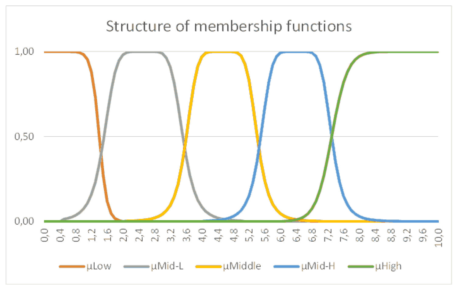
As illustrated in Figure 1, for n=5 (5 linguistic levels), in accordance with its original score or crisp, each component is converted into the sum of n membership functions.

S_{i} (f_{i}) = \sum_{i : = 1}^{n} μ_{i} (x)

, x ≤ 10 and

x \in R^{+}

, other variables of membership functions are constants (a, b, c).

Each factor will have its own sum of membership functions, noted

S_{i} (f_{i}), f_{i} \in {1, 2, . ., 10} \in N

, representing the ranking of risk converted in a number.

2.3.2. Fuzzy rule base

An analogy can be drawn between the sum of the fuzzy membership functions and the accumulation of factors comprising the fuzzy rule base. The literature also contains considerable variation regarding the selected aggregation method for fuzzy sets: only sums, products, maximal functions, or the Mamdani Fuzzy Inference (MFI) are employed due to the more comprehensible and intuitive nature of their rule bases. The MFI functions optimally in expert system applications in which the norms are established based on the expertise possessed by human beings. The input of this aggregation consists of fuzzy sets, and the output is also a fuzzy set. The output is determined by the center of mass or gravity, and the rule basis is a simple IF-THEN structure. An instance of this can be described as follows:

W_{i} (S_{i}) = S_{1} (f_{i}) \otimes S_{2} (f_{j}) \otimes . . . \otimes S_{n} (f_{n})

(8)

where ⊗ is the aggregation protocol.

2.3.3. Defuzzyfication

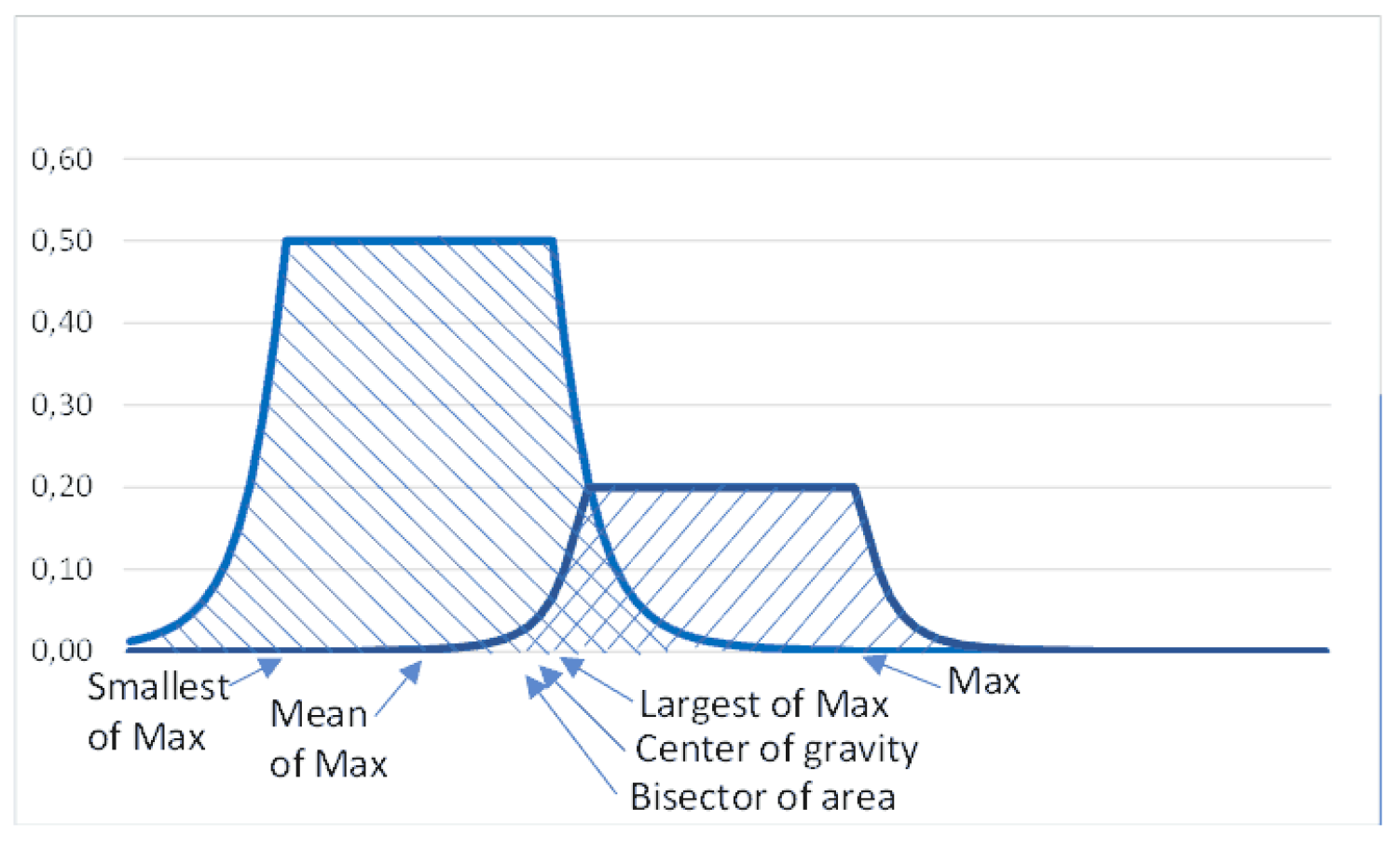
The final phase entails the transformation of the amount of risk from a fuzzy state to a crisp state. In this phase, the determination of risk level will be achieved by numerically converting the membership functions, which subsequently produce outcomes. There exist several viable defuzzification strategies, including:

Center of gravity of area - see Figure Figure 2),
Bisector of area refers to a vertical line that partitions a fuzzy set into two sub-regions of equivalent area. The phenomenon in question may exhibit alignment with the center of gravity, however this correlation is not universally observed.
Mean of Max level,
Largest of Max - the max value of the highest output membership function,
Max - the max limit value achieved by any output function,
Smallest of Max - the lowest value of the highest output membership function,
Low - is the lowest value achieved by any output function.

The computation of the center of gravity of the membership function is performed, considering the factor’s value, and subsequently, the results are aggregated.

x_{i} = \frac{\int μ_{C} (x) x d x}{\int μ_{C} (x) d x}

(9)

\int μ_{C} (X) d x

represents the measure of the region enclosed by the membership function C. If the parameter

μ_{C}

is established based on multiple discrete membership functions, the center of gravity can be mathematically represented as the summation of these functions.

x_{i} = \frac{\sum_{i = 1}^{N} μ_{C} (x_{i}) x_{i}}{\sum_{i = 1}^{N} μ_{C} (x_{i})}

(10)

In actuality, it is feasible to explicitly determine the center of gravity of membership functions by clearly describing the functions. The following diagram presents a visual representation of the methodologies employed in the calculation of accurate output (Figure 2).

The case study utilized the center of gravity approach.

The outputs of the different models are scaled by a constant factor to ensure that they possess a comparable range to other techniques.

It can be said that the utilized Fuzzy function, encompassing the process of defuzzification, meets all the requisite conditions for an aggregate function as delineated by the six criteria earlier expounded upon (Chapter 2.1).

2.4. Rank correlation

Spearman’s rank correlation coefficient defines the measure of rank correlation:

r_{s} = 1 - \frac{6 \sum_{i = 1}^{N} {(R_{X_{i} - R_{Y_{i}}})}^{2}}{N (N^{2} - 1)}

(11)

where

R_{X_{i}}

and

R_{Y_{i}}

represent the ranks of the first and second variables, respectively. The Spearman’s rank correlation coefficient is a statistical measure that quantifies the strength and direction of the association between two variables. The sign and magnitude of the value both fall within the range of

[- 1; + 1]

2.5. TOPSIS (Technique for Order Preference by Similarity to Ideal Solution)

The application of a multi-criteria decision analysis technique will be employed to evaluate a set of alternatives and ascertain the ranking of the risk analysis models implemented. The TOPSIS method chooses the alternative that has the shortest geometric distance from a positive ideal solution and the greatest geometric distance from a negative ideal solution [36].

Let A represent the pairwise comparison matrix for factors as follows:

A = (\begin{matrix} a_{1_{1}} & \dots & a_{1_{n}} \\ \dots & \dots & \dots \\ a_{n_{1}} & \dots & a_{n_{n}} \end{matrix})

(12)

where

a_{i_{j}}

are the judgement scores, considering

a_{i_{j}} = 1 / a_{j_{i}}

, and

a_{i_{i}} = 1

. This matrix is normalized with:

k_{i_{j}} = \frac{a_{i_{j}}}{\sum_{j = 1}^{n} a_{i_{j}}}

(13)

The local weight resulting:

w_{i} = \sum_{j = 1}^{n} \frac{k_{i_{j}}}{n}

(14)

The variables

h_{i}

are used to represent the risk incidents, where i ranges from 1 to n. Similarly, the variables

f_{j}

are employed to designate the TOPSIS evaluation criteria, with j ranging from 1 to m. The numerical outcomes of the alternative

h_{i}

with respect to the criteria

f_{j}

are represented by the variable

x_{i_{j}}

. The formula for the normalized decision matrix can be expressed as follows:

d_{i_{j}} = \frac{x_{i_{j}}}{\sqrt{\sum_{j = 1}^{m} x_{i_{j}}^{2}}}

(15)

The weighted normalized decision matrix elements can be generated:

V_{i_{j}} = w_{i} \times d_{i_{j}}

(16)

The ideal best solution

V_{j} +

and ideal worst solution

V_{j} -

are determined by aggregating the highest and lowest values of each criterion.

For beneficial criteria:

V_{j}^{+} = m a x [V_{i_{j}}] V_{j}^{-} = m i n [V_{i_{j}}]

(17)

For non-beneficial criteria:

V_{j}^{+} = m i n [V_{i_{j}}] V_{j}^{-} = m a x [V_{i_{j}}]

(18)

Euclidian distances are measured from the ideal best (

S_{i}^{+}

) and ideal worst (

S_{i} -

) values:

S_{i}^{+} = \sqrt{\sum_{j = 1}^{m} {(V_{i_{j}} - V_{j}^{+})}^{2}} S_{i}^{-} = \sqrt{\sum_{j = 1}^{m} {(V_{i_{j}} - V_{j}^{-})}^{2}}

(19)

The performance score (relative closeness to the ideal solution) can be calculated:

P_{i} = \frac{S_{i}^{-}}{S_{i}^{+} + S_{i}^{-}}

(20)

The ranked options are subsequently arranged in descending order as the final step.

This methodology is suitable for pairwise correlation analysis, specifically when the number of variables being compared does not exceed seven. Implementing this strategy gets problematic in situations where there are more than ten hazards, which is a frequently seen phenomenon in real-world scenarios. An illustration depicting the initial use of the Technique for Order of Preference by Similarity to Ideal Solution (TOPSIS) may be observed in the [37] context.

When evaluating a case that involves more than seven significant individual hazards, it is recommended to engage a team of experts that possess comprehensive expertise regarding the consequences associated with each risk. The individuals possess the capability to produce a matrix that facilitates the rating of effects, dangers, and impacts, alongside another matrix that enables the evaluation of results. One can utilize RSTUDIO to input both matrices and calculate their ranks using the TOPSIS algorithm [38].

3. Case study

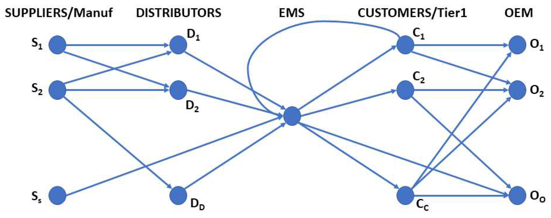
The study’s experimental focused on an electronic manufacturing services (EMS) supplier. Conducting testing within the comprehensive supply chain offers several advantages owing to the central location of the EMS (see Figure 3).

In certain instances, manufacturers

(S_{x})

or, in extreme circumstances, direct customers

(C_{x})

are occasionally chosen as the source for larger quantities of raw materials or components, despite the customary practice of EMS firms to procure them via distributors

(D_{x})

. This holds particularly true in cases when the design of the final product is still undergoing development or when it becomes imperative to conduct tests on updated components. To facilitate the installation of these units by original equipment manufacturers (OEMs), the EMS delivers the goods to direct customers

(C_{x})

. Subsequently, these customers engage in further processes, such as the development of more intricate modules, testing, and programming.

Under some circumstances, the EMS may also provide the carmaker with goods directly, as indicated by the

E M S - O_{x}

connection in Figure 3. The instances of

S_{x}

and

D_{x}

have been simplified in the EMS. They are treated as a single node or "location" because the EMS communicates with them through their Distribution Centers or offices, even though they consist of several factories/locations. Various logistical groups play a crucial role in facilitating the transportation of products between different nodes throughout the process. This case study offers a comprehensive opportunity to analyze a wide range of supply chain issues.

The automotive industry places significant importance on the availability of raw materials for manufacture, ensuring that they are provided in the appropriate time, quantity, and quality. Additionally, the industry recognizes the need for problem-free production, which is not the focus of this study, and the timely and accurate delivery of products to customers. Any departure from this stipulation leads to supplementary costs or a decrease in revenue.

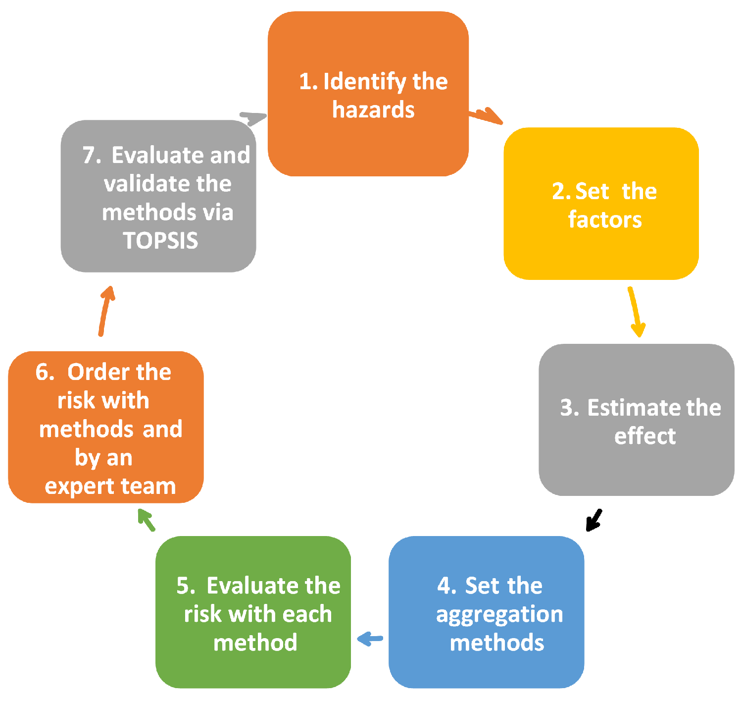
The assessment stages are depicted in Figure 4, and they are employed in both the case study and the subsequent discussion of the theoretical framework underlying this methodology.

A team of professionals specializing in logistics, quality management, risk assessment, and FMEA was assembled within the EMS firm. The primary objective of this team was to conduct comprehensive testing, analysis, and validation of the entire approach. The establishment of such a team inside any automotive industry is facilitated by the requirement of their Quality Management System (QMS) to do so. The initial step, denoted as Step 0, might be conceptualized as the establishment of the team.

Step 1: The present study conducted an exhaustive analysis of various supply chain concerns, including claims, losses, and delays, spanning a period of four years. Subsequently, a comprehensive inventory of risks was compiled. In this particular case, a total of 20 unique concerns were identified.

Step 2: The criteria for evaluating each factor, specifically Occurrence, Severity, and Detection, are presented in Table A1, Table A2, and Table A3 respectively. These tables may be found in the Appendix. The quantity of factors is contingent upon the intricacy of the business or logistic procedures, traffic patterns, business affiliations, and other pertinent considerations. It is imperative to assess these factors on a case-by-case basis for each company, as the level of risk may vary depending on factors such as geographical location, supply chain network, technological infrastructure, workforce availability and expertise, environmental conditions, and core technological capabilities. A severity rating was established to assess the most severe consequences resulting from a particular failure, with respect to both direct customers and OEMs. The decision should be made without considering the incidence, identification, or other relevant factors.

Step 3: The findings of the FMEA analysis, considering the aforementioned criteria, are presented in Table A6. The result was generated by employing both the previous FMEA standard, which solely considered the initial three factors (Occurrence, Severity, and Detectability), and the present FMEA standard that included AP (Action Priority) levels.

The maximum RPN (Risk Priority Number) score observed in this particular instance for manual handling procedures is 162. This value slightly surpasses the commonly employed risk threshold. In the context of ISO9001, this threshold is typically regarded as the midpoint within the range of factors, resulting in a value of 125 for three factors (

5^{3} = 125

). In the automotive/IATF16949 industry, companies individually define this limit, which generally falls around 100 or lower, as determined by management. Moreover, when the most severe and imperceptible process flaw are amalgamated with a significantly low occurrence score, the Risk Priority Number (RPN) will amount to 100 (1x10x10), a value that falls below the commonly employed action criterion threshold by several firms. The implementation of the updated FMEA methodology will yield a marginally more accurate outcome. However, its effectiveness remains inadequate as the risk level was merely ty of implementing risk mitigation measures. If individuals are not justified, it is imperative that they become justified.

Table A6 illustrates three factors that are insufficient in appropriately highlighting the true level of threat. This is the reason why certain authors and researchers have started incorporating supplementary variables (such as doing analysis with four or five components).

Every organization has the autonomy to make a decision regarding whether to accept, mitigate, or acknowledge specific hazards. Based on the aforementioned information, the management of the company or the team of experts can ascertain the specific aspects that accentuate the level of risk. The upper echelons of management within this EMS company were engaged in consultation, resulting in the selection of two more elements, namely control and cost.

The cost refers to the estimated financial impact incurred due to errors or inefficiencies in handling or logistics. Within the realm of literature, this particular element is commonly referred to as "Value."

The second factor is the Control factor, which assesses the feasibility and effectiveness of controlling, preventing, or mitigating a process, and determines the extent to which it can be achieved. Please refer to Table A4 and Table A5 for a comprehensive overview of the established evaluation criteria pertaining to the supplementary components.

Step 4: The present set of factors include Severity, Occurrence, Detectability, Cost, and Control. The next step involves the selection of the aggregating functions that we intend to utilize for the purpose of analysis. The standard FMEA will be utilized as a fundamental framework and point of comparison. Due to the inclusion of three levels (L, M, and H) in the revised FMEA, it is important to note that these levels serve solely as indicators for subsequent evaluation and are not intended for the purpose of risk prioritization. Due to this rationale, the analysis will not incorporate the new FMEA. Additional aggregating functions that will be employed encompass Multiplication, Average, Sum, and Euclidean Distance, augmented with Fuzzy. These functions consist of five elements and are all encompassed inside the TREF technique. All of these topics are addressed in Chapter 2.2.

The fuzzyfication function, depicted in Figure 1, is consistent across all five failure categories, namely severity, occurrence, detectability, cost, and controllability. With the exception of the initial and final functions, each function possesses a range in which its value is non-zero, and the midpoint is denoted. The variable

M i d k

represents the midpoint, while k denotes the number of linguistic variables utilized to describe each failure. In all instances, the membership function takes on values inside the range of 0 to 1. Here,

A_{k}

represents the count of non-zero elements in

k S

k O

, and

k D

. The variables S, O, D, Cs, and Cn are used to denote the severity, occurrence, detection, cost, and controllability, respectively.

Step 5: The risk level can be determined by employing each of the six aggregating functions.

Step 6: This pertains to the arrangement of outputs resulting from aggregating functions. This step comprises two components: the application of the TOPSIS algorithm for ordering and the ordering process conducted by the expert team members.

The determination of the ranking by the TOPSIS method, employing the weight technique. The symbol

k_{i}

represents the average value of the membership function, with i denoting the factors S, O, D, Cs, and Cn. Upon doing risk analysis using the aforementioned six risk analysis functions, the resulting risk values are calculated and subsequently arranged in a certain order. This process enables the risk analysis functions to be compared with one another, marking the completion of Step 6. The ranking outcomes are displayed in Table 1 below:

The subsequent results are presented herein upon inputting all the data into R’s TOPSIS analysis program [38] with uniform weights, while considering the assessment of impacts (see to Table 2):

To illustrate the potential outcome in the absence of an expert-established importance matrix, a random impact matrix was employed, yielding the following result (see Table A8).

Step 7: The evaluation of consequences holds significant importance in this stage and necessitates careful and strategic planning. The expert panel requested a group to allocate the incidents without considering the previously published rankings or the results of the risk assessment. This suggests that the aforementioned individuals lacked knowledge regarding the RPN values and the outcomes of the aggregation functions.

The ranking effect matrix (Table A7) and the impact matrix (Table A9) were generated using their respective scores. The precision of these matrices is of utmost importance as it exerts a substantial influence on the final result. This implies that the perspectives of a specific cohort of specialists with substantial expertise in evaluating the relative effects of each approach should be considered.

Table 3 displays the outcomes obtained from employing the matrices indicated earlier as weight and impact in the TOPSIS analysis program implemented in R [38].

4. Discussion and Result

The ranking of the several aggregation approaches, ranging from the riskiest (method 1) to the safest (method 6), is provided in Table 3. The finding that the basic FMEA with only three variables ranks as the riskiest is not unexpected, as experts emphasize the significance of two additional factors, namely Cost and Control, which are deemed highly important.

The ranking of the remaining five risk aggregation methods, which consider five factors as input and employ multiplicative, average, median, modified Euclidean distance, and fuzzy functions, is very interesting.

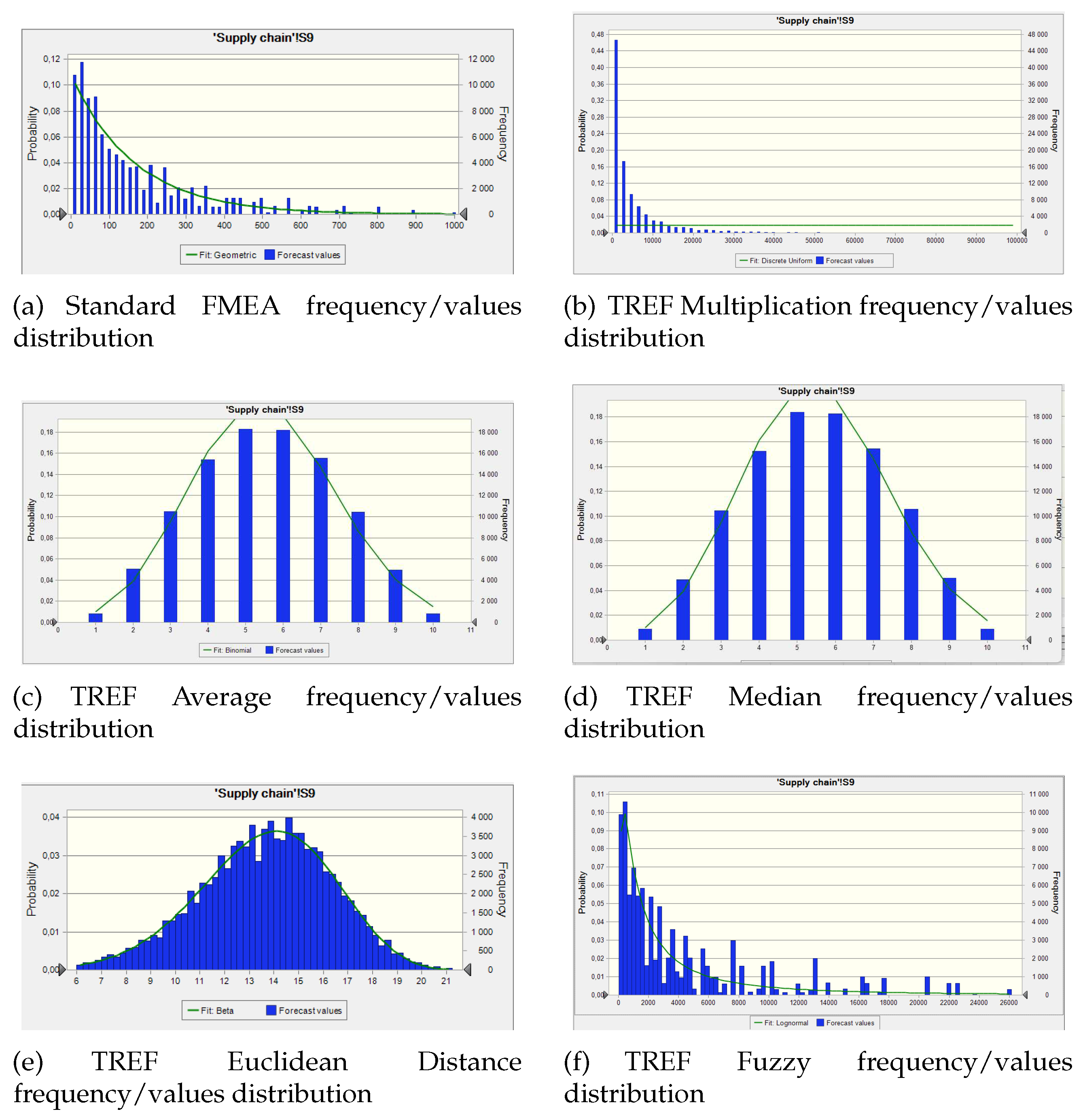
The utilization of the frequency perspective in the assessment process can prove to be useful. The Crystal Ball application developed by Oracle, which is an add-in for Microsoft Excel, was employed for this purpose. For the examination of three variables, specifically for the conventional FMEA, the trial number was established at 10,000. In this particular case, the sensitivity for each element was 33.3In the case of evaluating five factors, the trial numbers were set to 100,000 in order to achieve equal sensitivity for each element, with each factor accounting for 20% of the total.

Figure 5 displays the generated figures.

Table 4 presents a comprehensive overview of the simulations.

The Skewness in Table 4 pertains to the absence of symmetry in the dataset, whereas the Kurtosis assesses whether the data exhibit heavy (positive values) or light (negative values) tails relative to a normal distribution.

Upon examination of the simulation figure (Figure 5)), it is evident that:

The results obtained via the Multiplication Aggregation Method, as depicted in Figure 5.b, exhibit a level of comparability to those obtained from a conventional FMEA. However, it should be noted that the former method involved the consideration of five components, whereas the latter method typically considers three components. The linearity of the Multiplication technique and the standard FMEA is commendable. Consequently, the outcome for a scenario including n factors will yield a range of $[1, 10^{n}]$ for each factor, where the range of each factor is $[1, 10]$ . The concerns of FMEA are equally relevant in this particular case.
The input range and output range for the Average aggregate in Figure 5.c are identical, spanning from 1 to 10. Demonstrates strong linearity. The presence of extreme values can pose challenges in some scenarios. In the event that one factor attains its maximum value and the remaining factors maintain low values, the resulting output will nevertheless fall below the midpoint of the output range. In this particular scenario, the presence of low-value components effectively mitigates the impact of any extreme values, hence impeding the identification and analysis of potential risks.
The Median aggregation yields the lowest Skewness score, as depicted in Figure 5.d, suggesting that the data exhibits a high degree of symmetry. The Kurtosis score of our dataset is rather low, suggesting a moderate level of customization in the data. This situation bears resemblance to the Average aggregation approach.
The linearity is only average and the computation is challenging in the case of the Euclidean distance (generalized) aggregate (see Fig. Figure 5.e). Interpretation is challenging in n-dimensional space where n>3. In the case of n factors, the output will be $[1, 10 \sqrt{n}]$ for each factor’s range of values of $[1, 10]$ . The linearity of the Euclidean distance (generalized) aggregate is only average, and its computation is problematic, as depicted in Figure 5.e. The task of interpretation becomes complex when dealing with n-dimensional space, where n exceeds three. For a given number of factors, denoted as n, the resulting output will range from 1 to $10 \sqrt{n}$ . This range applies to each individual factor within the set of factors, where each component’s values vary from 1 to 10.
The outcome data for the Fuzzy aggregation method (refer to Figure 5.f), which is determined by the used membership and defuzzification functions, exhibit similarities to those of the TREF Multiplication. However, it is important to note that the output consists of just five primary groups (see Figure 1).

In conclusion, it is important to acknowledge that aggregations utilizing multiplication approaches, such as FMEA, generalized TREF Multiplication, and TREF Fuzzy with respect to defuzzification, yield the most unfavorable distribution. However, their significant contributions become essential in situations when elements exhibit elevated levels of risk.

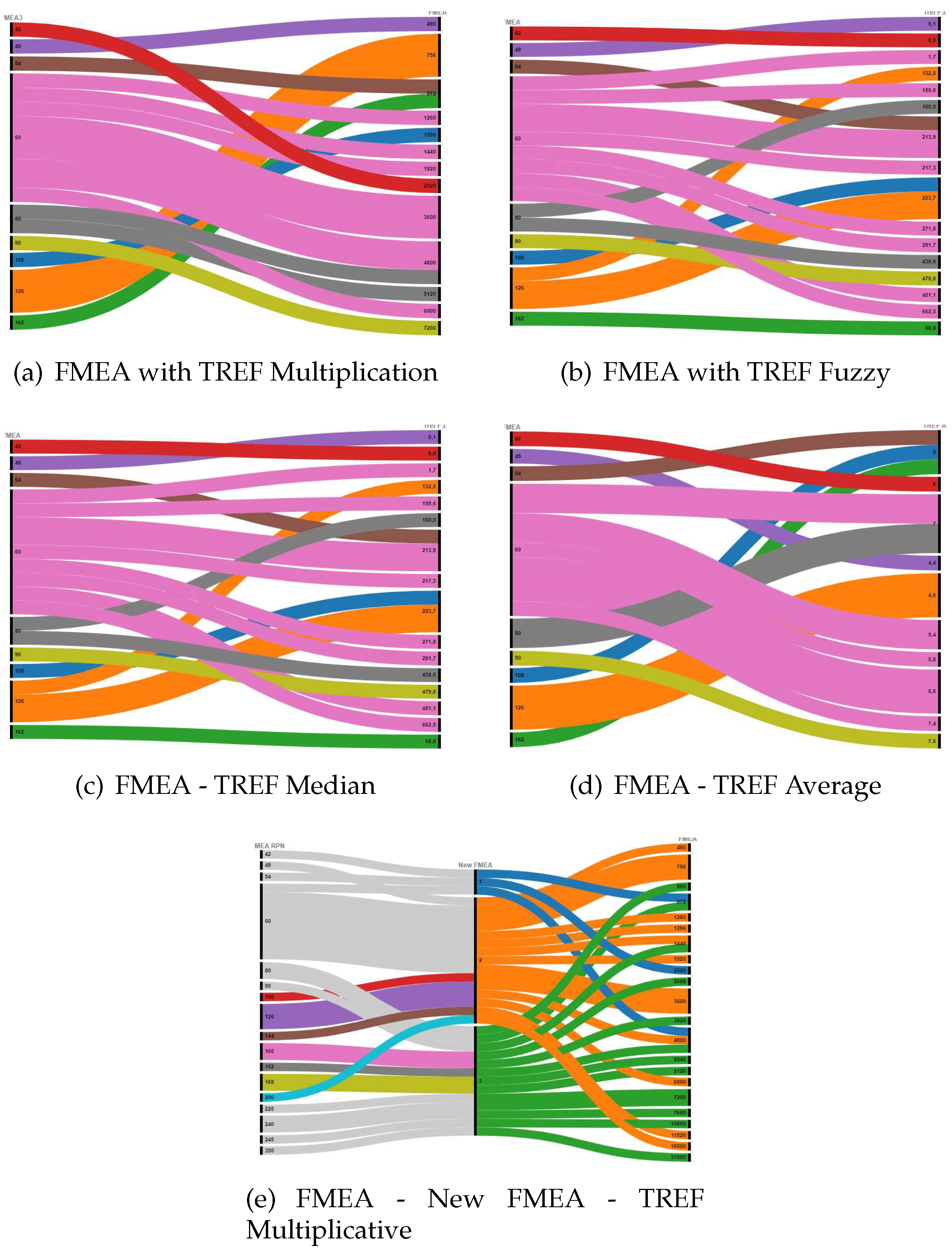
The reason for arranging each output in decreasing order was to ensure that this pattern was accurately represented. The comparative analysis of rank modifications for various aggregation functions is illustrated in Figure 6.

The present graphic depiction of Alluvian representation serves to emphasize the discrepancies in ordering through the comparison of an initial state and a subsequent state. The depiction, however, commences with the conventional outcomes of the FMEA as a foundation, considering the sequential Risk Priority Number (RPN) or output values. Subsequently, it demonstrates the alteration in prioritization of the aforementioned risk subsequent to the implementation of the novel aggregate function. The final diagram encompasses a triple figure that visually represents the transition from the conventional FMEA to the enhanced FMEA incorporating risk levels. This diagram enables readers to discern the differences between the two approaches. Additionally, the diagram includes the TREF Multiplicative, which functions as a comprehensive representation of various components. Please refer to Figure 6.e for further details.

The comparison between the conventional FMEA and the TREF Fuzzy method depicted in Figure 6.b holds significant importance in this study as it demonstrates the optimal results achieved by the utilization of the TREF Fuzzy aggregation function, as indicated in Table 3. The outcome was validated by the team of experts.

Outcome: The results obtained from this approach have been implemented, following the PDCA model (see Figure 4), and are presently under close scrutiny. If a new type of failure or unforeseen outcomes arise, the analysis will be repeated. After a period of six months of usage, no variation was seen.

Remark: The purpose of this paper is to provide a comprehensive guide for the identification of risks connected with Supply Chain Management (SCM). Its objective is to facilitate a thorough understanding of various risk variables and their corresponding significance. This document imposes some limitations, with the exception of donations. The process of prioritizing risks is contingent upon the thorough examination, evaluation, and distinctive perspectives that have surfaced pertaining to the manufacturing facility in question, and at the specific moment of the expert’s deliberation. Consequently, a hasty method has the potential to significantly undermine the precision and reliability of the investigation.

Acknowledgment

This work has been implemented by the TKP2021-NVA-10 project with the support provided by the Ministry of Culture and Innovation of Hungary from the National Research, Development and Innovation Fund, financed under the 2021 Thematic Excellence Programme funding scheme.

Abbreviations

The following abbreviations are used in this manuscript:

AP - Action Priority, the term used in the new

AHP - Analytical Hierarchy Process

ANP - Analytical Network Process

ERP - Enterprise Resource Planning

FMEA - Failure Mode and Effect Analysis

MFI - Mamdani Fuzzy Inference

OEM - Original Equipment Manufacturers, refers to the car companies in this article

QMS - Quality Management System (ISO9001, IATF16949, etc.)

PDCA - Plan, Do, Check, and Act - a the basis of any continuous improvement model

RPN - Risk Priority Number

SCM - Supply Chain Management

TOPSIS - Technique for Order Preference by Similarity to the Ideal Solution

TREF - Total Risk Evaluation Framework, is a generalized risk evaluation tool

Tier X - Suppliers in the automotive industry are organized in sequential levels called Tiers. The number X means how far are they from the OEM

Appendix A

Table A1. Criteria for evaluating the frequency of Occurrence of logistic defects at incoming

Probability of occurrence	Occurrence definition	Score
Never	Never	1
Unlikely	Once a year	2
Very low	Once a month	3
Low	Once a week	4
Medium	Once a day	5
Medium high	Daily 2-4 time	6
Important	Daily 5-10 time	7
Very important	Once in an hour	8
Very very important	Hourly 2-4 time	9
Extremely important	Hourly more than 6 time	10

Table A2. Criteria for evaluating the severity of the logistic failure defects

Severity of failure	Severity ranking	Score
No discernible effect	No discernible effect	1
Slight inconvenience in logistic process	Alarm at SCM	2
Can cause short stops	Red alarm at SCM	3
Can cause considerable stops in process	Can cause written remark	4
Small stops at Tier1	Warning from Tier1	5
Several small stops at Tier1	Escalation by Tier1	6
Serious stops at Tier1	Red alarm at Tier1	7
Delay at final customer	Escalation start from final customer	8
Small stops at final customer	Emergency at final customer	9
Serious stop at final customer	Stop final customer	10

Table A3. Criteria for assessing the detection of defects

Probability of detection	Detection effect	Score
Automatic detection	No effect	1
Extremely Easy detection	Easy to detect	2
Very high probability	Small delays	3
High probability	Detected delays	4
Medium	Late deliveries	5
Little	Several late deliveries	6
Very little	Line stops	7
Hard to detect	Several line stops	8
Extremely high	Customer stop	9
Undetectable	End customer stop	10

Table A4. Criteria for evaluating the cost of logistic defects

Probability of Cost	Cost definition	Score
Never	No cost	1
Very small	Non significant	2
Small	Tens of €	3
Low	Hundreds of €	4
Medium low	1-2k€	5
Medium	2-5k€	6
Significant	5-10k€	7
High	10-25k€	8
Very High	25-100k€	9
Extremely high	Over 100k€	10

Table A5. Criteria for evaluating the controllability of logistic defects

Probability of Control	Control definition	Score
Fully controlled	No	1
Very easy control	Needs small attention	2
Easy control	Attention	3
Gap in control	Easy re-planning	4
Several gaps in control	Re-planning	5
Serious gaps in control	Fast reaction	6
Difficult to control	Several fast reactions	7
Very difficult to control	Difficult	8
Partially out of control	Very difficult	9
Completely out of control	Impossible	10

Table A6. A detail from the standard and new FMEA analysis results - for 3 factors

No	Process	Sub-Process	Failure mode	Effect	O	S	D	RPN	AP
1	handling	at supplier	damaged	stop prod/cust	2	9	9	162	H
2	handling	during transp	damaged	stop prod/cust	2	9	7	126	M
3	handling	during uploading	damaged	stop prod/cust	2	9	7	126	M
4	handling	during downloading	damaged	stop prod/cust	2	9	7	126	M
5	handling	delay(nat.hol)	delay in production	stop cust or delay	1	7	7	49	M
6	transport	delay traffic	delay in production	stop cust or delay	1	9	6	54	M
7	transport	delay disaster	delay in production	stop cust or delay	1	10	6	60	M
8	transport	accident	delay in production	stop cust or delay	1	10	6	60	M
9	mat.ordering	order mistake	stop production	stop customer	1	10	6	60	M
10	IT system	IT failure	system error	stop customer	1	10	6	60	M
11	WH	mat.ordering	mat shortage at reseller or supply	stop customer	1	10	6	60	M
12	WH	mat.ordering	mat. shortage market situ	stop customer	1	10	6	60	M
13	WH	mat.ordering	distrib WH issue	stop customer	1	10	6	60	M

Table A7. Ranking of effect by experts from EMS company

No	C1	C2	C3	C4	C5	C6	C7	C8	C9	C10	C11	C12	C13	C14	C15	C16	C17	C18	C19	C20
C1	1	4.5	4	5	1	0.33	2	1	7.5	7	3	1.5	2.5	0.83	6	3.5	8.5	5.5	6.5	0.5
C2	0.22	1	0.83	1.2	0.25	0.17	0.33	0.25	3	2.5	0.5	0.33	0.5	0.2	1.5	0.67	4	2	2.5	0.25
C3	0.25	1.2	1	1.5	0.29	0.18	0.4	0.29	3.5	3	0.67	0.33	0.5	0.2	2	0.83	4.5	1.5	2.5	0.2
C4	0.2	0.83	0.67	1	0.22	0.15	0.4	0.29	3.5	3	0.67	0.33	0.5	0.2	2	0.83	4.5	1.5	2.5	0.2
5C	1	4	3.5	4.5	1	0.5	15	1.2	7	6.5	2.5	1	2	0.5	5.5	3	7.5	5	6	0.67
C6	3	6	5.5	6.5	2	1	3.5	2.5	9	8.5	4.5	3	4	1	7.5	5	9.5	7	8	1
C7	0.5	3	2.5	3	0.67	0.29	1	0.83	6.5	5	1.3	0.9	1.2	0.4	4	1.5	6.5	3.5	4.5	0.33
C8	1	4	3.5	4	0.83	0.4	1.2	1	6.5	6	2	1.2	1.5	0.67	5	2.5	7.5	4.5	5.5	0.5
C9	0.13	0.33	0.29	0.4	0.14	0.11	0.15	0.15	1	0.8	0.22	0.17	0.2	0.13	0.15	0.25	2	0.5	0.83	0.12
C10	0.14	0.4	0.33	0.5	0.15	0.12	0.2	0.17	1.25	1	0.25	0.18	0.22	0.13	0.83	0.29	3	0.67	0.91	0.13
C11	0.33	2	1.5	2	0.4	0.22	0.77	0.5	4.5	4	1	0.67	0.91	0.29	3	1.2	5	2.5	3.5	0.25
C12	0.67	3	3	3.5	1	0.33	1.11	0.83	6	5.5	1.5	1	1.2	0.5	0.22	2	6.5	4	5	0.4
C13	0.4	2	2	2.5	0.5	0.25	0.83	0.67	5	4.5	1.1	0.83	1	0.33	3.5	1.2	5.5	3	4	0.29
C14	1.2	5	5	5.5	2	1	2.5	1.5	8	7.5	3.5	2	3	1	6.5	4	8.5	6	7	0.83
C15	0.17	0.67	0.5	0.67	0.18	0.13	0.25	0.2	6.5	1.2	0.33	4.5	0.29	0.15	1	0.4	2	0.83	1.2	0.14
C16	0.29	1.5	1.2	1.5	0.33	0.2	0.67	0.4	4	3.5	0.83	0.5	0.83	0.25	2.5	1	5	2	3	0.22
C17	0.12	0.25	0.22	0.29	0.13	0.11	0.15	0.13	0.5	0.33	0.2	0.15	0.18	0.12	0.5	0.2	1	0.4	0.67	0.11
C18	0.18	0.5	0.67	0.77	0.2	0.14	0.29	0.22	2	1.5	0.4	0.25	0.33	0.17	1.2	0.5	2.5	1	1.2	0.15
C19	0.15	0.4	0.4	0.56	0.17	0.13	0.22	0.18	1.2	1.1	0.29	0.2	0.25	0.14	0.83	0.33	1.5	0.83	1	0.13
C20	2	4	5	6	1.57	1	3	2	8.5	8	4	2.5	3.5	1.2	7	4.5	9	6.5	7.5	1

A8:

Table A8. Random evaluation of impacts in all risk cases

No	C1	C2	C3	C4	C5	C6	C7	C8	C9	C10	C11	C12	C13	C14	C15	C16	C17	C18	C19	C20
Eval	+	-	+	-	+	-	+	-	+	-	+	-	+	-	+	-	+	-	+	-

A9:

Table A9. Evaluation of impacts in all risk cases based on ranking matrix

No	C1	C2	C3	C4	C5	C6	C7	C8	C9	C10	C11	C12	C13	C14	C15	C16	C17	C18	C19	C20
Eval	-	+	+	+	-	-	-	-	+	+	-	-	-	+	-	+	+	+	+	-

References

Huang, J.; You, J.X.; Liu, H.C.; Song, M.S. Failure mode and effect analysis improvement: A systematic literature review and future research agenda. Reliability Engineering & System Safety 2020, 199, 106885. [Google Scholar] [CrossRef]
AIAG-VDA. Failure Mode and Effects Analysis - FMEA Handbook; Vol. 1, Southfild, Michigan Automotive Industry Action Group [Berlin] [Verband der Automobilindustrie].
Dickson, W.G. An analysis of vendor selection systems and decisions. Journal of Purchasing 1966, 2, 5–20. [Google Scholar] [CrossRef]
Cheraghi, S.H.; Dadashzadeh, M.; Subramanian, M. Critical Success Factors For Supplier Selection: An Update. Journal of Applied Business Research (JABR) 2011, 20. [Google Scholar] [CrossRef]
Liu, H.C.; Liu, L.; Liu, N. Risk evaluation approaches in failure mode and effects analysis: A literature review. Expert Systems with Applications 2013, 40, 828–838. [Google Scholar] [CrossRef]
Sime Curkovic, Thomas Scannell, B.W. Using FMEA for Supply Chain Risk Management. Modern Management Science & Engineering 2013, 1, 251–256.
Wagner, S.C.T.S.B. ManagingSupply Chain Risk, Integrating with Risk Management; CRC Press, Taylor & Francis Group, LLC, 2016.
Vodenicharova, M. Opportunities for the applications of FMEA Model in logistics processes in Bulgarian enterprises. Logistics & Sustainable Transport 2017, 8, 31–41. [Google Scholar] [CrossRef]
Lolli, F.; Ishizaka, A.; Gamberini, R.; Rimini, B.; Messori, M. FlowSort-GDSS – A novel group multi-criteria decision support system for sorting problems with application to FMEA. Expert Systems with Applications 2015, 42, 6342–6349. [Google Scholar] [CrossRef]
Malekitabar, H.; Ardeshir, A.; Sebt, M.H.; Stouffs, R.; Teo, E.A.L. On the calculus of risk in construction projects: Contradictory theories and a rationalized approach. Safety Science 2018, 101, 72–85. [Google Scholar] [CrossRef]
Wu, X.; Wu, J. The Risk Priority Number Evaluation of FMEA Analysis Based on Random Uncertainty and Fuzzy Uncertainty. Complexity 2021, 2021, 1–15. [Google Scholar] [CrossRef]
Ewa Kulinska, D.M.; Dendera-Gruszka, M. New Application of FMEA Analysis in the Heavy Industry Supply Chain. techreport vol. XXIV, issue 2B, 600-616, European Research Studies Journal, 2021.
Ebadi, A.; Keyghobadi, A.R.; Motadel, M.R.; Yeganegi, M.R. The Analysis of Sustainable Supply Chain Risks Based on the FMEA Method in the Oil and Gas industry and Factors Affecting Risk Management. Petroleum Business Review 2020, 4. [Google Scholar] [CrossRef]
Indrasari, L.D.; Vitasmoro, P.; Pariyanto, A.Y.T. FMEA Approach to Risk Factors as a Factor in Implementing Green Supply Chain Management (Study in PT. Gresik Cipta Sejahtera). Journal of Physics: Conference Series 2021, 1858, 012069. [Google Scholar] [CrossRef]
Aleksic, B.; Djekic, I.; Miocinovic, J.; Memisi, N.; Smigic, N. Application of FMEA Analysis in the Short Cheese Supply Chain. Meat Technology 2020, 61, 161–173. [Google Scholar] [CrossRef]
Mustaniroh, S.A.; Murod, F.A.I.K.; Silalahi, R.L.R. The risk assessment analysis of corn chips supply chain using Fuzzy FMEA. IOP Conference Series: Earth and Environmental Science 2020, 475, 012052. [Google Scholar] [CrossRef]
Trenggonowati, D.L.; Bahauddin, A.; Ridwan, A.; Wulandari, Y. Proposed Action of Supply Chain Risk Mitigation Air Compressor Type L Unloading ¼ HP Using The Fuzzy – FMEA and Fuzzy – AHP Method in PT. XYZ. Journal of Innovation and Technology 2021, 2, 10–17. [Google Scholar] [CrossRef]
Lu Lu, R.Z.; de Souza, R. Enhanced FMEA for supply chain risk identification. The Road to a Digitalized Supply Chain Management: Smart and Digital Solutions for Supply Chain Management,; Hamburg University of Technology (TUHH), I.o.B.L.; Management, G., Eds. epubli, 2018, pp. 311–330. [CrossRef]
Petrović, D.V.; Tanasijević, M.; Milić, V.; Lilić, N.; Stojadinović, S.; Svrkota, I. Risk assessment model of mining equipment failure based on fuzzy logic. Expert Systems with Applications 2014, 41, 8157–8164. [Google Scholar] [CrossRef]
Trenggonowati, D.L.; Ulfah, M.; Arina, F.; Lutfiah, C. Analysis and strategy of supply chain risk mitigation using fuzzy failure mode and effect analysis (fuzzy fmea) and fuzzy analytical hierarchy process (fuzzy ahp). IOP Conference Series: Materials Science and Engineering 2020, 909, 012085. [Google Scholar] [CrossRef]
Canbakis, S.K.; Karabas, M.; Kilic, H.S.; Koseoglu, S.; Unal, E. A risk assessment model for supply chains. Pressacademia 2018, 7, 122–125. [Google Scholar] [CrossRef]
Zammori, F.; Gabbrielli, R. ANP/RPN: a multi criteria evaluation of the Risk Priority Number. Quality and Reliability Engineering International 2011, 28, 85–104. [Google Scholar] [CrossRef]
Ling, W.K. Nonlinear Digital Filters; Elsevier Ltd: Amsterdam Boston London, 2004.
Kubler, S.; Robert, J.; Derigent, W.; Voisin, A.; Traon, Y.L. A state-of the-art survey & testbed of fuzzy AHP (FAHP) applications. 65, 398–422. [CrossRef]
Johanyák, Z.; Kovács, S. On the right selection of the fuzzy membership function. GAMF Journal 2004, XIX, 73–84. [Google Scholar]
Zhu, Q.; Golrizgashti, S.; Sarkis, J. Product deletion and supply chain repercussions: risk management using FMEA. Benchmarking: An International Journal 2020, 28, 409–437. [Google Scholar] [CrossRef]
Wan, C.; Yan, X.; Zhang, D.; Qu, Z.; Yang, Z. An advanced fuzzy Bayesian-based FMEA approach for assessing maritime supply chain risks. Transportation Research Part E: Logistics and Transportation Review 2019, 125, 222–240. [Google Scholar] [CrossRef]
Dendera-Gruszka, M.; Kulińska, E. Supply Chain FMEA Risk Analysis for the Heavy Industry Sector. In Risk Management and Assessment; IntechOpen, 2020. [CrossRef]
Kosztyán, Z.T.; Csizmadia, T.; Kovács, Z.; Mihálcz, I. Total risk evaluation framework. International Journal of Quality & Reliability Management 2020, 37, 575–608. [Google Scholar] [CrossRef]
Kovács, Z.; Kosztyán, Z.T.; Csizmadia, T. TREF – Total Risk Evaluation Framework: integrált kockázatmenedzsment-szemléletu keretrendszer kifejlesztése és bevezetése egy magyarországi termelovállalatnál. Vezetéstudomány / Budapest Management Review 2014, pp. 71–82. [CrossRef]
Kovács, Z.; Csizmadia, T.; Mihálcz, I.; Kosztyán, Z.T. A vállalati kockázatkezelésben használt aggregálófüggvények jellemzése. 100, 821–853. [CrossRef]
Calvo, T.; Kolesárová, A.; Komorníková, M.; Mesiar, R. Aggregation Operators: Properties, Classes and Construction Methods. In Aggregation Operators; Physica-Verlag HD, 2002; pp. 3–104. [CrossRef]
Grabisch, M.; Marichal, J.L.; Mesiar, R.; Pap, E. Aggregation functions: means. Information Sciences 2011, 181, 1–22. [Google Scholar] [CrossRef]
Kozarević, S.; Puška, A. Use of fuzzy logic for measuring practices and performances of supply chain. 5, 150–160. [CrossRef]
Cardiel-Ortega, J.J.; Baeza-Serrato, R. Failure Mode and Effect Analysis with a Fuzzy Logic Approach. 11, 348. [CrossRef]
Chakraborty, S. TOPSIS and Modified TOPSIS: A comparative analysis. 2, 100021. [CrossRef]
Bognár, F.; Hegedus, C. Analysis and Consequences on Some Aggregation Functions of PRISM (Partial Risk Map) Risk Assessment Method. 10, 676. [CrossRef]
Yazdi, M.M. TOPSIS method for multiple-criteria decision making (MCDM).

Figure 1. The structure of Fuzzy membership functions for each factor.

Figure 2. Used DeFuzzyfication methods to obtain the final output value.

Figure 3. The supply chain map of the EMS company.

Figure 4. Determination of the appropriate risk evaluation method

Figure 5. Results - Frequency

Figure 6. Results - Alluvian representation of original FMEA ranking with the used 5 TREF functions

Table 1. A detail from the ranking matrix composed from the standard FMEA, TREF Multiplicative, Tref Average, TREF Median, TREF Distance, and TREF Fuzzy functions - the last 5 evaluations were made using 5 factors.

No	R. FMEA	R. TREF Multi	R. TREF Aver	R. TREF Medi	R. TREF Dist	R. TREF Fuzzy
1	1	15	15	17	14	17
2	2	17	17	18	17	8
3	3	18	18	19	18	9
4	5	13	14	14	16	7
5	4	19	19	20	19	16
6	19	20	20	16	20	20
7	18	16	16	15	15	13
8	9	7	7	7	7	15
9	10	5	5	5	4	2
10	6	1	1	2	1	3
11	11	6	6	6	5	11
12	7	3	3	3	6	14
13	12	14	13	13	12	12

Table 2. Ranking of methods using TOPSIS without considering the weights

Alt. row	Name	Score	Rank
1	FMEA	0.6308374	1
2	TREF Multi	0.4312619	4
3	TREF Aver	0.4338759	3
4	TREF Medi	0.4414542	2
5	TREF Dist	0.4132224	5
6	TREF FMEA	0.2516496	6

Table 3. Ranking of methods using TOPSIS with weights

Alt. row	Name	Score	Rank
1	FMEA	0.5959322	1
2	TREF Multi	0.5529383	3
3	TREF Aver	0.5538219	2
4	TREF Medi	0.5418204	4
5	TREF Dist	0.5364203	5
6	TREF FMEA	0.1567300	6

Table 4. Characteristics of different aggregation methods for 5 factors including the standard FMEA with 3 factors.

Item	FMEA	TREF Multi	TREF Aver	TREF Median	TREF EucDist	TREF Fuzzy
Factors	3	5	5	5	5	5
Skewness	1.66	3.34	-.0025	-.003	-.32	3.28
Kurtosis	5.77	18.84	2.36	2.37	3.02	17.91
Min	1	1	1	1	2	8
Max	1000	100000	10	10	22	77348

Disclaimer/Publisher’s Note: The statements, opinions and data contained in all publications are solely those of the individual author(s) and contributor(s) and not of MDPI and/or the editor(s). MDPI and/or the editor(s) disclaim responsibility for any injury to people or property resulting from any ideas, methods, instructions or products referred to in the content.

© 2023 by the authors. Licensee MDPI, Basel, Switzerland. This article is an open access article distributed under the terms and conditions of the Creative Commons Attribution (CC BY) license (http://creativecommons.org/licenses/by/4.0/).

Copyright: This open access article is published under a Creative Commons CC BY 4.0 license, which permit the free download, distribution, and reuse, provided that the author and preprint are cited in any reuse.

MDPI Initiatives

Important Links

Choose an area of interest and we will send you notifications of new preprints at your preferred frequency.

Disclaimer

No	R. FMEA	R. TREF Multi	R. TREF Aver	R. TREF Medi	R. TREF Dist	R. TREF Fuzzy
1	1	15	15	17	14	17
2	2	17	17	18	17	8
3	3	18	18	19	18	9
4	5	13	14	14	16	7
5	4	19	19	20	19	16
6	19	20	20	16	20	20
7	18	16	16	15	15	13
8	9	7	7	7	7	15
9	10	5	5	5	4	2
10	6	1	1	2	1	3
11	11	6	6	6	5	11
12	7	3	3	3	6	14
13	12	14	13	13	12	12

No	R. FMEA	R. TREF Multi	R. TREF Aver	R. TREF Medi	R. TREF Dist	R. TREF Fuzzy
1	1	15	15	17	14	17
2	2	17	17	18	17	8
3	3	18	18	19	18	9
4	5	13	14	14	16	7
5	4	19	19	20	19	16
6	19	20	20	16	20	20
7	18	16	16	15	15	13
8	9	7	7	7	7	15
9	10	5	5	5	4	2
10	6	1	1	2	1	3
11	11	6	6	6	5	11
12	7	3	3	3	6	14
13	12	14	13	13	12	12

REFS - A Risk Evaluation Framework on Supply Chain

Abstract

1. Introduction

2. Mathematical background

2.1. Aggregation functions criteria

2.2. Risk aggregation functions

2.3. Implementation of Fuzzy

2.3.1. Fuzzyfication/Fuzzyfier

2.3.2. Fuzzy rule base

2.3.3. Defuzzyfication

2.4. Rank correlation

2.5. TOPSIS (Technique for Order Preference by Similarity to Ideal Solution)

3. Case study

4. Discussion and Result

Acknowledgment

Abbreviations

Appendix A

References

MDPI Initiatives

Important Links

Subscribe

No	R. FMEA	R. TREF Multi	R. TREF Aver	R. TREF Medi	R. TREF Dist	R. TREF Fuzzy
1	1	15	15	17	14	17
2	2	17	17	18	17	8
3	3	18	18	19	18	9
4	5	13	14	14	16	7
5	4	19	19	20	19	16
6	19	20	20	16	20	20
7	18	16	16	15	15	13
8	9	7	7	7	7	15
9	10	5	5	5	4	2
10	6	1	1	2	1	3
11	11	6	6	6	5	11
12	7	3	3	3	6	14
13	12	14	13	13	12	12