Submitted:
13 December 2023
Posted:
15 December 2023
You are already at the latest version
Abstract
Keywords:
1. Introduction
2. Loss parallel system without queue
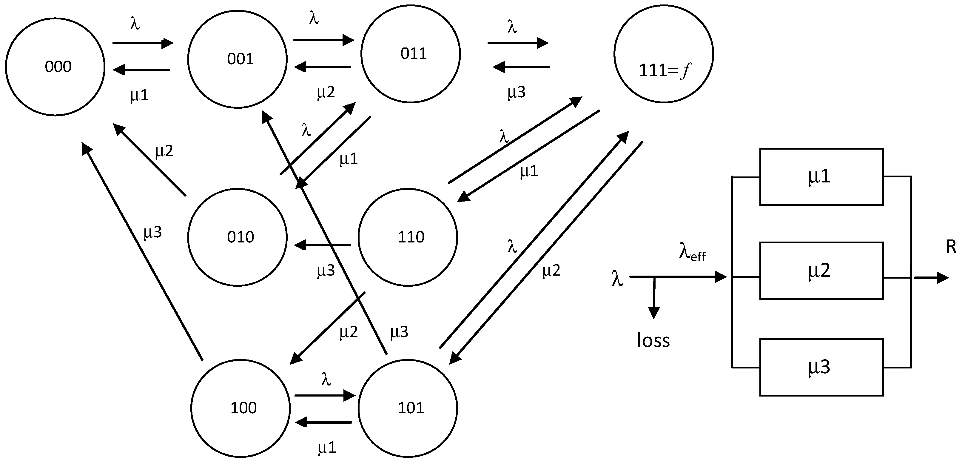
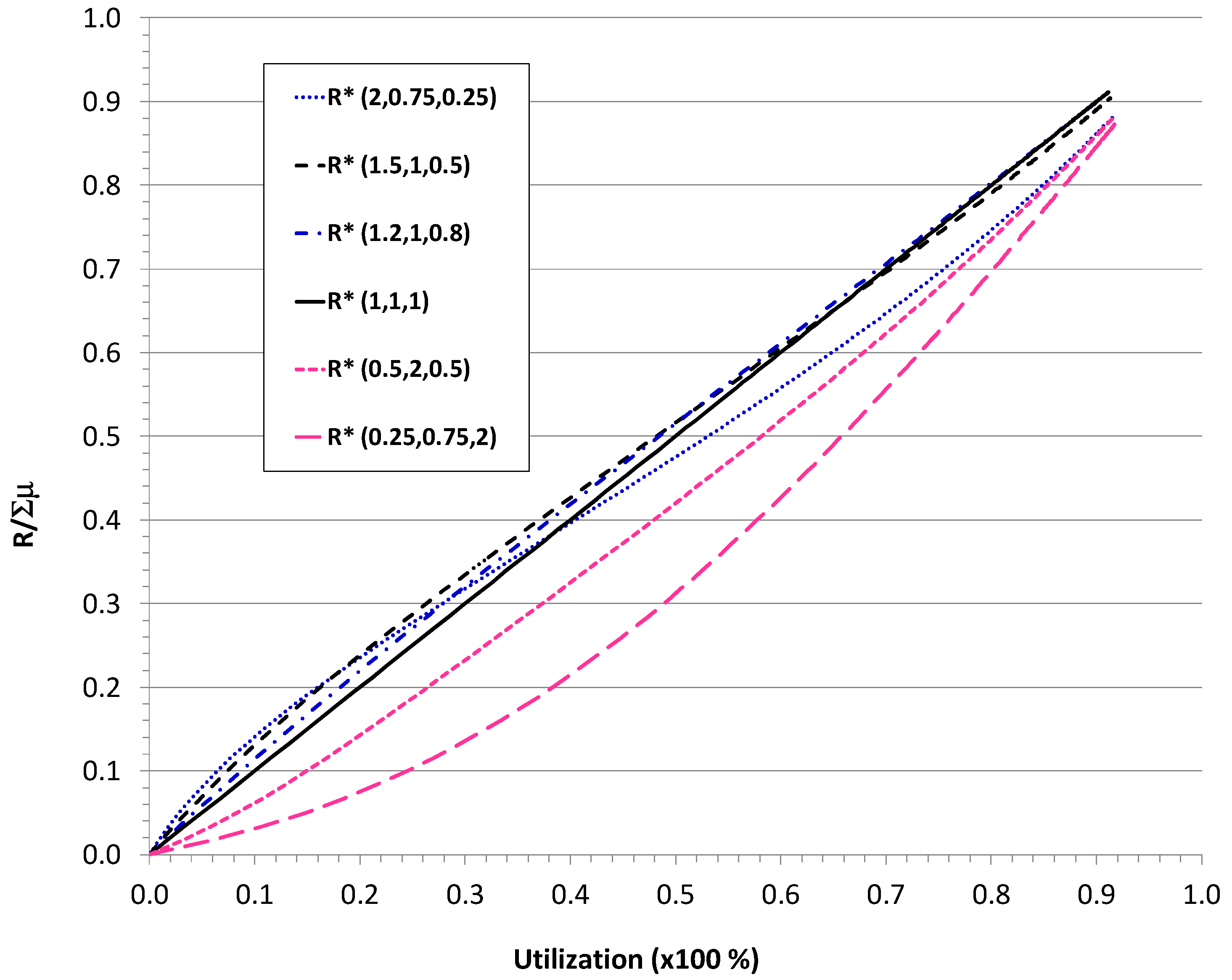
2.2. System of heterogeneous parallel servers
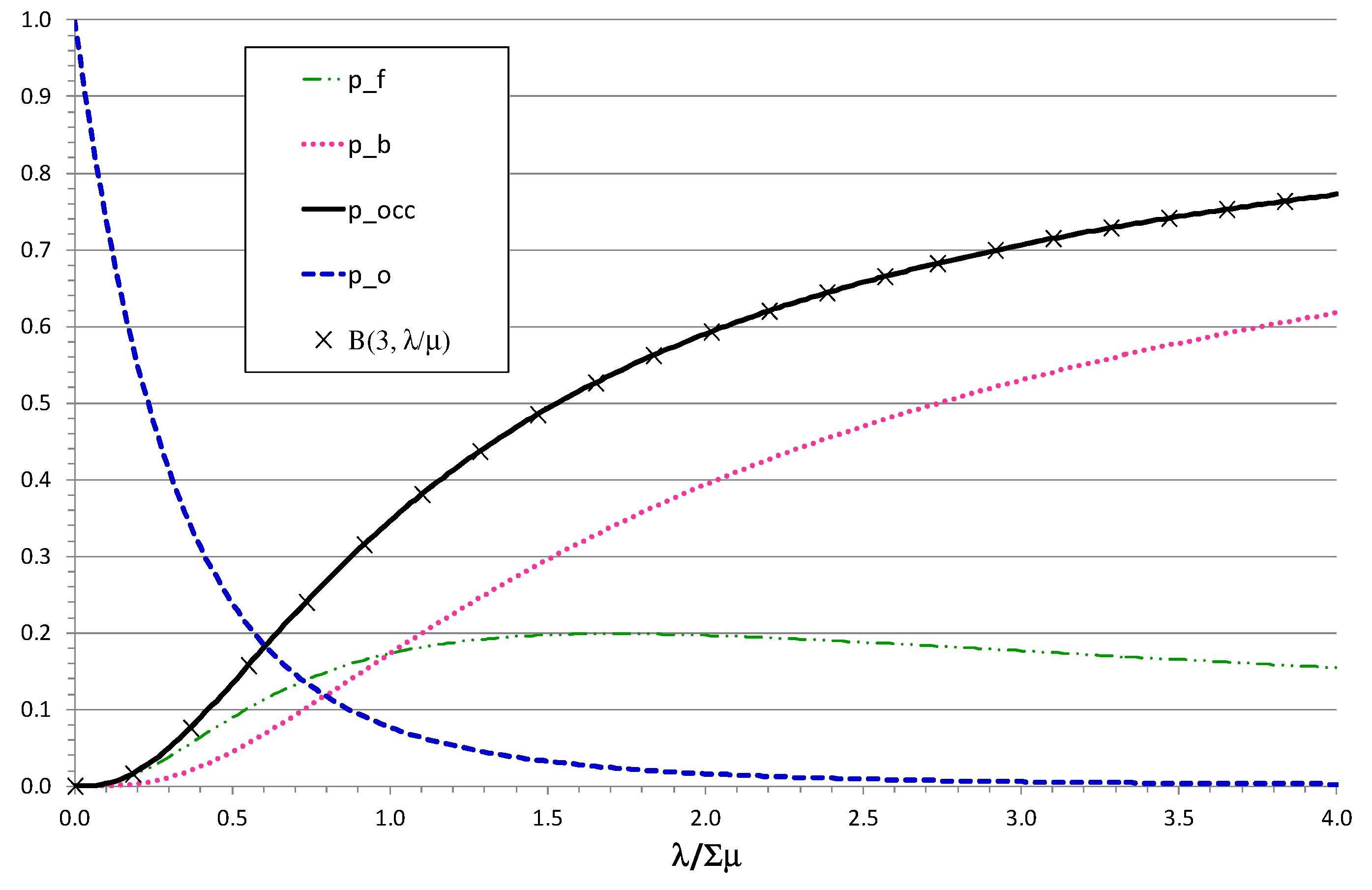
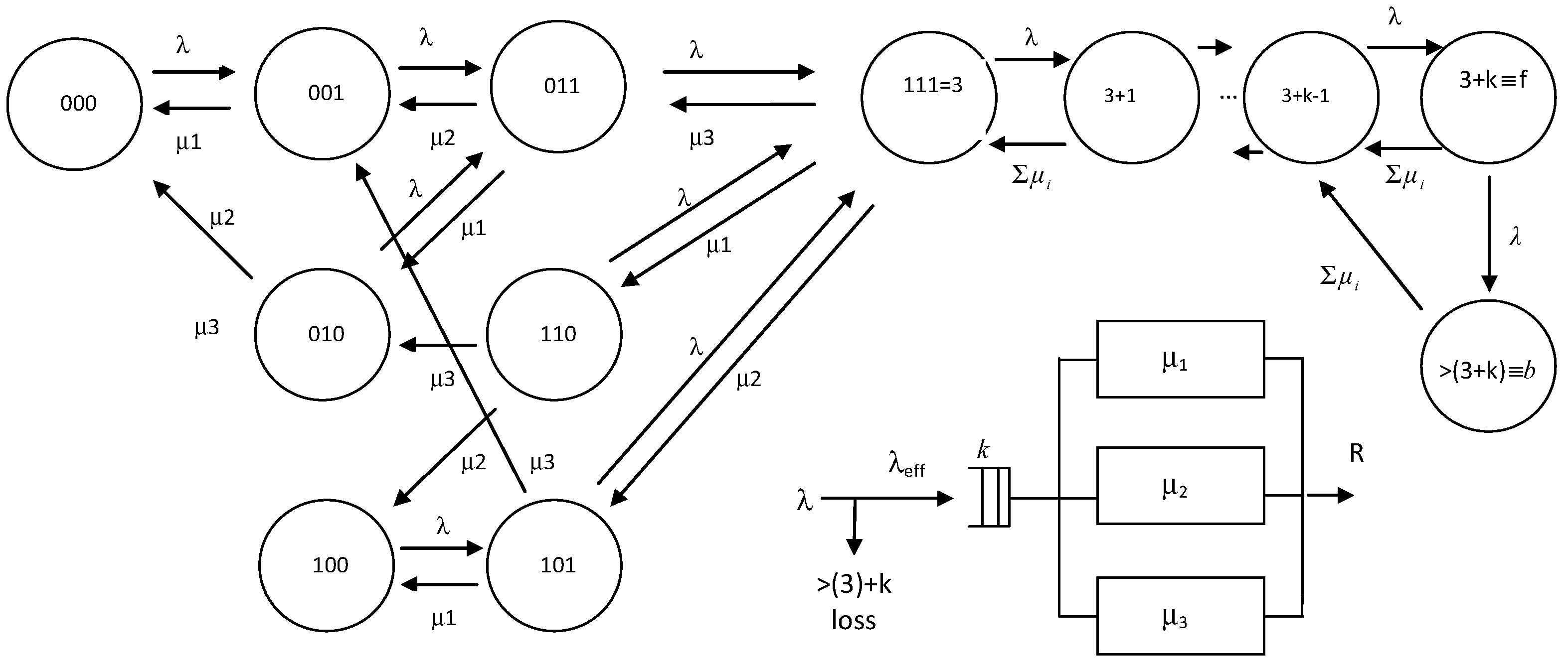
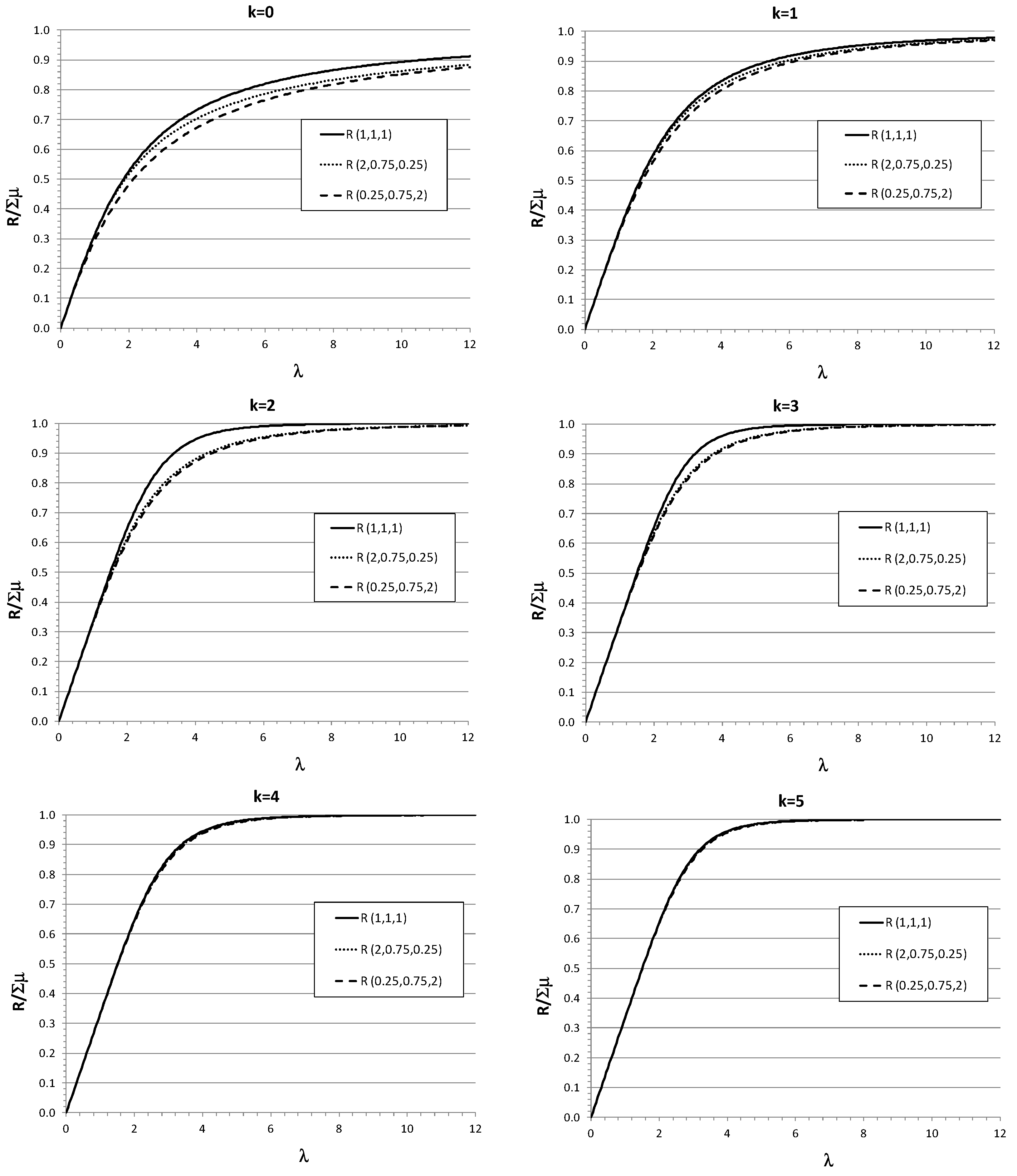
3. Parallel heterogeneous servers with a common waiting queue.
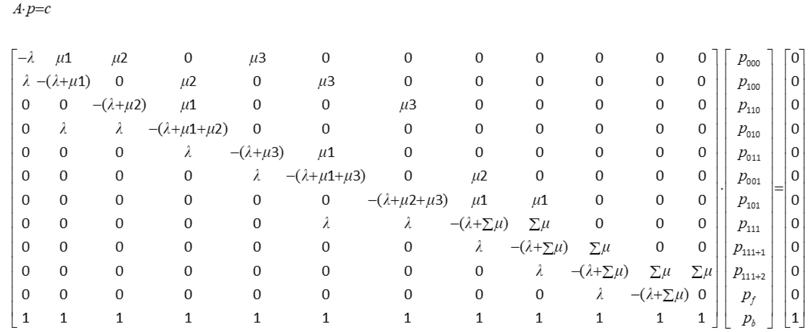
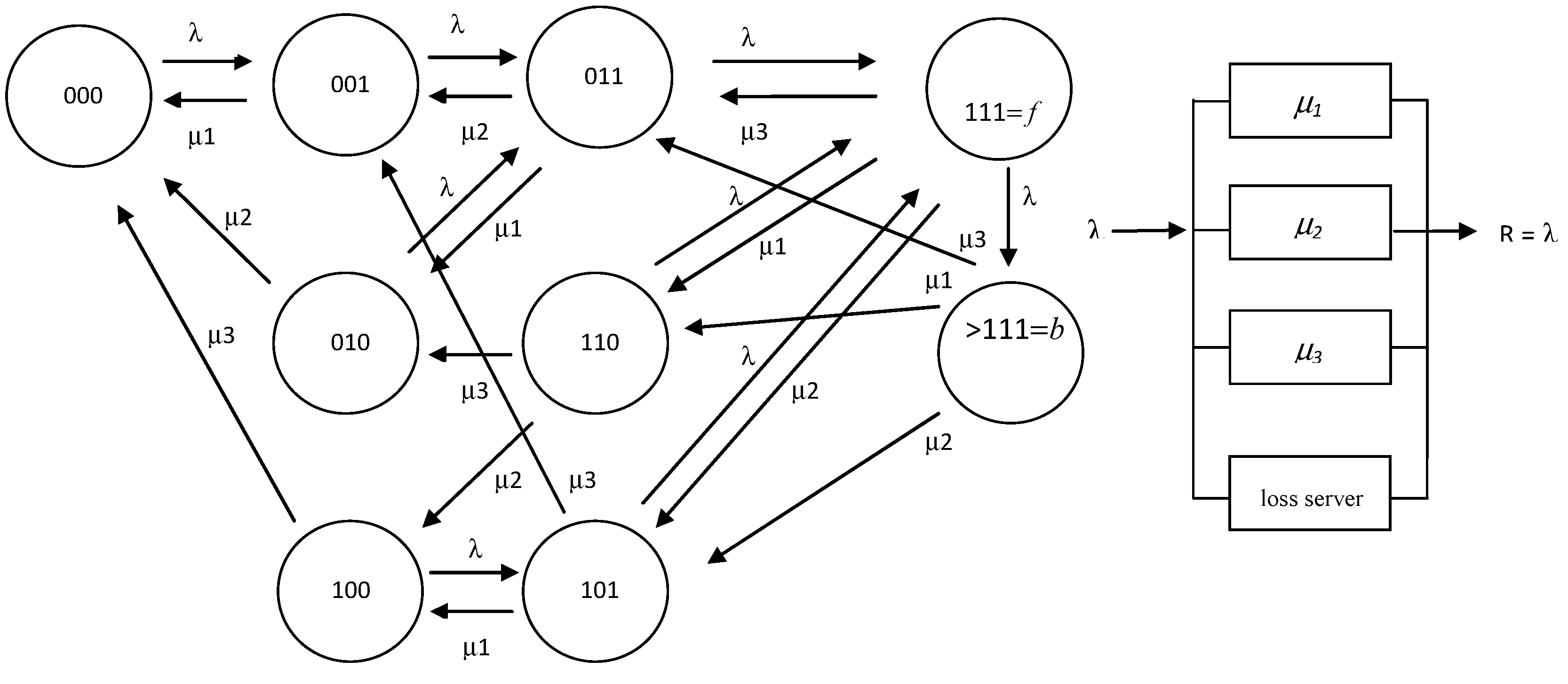
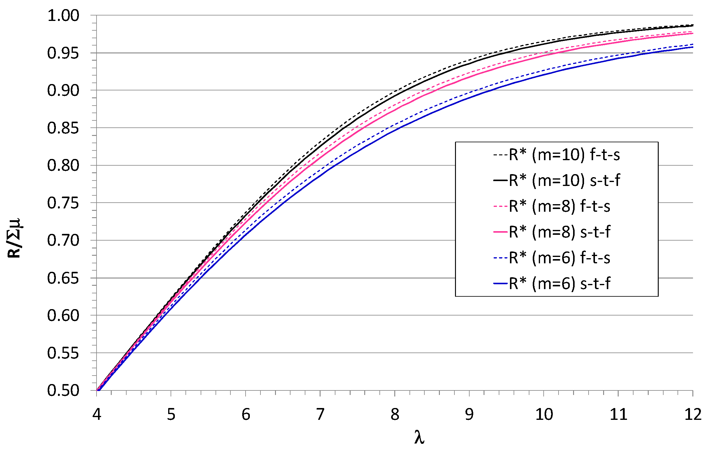
4. Parallel heterogeneous servers with a common waiting queue.
5. Hybrid modeling of heterogeneous servers with general service time distributions.
5.1. Uncertainty of the offered load
5.2. Application to non-exponential service time distributions
6. Conclusions
Author Contributions
Funding
Data Availability Statement
Conflicts of Interest
References
- Curry:, G.L.; Feldman, R.M. Manufacturing systems modelling and analysis; Springer Science & Business Media, 2010. [Google Scholar]
- Smith, J.M. Introduction to Queuing Networks: Theory ∩ Practice. Springer, 2018.
- Shortle, J.F.; Thompson, J.M.; Gross, D.; Harris, C.M. Fundamentals of queueing theory. John Wiley & Sons, 2018.
- Efrosinin, D. Controlled queueing systems with heterogeneous servers. 2004. https://d-nb.info/971824401/34.
- Wolff, R.W. Poisson arrivals see time averages. Operations Research 1982, 30, 223–231. [Google Scholar] [CrossRef]
- Gans, N.; Koole, D.; Mandelbaum, A. Telephone call centers: Tutorial, review, and research prospects. Manufacturing Service Operations Management 2003, 5, 79–141. [Google Scholar] [CrossRef]
- Armony, M.; Ward, A.R. Fair dynamic routing in large-scale heterogeneous-server systems. Operations Research 2010, 58, 624–637. [Google Scholar] [CrossRef]
- Gumbel, H. Waiting lines with heterogeneous servers. Operations Research 1960, 8, 504–511. [Google Scholar] [CrossRef]
- Disney, R.L. Some multichannel queueing problems with ordered entry. Journal of Industrial Enginering 1962, 13, 46–48. [Google Scholar]
- Disney, R.L. Some Multichannel Queueing Problems with Ordered Entry-an Application to Conveyor Theory. Journal of Industrial Engineering 1963, 14, 105–108. [Google Scholar]
- Singh, W.S. Two-server Markovian queues with balking: Heterogeneous vs. homogeneous servers. Operations Research 1970, 18, 145–159. [Google Scholar] [CrossRef]
- Singh, V.S. Markovian queues with three heterogeneous servers. IIE Transactions 1971, 3, 45–48. [Google Scholar] [CrossRef]
- Elsayed, E.A. Multichannel queueing systems with ordered entry and finite source. Computers & Operations Research 1983, 10, 213–222. [Google Scholar] [CrossRef]
- Yao, D.D. . The arrangement of servers in an ordered-entry system. Operations Research 1987, 35, 759–763. [Google Scholar] [CrossRef]
- Yao, D.A. Convexity properties of the overflow in an ordered-entry system with heterogeneous servers. Operations Research Letters 1986, 5, 145–147. [Google Scholar] [CrossRef]
- Saglam, V.; Shahbazov, A. Minimizing loss probability in queuing systems with heterogeneous servers. Iranian Journal of Science and Technology, Transaction A, Science 2007, 31, 199–206. [Google Scholar]
- Boxma, O.J.; Koole, G.M.; Liu, Z. Queueing-theoretic solution methods for models of parallel and distributed systems. Centrum voor Wiskunde in Informatica, Department of Operations Research, Statistics, and System Theory. 1994. https://ir.cwi.nl/pub/5133.
- Isguder, H.O.; Uzunoglu-Kocer, U. Analysis of GI/M/n/n queueing system with ordered entry and no waiting line. Applied Mathematical Modelling 2014, 38, 1024–1032. [Google Scholar] [CrossRef]
- Melikov, A.Z.; Ponomarenko, L.A.; Mekhbaliyeva, E.V. Analyzing the models of systems with heterogeneous servers. Cybernetics and Systems Analysis 2020, 56, 89–99. [Google Scholar] [CrossRef]
- Cooper, R.B. Queues with ordered servers that work at different rates. Operations Research, 1976; 13, 69–78. [Google Scholar] [CrossRef]
- Matsui, M.; Fukuta, J. On a Multichannel Queueing System with Ordered Entry and Heterogeneous Servers. AIIE Transactions 1977, 9, 209–214. [Google Scholar] [CrossRef]
- Nath, G.B.; Enns, E.G. Optimal service rates in the multiserver loss system with heterogeneous servers. Journal of Applied Probability 1981, 18, 776–781. [Google Scholar] [CrossRef]
- Pourbabai, B.; Sonderman, D. Service utilization factors in queueing loss systems with ordered entry and heterogeneous servers. Journal of Applied Probability 1986, 23, 236–242. [Google Scholar] [CrossRef]
- Muth, E.J.; White, J.A. Conveyor theory: A survey. AIIE Transactions 1979, 11, 270–277. [Google Scholar] [CrossRef]
- Nazzal, D.; El-Nashar, A. Winter Simulation Conference - Survey of research in modeling conveyor-based automated material handling systems in wafer fabs 2007, 1781–1788. [CrossRef]
- Nawijn, W.M. A note on many-server queueing systems with ordered entry, with an application to conveyor theory. Journal of Applied Probability 1983, 20, 144–152. [Google Scholar] [CrossRef]
- Nawijn, W.M. On a two-server finite queuing system with ordered entry and deterministic arrivals. European Journal of Operations Research 1984, 18, 388–395. [Google Scholar] [CrossRef]
- Pourbabai, B. Markovian queueing systems with retrials and heterogeneous servers. Computers and Mathematics with Applications 1987, 13, 917–923. [Google Scholar] [CrossRef]
- Boysen, N.; Briskorn, D.; Fedtke, S.; Schmickerath, M. Automated sortation conveyors: A survey from an operational research perspective. European Journal of Operations Research 2019, 276, 796–815. [Google Scholar] [CrossRef]
- Sonderman, D. An analytical model for recirculating conveyors with stochastic inputs and outputs. International Journal of Production Research 1982, 20, 591–605. [Google Scholar] [CrossRef]
- Schmidt, L.C.; Jackman, J. Modeling recirculating conveyors with blocking. European Journal of Operations Research 2000, 124, 422–436. [Google Scholar] [CrossRef]
- Brandwajn, A.; Jow, Y. An approximation method for tandem queues with blocking. Operations Research 1988, 36, 73–83. [Google Scholar] [CrossRef]
- Hsieh, Y.J. Analytical modeling of closed-loop conveyors with load recirculation. In: International Conference on Computational Science and Its Applications. Springer, Berlin, Heidelberg, 2005. [CrossRef]
- Haghighi, A.M.; Mishev, D.P. A parallel priority queueing system with finite buffers. Journal of Parallel Distributed Computing 2006, 66, 379–392. [Google Scholar] [CrossRef]
- Van der Gaast, J.P.; De Koster, M.B.M.; Adan, I.J. Conveyor merges in zone picking systems: A tractable and accurate approximate model. Transportation Science 2018, 52, 1428–1443. [Google Scholar] [CrossRef]
- Burke, P.J. The output of a queuing system. Operations Research 1956, 4, 699–704. [Google Scholar] [CrossRef]
- Armony, M. Dynamic routing in large-scale service systems with heterogeneous servers. Queueing Systems 2005, 51, 287–329. [Google Scholar] [CrossRef]
- Pike, R.; Martin, G.E. The bowl phenomenon in unpaced lines. International Journal of Production Research 1994, 32, 483–499. [Google Scholar] [CrossRef]
- Bolotin, V. Telephone circuit holding time distributions. In: Proc. 14th International Teletraffic Congress. The fundamental role of teletraffic in the evolution of telecommunications networks, Labetoulle, J. and Roberts, J.W.(Ed). Elsevier, 2014.

 |
 |
 |
 |
 |
Disclaimer/Publisher’s Note: The statements, opinions and data contained in all publications are solely those of the individual author(s) and contributor(s) and not of MDPI and/or the editor(s). MDPI and/or the editor(s) disclaim responsibility for any injury to people or property resulting from any ideas, methods, instructions or products referred to in the content. |
© 2023 by the authors. Licensee MDPI, Basel, Switzerland. This article is an open access article distributed under the terms and conditions of the Creative Commons Attribution (CC BY) license (http://creativecommons.org/licenses/by/4.0/).


