Fractional Order Mathematical Modelling of HFMD Transmission via Caputo Derivative

In this paper, we propose to explore a nonlinear fractional mathematical model of HFMD- Hand Foot Mouth Disease with vaccinated compartment. Firstly, we prove the non negativity and boundedness for the fractional order dynamical model. The system’s existence and uniqueness are studied using the formulation of the Caputo derivative operator. The fixed-point approach was used to get results indicating the presence of at least one solution. In numerical simulation, we obtained the approximate solution by using fractional Euler method.

Keywords:

Subject: Computer Science and Mathematics - Applied Mathematics

1. Introduction

Mathematical modeling involves using equations or algorithms to represent real-world systems across various disciplines such as physics, engineering, biology, economics, and social sciences. These models serve to comprehend, evaluate, and predict system behavior, playing a vital role in scientific research, engineering design, and decision-making. Mathematical modeling allows the study and control of systems in ways often impractical or costly in real-world experiments. The process typically includes problem formulation, model construction, parameter estimation, model validation, and model analysis. Proficiency in both system understanding and mathematics is crucial for creating and solving these equations. Validation and verification of models are essential before using them for predictions or decision-making. This interdisciplinary field combines mathematical concepts with domain-specific knowledge, providing insightful analyses of complex phenomena. Mathematical modeling is indispensable for advancing scientific understanding, addressing real-world issues, and making well-informed decisions. Researchers, engineers, and decision-makers leverage mathematical modeling to gain knowledge, predict outcomes, and optimize systems, contributing significantly to various fields [1,2,3,4].

The viral illness known as hand, foot, and mouth disease (HFMD) predominantly affects children under the age of ten and occasionally even adults. There are several enterovirus types that cause it, but Coxsackievirus A16 and Enterovirus 71 are the most frequent ones. The manifestation of diminutive and distressing blisters or ulcers on the hands, feet, and oral cavity, coupled with other indicators like fever and rash, typically points to the likelihood of Hand, Foot, and Mouth Disease (HFMD). It is highly contagious and spreads through close contact with infected individuals, contaminated surfaces, or respiratory droplets from coughs and sneezes. It is most commonly found in crowded places such as day care centres, schools, and playgrounds, and outbreaks often occur in communities, especially during the warmer months. The symptoms of HFMD usually start with fever, sore throat, and a general feeling of malaise. Within a day or two, small blisters will develop in the hands, feet and mouth. These blisters may be painful and can sometimes become ulcers. Other symptoms may include loss of appetite, headache, and in some cases, a skin rash. Although HFMD is often a temporary disease that cure by itself within seven to ten days, it can cause discomfort and sometimes complications, especially in severe cases. Complications can include viral meningitis, encephalitis (inflammation of the brain), and in rare cases, more serious neurological complications. Treatment for HFMD is usually supportive, focusing on relieving symptoms such as fever and discomfort. To manage discomfort and lower fever, over-the-counter pain medicines such as acetaminophen or ibuprofen may be used, and maintaining excellent hygiene habits, such as frequent handwashing and avoiding close contact with sick persons, is essential for preventing the virus’s spread. The important prevention is to maintain good oral hygiene and minimising contact with ill peoples. Vaccines for HFMD are not widely available, but some countries have developed vaccines against Enterovirus 71, which is one of the common causes of severe HFMD cases. Some recent research are presented in [5,6,7].

Fractional differential equations (FDEs) are differential equations that incorporate non-integer order derivatives. This permit the use of fractional orders, which can be any real or complex number, in contrast to ordinary differential equations (ODEs), where the order of the derivatives is always a positive integer [8]. When a system’s behaviour depends on the fractional derivatives of its variables, FDEs are an effective mathematical tool for describing a wide range of physical, biological, and engineering phenomena. In 18th and 19th centuries, mathematicians especially Leibniz and Riemann established the concept of fractional calculus, that is associated with non-integer order derivatives and integrals. However, because of its applications in numerous disciplines, including physics, engineering, finance, and biology, it has recently attracted new interest. Among other complex phenomena, FDEs have been used to model and examine viscoelastic materials, diffusion in fractal media, electrochemical processes, and biological systems. Most of the models stated above are integer order models, however they are unable to depict real life difficulties because there is no non-locality impact in local differentiation. Mathematicians thus developed the idea of differentiation with non-local operators to address this issue. The memory effect of fractional calculus has been demonstrated to produce more accurate results when predicting physical systems, including mathematical models [9]. In order to solve systems of differential equations of both integer and non-integer orders resulting from real life issues, such as applications related to integrodifferential equations, [10,11], mathematical epidemiology [12,13], economic and financial [14,15], new discoveries have resulted from advances in constructing new fractional order operators, especially Caputo, Atangana-Baleanu and Caputo-Fabrizio. Most researchers are optimistic on the fractional-order differential equation, especially in biological modelling [16]. A unique interpretation of the fractional operator without a single kernel was proposed by Caputo and Fabrizio [17]. In this paper, we choose Hand foot mouth disease as our social problem and formulated a five compartmental nonlinear mathematical model. Further, we extend the nonlinear ODE model into fractional order model by using Caputo derivative.

An overview of our article is provided below. In Section 2, the fractional order model was formulated, followed by some essential preliminaries in Section 3. In Section 4, we addressed the system’s positivity and boundedness. Section 5 discusses the suggested model’s existence and uniqueness, followed by the qualitative analysis in Section 6. The 7th section explains how to use the modified Euler’s approach to get the general solution to the suggested system. In Section 8, a brief summary was presented.

2. Model Formulation

We consider a

S V E I R

, five compartment HFMD model. The basic structure of the model comprises distinct population groups, including those that are susceptible, vaccinated, exposed, infected and recovered. In this case, we presume that not all vaccinated persons are immune to this virus, and that some may be exposed to it. We also believe that persons who have recovered from HFMD do not have a lifetime immunity to the condition. As a result, we believe that recovered people are susceptible at a rate of

α_{0}

, and that after recovery, some people will take vaccination and therefore enter the vaccinated compartment at a rate of

α_{1}

. As a result of the aforesaid assumptions, a basic nonlinear mathematical model was developed in [21]. That is,

\begin{matrix} \frac{d S}{d t} & = A - δ_{1} S I - δ_{2} S E - μ S - z S + α_{0} R, \\ \frac{d V}{d t} & = z S - δ_{3} V I - δ_{4} V E - μ V + α_{1} R, \\ \frac{d E}{d t} & = δ_{1} S I + δ_{2} S E + δ_{3} V I + δ_{4} V E - η E - μ E, \\ \frac{d I}{d t} & = η E - γ I - μ I - μ_{1} I, \\ \frac{d R}{d t} & = γ I - μ R - α_{0} R - α_{1} R . \end{matrix}

(1)

It is vital to investigate viral disease mathematical models in order to have a deeper comprehension of their assessment, presence, stability, and control. Because typical mathematical models do not provide a great level of precision in describing these diseases, FDE which have many uses in practical domains, were designed to manage such situations. So, here ODE model for HFMD in [21] was extended to the fractional order model by using the Caputo derivative.

\begin{matrix} ^{C} D_{t}^{α} [S (t)] & = A - δ_{1} S I - δ_{2} S E - μ S - z S + α_{0} R, \\ ^{C} D_{t}^{α} [V (t)] & = z S - δ_{3} V I - δ_{4} V E - μ V + α_{1} R, \\ ^{C} D_{t}^{α} [E (t)] & = δ_{1} S I + δ_{2} S E + δ_{3} V I + δ_{4} V E - η E - μ E, \\ ^{C} D_{t}^{α} [I (t)] & = η E - γ I - μ I - μ_{1} I, \\ ^{C} D_{t}^{α} [R (t)] & = γ I - μ R - α_{0} R - α_{1} R . \end{matrix}

(2)

Here, 0 <

α

≤ 1 and

S (0)

S_{0}

V (0)

V_{0}

E (0)

E_{0}

I (0)

I_{0}

and

R (0)

R_{0}

are the initial conditions. Table 1 contains a description of the model (2) parameters.

3. Preliminaries

In this, we present the essential definitions of fractional calculus within the context of Caputo significance.

Definition 3.1.

Consider a function y ∈

C^{m}

, then

^{C} D_{t}^{α}

in (m-1,m) where m ∈

N

is provided by,

^{C} D_{t}^{α} (g (t)) = \frac{1}{Γ (m - α)} \int_{0}^{t} {(t - s)}^{(m - α - 1)} g^{(m)} (s) d s .

Here,

^{C} D_{t}^{α} (g (t))

→

g^{'} (t)

as α tends to 1.

Definition 3.2.

For α> 0, the corresponding integral of

g : R^{+} \to R

is expressed as follows,

I_{t}^{α} (g (t)) = \frac{1}{Γ (α)} \int_{0}^{t} {(t - s)}^{(α - 1)} g (s) d s,

where, 0 <α< 1, t> 0.

4. Positivity and Boundedness

Here we demonstrate the system’s boundedness and non-negative solutions of (2).

Theorem 4.1.

Every solution of (2) are non negative and bounded.

Proof.

By using the same approach from [18], We define

\frac{d N}{d t}

\frac{d S}{d t} + \frac{d V}{d t} + \frac{d E}{d t} + \frac{d I}{d t} + \frac{d R}{d t}

. Also let consider

μ > 0 .

\begin{matrix} ^{C} D_{t}^{α} [N (t)] + μ N (t) & = A - δ_{1} S I - δ_{2} S E - μ S - z S + α_{0} R + z S - δ_{3} V I - δ_{4} V E - μ V + α_{1} R \\ + δ_{1} S I + δ_{2} S E + δ_{3} V I + δ_{4} V E - η E - μ E + η E - γ I - μ I - μ_{1} I \\ + γ I - μ R - α_{0} R - α_{1} R + μ S + μ V + μ E + μ I + μ R \\ = A - μ_{1} I \\ \leq A \end{matrix}

By using standard comparison theorem [19] for (2), we get,

\begin{matrix} N (t) & \leq N (0) E_{α} (- μ {(t)}^{α}) + A {(t)}^{α} E_{α, α + 1} (- μ {(t)}^{α}) \end{matrix}

where the Mittag Leffler function is represented by

E_{α}

. As stated by [19], we have

\begin{matrix} N (t) & \leq \frac{A}{μ}, t \to α . \end{matrix}

Hence, all solutions of equation (2) are restricted to the domain

Ω

Ω = {(S, V, E, I, R) \in R_{+}^{5} | N (t) \leq \frac{A}{μ} + ϵ_{0}, f o r a n y ϵ_{0} > 0} .

(3)

Now, we show the solutions of (2) are positive. From first equation of (2), we have,

\begin{matrix} ^{C} D_{t}^{α} [S (t)] & = A - δ_{1} S I - δ_{2} S E - μ S - z S + α_{0} R \\ \geq - [δ_{1} I + δ_{2} E + μ + z] S \\ \geq - [(δ_{1} + δ_{2}) \frac{A}{μ} + μ + z] S \\ \geq - d_{1} S . \end{matrix}

where

d_{1} = (δ_{1} + δ_{2}) \frac{A}{μ} + μ + z

As per the traditional comparison theorem [19] and the non negativity of Mitag Leffler function, we have,

E_{α, 1} (t) > 0

for any

α \in (0, 1)

\begin{matrix} S \geq S (0) E_{α, 1} (- d_{1} t^{α}) \Rightarrow S \geq 0 . \end{matrix}

From (2), we get

\begin{matrix} ^{C} D_{t}^{α} [V (t)] & = z S - δ_{3} V I - δ_{4} V E - μ V + α_{1} R \\ \geq - [δ_{3} I + δ_{4} E + μ] V \\ \geq - [(δ_{3} + δ_{4}) \frac{A}{μ} + μ] V \\ \geq - d_{2} V . \end{matrix}

where

d_{2} = (δ_{3} + δ_{4}) \frac{A}{μ} + μ

Therefore,

\begin{matrix} V \geq V (0) E_{α, 1} (- d_{2} t^{α}) \Rightarrow V \geq 0 . \end{matrix}

For third equation of (2), we get

\begin{matrix} ^{C} D_{t}^{α} [E (t)] & = δ_{1} S I + δ_{2} S E + δ_{3} V I + δ_{4} V E - η E - μ E \\ \geq - [- δ_{2} S - δ_{4} V + η + μ] E \\ \geq - [- \frac{δ_{2} A}{μ} - \frac{δ_{4} A}{μ} + η + μ] E \\ \geq - d_{3} E . \end{matrix}

Here

d_{3} = - \frac{δ_{2} A}{μ} - \frac{δ_{4} A}{μ} + η + μ

\begin{matrix} ∴ E \geq E (0) E_{α, 1} (- d_{3} t^{α}) \Rightarrow E \geq 0 . \end{matrix}

For fourth equation of (2), we get

\begin{matrix} ^{C} D_{t}^{α} [I (t)] & = η E - γ I - μ I - μ_{1} I \\ \geq - [γ + μ + μ_{1}] I \\ \geq - d_{4} I . \end{matrix}

where

d_{4} = γ + μ + μ_{1}

\begin{matrix} ∴ I \geq I (0) E_{α, 1} (- d_{4} t^{α}) \Rightarrow I \geq 0 . \end{matrix}

For fifth equation of (2), we get

\begin{matrix} ^{C} D_{t}^{α} [R (t)] & = γ I - μ R - α_{0} R - α_{1} R \\ \geq - [μ + α_{0} + α_{1}] I \\ \geq - d_{5} R . \end{matrix}

where

d_{5} = μ + α_{0} + α_{1}

Therefore,

\begin{matrix} R \geq R (0) E_{α, 1} (- d_{5} t^{α}) \Rightarrow R \geq 0 . \end{matrix}

Thus, the solutions of (2) are positive. □

5. Existence and Uniqueness

In this, we established the formulated fractional order system’s existence and uniqueness. The following equations were found after utilising the equation (2).

\begin{matrix} S (t) & = S (0) +^{C} I_{0}^{α} S (t) {A - δ_{1} S I - δ_{2} S E - μ S - z S + α_{0} R}, \\ V (t) & = V (0) +^{C} I_{0}^{α} V (t) {z S - δ_{3} V I - δ_{4} V E - μ V + α_{1} R}, \\ E (t) & = E (0) +^{C} I_{0}^{α} E (t) {δ_{1} S I + δ_{2} S E + δ_{3} V I + δ_{4} V E - η E - μ E}, \\ I (t) & = I (0) +^{C} I_{0}^{α} I (t) {η E - γ I - μ I - μ_{1} I}, \\ R (t) & = R (0) +^{C} I_{0}^{α} R (t) {γ I - μ R - α_{0} R - α_{1} R} . \end{matrix}

By using Definition 3.2,

\begin{matrix} S (t) & = S (0) + \frac{1}{Γ (α)} \int_{0}^{t} {(t - σ)}^{α - 1} K_{1} (σ, S) d σ, \\ V (t) & = V (0) + \frac{1}{Γ (α)} \int_{0}^{t} {(t - σ)}^{α - 1} K_{2} (σ, V) d σ, \\ E (t) & = E (0) + \frac{1}{Γ (α)} \int_{0}^{t} {(t - σ)}^{α - 1} K_{3} (σ, E) d σ, \\ I (t) & = I (0) + \frac{1}{Γ (α)} \int_{0}^{t} {(t - σ)}^{α - 1} K_{4} (σ, I) d σ, \\ R (t) & = R (0) + \frac{1}{Γ (α)} \int_{0}^{t} {(t - σ)}^{α - 1} K_{5} (σ, R) d σ . \end{matrix}

(4)

Here,

\begin{matrix} K_{1} (σ, S) & = A - δ_{1} S I - δ_{2} S E - μ S - z S + α_{0} R, \\ K_{2} (σ, V) & = z S - δ_{3} V I - δ_{4} V E - μ V + α_{1} R, \\ K_{3} (σ, E) & = δ_{1} S I + δ_{2} S E + δ_{3} V I + δ_{4} V E - η E - μ E, \\ K_{4} (σ, I) & = η E - γ I - μ I - μ_{1} I, \\ K_{5} (σ, R) & = γ I - μ R - α_{0} R - α_{1} R . \end{matrix}

(5)

Assume all population groups are positive bounded function that is ∃ some positive constants

Π_{1}, Π_{2}, Π_{3}, Π_{4}, Π_{5}

, such that

∥ S (t) ∥ \leq Π_{1}, ∥ V (t) ∥ \leq Π_{2}, ∥ E (t) ∥ \leq Π_{3}, ∥ I (t) ∥ \leq Π_{4}, ∥ R (t) ∥ \leq Π_{5} .

Theorem 5.1.

0 \leq M = m a x {Δ_{1}, Δ_{2}, Δ_{3}, Δ_{4}, Δ_{5}} < 1

, then

K_{i}

for

i = 1, 2, 3, 4, 5

satisfies Lipchitz conditions.

Proof.

Consider

K_{1}

, for any S and

S_{1}

\begin{matrix} ∥ K_{1} (t, S) - K_{1} (t, S_{1}) ∥ & = ∥ - δ_{1} I S - δ_{2} E S - μ S - z S + δ_{1} I S_{1} + δ_{2} E S_{1} + μ S_{1} + z S_{1} ∥ \\ = ∥ δ_{1} I (S_{1} - S) + δ_{2} E (S_{1} - S) + μ (S_{1} - S) + z (S_{1} - S) ∥ \\ \leq [δ_{1} ∥ I (t) ∥ + δ_{2} ∥ E (t) ∥ + μ + z] ∥ S_{1} - S ∥ \\ \leq Δ_{1} ∥ S - S_{1} ∥ \end{matrix}

where

Δ_{1} = δ_{1} Π_{4} + δ_{2} Π_{3} + μ + z .

Thus

K_{1}

satisfy Lipchitz condition. Similarly we can find

Δ_{j}

for

j = 2, 3, 4, 5 .

So that

K_{i}

for

i = 2, 3, 4, 5

the lipchitz’s requirements are met under the condition,

0 \leq M = m a x {Δ_{1}, Δ_{2}, Δ_{3}, Δ_{4}, Δ_{5}} < 1

, the functions are contractions. Hence the proof.

□

Now, we rewrite (4) recursively as,

\begin{matrix} S_{n} (t) & = \frac{1}{Γ (α)} \int_{0}^{t} {(t - σ)}^{α - 1} K_{1} (σ, S_{n - 1}) d σ, \\ V_{n} (t) & = \frac{1}{Γ (α)} \int_{0}^{t} {(t - σ)}^{α - 1} K_{2} (σ, V_{n - 1}) d σ, \\ E_{n} (t) & = \frac{1}{Γ (α)} \int_{0}^{t} {(t - σ)}^{α - 1} K_{3} (σ, E_{n - 1}) d σ, \\ I_{n} (t) & = \frac{1}{Γ (α)} \int_{0}^{t} {(t - σ)}^{α - 1} K_{4} (σ, I_{n - 1}) d σ, \\ R_{n} (t) & = \frac{1}{Γ (α)} \int_{0}^{t} {(t - σ)}^{α - 1} K_{5} (σ, R_{n - 1}) d σ . \end{matrix}

(6)

The difference between two terms can be represented as

\begin{matrix} Λ_{n} (t) & = S_{n} (t) - S_{n - 1} (t) = \frac{1}{Γ (α)} \int_{0}^{t} {(t - σ)}^{α - 1} [K_{1} (σ, S_{n - 1}) - K_{1} (σ, S_{n - 2})] d σ, \\ Ω_{n} (t) & = V_{n} (t) - V_{n - 1} (t) = \frac{1}{Γ (α)} \int_{0}^{t} {(t - σ)}^{α - 1} [K_{2} (σ, V_{n - 1}) - K_{2} (σ, V_{n - 2})] d σ, \\ χ_{n} (t) & = E_{n} (t) - E_{n - 1} (t) = \frac{1}{Γ (α)} \int_{0}^{t} {(t - σ)}^{α - 1} [K_{3} (σ, E_{n - 1}) - K_{3} (σ, E_{n - 2})] d σ, \\ ψ_{n} (t) & = I_{n} (t) - I_{n - 1} (t) = \frac{1}{Γ (α)} \int_{0}^{t} {(t - σ)}^{α - 1} [K_{4} (σ, I_{n - 1}) - K_{4} (σ, I_{n - 2})] d σ, \\ ϑ_{n} (t) & = R_{n} (t) - R_{n - 1} (t) = \frac{1}{Γ (α)} \int_{0}^{t} {(t - σ)}^{α - 1} [K_{5} (σ, R_{n - 1}) - K_{5} (σ, R_{n - 2})] d σ . \end{matrix}

(7)

where,

\begin{matrix} S_{n} (t) & = \sum_{i = 0}^{n} Λ_{i} (t), \\ V_{n} (t) & = \sum_{i = 0}^{n} Ω_{i} (t), \\ E_{n} (t) & = \sum_{i = 0}^{n} χ_{i} (t), \\ I_{n} (t) & = \sum_{i = 0}^{n} ψ_{i} (t), \\ R_{n} (t) & = \sum_{i = 0}^{n} ϑ_{i} (t) . \end{matrix}

(8)

Now consider,

\begin{matrix} ∥ Λ_{n} (t) ∥ & = ∥ S_{n} (t) - S_{n - 1} (t) ∥ \\ = \frac{1}{Γ (α)} \int_{0}^{t} {(t - σ)}^{α - 1} [K_{1} (σ, S_{n - 1}) - K_{1} (σ, S_{n - 2})] d σ \\ = \frac{Δ_{1}}{Γ (α)} \int_{0}^{t} ∥ S_{n - 1} - S_{n - 2} ∥ d σ \\ = \frac{Δ_{1}}{Γ (α)} \int_{0}^{t} ∥ Λ_{n - 1} (t) ∥ d σ . \end{matrix}

In the same fashion, we obtain

\begin{matrix} ∥ Ω_{n} (t) ∥ & = \frac{Δ_{2}}{Γ (α)} \int_{0}^{t} ∥ Ω_{n - 1} (t) ∥ d σ, \\ ∥ χ_{n} (t) ∥ & = \frac{Δ_{3}}{Γ (α)} \int_{0}^{t} ∥ χ_{n - 1} (t) ∥ d σ, \\ ∥ ψ_{n} (t) ∥ & = \frac{Δ_{4}}{Γ (α)} \int_{0}^{t} ∥ ψ_{n - 1} (t) ∥ d σ, \\ ∥ ϑ_{n} (t) ∥ & = \frac{Δ_{5}}{Γ (α)} \int_{0}^{t} ∥ ϑ_{n - 1} (t) ∥ d σ . \end{matrix}

Theorem 5.2.(i) The functions stated in (8) exists and are smooth, (ii) If ∃

t_{0} > 1

∋

\frac{Δ_{i}}{Γ (α)} t_{0}

strictly less than one,

i = 1, 2, 3, 4, 5

, then atleast one solution of the system exist.

Proof. (i) Since all populations are bounded and for each

K_{i}

, where

i = 1, 2, 3, 4, 5

satisfy Lipchitz’s conditions, then we will get the below relation.

\begin{matrix} ∥ Λ_{n} (t) ∥ & \leq ∥ S (0) ∥ {∥\frac{Δ_{1}}{Γ (α)} t∥}^{n}, \\ ∥ Ω_{n} (t) ∥ & \leq ∥ V (0) ∥ {∥\frac{Δ_{2}}{Γ (α)} t∥}^{n}, \\ ∥ χ_{n} (t) ∥ & \leq ∥ E (0) ∥ {∥\frac{Δ_{3}}{Γ (α)} t∥}^{n}, \\ ∥ ψ_{n} (t) ∥ & \leq ∥ I (0) ∥ {∥\frac{Δ_{4}}{Γ (α)} t∥}^{n}, \\ ∥ ϑ_{n} (t) ∥ & \leq ∥ R (0) ∥ {∥\frac{Δ_{5}}{Γ (α)} t∥}^{n} . \end{matrix}

(9)

Therefore equation (9) shows the existence and smoothness of all populations which was defined in (8).

(ii) Here we show,

S_{n}^{'}, V_{n}^{'}, E_{n}^{'}, I_{n}^{'}

and

R_{n}^{'}

converge to solutions of (2). Now let,

{u_{n}^{*}}^{'},

{w_{n}^{*}}^{'},

{x_{n}^{*}}^{'},

{y_{n}^{*}}^{'},

{z_{n}^{*}}^{'},

are remainder terms after n iterations, ∋

\begin{matrix} S^{'} - S (0) & = S_{n}^{'} - {u_{n}^{*}}^{'}, \\ V^{'} - V (0) & = V_{n}^{'} - {w_{n}^{*}}^{'}, \\ E^{'} - E (0) & = E_{n}^{'} - {x_{n}^{*}}^{'}, \\ I^{'} - I (0) & = I_{n}^{'} - {y_{n}^{*}}^{'}, \\ R^{'} - R (0) & = R_{n}^{'} - {z_{n}^{*}}^{'} . \end{matrix}

(10)

By using triangle inequality along with

K_{1}

, we get

\begin{matrix} ∥ u_{n}^{*} (t) ∥ & = \frac{1}{Γ (α)} \int_{0}^{t} {(t - σ)}^{α - 1} [K_{1} (σ, S) - K_{1} (σ, S_{n - 1})] d σ \\ \leq \frac{Δ_{1}}{Γ (α)} ∥ S - S_{n - 1} ∥ t \end{matrix}

We obtain the below equation by iteratively using the previous process,

\begin{matrix} ∥ u_{n}^{*} (t) ∥ & \leq {∥\frac{Δ_{1}}{Γ (α)} t∥}^{n + 1} Π_{1} \end{matrix}

Then at

t_{0}

, we have

\begin{matrix} ∥ u_{n}^{*} (t) ∥ & \leq {∥\frac{Δ_{1}}{Γ (α)} t_{0}∥}^{n + 1} Π_{1} . \end{matrix}

Taking limit as

n \to \infty

\begin{matrix} lim_{n \to \infty} ∥ u_{n}^{*} (t) ∥ & \leq lim_{n \to \infty} {∥\frac{Δ_{1}}{Γ (α)} t_{0}∥}^{n + 1} Π_{1} . \end{matrix}

(11)

Using hypothesis,

\frac{Δ_{1}}{Γ (α)} t_{0} < 1

. Equation (11) becomes,

\begin{matrix} lim_{n \to \infty} ∥ u_{n}^{*} (t) ∥ = 0 \end{matrix}

n \to \infty

, we get

\begin{matrix} ∥ w_{n}^{*} (t) ∥ \to 0, \\ ∥ x_{n}^{*} (t) ∥ \to 0, \\ ∥ y_{n}^{*} (t) ∥ \to 0, \\ ∥ z_{n}^{*} (t) ∥ \to 0 . \end{matrix}

Thus, the system has at least one solution.

□

Theorem 5.3.

A unique solution exists for (2) if

(1 - \frac{Δ_{i}}{Γ (α)} t) > 0

for

i = 1 to 5

Proof.

Let

S_{1} (t), V_{1} (t), E_{1} (t), I_{1} (t), R_{1} (t)

is another set of solution of (2) thus,

\begin{matrix} ∥ S (t) - S_{1} (t) ∥ & = \frac{1}{Γ (α)} \int_{0}^{t} {(t - σ)}^{α - 1} [K_{1} (s, S) - K_{1} (s, S_{1})] d s \\ \leq \frac{Δ_{1}}{Γ (α)} t ∥ S (t) - S_{1} (t) ∥ \end{matrix}

By rearranging,

\begin{matrix} ∥ S (t) - S_{1} (t) ∥ - \frac{Δ_{1}}{Γ (α)} t ∥ S (t) - S_{1} (t) ∥ & \leq 0 \end{matrix}

\begin{matrix} ∥ S (t) - S_{1} (t) ∥ [1 - \frac{Δ_{1}}{Γ (α)} t] & \leq 0 \end{matrix}

(12)

using hypothesis

(1 - \frac{Δ_{1}}{Γ (α)} t)

is strictly greater than zero, then (12) takes the structure

∥ S (t) - S_{1} (t) ∥ = 0

It means that

S (t) = S_{1} (t) .

By repeating the similar procedure to each solution for

i = 2, 3, 4, 5

, we get,

\begin{matrix} V (t) & = V_{1} (t), \\ E (t) & = E_{1} (t), \\ I (t) & = I_{1} (t), \\ R (t) & = R_{1} (t) . \end{matrix}

Hence the proof. □

6. Model Analysis

This section examines the existence of equilibrium points and the local stability of the system.

6.1. Equilibrium Points

In our case, we found two equilibrium points:

E_{0}

(S^{0}, V^{0}, E^{0}, I^{0}, R^{0})

and

E_{1}

(S^{*}, V^{*}, E^{*}, I^{*}, R^{*})

. We get the disease free equilibrium points for system (2) as

E_{0}

= (

\frac{A}{θ_{1}}

\frac{z A}{θ_{1} μ}

0, 0, 0). Also for endemic equilibrium we obtain

S^{*}

\frac{η A θ_{4} + α_{0} γ η I^{*}}{θ_{4} (η θ_{1} + δ_{1} η I^{*} + δ_{2} θ_{3} η I^{*})}

V^{*}

\frac{η z θ_{4} (\frac{η A θ_{4} + α_{0} γ η I^{*}}{θ_{4} (η θ_{1} + δ_{1} η I^{*} + δ_{2} θ_{3} η I^{*})} + η α_{1} γ I^{*})}{θ_{4} (δ_{3} η I^{*} + δ_{4} θ_{3} I^{*} + η μ)}

E^{*}

\frac{θ_{3} I^{*}}{η}

and

R^{*}

\frac{γ I^{*}}{θ_{4}}

. Here

I^{*}

will be in the form of

g (I^{*}) = l_{1} {I^{*}}^{3} + l_{2} {I^{*}}^{2} + l_{3} I^{*} + l_{4} = 0

. By using Descartes rule of signs [21], we can able to the positive roots of

I^{*}

6.2. Basic Reproduction Number (BRN)

The spectral radius of the next generation matrix determines the

R_{0}

[4] for the system (2). Therefore, we have

R_{0} = \frac{η S δ_{1} + η V δ_{3} + S δ_{2} θ_{3} + θ_{3} V δ_{4}}{θ_{2} θ_{3}}

. By substituting disease free equilibrium points we get,

\begin{matrix} R_{0} = \frac{η (\frac{A}{θ_{1}}) δ_{1} + η (\frac{z A}{θ_{1} μ}) δ_{3} + (\frac{A}{θ_{1}}) δ_{2} θ_{3} + θ_{3} (\frac{z A}{θ_{1} μ}) δ_{4}}{θ_{2} θ_{3}} . \end{matrix}

where,

θ_{1} = μ + z,

θ_{2} = η + μ

θ_{3} = γ + μ + μ_{1}

6.3. Local stability

The Jacobian matrix for (2) is presented by,

J = (\begin{matrix} - δ_{1} I - δ_{2} E - θ_{1} & 0 & - δ_{2} S & - δ_{1} S & α_{0} \\ z & - δ_{3} I - δ_{4} E - μ & - δ_{4} V & - δ_{3} V & α_{1} \\ δ_{1} I + δ_{2} E & δ_{3} I + δ_{4} E & δ_{2} S + δ_{4} V - θ_{2} & δ_{3} V + δ_{1} S & 0 \\ 0 & 0 & η & - θ_{3} & 0 \\ 0 & 0 & 0 & γ & - θ_{4} \end{matrix}) .

Theorem 6.1.

The disease free equilibrium point

E_{0}

of the fractional order model (2) is stable if

R_{0} < 1

Proof.

By the approach of Matignon’s condition in [20],

E_{0}

of the fractional order (2) is locally asymptotically stable ⇔ all the eigen values of

J_{0}

should fulfil |arg(

λ_{i}

)|>

\frac{a π}{2}

□

The Jacobi matrix at

E_{0}

is obtained as follows,

J_{0} = (\begin{matrix} - θ_{1} & 0 & - \frac{δ_{2} A}{θ_{1}} & - \frac{δ_{1} A}{θ_{1}} & α_{0} \\ z & - μ & - \frac{δ_{4} z A}{θ_{1} μ} & - \frac{δ_{3} z A}{θ_{1} μ} & α_{1} \\ 0 & 0 & \frac{δ_{2} A}{θ_{1}} + \frac{δ_{4} z A}{θ_{1} μ} - θ_{2} & \frac{δ_{3} z A}{θ_{1} μ} + \frac{δ_{1} A}{θ_{1}} & 0 \\ 0 & 0 & η & - θ_{3} & 0 \\ 0 & 0 & 0 & γ & - θ_{4} \end{matrix})

Clearly, from the above matrix we can say,

λ_{1} = - θ_{1}, λ_{2} = - μ, λ_{5} = - θ_{4}

are the three eigen values. Here

λ_{3}

and

λ_{4}

can be computed from the below matrix.

(\begin{matrix} \frac{δ_{2} A}{θ_{1}} + \frac{δ_{4} z A}{θ_{1} μ} - θ_{2} & \frac{δ_{3} z A}{θ_{1} μ} + \frac{δ_{1} A}{θ_{1}} \\ η & - θ_{3} \end{matrix})

They are

λ_{3} = y_{1} + \sqrt{y_{2} + y_{3}}

and

λ_{4} = y_{1} - \sqrt{y_{2} + y_{3}}

, where,

\begin{matrix} y_{1} & = A δ_{2} μ - θ_{1} θ_{2} μ - θ_{1} θ_{3} μ + A δ_{4} z, \\ y_{2} & = A^{2} δ_{2}^{2} μ^{2} + θ_{1}^{2} θ_{2}^{2} μ^{2} + 2 θ_{1}^{2} θ_{2} θ_{3} μ^{2} + θ_{1}^{2} θ_{3}^{2} μ^{2} + 2 A^{2} δ_{2} δ_{4} μ z + A^{2} δ_{4}^{2} z^{2} \\ - 2 A δ_{2} θ_{1} θ_{2} μ^{2} - 2 A δ_{2} θ_{1} θ_{3} μ^{2} - 2 A δ_{4} θ_{1} θ_{2} μ z - 2 A δ_{4} θ_{1} θ_{3} μ z, \\ y_{3} & = 4 (A δ_{2} θ_{1} θ_{3} μ^{2} + δ_{1} A θ_{1} η μ^{2} + A δ_{4} θ_{1} θ_{3} μ z + A δ_{3} θ_{1} η μ z - θ_{1}^{2} θ_{2} θ_{3} μ^{2}) . \end{matrix}

\begin{matrix} y_{1} & < 0 when θ_{1} θ_{2} μ + θ_{1} θ_{3} μ > A δ_{2} μ + A δ_{4} z, \\ y_{2} & > 0 when A^{2} δ_{2}^{2} μ^{2} + θ_{1}^{2} θ_{2}^{2} μ^{2} + 2 θ_{1}^{2} θ_{2} θ_{3} μ^{2} + θ_{1}^{2} θ_{3}^{2} μ^{2} + 2 A^{2} δ_{2} δ_{4} μ z \\ + A^{2} δ_{4}^{2} z^{2} > 2 A δ_{2} θ_{1} θ_{2} μ^{2} + 2 A δ_{2} θ_{1} θ_{3} μ^{2} + 2 A δ_{4} θ_{1} θ_{2} μ z + 2 A δ_{4} θ_{1} θ_{3} μ z, \\ y_{3} & > 0 when 4 (A δ_{2} θ_{1} θ_{3} μ^{2} + δ_{1} A θ_{1} η μ^{2} + A δ_{4} θ_{1} θ_{3} μ z + A δ_{3} θ_{1} η μ z) > 4 θ_{1}^{2} θ_{2} θ_{3} μ^{2} . \end{matrix}

Therefore

λ_{3}

and

λ_{4}

have negative real numbers with the above conditions. From this clearly we can conclude that all eigenvalues are negative and does fulfil the Matignon’s condition [20]. Hence,

E_{0}

= (

\frac{A}{θ_{1}}

\frac{z A}{θ_{1} μ}

0, 0, 0) is stable whenever BRN is less than one.

Table 2. Necessary components for the stability of the equilibrium points.

Eigen value	Sign	Conditions	Stability
$λ_{3}$	−	$y_{1} < 0$ , $y_{2} > 0$ and $y_{3} > 0$ and hence $y_{1} > \sqrt{y_{2} + y_{3}}$	Stable
$λ_{4}$	−	$y_{1} < 0$ , $y_{2} > 0$ and $y_{3} > 0$ and hence $y_{1} - \sqrt{y_{2} + y_{3}} < 0$	Stable

Theorem 6.2.

When

R_{0} > 1

, the endemic equilibrium

E_{1}

of the model (2) is asymptotically stable point.

Proof.

By using [20], the endemic equilibrium

E_{1}

of (2) is locally asymptotically stable ⇔ all the eigenvalues of below mentioned matrix should fulfil |arg(

λ_{i}

)|>

\frac{a π}{2}

For (2), the Jacobi matrix at

E_{1}

is obtained as,

J_{1} = (\begin{matrix} - δ_{1} I^{*} - δ_{2} E^{*} - θ_{1} & 0 & - δ_{2} S^{*} & - δ_{1} S^{*} & α_{0} \\ z & - δ_{3} I^{*} - δ_{4} E^{*} - μ & - δ_{4} V^{*} & - δ_{3} V^{*} & α_{1} \\ δ_{1} I^{*} + δ_{2} E^{*} & δ_{3} I^{*} + δ_{4} E^{*} & δ_{2} S^{*} + δ_{4} V^{*} - θ_{2} & δ_{3} V^{*} + δ_{1} S^{*} & 0 \\ 0 & 0 & η & - θ_{3} & 0 \\ 0 & 0 & 0 & γ & - θ_{4} \end{matrix})

Let us consider,

b_{11} = - δ_{1} I^{*} - δ_{2} E^{*} - θ_{1}

b_{13} = - δ_{2} S^{*}

b_{14} = - δ_{1} S^{*}

b_{15} = α_{0}

b_{21} = z

b_{22} = - δ_{3} I^{*} - δ_{4} E^{*} - μ

b_{23} = - δ_{4} V^{*}

b_{24} = - δ_{3} V^{*}

b_{25} = α_{1}

b_{31} = δ_{1} I^{*} + δ_{2} E^{*}

b_{32} = δ_{3} I^{*} + δ_{4} E^{*}

b_{33} = δ_{2} S^{*} + δ_{4} V^{*} - θ_{2}

b_{34} = δ_{3} V^{*} + δ_{1} S^{*}

b_{43} = η

b_{44} = - θ_{3}

b_{54} = γ

b_{55} = - θ_{4}

The characteristic equation of the

J_{1}

is,

\Rightarrow λ^{5} + x_{1} λ^{4} + x_{2} λ^{3} + x_{3} λ^{2} + x_{4} λ + x_{5} = 0,

where,

\begin{matrix} x_{1} & = - b_{11} - b_{22} - b_{33} - b_{44} - b_{55}, \\ x_{2} & = b_{44} b_{55} + b_{33} b_{55} + b_{22} b_{55} + b_{11} b_{55} + b_{33} b_{44} + b_{22} b_{44} + b_{11} b_{44} + b_{22} b_{33} + b_{11} b_{33} + b_{11} b_{22} \\ - b_{34} b_{43} - b_{23} b_{32} - b_{13} b_{31}, \\ x_{3} & = b_{34} b_{43} b_{55} + b_{23} b_{32} b_{55} + b_{13} b_{31} b_{55} + b_{23} b_{32} b_{44} + b_{13} b_{31} b_{44} + b_{22} b_{34} b_{43} + b_{11} b_{34} b_{43} \\ + b_{11} b_{23} b_{32} + b_{13} b_{22} b_{31} - b_{33} b_{44} b_{55} - b_{22} b_{44} b_{55} - b_{11} b_{44} b_{55} - b_{22} b_{33} b_{55} - b_{11} b_{33} b_{55} \\ - b_{11} b_{22} b_{55} - b_{22} b_{33} b_{44} - b_{11} b_{33} b_{44} - b_{11} b_{22} b_{44} - b_{24} b_{32} b_{43} - b_{14} b_{31} b_{43} - b_{11} b_{22} b_{33} \\ - b_{13} b_{21} b_{32}, \\ x_{4} & = b_{22} b_{33} b_{44} b_{55} + b_{11} b_{33} b_{44} b_{55} + b_{11} b_{22} b_{44} b_{55} + b_{24} b_{32} b_{43} b_{55} + b_{14} b_{31} b_{43} b_{55} + b_{11} b_{22} b_{33} b_{55} \\ + b_{13} b_{21} b_{32} b_{55} + b_{11} b_{22} b_{33} b_{44} + b_{11} b_{23} b_{32} b_{44} + b_{13} b_{21} b_{32} b_{44} + b_{11} b_{24} b_{32} b_{43} + b_{14} b_{22} b_{31} b_{43} \\ - b_{23} b_{32} b_{44} b_{55} - b_{13} b_{31} b_{44} b_{55} - b_{22} b_{34} b_{43} b_{55} - b_{11} b_{34} b_{43} b_{55} - b_{11} b_{23} b_{32} b_{55} - b_{13} b_{22} b_{31} b_{55} \\ - b_{25} b_{32} b_{43} b_{54} - b_{15} b_{31} b_{43} b_{54} - b_{13} b_{22} b_{31} b_{44} - b_{1} b_{22} b_{34} b_{43} - b_{14} b_{21} b_{32} b_{43}, \\ x_{5} & = b_{11} b_{23} b_{32} b_{44} b_{55} + b_{13} b_{22} b_{31} b_{44} b_{55} + b_{11} b_{22} b_{34} b_{43} b_{55} + b_{14} b_{21} b_{32} b_{43} b_{55} + b_{11} b_{25} b_{32} b_{43} b_{54} \\ + b_{15} b_{22} b_{31} b_{43} b_{54} - b_{11} b_{22} b_{33} b_{44} b_{55} - b_{13} b_{21} b_{32} b_{44} b_{55} - b_{11} b_{24} b_{32} b_{43} b_{55} - b_{14} b_{22} b_{31} b_{43} b_{55} \\ - b_{15} b_{21} b_{32} b_{43} b_{54} . \end{matrix}

Here we consider,

\begin{matrix} • x_{1} & > 0, if b_{11} + b_{22} + b_{33} + b_{44} + b_{55} < 0, \\ • x_{2} & > 0, if b_{11} b_{33} + b_{11} b_{22} > b_{34} b_{43} + b_{23} b_{32} + b_{13} b_{31}, \\ • x_{3} & > 0, if b_{11} b_{34} b_{43} + b_{11} b_{23} b_{32} + b_{13} b_{22} b_{31} > b_{33} b_{44} b_{55} + b_{22} b_{44} b_{55} + b_{11} b_{44} b_{55} + b_{22} b_{33} b_{55} \\ + b_{11} b_{33} b_{55} + b_{11} b_{22} b_{55} + b_{22} b_{33} b_{44} + b_{11} b_{33} b_{44} + b_{11} b_{22} b_{44} + b_{24} b_{32} b_{43} + b_{14} b_{31} b_{43} \\ + b_{11} b_{22} b_{33} + b_{13} b_{21} b_{32}, \\ • x_{4} & > 0, if b_{11} b_{24} b_{32} b_{43} + b_{14} b_{22} b_{31} b_{43} > b_{23} b_{32} b_{44} b_{55} + b_{13} b_{31} b_{44} b_{55} + b_{22} b_{34} b_{43} b_{55} \\ + b_{11} b_{34} b_{43} b_{55} + b_{11} b_{23} b_{32} b_{55} + b_{13} b_{22} b_{31} b_{55} + b_{25} b_{32} b_{43} b_{54} + b_{15} b_{31} b_{43} b_{54} + b_{13} b_{22} b_{31} b_{44} \\ + b_{1} b_{22} b_{34} b_{43} + b_{14} b_{21} b_{32} b_{43}, \\ • x_{5} & > 0, if b_{11} b_{23} b_{32} b_{44} b_{55} > b_{11} b_{22} b_{33} b_{44} b_{55} + b_{13} b_{21} b_{32} b_{44} b_{55} + b_{11} b_{24} b_{32} b_{43} b_{55} \\ + b_{14} b_{22} b_{31} b_{43} b_{55} + b_{15} b_{21} b_{32} b_{43} b_{54} . \end{matrix}

From the above conditions, we can say that,

E_{1} = (S^{*}, E^{*}, I^{*}, Q^{*}, R^{*}, D^{*})

of equation (2) is stable whenever

R_{0} > 1

□

7. Numerical Simulation

In this, we derive general fractional order Euler method approach for (2). By reformulating, we get

\begin{matrix} D_{t}^{α} [S (t)] & = τ_{1} (t, S (t)), \\ D_{t}^{α} [V (t)] & = τ_{2} (t, V (t)), \\ D_{t}^{α} [E (t)] & = τ_{3} (t, E (t)), \\ D_{t}^{α} [I (t)] & = τ_{4} (t, I (t)), \\ D_{t}^{α} [R (t)] & = τ_{5} (t, R (t)) . \end{matrix}

(13)

where,

\begin{matrix} τ_{1} (t, S (t)) & = A - δ_{1} S I - δ_{2} S E - μ S - z S + α_{0} R, \\ τ_{2} (t, V (t)) & = z S - δ_{3} V I - δ_{4} V E - μ V + α_{1} R, \\ τ_{3} (t, E (t)) & = δ_{1} S I + δ_{2} S E + δ_{3} V I + δ_{4} V E - η E - μ E, \\ τ_{4} (t, I (t)) & = η E - γ I - μ I - μ_{1} I, \\ τ_{5} (t, R (t)) & = γ I - μ R - α_{0} R - α_{1} R . \end{matrix}

(14)

From first equation of (2),

\begin{matrix} D_{t}^{α} [S (t)] & = τ_{1} (t, S (t)), \\ S (0) & = S_{0}, t > 0 . \end{matrix}

(15)

Let

[0, d]

be the collection of points for which we wish to discover the solution of (15). In fact, we are unable to assess

S (t)

that will be corresponding to (15). Instead, a collection of

(t_{r}, t_{r} + 1)

is formed, and the points are used in our iterative approach. From

t_{r} = r h

r = 0, 1, 2, 3, . . . k

, we partition the interval

[0, d]

into k subintervals

[t_{r}, t_{r} + 1]

with equal width

h = \frac{d}{k}

. Assume

S (t)

D_{t}^{α} [S (t)]

and

D_{t}^{2 α} [S (t)]

are continuous on

[0, d]

. By using the generalised Taylor formula, extend

S (t)

t = t_{0} = 0 .

There is a value

c_{1}

for each value t, therefore

\begin{matrix} S (t) & = S (t_{0}) + D_{t}^{α} [S (t)] t_{0} \frac{t^{α}}{Γ (α + 1)} + D_{t}^{2 α} [S (t)] c_{1} \frac{t^{2 α}}{Γ (2 α + 1)} \end{matrix}

(16)

Substitute

D_{t}^{α} [S (t)] t_{0} = τ_{1} (t_{0}, S (t_{0}))

and

h = t_{1}

in (16)

\begin{matrix} S (t_{1}) & = S (t_{0}) + τ_{1} (t_{0}, S (t_{0})) \frac{h^{α}}{Γ (α + 1)} + D_{t}^{2 α} [S (t)] c_{1} \frac{h^{2 α}}{Γ (2 α + 1)}, \end{matrix}

If h is small, thus

\begin{matrix} S (t_{1}) & = S (t_{0}) + τ_{1} (t_{0}, S (t_{0})) \frac{h^{α}}{Γ (α + 1)}, \end{matrix}

(17)

A general formula,

t_{r + 1} = t_{r} + h

can be written as

\begin{matrix} S (t_{r + 1}) & = S (t_{r}) + τ_{1} (t_{r}, S (t_{r})) \frac{h^{α}}{Γ (α + 1)} . \end{matrix}

(18)

Using the fractional integral on (15), we obtain

\begin{matrix} [S (t)] & = S (0) + I^{α} [τ_{1} (t, S (t))] \end{matrix}

(19)

To obtain

(t_{1}, S (t_{1})),

we replace

t = t_{1}

into (19), then

\begin{matrix} S (t_{1}) & = S (0) + (I^{α} [τ_{1} (t, S (t))]) (t_{1}) . \end{matrix}

(20)

With the help modified trapezoidal rule, we approximate

(I^{α} [τ_{1} (t, S (t))]) (t_{1})

with

h = t_{1} - t_{0}

then (20) becomes

\begin{matrix} S (t_{1}) & = S (0) + \frac{α h^{α} [τ_{1} (t_{0}, S (t_{0}))]}{Γ (α + 2)} + \frac{h^{α} [τ_{1} (t_{1}, S (t_{1}))]}{Γ (α + 2)} \end{matrix}

(21)

The expression

S (t_{1})

appears in the formula on the RHS of (21). As a result, we estimate

S (t_{1})

. For this purpose, the fractional Euler approach can be used. Substitute (17) for (21).

\begin{matrix} S (t_{1}) & = S (0) + \frac{α h^{α} [τ_{1} (t_{0}, S (t_{0}))]}{Γ (α + 2)} + \frac{h^{α} [τ_{1} (t_{1}, S (t_{0}))] + \frac{h^{α}}{Γ (α + 1)} τ_{1} (t_{0}, S (t_{0}))}{Γ (α + 2)} \end{matrix}

The technique is iterated until a sequence of points that closely approximate the solution is obtained. Therefore, the general formula for our approach can be written as,

\begin{matrix} S (t_{r}) & = S (0) + \frac{h^{α}}{Γ (α + 2)} [{(r - 1)}^{α + 1} - (r - α - 1) r^{α}] τ_{1} (t_{0}, S (t_{0})) \\ + \frac{h^{α}}{Γ (α + 2)} \sum_{i = 1}^{r - 1} [{(r - i + 1)}^{α + 1} - 2 {(r - 1)}^{α + 1} + {(r - i - 1)}^{α + 1}] τ_{1} (t_{i}, S (t_{i})) \\ + \frac{h^{α}}{Γ (α + 2)} τ_{1} [t_{r}, S (t_{r - 1}) + \frac{h^{α}}{Γ (α + 1)} τ_{1} (t_{r - 1}, S (t_{r - 1}))] . \end{matrix}

(22)

Using the same method, we construct numerical schemes for the model’s additional compartments.

\begin{matrix} V (t_{r}) & = V (0) + \frac{h^{α}}{Γ (α + 2)} [{(r - 1)}^{α + 1} - (r - α - 1) r^{α}] τ_{2} (t_{0}, V (t_{0})) \\ + \frac{h^{α}}{Γ (α + 2)} \sum_{i = 1}^{r - 1} [{(r - i + 1)}^{α + 1} - 2 {(r - 1)}^{α + 1} + {(r - i - 1)}^{α + 1}] τ_{2} (t_{i}, V (t_{i})) \\ + \frac{h^{α}}{Γ (α + 2)} τ_{2} [t_{r}, V (t_{r - 1}) + \frac{h^{α}}{Γ (α + 1)} τ_{2} (t_{r - 1}, V (t_{r - 1}))], \end{matrix}

(23)

\begin{matrix} E (t_{r}) & = E (0) + \frac{h^{α}}{Γ (α + 2)} [{(r - 1)}^{α + 1} - (r - α - 1) r^{α}] τ_{3} (t_{0}, E (t_{0})) \\ + \frac{h^{α}}{Γ (α + 2)} \sum_{i = 1}^{r - 1} [{(r - i + 1)}^{α + 1} - 2 {(r - 1)}^{α + 1} + {(r - i - 1)}^{α + 1}] τ_{3} (t_{i}, E (t_{i})) \\ + \frac{h^{α}}{Γ (α + 2)} τ_{3} [t_{r}, E (t_{r - 1}) + \frac{h^{α}}{Γ (α + 1)} τ_{3} (t_{r - 1}, E (t_{r - 1}))], \end{matrix}

(24)

\begin{matrix} I (t_{r}) & = I (0) + \frac{h^{α}}{Γ (α + 2)} [{(r - 1)}^{α + 1} - (r - α - 1) r^{α}] τ_{4} (t_{0}, I (t_{0})) \\ + \frac{h^{α}}{Γ (α + 2)} \sum_{i = 1}^{r - 1} [{(r - i + 1)}^{α + 1} - 2 {(r - 1)}^{α + 1} + {(r - i - 1)}^{α + 1}] τ_{4} (t_{i}, I (t_{i})) \\ + \frac{h^{α}}{Γ (α + 2)} τ_{4} [t_{r}, I (t_{r - 1}) + \frac{h^{α}}{Γ (α + 1)} τ_{4} (t_{r - 1}, I (t_{r - 1}))], \end{matrix}

(25)

\begin{matrix} R (t_{r}) & = R (0) + \frac{h^{α}}{Γ (α + 2)} [{(r - 1)}^{α + 1} - (r - α - 1) r^{α}] τ_{5} (t_{0}, R (t_{0})) \\ + \frac{h^{α}}{Γ (α + 2)} \sum_{i = 1}^{r - 1} [{(r - i + 1)}^{α + 1} - 2 {(r - 1)}^{α + 1} + {(r - i - 1)}^{α + 1}] τ_{5} (t_{i}, R (t_{i})) \\ + \frac{h^{α}}{Γ (α + 2)} τ_{5} [t_{r}, R (t_{r - 1}) + \frac{h^{α}}{Γ (α + 1)} τ_{5} (t_{r - 1}, R (t_{r - 1}))] . \end{matrix}

(26)

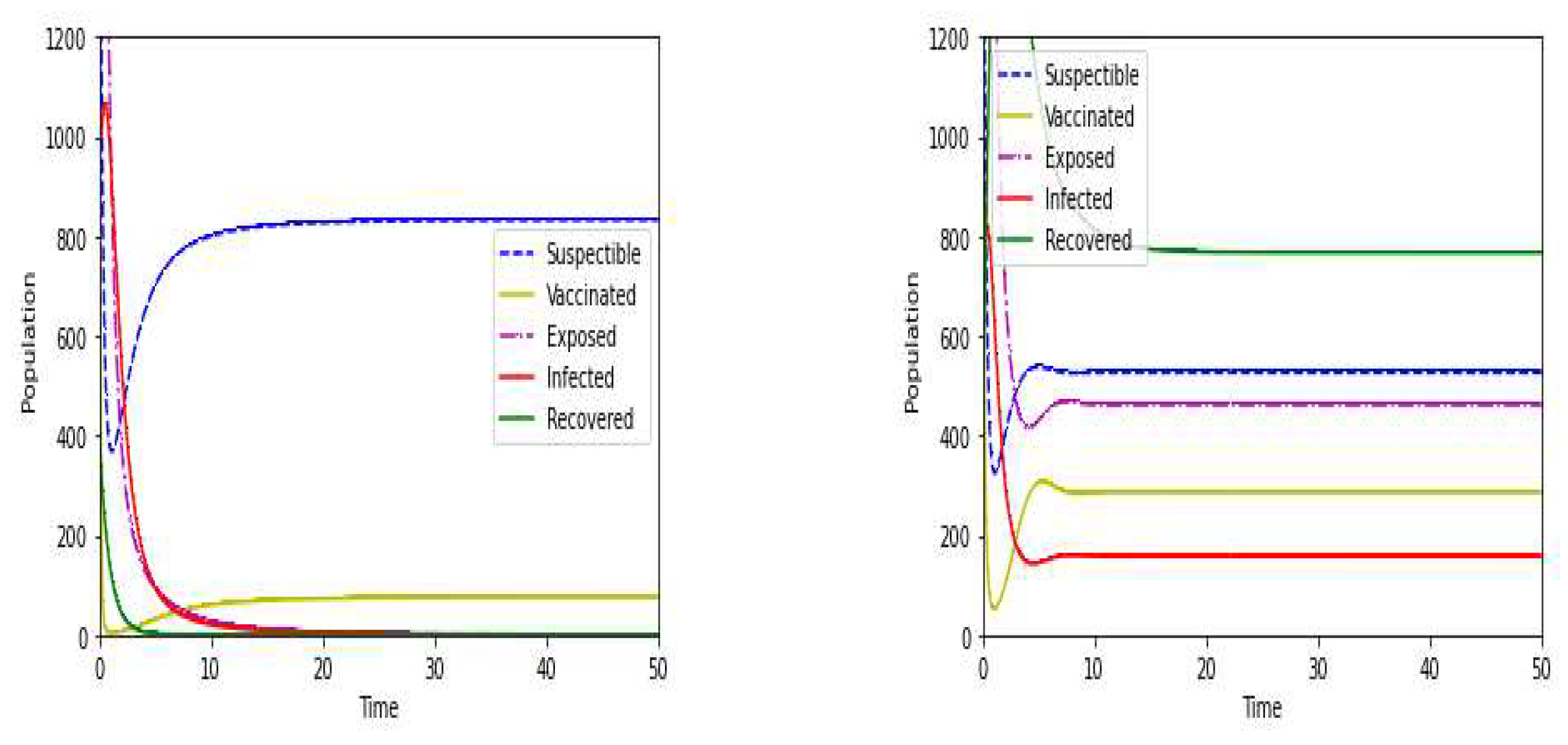
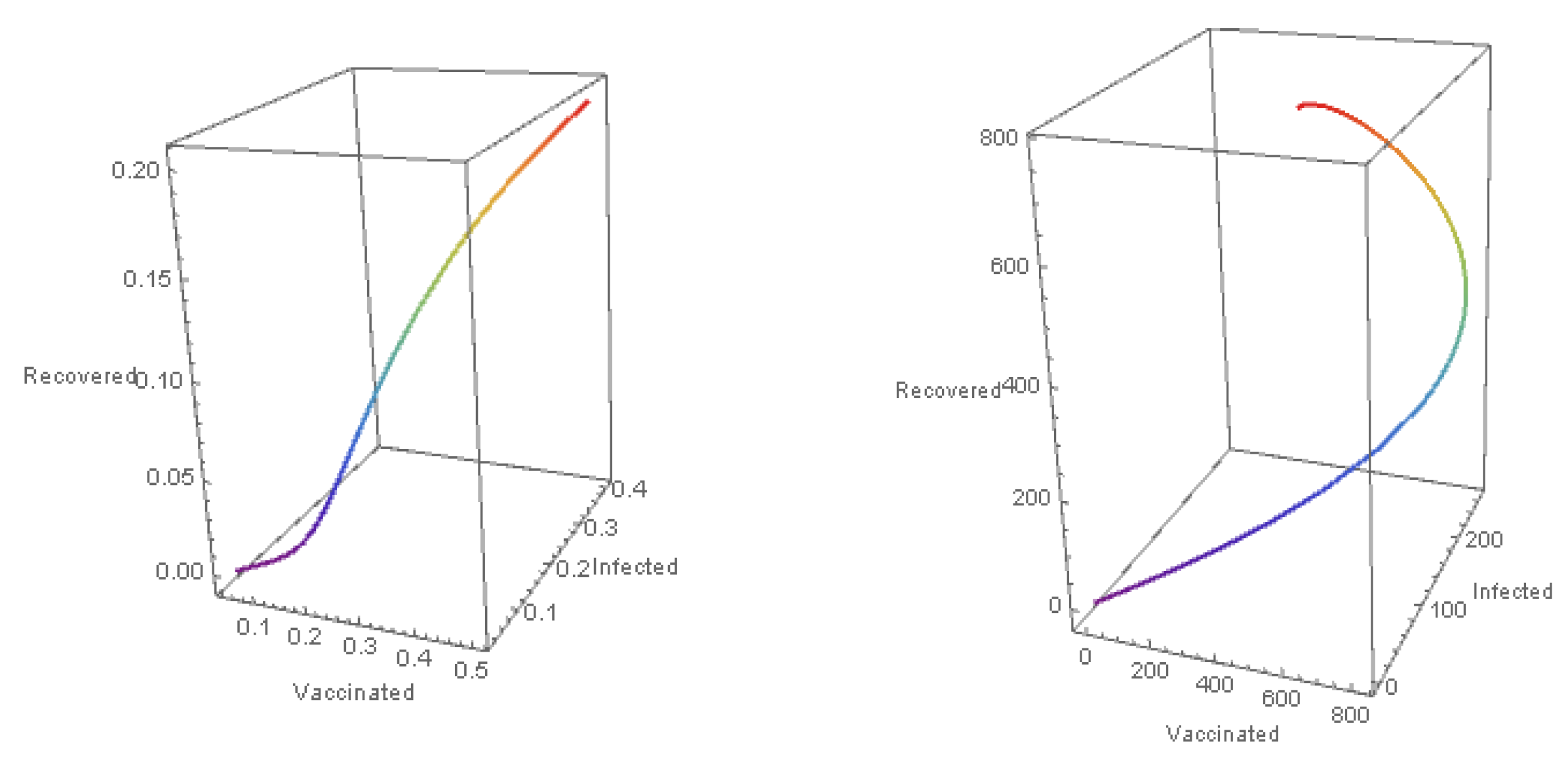
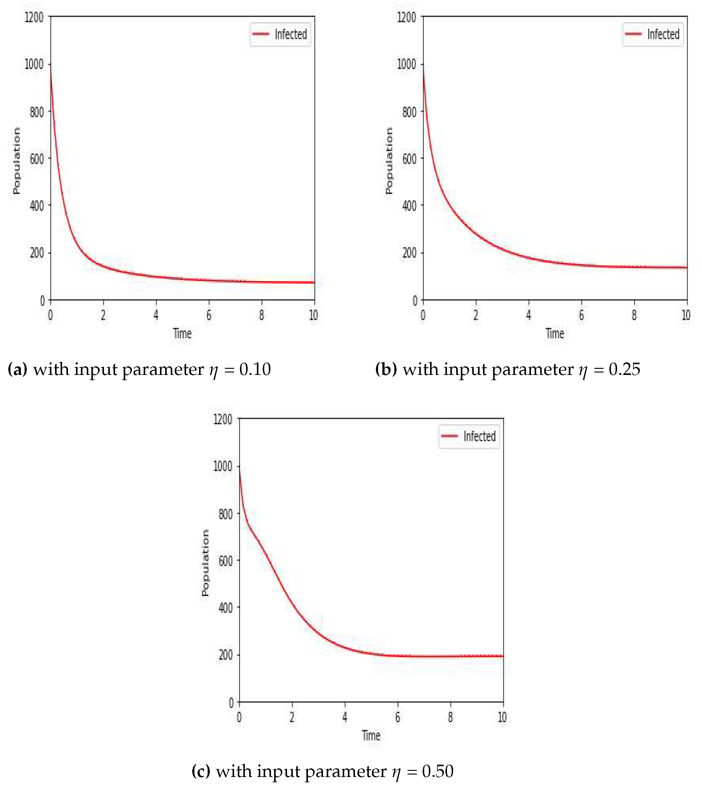
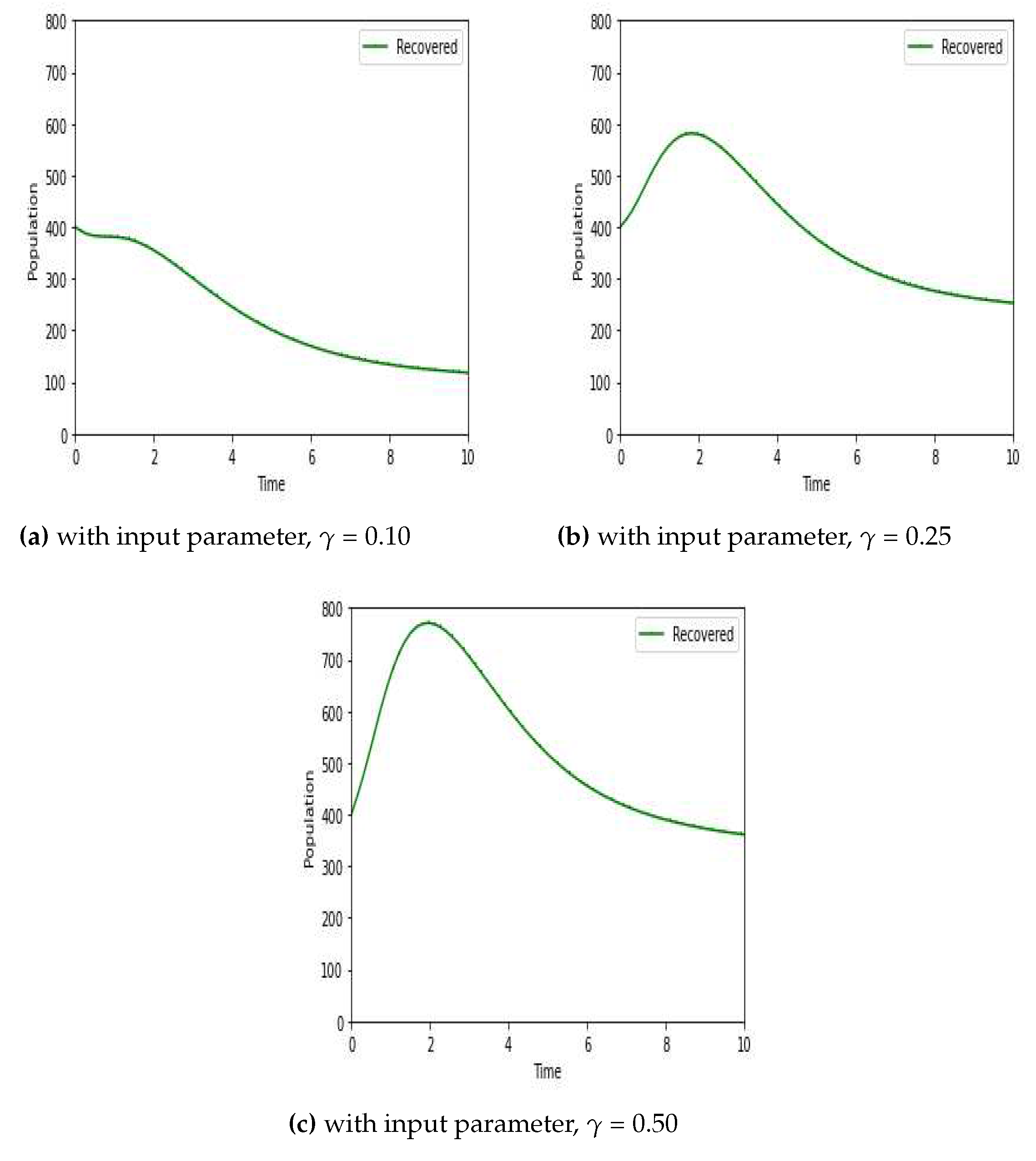
The numerical scheme described above is employed to obtain the numerical results. Furthermore, assumptions are introduced for the initial states of variables and input parameters to streamline the calculations. Figure 1, Figure 2, Figure 3 and Figure 4 show the results of the most effective cases. Figure 1a shows the local stability of

S V E I R

individuals for the corresponding disease free equilibrium. Let us consider,

A = 1000

δ_{1} = 0.0009

δ_{2} = 0.0008

δ_{3} = 0.009

δ_{4} = 0.0008

μ = 0.9

μ_{1} = 0.042

z = 0.099

α_{0} = 0.05

α_{1} = 0.005

γ = 0.0052

and

η = 0.7

. For this set of parameter values we obtain BRN

R_{0} < 1

. So from this we clearly sum up that our

E_{0}

is locally stable. For different set of parameter we get

R_{0} > 1

, which was illustrated in the Figure 1b. So from this we sum up that our

E_{1}

is locally stable. Figure 2a,b shows the phase diagram for vaccinated, infected and recovered population of both DFE and EE. Next, we checked the influence of progression rate for infected individuals, which was depicted in the Figure 3. For this simulation we consider progression rate as 0.10, 0.25, 0.50 respectively. Then we also checked the influence of recovery rate due to treatment for recovered individuals, which was shown in Figure 4. For this simulation we consider recovery rate as 0.10, 0.25, 0.50 respectively. Our analysis predicts that how the input factors influence the output of the system of HFMD transmission.

8. Conclusion

In this study, we focus on investigating the applicability of the CFO mathematical model in understanding the spread dynamics of Hand Foot Mouth Disease (HFMD). The focus of our investigation is to determine whether the system is non negative and bounded, which allowed us to analyse the stability of the model. Through nonlinear analysis, we demonstrated the existence and uniqueness of the model, which enhances its reliability in predicting disease spread. Furthermore, we calculated the numerical solution of the suggested system using the fractional Euler’s approach. This approach is widely used to solve fractional differential equations, and it provides accurate results that are vital in disease modelling. By utilizing this method, we were able to obtain precise solutions for the model, which allowed us to make better predictions about HFMD transmission. Overall, our study demonstrates that the Caputo fractional order mathematical model is a reliable tool for understanding the spread of HFMD. The establishment of positive invariance and boundedness of the system, coupled with the use of nonlinear analysis and numerical solution, enhances the accuracy of the model, which can be used to inform policies aimed at controlling and preventing the spread of HFMD.

Author Contributions

Conceptualization, A.M. and G.C.; methodology, A.M., G.C. and M.Z.M.; software, A.H.M.; validation, A.M. and A.H.M.; formal analysis, A.M. and G.C.; investigation, A.M.; resources, A.M. and A.H.M; data curation, A.H.M.; writing—original draft preparation, A.M., G.C. and M.Z.M.; writing—review and editing, A.M. and A.H.M.; visualization, A.M. and M.Z.M.; supervision, G.C. and A.H.M.; project administration, M.Z.M.; funding acquisition, M.Z.M. All authors have read and agreed to the published version of the manuscript.

Acknowledgments

The authors extend their appreciation to the Deputyship for Research and Innovation, Ministry of Education in Saudi Arabia for funding this research work through the project number ISP-2024.

Conflicts of Interest

The authors declare no conflict of interest.

References

Santhosh kumar, G.; Gunasundari, C. Turing instability of a Diffusive Predator-Prey Model along with an Allee Effect on a Predator. Commun. Math. Biol. Neurosci. 2022, 40, 1–15. [Google Scholar] [CrossRef]
Sharmila, N.B.; Gunasundari, C. Travelling Wave Solutions for a Diffusive Prey-Predator Model with One Predator and Two Preys. Int. J. Appl. Math. 2022, 35. [Google Scholar] [CrossRef]
Aakash, M.; Gunasundari, C.; Qasem, M. Al-Mdallal. Mathematical modeling and simulation of SEIR model for COVID-19 outbreak: A case study of Trivandrum. Front. Appl. Math. Stat. 2023, 9. [Google Scholar] [CrossRef]
Aakash, M.; Gunasundari, C. Effect of Partially and Fully Vaccinated Individuals in some Regions of India: A Mathematical Study on COVID-19 Outbreak. Commun. Math. Biol. Neurosci. 2023, 25. [Google Scholar] [CrossRef]
Abdulaziz, A.; Famara, S.; Mouna, L.; Magloire, P.N.; Francis, B.B.; Ilka, E.; Enagnon, K.A.; Didier, H. Enteroviruses and Type 1 Diabetes Mellitus: An Overlooked Relationship in Some Regions. Microorganisms. 2020, 8. [Google Scholar] [CrossRef]
Syed, Z.S.; Basit, J.; Muhammad, U.M.; Muhammad, W.; Shahkaar, A.; Sobia, A.H.; Amjad, A.; Shazia, R.; Muhammad, I.; Asaad, K.; Ashraf, N. A; Ajmal, K. An Immunoinformatics Approach to Design a Potent Multi-Epitope Vaccine against Asia-1 Genotype of Crimean-Congo Haemorrhagic Fever Virus Using the Structural Glycoproteins as a Target. Vaccines. 2023, 61. [Google Scholar] [CrossRef]
Sivakumar, S.; Moni, S.I.A.; Aamena, J.; Mohammed, E.E.; Duaa, A.; Gassem, G.; Bassem, O.; Abdulla, M.F.; Ahmed, A.J.; Mahdi, M.A.; Alnajai, A.M.H.M.A. Advancements in Vaccine Adjuvants: The Journey from Alum to Nano Formulations. Vaccines. 2023, 11. [Google Scholar] [CrossRef]
Nageswara, R.S.; Ahmed, H.M.; Manoj, S.; Abdullah, A.H.A. ; Existence and Uniqueness for a system of Caputo-Hadamard Fractional Differential Equations with Multipoint Boundary Conditions. Journal of Function Spaces. 2020. [Google Scholar] [CrossRef]
Li, X. P; DarAssi, M.H.; Khan, M.A.; Chukwu, C.W.; Mohammad, Y.A.; mesfer, A.S.; Muhammad, B.R. Assessing the potential impact of COVID-19 Omicron variant: Insight through a fractional piecewise model. Results Phys. 2022, 38. [Google Scholar] [CrossRef]
Kumar, P.R.; Haloi, R.; Bahuguna, D.; Dwijendra, N.P. Existence of solutions to a new class of abstract non-instantaneous impulsive fractional integro-differential equations. Nonlinear Dyn. Syst. Theory. 2016, 16, 73–85. [Google Scholar]
Atangana, A.; Baleanu, D. New fractional derivatives with nonlocal and non-singular kernel: Theory and application to heat transfer model. Therm Sci. 2016, 20, 763–769. [Google Scholar] [CrossRef]
Fatmawati, E.M.; Shaiful, M.I.; Utoyo. A fractional-order model for HIV dynamics in a two-sex population. Int. J. Math. Math. Sci. 2018, 2018, 763–769. [Google Scholar]
Bonyah, E.; Zarin, R.; Fatmawati, E.M. Mathematical modeling of cancer and hepatitis co-dynamics with non-local and non-singular kernel. Commun. Math. Biol. Neurosci. 2020. [Google Scholar] [CrossRef]
Tarasova, V.V.; Tarasov, V.E. Comments on the article long and short memory in economics: fractional-order difference and differentiation. Probl. Mod. Sci. Educ. 2017, 31. [Google Scholar]
Wang, W.; Khan, M.A.; Fatmawati. ; Kumam.; Thounthong, P. A Comparison study of bank data in fractional calculus. Chaos Solitons Fractals. 2019, 126. [Google Scholar] [CrossRef]
Sharmila, N.B.; Gunasundari, C. Stability Analysis of a Fractional Order Prey-Predator Model with Disease in Preys. Mathematica Applicanda. 2022, 50, 287–302. [Google Scholar] [CrossRef]
Nortey, S.N.; Juga, M.; Bonyah, E. Fractional order modelling of Anthrax-Listeriosis coinfection with nonsingular Mittag Leffler law. Scientific African. 2022, 16, 287–302. [Google Scholar] [CrossRef]
Belgaid, Y.; Helal, M.; Lakmeche, A.; Venturino, E. Mathematical Study of a Coronavirus Model with the Caputo Fractional-Order Derivative. Fractal Fract. 2021, 5. [Google Scholar] [CrossRef]
Choi, S.K.; Kang, B.; Koo, N. Stability for Caputo fractional differential systems. Abstr. Appl. Anal. 2014, 2014. [Google Scholar] [CrossRef]
Askar, S.S.; Ghosh, D.; Santra, P.K.; Elsadany, A.A. Mahapatra, G.S, (2021), A fractional order SITR mathematical model for forecasting of transmission of COVID-19 of India with lockdown effect. Results in Physics. 2021, 24. [Google Scholar] [CrossRef]
Aakash, M.; Gunasundari, C.; Rashid, J. Modelling and Analysis of Vaccination Effects on Hand, Foot, and Mouth Disease Transmission Dynamics. Mathematical Modelling of Engineering Problems. 2023, (accepted; in press). [CrossRef]

Figure 1. (a) Variation of S, V, E, I, R for

E_{0}

when BRN is less than one and (b) Variation of S, V, E, I, R for

E_{1}

when BRN is greater than one.

Figure 1. (a) Variation of S, V, E, I, R for

E_{0}

when BRN is less than one and (b) Variation of S, V, E, I, R for

E_{1}

when BRN is greater than one.

Figure 2. Three dimensional Phase diagram of V, I, R for corresponding (a)

E_{0}

and (b)

E_{1}

Figure 2. Three dimensional Phase diagram of V, I, R for corresponding (a)

E_{0}

and (b)

E_{1}

Figure 3. Dynamical behaviour of infected individuals,

Figure 4. Dynamical behaviour of recovered individuals,

Table 1. Overview of the Parameters.

Parameter	Description
A	Rate of recruitment.
$δ_{1}$	Rate of transmission from I to S.
$δ_{2}$	Rate of transmission from E to S.
$δ_{3}$	Rate of transmission from infected to vaccinated.
$δ_{4}$	Rate of transmission from exposed to vaccinated.
$μ$	Natural death rate
$α_{1}$	Transmission from recovered to vaccinated.
$η$	Rate of progression from exposed to infected.
$γ$	Rate of recovery.
$μ_{1}$	Death due to HFMD disease.
$α_{0}$	Rate from recovered to susceptible.
z	Rate of vaccination.

Disclaimer/Publisher’s Note: The statements, opinions and data contained in all publications are solely those of the individual author(s) and contributor(s) and not of MDPI and/or the editor(s). MDPI and/or the editor(s) disclaim responsibility for any injury to people or property resulting from any ideas, methods, instructions or products referred to in the content.

© 2023 by the authors. Licensee MDPI, Basel, Switzerland. This article is an open access article distributed under the terms and conditions of the Creative Commons Attribution (CC BY) license (http://creativecommons.org/licenses/by/4.0/).

Copyright: This open access article is published under a Creative Commons CC BY 4.0 license, which permit the free download, distribution, and reuse, provided that the author and preprint are cited in any reuse.

MDPI Initiatives

Important Links

Choose an area of interest and we will send you notifications of new preprints at your preferred frequency.

Disclaimer

Fractional Order Mathematical Modelling of HFMD Transmission via Caputo Derivative

Abstract

1. Introduction

2. Model Formulation

3. Preliminaries

4. Positivity and Boundedness

5. Existence and Uniqueness

6. Model Analysis

6.1. Equilibrium Points

6.2. Basic Reproduction Number (BRN)

6.3. Local stability

7. Numerical Simulation

8. Conclusion

Author Contributions

Acknowledgments

Conflicts of Interest

References

MDPI Initiatives

Important Links

Subscribe