Submitted:
15 December 2023
Posted:
15 December 2023
You are already at the latest version
Abstract
Keywords:
1. Introduction
2. Methodology
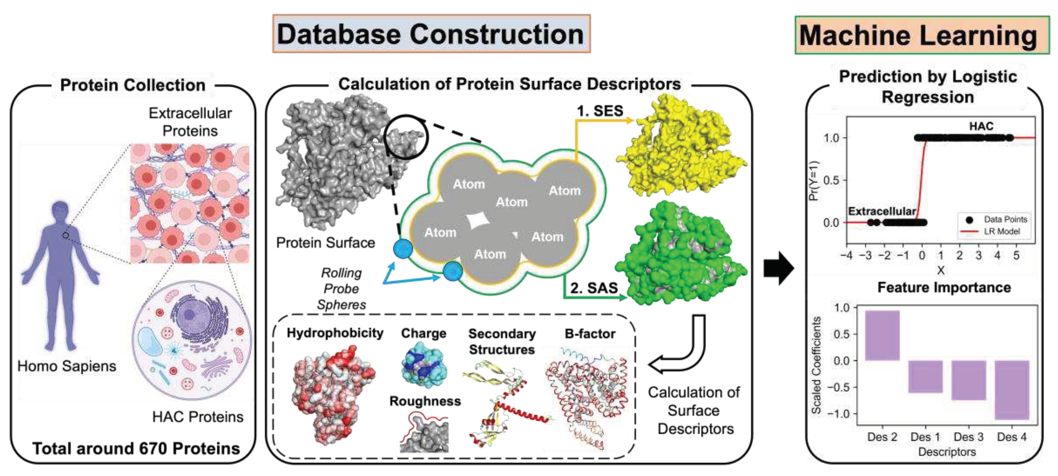
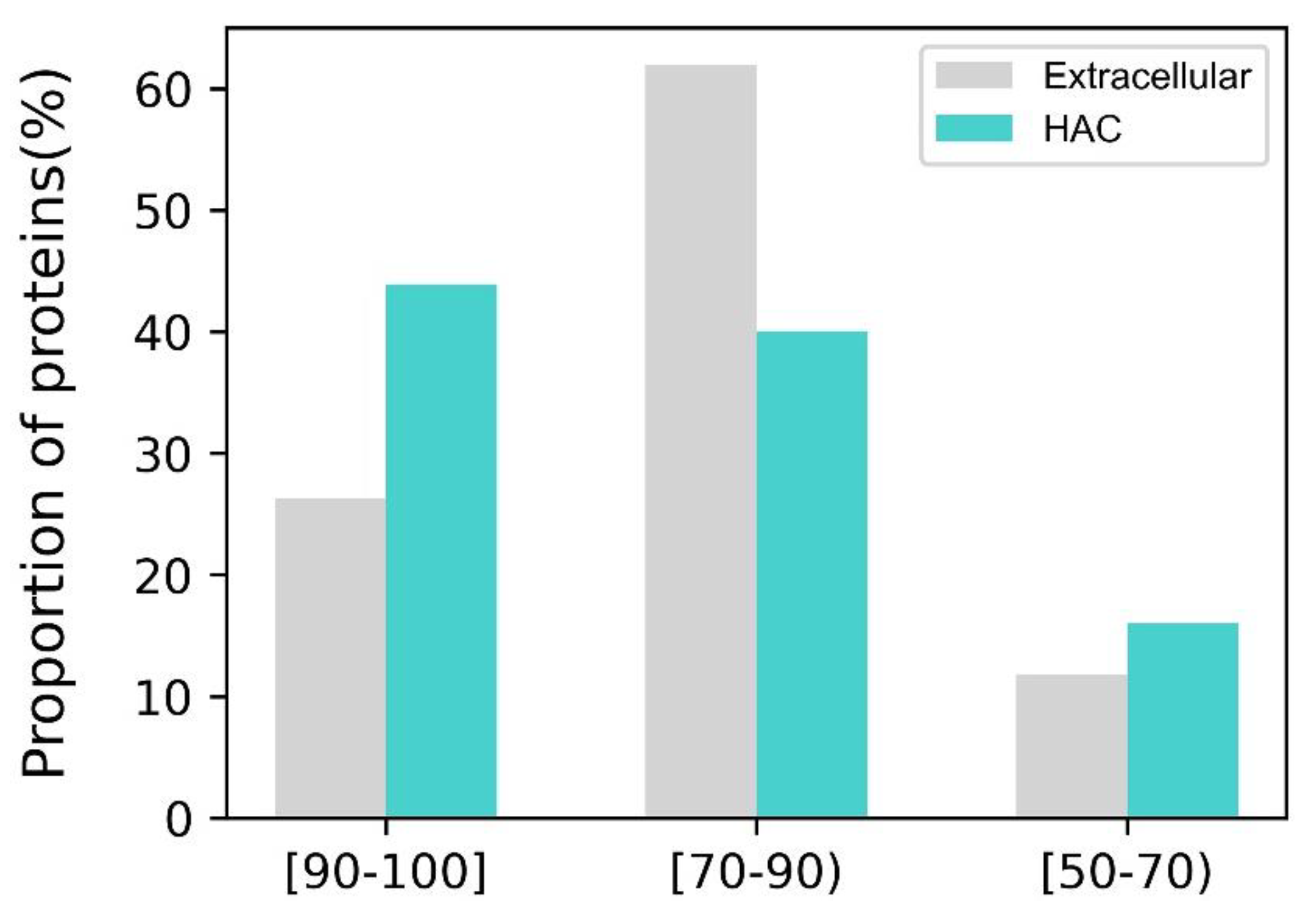
2.1. Protein Sample Collection
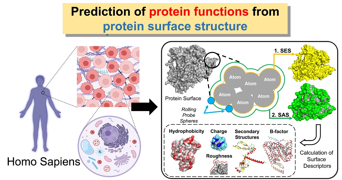
2.2. Calculation of Surface Descriptors
2.3. Application of Machine Learning
4. Results and Discussion
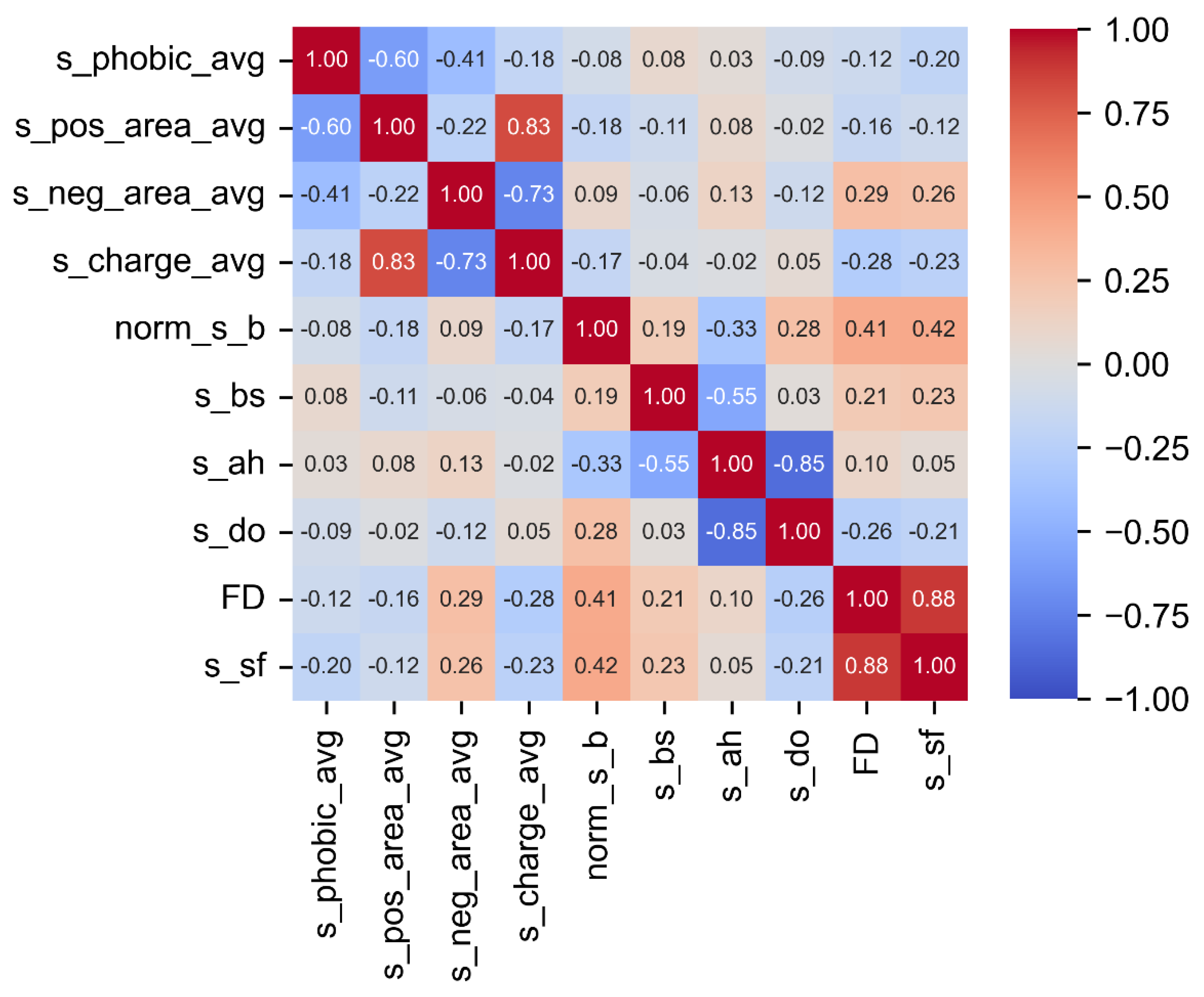
4.1. Pearson Correlation (PC) Analysis
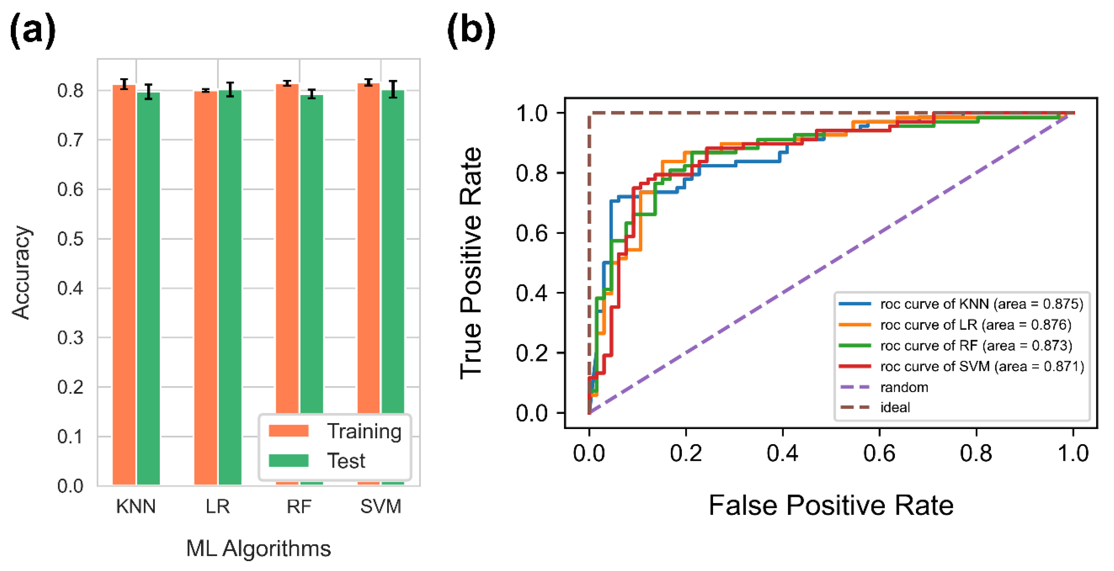
4.2. Comparison of Supervised Machine Learning Algorithms for Binary Classification Problem
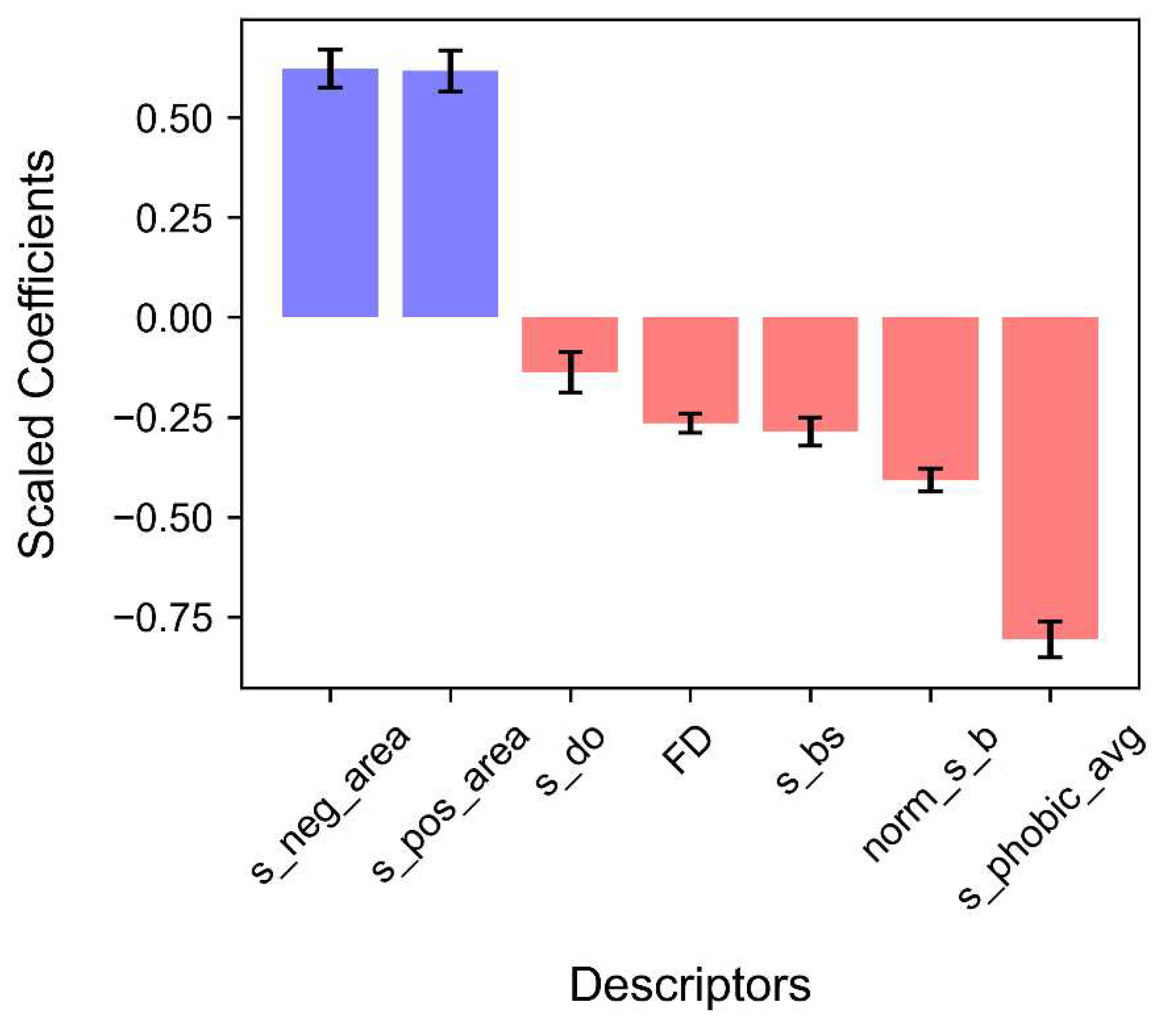
4.3. Results of Logistic Regression Analysis
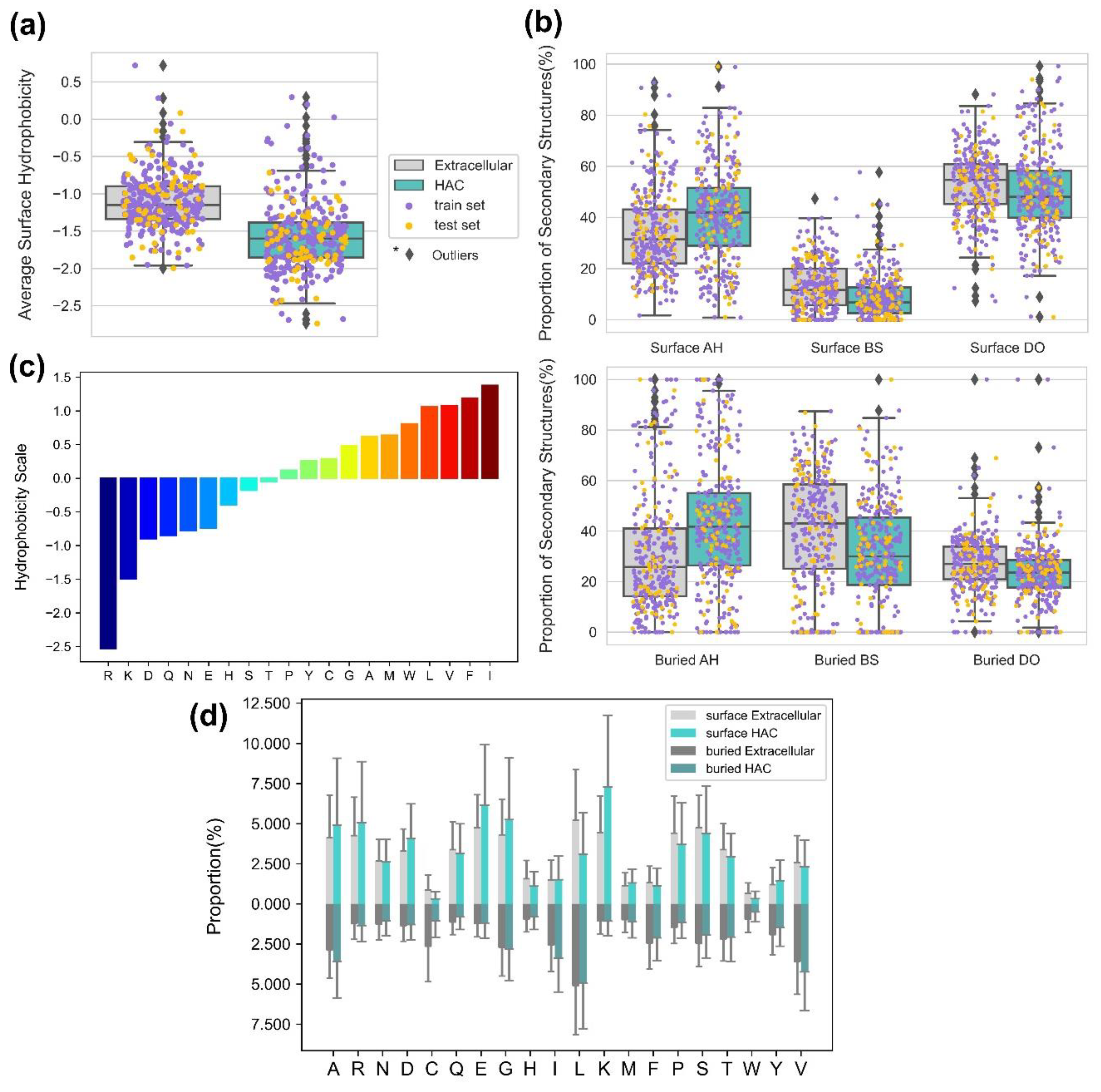
4.4. Proper Folding of HAC Proteins Can Be Achieved with Low Surface Hydrophobicity and Secondary Structure Compositions
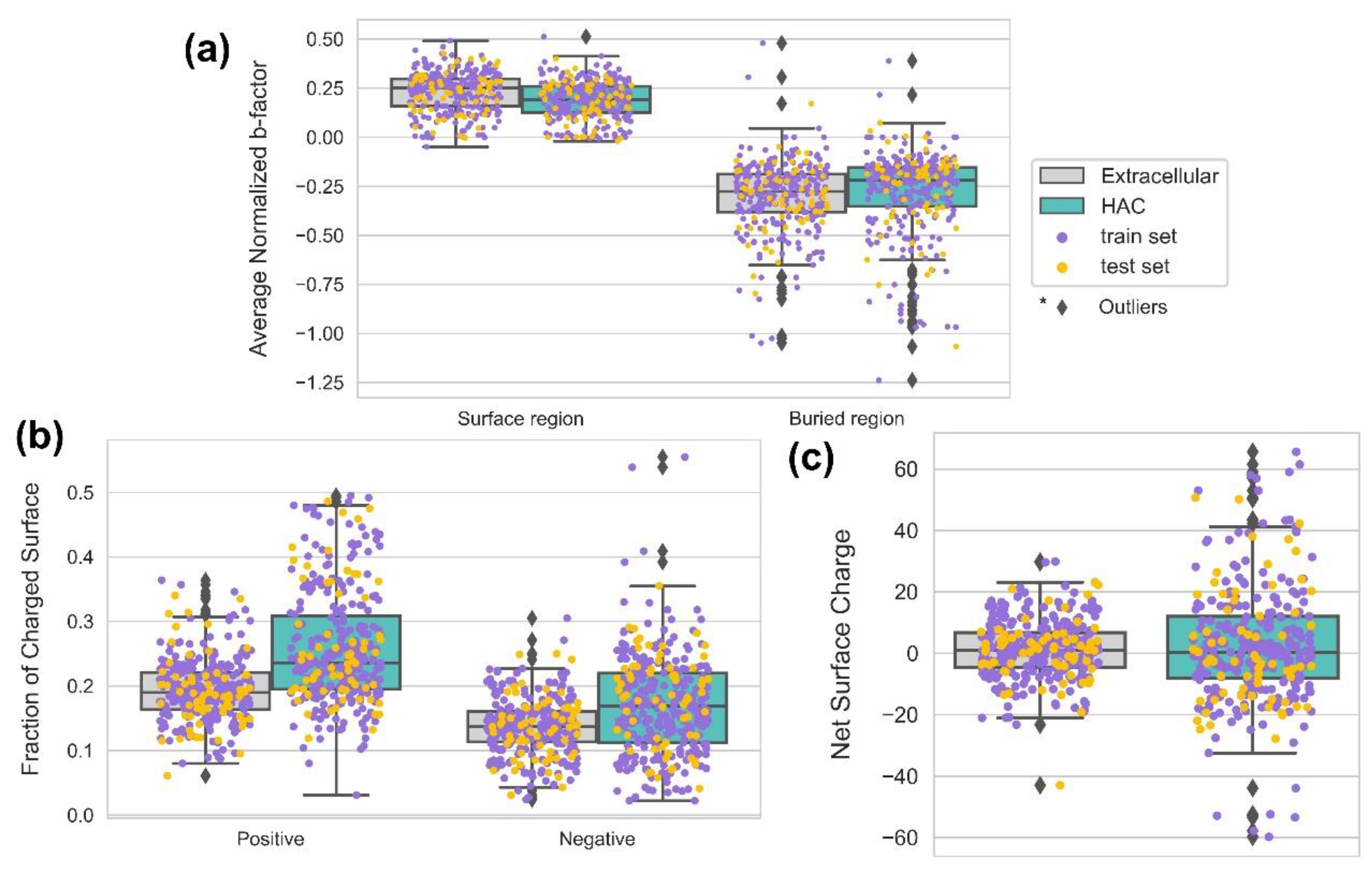
4.5. The HAC Proteins Are Emphasized with Surface Rigidity and an Extreme Range of net Surface Charge
4.6. The Smoother Surface of HAC Proteins May Modulate Molecular Adsorption
5. Summary and Conclusions
Acknowledgments
References
- Ellis, R.J. Macromolecular crowding: obvious but underappreciated. Trends Biochem Sci 2001, 26, 597–604. [Google Scholar] [CrossRef] [PubMed]
- Barbieri, L.; Luchinat, E.; Banci, L. Protein interaction patterns in different cellular environments are revealed by in-cell NMR. Sci Rep 2015, 5, 14456. [Google Scholar] [CrossRef] [PubMed]
- Despa, F.; Orgill, D.P.; Lee, R.C. Molecular crowding effects on protein stability. Ann N Y Acad Sci 2005, 1066, 54–66. [Google Scholar] [CrossRef] [PubMed]
- Frutiger, A.; Tanno, A.; Hwu, S.; Tiefenauer, R.F.; Vörös, J.; Nakatsuka, N. Nonspecific Binding-Fundamental Concepts and Consequences for Biosensing Applications. Chem Rev 2021, 121, 8095–8160. [Google Scholar] [CrossRef] [PubMed]
- Siddiqui, G.A.; Naeem, A. Connecting the Dots: Macromolecular Crowding and Protein Aggregation. J Fluoresc 2023, 33, 1–11. [Google Scholar] [CrossRef]
- Levy, E.D.; Michnick, S.W.; Landry, C.R. Protein abundance is key to distinguish promiscuous from functional phosphorylation based on evolutionary information. Philos Trans R Soc Lond B Biol Sci 2012, 367, 2594–2606. [Google Scholar] [CrossRef] [PubMed]
- van den Berg, B.; Ellis, R.J.; Dobson, C.M. Effects of macromolecular crowding on protein folding and aggregation. EMBO J 1999, 18, 6927–6933. [Google Scholar] [CrossRef] [PubMed]
- Loos, M.S.; Ramakrishnan, R.; Vranken, W.; Tsirigotaki, A.; Tsare, E.P.; Zorzini, V.; Geyter, J.; Yuan, B.; Tsamardinos, I.; Klappa, M.; et al. Structural Basis of the Subcellular Topology Landscape of. Front Microbiol 2019, 10, 1670. [Google Scholar] [CrossRef] [PubMed]
- White, A.D.; Nowinski, A.K.; Huang, W.; Keefe, A.J.; Sun, F.; Jiang, S. Decoding nonspecific interactions from nature. Chemical Science 2012, 3, 3488–3494. [Google Scholar] [CrossRef]
- Levy, E.D.; De, S.; Teichmann, S.A. Cellular crowding imposes global constraints on the chemistry and evolution of proteomes. Proc Natl Acad Sci U S A 2012, 109, 20461–20466. [Google Scholar] [CrossRef] [PubMed]
- Mer, A.S.; Andrade-Navarro, M.A. A novel approach for protein subcellular location prediction using amino acid exposure. BMC Bioinformatics 2013, 14, 342. [Google Scholar] [CrossRef] [PubMed]
- Casadio, R.; Martelli, P.L.; Savojardo, C. Machine learning solutions for predicting protein–protein interactions. WIREs Computational Molecular Science 2022, 12, e1618. [Google Scholar] [CrossRef]
- Crampon, K.; Giorkallos, A.; Deldossi, M.; Baud, S.; Steffenel, L.A. Machine-learning methods for ligand–protein molecular docking. Drug Discovery Today 2022, 27, 151–164. [Google Scholar] [CrossRef] [PubMed]
- Zhang, T.; Gu, J.; Wang, Z.; Wu, C.; Liang, Y.; Shi, X. Protein Subcellular Localization Prediction Model Based on Graph Convolutional Network. Interdiscip Sci 2022, 14, 937–946. [Google Scholar] [CrossRef] [PubMed]
- Jumper, J.; Evans, R.; Pritzel, A.; Green, T.; Figurnov, M.; Ronneberger, O.; Tunyasuvunakool, K.; Bates, R.; Žídek, A.; Potapenko, A.; et al. Highly accurate protein structure prediction with AlphaFold. Nature 2021, 596, 583–589. [Google Scholar] [CrossRef] [PubMed]
- Fam, S.Y.; Chee, C.F.; Yong, C.Y.; Ho, K.L.; Mariatulqabtiah, A.R.; Tan, W.S. Stealth Coating of Nanoparticles in Drug-Delivery Systems. Nanomaterials (Basel) 2020, 10. [Google Scholar] [CrossRef] [PubMed]
- Wang, M.; Weiss, M.; Simonovic, M.; Haertinger, G.; Schrimpf, S.P.; Hengartner, M.O.; von Mering, C. PaxDb, a database of protein abundance averages across all three domains of life. Mol Cell Proteomics 2012, 11, 492–500. [Google Scholar] [CrossRef] [PubMed]
- Ashburner, M.; Ball, C.A.; Blake, J.A.; Botstein, D.; Butler, H.; Cherry, J.M.; Davis, A.P.; Dolinski, K.; Dwight, S.S.; Eppig, J.T.; et al. Gene ontology: tool for the unification of biology. The Gene Ontology Consortium. Nat Genet 2000, 25, 25–29. [Google Scholar] [CrossRef] [PubMed]
- Varadi, M.; Anyango, S.; Deshpande, M.; Nair, S.; Natassia, C.; Yordanova, G.; Yuan, D.; Stroe, O.; Wood, G.; Laydon, A.; et al. AlphaFold Protein Structure Database: massively expanding the structural coverage of protein-sequence space with high-accuracy models. Nucleic Acids Res 2022, 50, D439–D444. [Google Scholar] [CrossRef] [PubMed]
- Mariani, V.; Biasini, M.; Barbato, A.; Schwede, T. lDDT: a local superposition-free score for comparing protein structures and models using distance difference tests. Bioinformatics 2013, 29, 2722–2728. [Google Scholar] [CrossRef]
- Tunyasuvunakool, K.; Adler, J.; Wu, Z.; Green, T.; Zielinski, M.; Žídek, A.; Bridgland, A.; Cowie, A.; Meyer, C.; Laydon, A.; et al. Highly accurate protein structure prediction for the human proteome. Nature 2021, 596, 590–596. [Google Scholar] [CrossRef] [PubMed]
- Ruff, K.M.; Pappu, R.V. AlphaFold and Implications for Intrinsically Disordered Proteins. J Mol Biol 2021, 433, 167208. [Google Scholar] [CrossRef] [PubMed]
- Guo, H.B.; Perminov, A.; Bekele, S.; Kedziora, G.; Farajollahi, S.; Varaljay, V.; Hinkle, K.; Molinero, V.; Meister, K.; Hung, C.; et al. AlphaFold2 models indicate that protein sequence determines both structure and dynamics. Sci Rep 2022, 12, 10696. [Google Scholar] [CrossRef] [PubMed]
- Morris, O.M.; Torpey, J.H.; Isaacson, R.L. Intrinsically disordered proteins: modes of binding with emphasis on disordered domains. Open Biology 2021, 11, 210222. [Google Scholar] [CrossRef]
- Maglic, J.B.; Lavendomme, R. MoloVol: an easy-to-use program for analyzing cavities, volumes and surface areas of chemical structures. J Appl Crystallogr 2022, 55, 1033–1044. [Google Scholar] [CrossRef] [PubMed]
- Lewis, M.; Rees, D.C. Fractal surfaces of proteins. Science 1985, 230, 1163–1165. [Google Scholar] [CrossRef]
- Eisenberg, D.; Schwarz, E.; Komaromy, M.; Wall, R. Analysis of membrane and surface protein sequences with the hydrophobic moment plot. J Mol Biol 1984, 179, 125–142. [Google Scholar] [CrossRef]
- Debye, P. Interferenz von Röntgenstrahlen und Wärmebewegung. Annalen der Physik 1913, 348, 49–92. [Google Scholar] [CrossRef]
- Trueblood, K.N.; Burgi, H.-B.; Burzlaff, H.; Dunitz, J.D.; Gramaccioli, C.M.; Schulz, H.H.; Shmueli, U.; Abrahams, S.C. Atomic Dispacement Parameter Nomenclature. Report of a Subcommittee on Atomic Displacement Parameter Nomenclature. Acta Crystallographica Section A 1996, 52, 770–781. [Google Scholar] [CrossRef]
- Parthasarathy, S.; Murthy, M.R. Protein thermal stability: insights from atomic displacement parameters (B values). Protein Eng 2000, 13, 9–13. [Google Scholar] [CrossRef] [PubMed]
- Vihinen, M. Relationship of protein flexibility to thermostability. Protein Eng 1987, 1, 477–480. [Google Scholar] [CrossRef] [PubMed]
- Yuan, Z.; Zhao, J.; Wang, Z.X. Flexibility analysis of enzyme active sites by crystallographic temperature factors. Protein Eng 2003, 16, 109–114. [Google Scholar] [CrossRef] [PubMed]
- Blaisse, M.R.; Fu, B.; Chang, M.C.Y. Structural and Biochemical Studies of Substrate Selectivity in Ascaris suum Thiolases. Biochemistry 2018, 57, 3155–3166. [Google Scholar] [CrossRef] [PubMed]
- Liu, Q.; Li, Z.; Li, J. Use B-factor related features for accurate classification between protein binding interfaces and crystal packing contacts. BMC Bioinformatics 2014, 15 Suppl 16, S3. [Google Scholar] [CrossRef]
- Oeffner, R.D.; Croll, T.I.; Millán, C.; Poon, B.K.; Schlicksup, C.J.; Read, R.J.; Terwilliger, T.C. Putting AlphaFold models to work with phenix.process_predicted_model and ISOLDE. Acta Crystallogr D Struct Biol 2022, 78, 1303–1314. [Google Scholar] [CrossRef]
- Baek, M.; DiMaio, F.; Anishchenko, I.; Dauparas, J.; Ovchinnikov, S.; Lee, G.R.; Wang, J.; Cong, Q.; Kinch, L.N.; Schaeffer, R.D.; et al. , et al. Accurate prediction of protein structures and interactions using a three-track neural network. Science 2021, 373, 871–876. [Google Scholar] [CrossRef]
- Hiranuma, N.; Park, H.; Baek, M.; Anishchenko, I.; Dauparas, J.; Baker, D. Improved protein structure refinement guided by deep learning based accuracy estimation. Nat Commun 2021, 12, 1340. [Google Scholar] [CrossRef]
- Sun, Z.; Liu, Q.; Qu, G.; Feng, Y.; Reetz, M.T. Utility of B-Factors in Protein Science: Interpreting Rigidity, Flexibility, and Internal Motion and Engineering Thermostability. Chem Rev 2019, 119, 1626–1665. [Google Scholar] [CrossRef] [PubMed]
- Schlessinger, A.; Rost, B. Protein flexibility and rigidity predicted from sequence. Proteins 2005, 61, 115–126. [Google Scholar] [CrossRef] [PubMed]
- Voss, N.R.; Gerstein, M. 3V: cavity, channel and cleft volume calculator and extractor. Nucleic Acids Res 2010, 38, W555–562. [Google Scholar] [CrossRef] [PubMed]
- Hosmer Jr, D.W.; Lemeshow, S.; Sturdivant, R.X. Applied logistic regression; John Wiley & Sons: 2013; Vol. 398.
- Gomez, D.; Huber, K.; Klumpp, S. On Protein Folding in Crowded Conditions. J Phys Chem Lett 2019, 10, 7650–7656. [Google Scholar] [CrossRef]
- Tokuriki, N.; Kinjo, M.; Negi, S.; Hoshino, M.; Goto, Y.; Urabe, I.; Yomo, T. Protein folding by the effects of macromolecular crowding. Protein Science 2004, 13, 125–133. [Google Scholar] [CrossRef]
- Minton, A.P. Excluded volume as a determinant of macromolecular structure and reactivity. Biopolymers 1981, 20, 2093–2120. [Google Scholar] [CrossRef]
- Tang, S.; Li, J.; Huang, G.; Yan, L. Predicting Protein Surface Property with its Surface Hydrophobicity. Protein Pept Lett 2021, 28, 938–944. [Google Scholar] [CrossRef]
- Bhattacharjee, N.; Biswas, P. Structural patterns in alpha helices and beta sheets in globular proteins. Protein Pept Lett 2009, 16, 953–960. [Google Scholar] [CrossRef]
- Nishizawa, M.; Walinda, E.; Morimoto, D.; Kohn, B.; Scheler, U.; Shirakawa, M.; Sugase, K. Effects of Weak Nonspecific Interactions with ATP on Proteins. J Am Chem Soc 2021, 143, 11982–11993. [Google Scholar] [CrossRef]
- Vihinen, M. Solubility of proteins. ADMET DMPK 2020, 8, 391–399. [Google Scholar] [CrossRef]
- He, Y.M.; Ma, B.G. Abundance and Temperature Dependency of Protein-Protein Interaction Revealed by Interface Structure Analysis and Stability Evolution. Sci Rep 2016, 6, 26737. [Google Scholar] [CrossRef]
- Leuenberger, P.; Ganscha, S.; Kahraman, A.; Cappelletti, V.; Boersema, P.J.; von Mering, C.; Claassen, M.; Picotti, P. Cell-wide analysis of protein thermal unfolding reveals determinants of thermostability. Science 2017, 355. [Google Scholar] [CrossRef]
- Moore, D.S. Amino acid and peptide net charges: A simple calculational procedure. Biochemical Education 1985, 13, 10–11. [Google Scholar] [CrossRef]
- Kramer, R.M.; Shende, V.R.; Motl, N.; Pace, C.N.; Scholtz, J.M. Toward a Molecular Understanding of Protein Solubility: Increased Negative Surface Charge Correlates with Increased Solubility. Biophysical Journal 2012, 102, 1907–1915. [Google Scholar] [CrossRef]
- Wang, W.; Nema, S.; Teagarden, D. Protein aggregation—Pathways and influencing factors. International Journal of Pharmaceutics 2010, 390, 89–99. [Google Scholar] [CrossRef]
- Rechendorff, K.; Hovgaard, M.B.; Foss, M.; Zhdanov, V.P.; Besenbacher, F. Enhancement of protein adsorption induced by surface roughness. Langmuir 2006, 22, 10885–10888. [Google Scholar] [CrossRef]
- Scopelliti, P.E.; Borgonovo, A.; Indrieri, M.; Giorgetti, L.; Bongiorno, G.; Carbone, R.; Podestà, A.; Milani, P. The effect of surface nanometre-scale morphology on protein adsorption. PLoS One 2010, 5, e11862. [Google Scholar] [CrossRef]
- Ettelt, V.; Ekat, K.; Kämmerer, P.W.; Kreikemeyer, B.; Epple, M.; Veith, M. Streptavidin-coated surfaces suppress bacterial colonization by inhibiting non-specific protein adsorption. J Biomed Mater Res A 2018, 106, 758–768. [Google Scholar] [CrossRef]
- Pettit, F.K.; Bowie, J.U. Protein surface roughness and small molecular binding sites. J Mol Biol 1999, 285, 1377–1382. [Google Scholar] [CrossRef]
- Chang, R.Y.S.; Mondarte, E.A.Q.; Palai, D.; Sekine, T.; Kashiwazaki, A.; Murakami, D.; Tanaka, M.; Hayashi, T. Protein- and Cell-Resistance of Zwitterionic Peptide-Based Self-Assembled Monolayers: Anti-Biofouling Tests and Surface Force Analysis. Front Chem 2021, 9, 748017. [Google Scholar] [CrossRef]
- Hayashi, T.; Sano, K.; Shiba, K.; Iwahori, K.; Yamashita, I.; Hara, M. Critical amino acid residues for the specific binding of the Ti-recognizing recombinant ferritin with oxide surfaces of titanium and silicon. Langmuir 2009, 25, 10901–10906. [Google Scholar] [CrossRef]
- Hayashi, T.; Sano, K.; Shiba, K.; Kumashiro, Y.; Iwahori, K.; Yamashita, I.; Hara, M. Mechanism underlying specificity of proteins targeting inorganic materials. Nano Lett 2006, 6, 515–519. [Google Scholar] [CrossRef]
- Kim, S.O.; Jackman, J.A.; Mochizuki, M.; Yoon, B.K.; Hayashi, T.; Cho, N.J. Correlating single-molecule and ensemble-average measurements of peptide adsorption onto different inorganic materials. Phys Chem Chem Phys 2016, 18, 14454–14459. [Google Scholar] [CrossRef]
- Mochizuki, M.; Oguchi, M.; Kim, S.O.; Jackman, J.A.; Ogawa, T.; Lkhamsuren, G.; Cho, N.J.; Hayashi, T. Quantitative Evaluation of Peptide-Material Interactions by a Force Mapping Method: Guidelines for Surface Modification. Langmuir 2015, 31, 8006–8012. [Google Scholar] [CrossRef] [PubMed]
- Yamashita, K.; Kirimura, H.; Okuda, M.; Nishio, K.; Sano, K.I.; Shiba, K.; Hayashi, T.; Hara, M.; Mishima, Y. Selective nanoscale positioning of ferritin and nanoparticles by means of target-specific peptides. Small 2006, 2, 1148–1152. [Google Scholar] [CrossRef] [PubMed]
- Wen, W.; Yan, X.; Zhu, C.; Du, D.; Lin, Y. Recent Advances in Electrochemical Immunosensors. Anal Chem 2017, 89, 138–156. [Google Scholar] [CrossRef]
- Rampado, R.; Crotti, S.; Caliceti, P.; Pucciarelli, S.; Agostini, M. Recent Advances in Understanding the Protein Corona of Nanoparticles and in the Formulation of "Stealthy" Nanomaterials. Front Bioeng Biotechnol 2020, 8, 166. [Google Scholar] [CrossRef] [PubMed]
| Category | Variables (Descriptors) | Definition | Analyzed Surface |
|---|---|---|---|
| Hydrophobicity | s_phobic_avg | Average Surface Hydrophobicity | Solvent accessible surface |
| Charge | s_pos_area | Fraction of Positively Charged Surface Area | |
| s_neg_area | Fraction of Negatively Charged Surface Area | ||
| s_charge_avg | Fraction of Total Charged Surface Area | ||
| Protein Structure | s_ah | Proportion of Surface Alpha Helix | |
| s_bs | Proportion of Surface Beta Structures | ||
| s_do | Proportion of Surface Disordered Regions | ||
| s_sf | Structure Surface Exposure Degree | ||
| Flexibility | norm_s_b | Average Normalized Surface B-factors | |
| Geometry | FD | Average Protein Surface Roughness | Solvent excluded surface |
| Surface Descriptors | PC Coefficients | |
|---|---|---|
| Hydrophobicity | s_phobic_avg | -0.472 ** |
| Charge | s_pos_area | 0.401 ** |
| s_neg_area | 0.239 ** | |
| s_charge_avg | 0.142 ** | |
| Protein Structures | s_ah | 0.206 ** |
| s_bs | -0.228 ** | |
| s_do | -0.102 * | |
| s_sf | -0.023 | |
| Flexbility | norm_s_b | -0.225 ** |
| Geometry | FD | -0.106 * |
| Logistic Regression Analysis | |||||||
| Descriptors | β | S.E. | z-value | Significant Level | Odds ratio | Exp(β) 95% C.I. | |
| Min | Min | ||||||
| s_phobic_avg | -0.807 | 0.045 | -17.913 | <0.001 | 0.446 | 0.408 | 0.487 |
| s_pos_area_avg | 0.617 | 0.051 | 12.016 | <0.001 | 1.853 | 1.675 | 2.049 |
| s_neg_area_avg | 0.622 | 0.047 | 13.112 | <0.001 | 1.862 | 1.697 | 2.043 |
| norm_s_b | -0.408 | 0.029 | -13.972 | <0.001 | 0.665 | 0.628 | 0.704 |
| s_bs | -0.286 | 0.036 | -7.992 | <0.001 | 0.751 | 0.700 | 0.806 |
| s_do | -0.138 | 0.050 | -2.738 | <0.05 | 0.872 | 0.790 | 0.962 |
| FD | -0.265 | 0.024 | -11.211 | <0.001 | 0.767 | 0.733 | 0.804 |
Disclaimer/Publisher’s Note: The statements, opinions and data contained in all publications are solely those of the individual author(s) and contributor(s) and not of MDPI and/or the editor(s). MDPI and/or the editor(s) disclaim responsibility for any injury to people or property resulting from any ideas, methods, instructions or products referred to in the content. |
© 2023 by the authors. Licensee MDPI, Basel, Switzerland. This article is an open access article distributed under the terms and conditions of the Creative Commons Attribution (CC BY) license (http://creativecommons.org/licenses/by/4.0/).


