From Meso- to Microscopic Stochastic Modeling in Physico-Chemical Processes – the Paradigm of Chemical Reacting Systems

1. Introduction

All the chemical physical processes involve, in an atomistic perspective, a stochastic description of the events, be them reactive, associated with a change of phase (for instance adsorption) [1], or simply with momentum transfer, such as in collisions. Nonetheless, in the overwhelming majority of the cases of practical and theoretical interest, the number of molecules involved is so large to justify a mean field approach, essentially based on the Boltzmannian hypothesis of molecular chaos (the“stosszahlansatz”) [2]. The mean field formulation represents the backbone of the classical theory of chemical reaction kinetics [3,4]. In between the mean-field formulation - expressed in terms of continuous fields evolving in space and time (representing the core of transport theory and of the theory of irreversible processes) [5,6,7] - and molecular simulations, involving force fields and quantum effects [8,9], stochastic models constitute an alternative capable of accounting for thermal and statistical fluctuations [10] and, at the same time, providing an interpretation for the transport equations of continuous theories as evolution equation for the associated probability densities [11,12].

In most of the cases, the stochastic fluctuations controlling the evolution of chemical-physical processes correspond to the superposition of a variety of elementary events at molecular level, subsumed within the evolution equation by simplified stochastic models, the basic property of which lies in their coarse-grainedness (mathematically corresponding to the application of Central Limit Theorem), independently of the specific phenomenology occurring at the molecular level [13]. It is therefore not surprising that these stochastic approaches are essentially based on a Gaussian assumption for the probability densities of the fluctuating perturbations, leading to parabolic models for the transport equations of the classical theory of irreversible processes [6].

However, it is possible to provide alternatives to this approach, defining the stochastic dynamics at a microscopic level, and accounting for the elementary chemical-physical processes involved at this scale. The latter approach, beyond its intrinsic relevance, offers also the way to determine under what conditions the Gaussian approximation in coarse-grained models can be assumed to be valid, and if this is not the case, how specific microscopic interactions may lead to macroscopic transport anomalies.

In this article we address the mathematical formulation of microscopic stochastic modelling using chemical reaction kinetics as a prototypical case study. The rationale in these models is the description of the elementary events (reactive molecular collisions) as distributional derivatives of counting processes [10]. This type of formulation is not only important in the study of chemical reaction kinetics, but it also provides a very flexible conceptual framework for addressing any chemical-physical process in terms of elementary events involving individual molecular entities. Another typical example of this approach is represented by the thermalization dynamics in a molecular mixture controlled by radiative effects and related to the emission and absorption of energy quanta (see Section 6).

The article is organized as follows. Section 2 discusses in detail the multiscale modeling of irreversible processes, the mesoscopic nature of the existing stochastic formulations and the need for a microscopic event-based approach. Section 3 provides a succinct overview on the state of the art in the stochastic modelling of chemical kinetics and on its algorithmic representation. Section 4 addresses the mathematical formulation of stochastic chemical reactions as a paradigm for any event-based microscopic description. Section 5 applies this approach to the clustering of liquid molecules and its influence on the velocity distribution function at thermal equilibrium. Finally, Section 6 analyzes the role of radiative interactions (absorption and emission of photons) in thermalization processes, and the occurrence of deviations from the Gaussian distribution in equilibrium velocity densities.

2. Models of irreversible processes and their multiscale nature

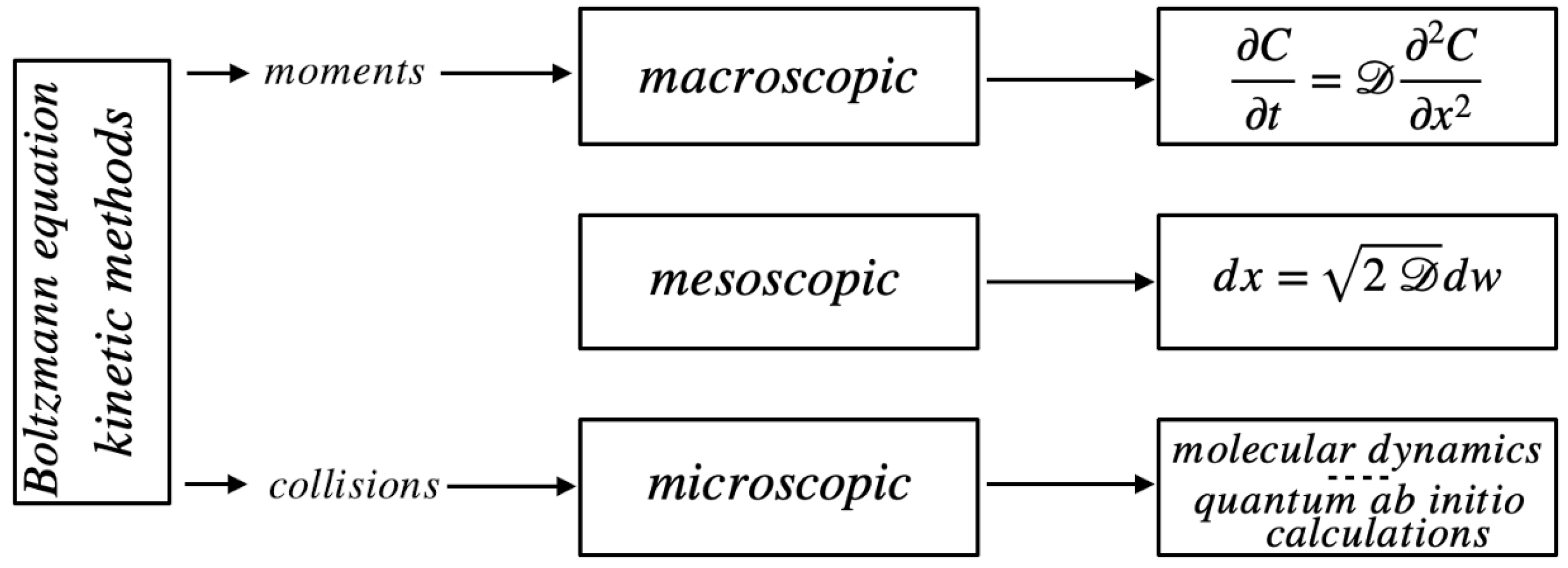
Chemical physical processes can be described at different length scales, depending on the focus/attention on the microscopic interactions. A rough classification of possible representations, customarily adopted, involves three major classes: macroscopic, mesoscopic, and microscopic (Figure 1). The two extrema in this categorization are rather clear. Macroscopic modeling involves the evolution of smooth space-time fields, such, e.g., the solute concentration $c(\mathbf{x},t)$ in a fluid flow, and the resulting dynamics for the continuous fields is expressed in the form of partial differential equations, in most of the cases of parabolic nature (first-order in time, second-order with respect to the spatial variables). At the opposite edge, microscopic models assume the atomistic constitution of matter (molecules) and, considering the interaction between molecules, eventually including quantum effects as regards charge and dipolar moment distributions, describe the evolution of an ensemble of molecular entities via Newtonian equations of motion, complemented with suitable algorithmic/analytic solutions to account for specific thermodynamic conditions (thermostats). The goal of the molecular simulations is essentially to determine the values of transport coefficients and thermodynamic parameters, or the occurrence of phase transitions.

A particular role is played by non-equilibrium kinetic models, such as the Boltzmann equation. Depending on the way they are regarded and utilized, they are able to spam both a microscopic description (as binary collision are explicitly considered, and the collisional integral accounts for the Markovian transitions in the particle velocities controlled by elementary collisional events) [14,15] or the macroscopic transport theory (whenever the lower-order moments are considered to derive the transport equations for the collisional invariants).

In between the two aforementioned cases, there is a sea of intermediate-scale approaches that consistently use stochastic processes to model the effects of fluctuations (be them thermal, deriving from the granularity of matter, or of quantum nature) in a coarse-grained way. These models stem from the pioneering work of Einstein, Langevin, Smoluchowski on Brownian motion [16,17], i.e. the highly erratic kinematics of micrometric particles in a still fluid driven by thermal fluctuations. The equations of motion for the particles/molecules are derived taking into account the presence of hydrodynamics and/or of external potentials, and describing in a coarse-grained way the effects of thermal fluctuations. The statistical description of the stochastic motion of the particles in terms of probability densities corresponds to the macroscopic thermodynamic level involving the spatio-temporal evolution of the concentration fields.

The prototypical example of mean-field stochastic modelling refers to the motion of micrometric particles in a fluid, the hydrodynamic velocity field of which is ${\mathbf{u}}_f\left(\mathbf{x}\right)=(u_{f,1}\left(\mathbf{x}\right),u_{f,2}\left(\mathbf{x}\right),u_{f,3}\left(\mathbf{x}\right))$, $\mathbf{x}\in {\mathbb{R}}^3$. Assuming the size of the particle small compared to the length scale of the velocity variations, and isothermal conditions (constant temperature T), the equation of motion takes the form of a Wiener-driven Langevin equation

$$d\mathbf{x}={\mathbf{u}}_f\left(\mathbf{x}\right)dt+\sqrt{2D}d\mathbf{w}\left(t\right)$$

(1)

where $d\mathbf{w}\left(t\right)=(d{w}_1\left(t\right),d{w}_2\left(t\right),d{w}_3\left(t\right))$ is the increment of a vector-valued Wiener process in the time interval $(t,t+dt)$ (and thus the entries $d{w}_i\left(t\right)$, $i=1,2,3$ are independent of each other), and D the diffusion coefficient. From eq. (2) it follows that the associated probability density $p(\mathbf{x},t)$ satisfies the Fokker-Planck equation

$$\frac{\partial p(\mathbf{x},t)}{\partial t}=-\nabla ·\left[{\mathbf{u}}_f\left(\mathbf{x}\right)p(\mathbf{x},t)\right]+D{\nabla }^{2}p(\mathbf{x},t)$$

(2)

which corresponds to the classical macroscopic advection-diffusion equation of mass transport theory for the solute concentration that, modulo a multiplicative constant, equals the density $p(\mathbf{x},t)$.

Eq. (1) is a mesoscopic description of motion because the transport coefficient controlling the process, i.e. the diffusivity D, is already included into the model without a derivation of it from a microscopic interaction mechanism. Of course one could invoke a more fundamental stochastic description involving the momentum transfer mechanism, as originally formulated by Langevin: if $\mathbf{v}$ is the particle velocity and m its mass then

$$md\mathbf{v}=-\eta \left[\mathbf{v}-{\mathbf{u}}_f\left(\mathbf{x}\right)\right]dt+\sqrt{2k_{B}T\eta }d\mathbf{w}\left(t\right)$$

(3)

where $\eta$ is the friction factor, stemming from the hydrodynamic interactions with the solvent fluid, and $k_B$ the Boltzmann constant. Eq. (2) follows from eq. (3) in the limit of vanishing inertia (overdamped approximation) where $md\mathbf{v}=0$, enforcing

$$d\mathbf{x}=\mathbf{v}dt$$

(4)

and the Stokes-Einstein fluctuation-dissipation relation

$$D=\frac{k_{B}T}{\eta }$$

(5)

connecting the diffusivity D to the hydromechanical properties, expressed by the friction factor $\eta$, and to the thermodynamic conditions of the systems, expressed by the temperature T.

But even eq. (3) is a mesoscopic description of the thermal fluctuations: the use of the Wiener process $\mathbf{w}\left(t\right)$, by its nature, corresponds to a long-term asymptotic characterization, emerging from the superposition of small and independent random pertubations so that the Central Limit Theorem (CLT) can be invoked [18,19].

It is therefore not surprising that the resulting transport equation is of parabolic nature as, by definition of the (one-dimensional) Wiener process $w\left(t\right)$, its increment $y=w\left(t_2\right)-w\left(t_1\right)$ over the time interval $t_2-t_1>0$ is a Gaussian random variable with zero mean and square variance equal to $t_2-t_1$ [13]. Moreover, the increments in two disjoint time intervals are independent of each other. Setting $y=w\left(t\right)-w\left(0\right)=w\left(t\right)$, since $w\left(0\right)=0$ by definition [10], the probability density for y is Gaussian

$$p_y\left(y\right)=p_w{(w,t)|}_{w=y}={\left.\frac{1}{\sqrt{2\pi t}}{e}^{-w^2/2t}\right|}_{w=y}$$

(6)

and $p(w,t)$ so defined is the solution of the diffusion equation

$$\frac{\partial p_w(w,t)}{\partial t}=\frac{1}{2}\frac{{\partial }^2{p}_w(w,t)}{\partial w^2}$$

(7)

Therefore, the choice of Wiener perturbations as the global descriptor of the effects of thermal fluctuations automatically implies that the resulting macroscopic transport equations for the densities are partial differential equations of parabolic nature.

The mesoscopic formulation based on Wiener-Langevin equations of the form eq. (1) represents one of the basic strongholds of contemporary statistical physics. At the same time, this setting shows intrinsic physical limitations in the broader perspective of improving the formulation of macroscopic thermodynamic models. The parabolic nature of the resulting transport equations brings with it inherent inconsistencies such as the paradox of infinite velocity of propagation [7], and this limits its application to generic (and extreme) thermodynamic conditions (such as at very low temperatures), and to generic fluids (more complex that purely Newtonian fluids, such as viscoelastic fluids) [20,21,22]. Moreover, there is no relation between a microscopic theory of mass transport and the properties of the stochastic force, other than the appeal to CLT. As in the absence of the external velocity field (${\mathbf{u}}_f=0$), the statistics of the velocity fluctuations deriving from eq. (3) is Gaussian, there is no indication in this form of mesoscopic stochastic theories of the conditions under which the Gaussian paradigm may fail, and new emergent phenomenologies may arise.

In order to answer these questions, and to provide a framework for describing thermal fluctuations beyond the pure CLT limit, a microscopic stochastic theory of motion is required, where the elementary mechanisms controlling momentum transfer and motion are singled out and accounted for. This may represent a general microscopic approach for handling a huge variety of chemical physical phenomena. The paradigmatic problem of such a microscopic event-based theory is represented by chemical reactions, as addressed in the next two Section 3 and Section 4. In the remainder of the article, we consider several extensions of this approach to the analysis of a model for molecular coalescence in liquids and its implications as regards transport (Section 5) and to the velocity distribution in molecular systems driven by radiative effects (emission and absorptions of photons) (Section 6).

3. Stochastic modelling of chemical kinetics

Consider a typical bimolecular reaction mechanism

$$A+B\to C$$

(8)

where A, B and C indicate the reacting species. The stoichiometry defined by eq. (8) implies that one molecule of A and one molecule of B should collide, and that their kinetic energy is sufficiently high to overcome the activation energy so that the chemical transformation to C may take place.

In a mean-field framework, letting $c_A$, $c_B$ and $c_C$ be the concentrations of the reacting species, and assuming spatial uniformity in a closed reacting vessel, so that these concentrations depend uniquely on time, we have

$$\frac{d{c}_A}{dt}=\frac{d{c}_B}{dt}=-\frac{d{c}_C}{dt}=-k{c}_A{c}_B$$

(9)

where k is the rate constant, accounting for the frequency of occurrence of reactive collisions. It is immediate to recognize that the mean field approach to chemical kinetics corresponds exactly to the “stosszahlansatz” (the hypothesis of molecular chaos) enforced by Boltzmann in deriving his kinetic equation for non-equilibrium processes in diluted gaseous systems.

The latter analogy is indeed highlighting as it indicates the possibility of gathering together momentum-transfer processes, controlling molecular motion, with chemical/quantum events associated with chemical reactions and quantum transitions in a unitary stochastic event-based theory.

The stochastic theory of chemical reactions dates back to the formulation of the chemical master equation developed in order to handle reactive systems in which the granularity (limited and small number of molecules) plays a leading role and controls the statistical fluctuations in small reacting systems.

It is well known that, in all the cases where the number of molecules is small (and this occurs in subcellular biochemical reactions, in nanoscale systems, or in the growth kinetics of microorganisms [23,24,25]), the effects of fluctuations become significant, motivating a stochastic description of chemical kinetic processes, involving the number of molecules present in the system, thus explicitly accounting for their finite number [26,27,28,29]. The statistical theory of chemical kinetics in these conditions is grounded on the Chemical Master Equation (CME) [30,31], expressing the time evolution for the probabilities $p(\mathbf{N},t)$ of all the possible number-configurations $\mathbf{N}\left(t\right)=(N_1\left(t\right),\cdots ,N_s\left(t\right))$, where $N_h\left(t\right)$ is the number of molecules of the h-th reacting species at time t, $h=1,\cdots ,s$. However, apart from a handful of simple cases, for which the CME can be solved analytically [32], numerical methods should be applied to it in order to compute mean values and higher-order moments. But also this choice reveals itself to be unfeasible in most of the situations of practical and theoretical interest, due to the extremely large number of configurations involved, making the multi-index matrix $p(\mathbf{N},t)$ so huge to exceed reasonable computational facilities.

In order to solve this problem, Gillespie proposed an algorithmic solution to the numerical simulation of stochastic reacting systems, based on the Markovian nature of the reactive events [33,34]. The original Gillespie algorithm has been extended and improved over time, providing a variety of slightly different computational alternatives. A common denominator of the first family of the Gillespie algorithms (namely those based on the direct method, the first reaction method or their derivates [35,36,37]) is to associate to every time step the occurrence of just one reaction. This formulation comes directly from the assumption that, if the time step is small enough, the probability that more than one reaction will occur is negligible. While correct, this choice brings to significant computational costs for complex reaction schemes. This problem has been highlighted several times, by the Gillespie group itself, as stiffness in stochastic chemical reacting systems [38]. A brilliant way to overcome this limit has been the famous tau-leaping method, which, unfortunately, requires to check that the propensity functions (i.e., the probabilities of occurrence of the reactive steps) remain almost constant at each iteration and can be applied just if this condition is verified [39,40]. The algorithmic solution associated with the formalism here introduced combines the accuracy of the first stochastic simulation algorithms with the computational advantages of the tau-leaping method.

There is, moreover, a missing link between CME theory and the Gillespie algorithm, consisting in the straight mathematical formulation of the stochastic differential equations associated with a chemical reacting system, the statistical description of which would correspond to the CME. To clarify this issue, consider the conceptually analogous problem of particle diffusion over the real line, the statistical description of which is expressed by the parabolic equation $\partial p(x,t)/\partial t=D{\partial }^{2}p(x,t)/\partial x^2$, for the probability density $p(x,t)$ of finding a particle at position x at time t. Setting $x_n=x\left(n\mathsf{\Delta }t\right)$, an algorithm describing this process can be simply expressed by the discrete evolution equation $x_{n+1}=x_n+\sqrt{2D\mathsf{\Delta }t}{r}_{n+1}$, where $r_h$, $h=1,2,\cdots$ represent independent random variables sampled from a normal distribution (with zero mean, and unit variance) [41]. This represents an efficient algorithmic solution of the problem, whenever the time resolution $\mathsf{\Delta }t$ is small enough. Nevertheless, the mere algorithmic approach cannot be considered physically satisfactory, in a comprehensive formulation of transport theory embedded in a continuous space-time (in which both position x and time t are real valued). In point of fact, only with the mathematical formulation due to K. Ito of stochastic differential equations driven by the increments $dw\left(t\right)$ of a Wiener process (Langevin equations) [42], namely $dx\left(t\right)=\sqrt{2D}dw\left(t\right)$ the theory of diffusive motion has found a proper mathematical physical setting.

A similar situation applies to the case of stochastic models of chemical reaction kinetics, for which up to now, the fundamental representation in terms of stochastic differential equations is missing (see e.g. the review [43]).

4. Stochastic models for chemical reactions

As mentioned above, this article is aimed at overcoming the purely algorithmic description of stochastic chemical reactions, providing the formulation of these processes as stochastic differential equations evolving continuously with time.

The basic idea is that any reactive process corresponds to a system of elementary events (the single reaction) possessing a Markovian transitional structure, and consequently, amenable to a description by means of the increments of counting processes (Poisson processes, in the Markovian case). This topic has been also pointed out in [44] in terms of Poisson measures, although the latter formulation is much less simple and physically intuitive than the approach proposed in the present article.

To begin with, consider the simple case of a first-order chemical reaction $A\underset{k_{-1}}{\stackrel{k_1}{\rightleftharpoons }}B$ (for instance, an isomerization). This model is perfectly analogous to the radiative transition of a molecule possessing two energy states, due to emission and adsorption of an energy quantum (Figure 2). Let $N_A\left(0\right)+N_B\left(0\right)=N_g$ the total number of molecules at time $t=0$. The state of the system is characterized by the state functions ${\sigma }_h\left(t\right)$, $h=1,\cdots ,N_g$ for each molecule, attaining values $\{0,1\}$, and such that ${\sigma }_h\left(t\right)=0$ if the energy state at time t is $E_0$ (or equivalently if the molecule finds itself in the state A), and ${\sigma }_h\left(t\right)=1$ in the opposite case (energy state $E_1$, or isomeric state B).

Let ${\{{\chi }_h^{\left(1\right)}(t,k_1),{\chi }_h^{\left(2\right)}(t,k_{-1})\}}_{h=1}^{N_g}$ be two systems of independent Poisson processes, characterized by the transition rates $k_1$, and $k_{-1}$, respectively. The evolution of ${\sigma }_h\left(t\right)$ can be expressed via the stochastic differential equation

$$\frac{d{\sigma }_h\left(t\right)}{dt}=\left(1-{\sigma }_h\left(t\right)\right)\frac{d{\chi }_h^{\left(1\right)}(t,k_1)}{dt}-{\sigma }_h\left(t\right)\frac{d{\chi }_h^{\left(2\right)}(t,k_{-1})}{dt}$$

(10)

$h=1,\cdots ,N_g$, where $d\chi (t,\lambda )/dt$ is the distributional derivative of the Poisson process $\chi (t,\lambda )$, corresponding to a sequence of unit impulsive functions at the transition instants $t_i^{*}$, $i=1,2,\cdots$, $0<t_i^{*}<t_{i+1}^{*}$, where for $\epsilon >0$, ${lim}_{\epsilon \to 0}{\int }_{t_i^{*}-\epsilon }^{t_i^{*}+\epsilon }d\chi (t,\lambda )=1$. Summing over $h=1,\cdots N_g$, and observing that $N_A\left(t\right)={\sum }_{h=1}^{N_g}\left(1-{\sigma }_h\left(t\right)\right)$, $N_B\left(t\right)={\sum }_{h=1}^{N_g}{\sigma }_h\left(t\right)$, we have

$$\frac{d{N}_B\left(t\right)}{dt}=\sum _{h=1}^{N_A\left(t\right)}\frac{d{\chi }_h^{\left(1\right)}(t,k_1)}{dt}-\sum _{h=1}^{N_B\left(t\right)}\frac{d{\chi }_h^{\left(2\right)}(t,k_{-1})}{dt}$$

(11)

and $d{N}_A\left(t\right)/dt=-d{N}_B\left(t\right)/dt$, representing the evolution equation for $N_A\left(t\right)$ and $N_B\left(t\right)$, attaining integer values. The stochastic evolution of the number of molecules $N_A\left(t\right)$, $N_B\left(t\right)$ is thus expressed as a differential equation with respect to the continuous physical time $t\in {\mathbb{R}}^{+}$, over the increments of a Poisson process. Interpreted in a mean-field way, if $c_{\mathrm{tot}}$ is the overall concentration of the reactants at time $t=0$, then the concentrations $c_{\alpha }\left(t\right)$, $\alpha =A,B$, at time t can be recovered from eq. (11) as

$$c_{\alpha }\left(t\right)=c_{\mathrm{tot}}\frac{N_{\alpha }\left(t\right)}{N_g},\alpha =A,B$$

(12)

representing the calibration relation connecting the stochastic description, in terms of the number of molecules $N_{\alpha }\left(t\right)$, and the concentrations $c_{\alpha }\left(t\right)$, $\alpha =A,B$ entering the mean-field description.

The analytical formulation of a stochastic differential equation for chemical kinetics, expressed in terms of the number of molecules of the chemical species involved, rather than an algorithm defined for discretized times, allows the development of a variety of different numerical strategies, that naturally perform a modified tau-leaping procedure, as the occurrence of several distinct reactive events in any elementary time step $\mathsf{\Delta }t$ is intrinsically accounted for. This can be easily seen by considering the simple reaction defined by the evolution equation (11). In terms of increments, eq. (11) can be written as $d{N}_B\left(t\right)={\sum }_{h=1}^{N_A\left(t\right)}d{\chi }^{\left(1\right)}(t,k_1)-{\sum }_{h=1}^{N_B\left(t\right)}d{\chi }^{\left(2\right)}(t,k_{-1})$. If $\mathsf{\Delta }t$ is the chosen time step, it follows from this formulation, a simple numerical approximation for eq. (11), namely,

$$\mathsf{\Delta }{N}_B\left(t\right)=N_B(t+\mathsf{\Delta }t)-N_B\left(t\right)=\sum _{h=1}^{N_A\left(t\right)}{\xi }_h^{\left(1\right)}\left(k_1\mathsf{\Delta }t\right)-\sum _{h=1}^{N_B\left(t\right)}{\xi }_h^{\left(2\right)}\left(k_{-1}\mathsf{\Delta }t\right)$$

(13)

where ${\xi }^{\left(1\right)}\left(k_1\mathsf{\Delta }t\right)$, ${\xi }_h^{\left(2\right)}\left(k_{-1}\mathsf{\Delta }t\right)$$h=1,2,\cdots$, are two families of independent binary random variables, where

$${\xi }_h^{\left(\alpha \right)}\left(p\right)=\left\{\begin{array}{ccc}1\hfill & \hfill & \mathrm{with}\mathrm{probability}p\hfill \\ 0\hfill & \hfill & \mathrm{otherwise}\hfill \end{array}\right.$$

(14)

$\alpha =1,2$, $h=1,2,\cdots$. The time step $\mathsf{\Delta }t$, can be chosen in eq. (13) from the condition

$$K\mathsf{\Delta }t<1,K=max\{k_1,k_{-1}\}$$

(15)

In practice, we choose $\mathsf{\Delta }t=0.1/K$. As can be observed, the choice of $\mathsf{\Delta }t$ is limited only by the intrinsic rates of the process. The advantage of deriving different algorithmic schemes for solving numerically the stochastic kinetic equations becomes more evident in dealing with bimolecular reactions (addressed below) [45].

The same approach can be extended to include amongst the elementary events not only the reactive steps, but also feeding conditions, thus representing the evolution of chemically reacting systems with a finite number of molecules in a perfectly stirred open reactor. This is the case of the tank-loading problem, in which a tracer is injected in an open vessel, assumed perfectly mixed, for which, in the absence of chemical reactions, the mean field equation for the concentration of the tracer reads

$$\frac{dc\left(t\right)}{dt}=D\left(c_0-c\left(t\right)\right)$$

(16)

where $c_0$ is the inlet concentration and D the dilution rate (reciprocal of the mean retention time), and $c\left(0\right)=0$. Fixing $N_g$ so that $c\left(t\right)=c_{0}N\left(t\right)/N_g$, the corresponding stochastic differential equation for the integer $N\left(t\right)$ involves, also in this case, two families of counting processes, one for the loading at constant concentration $c_0$, and the other for tracer discharge in the outlet stream, characterized by the same transition rate D,

$$\frac{dN\left(t\right)}{dt}=\sum _{h=1}^{N_g}\frac{d{\chi }_h^{\left(1\right)}(t,D)}{dt}-\sum _{k=1}^{N\left(t\right)}\frac{d{\chi }_h^{\left(2\right)}(t,D)}{dt}$$

(17)

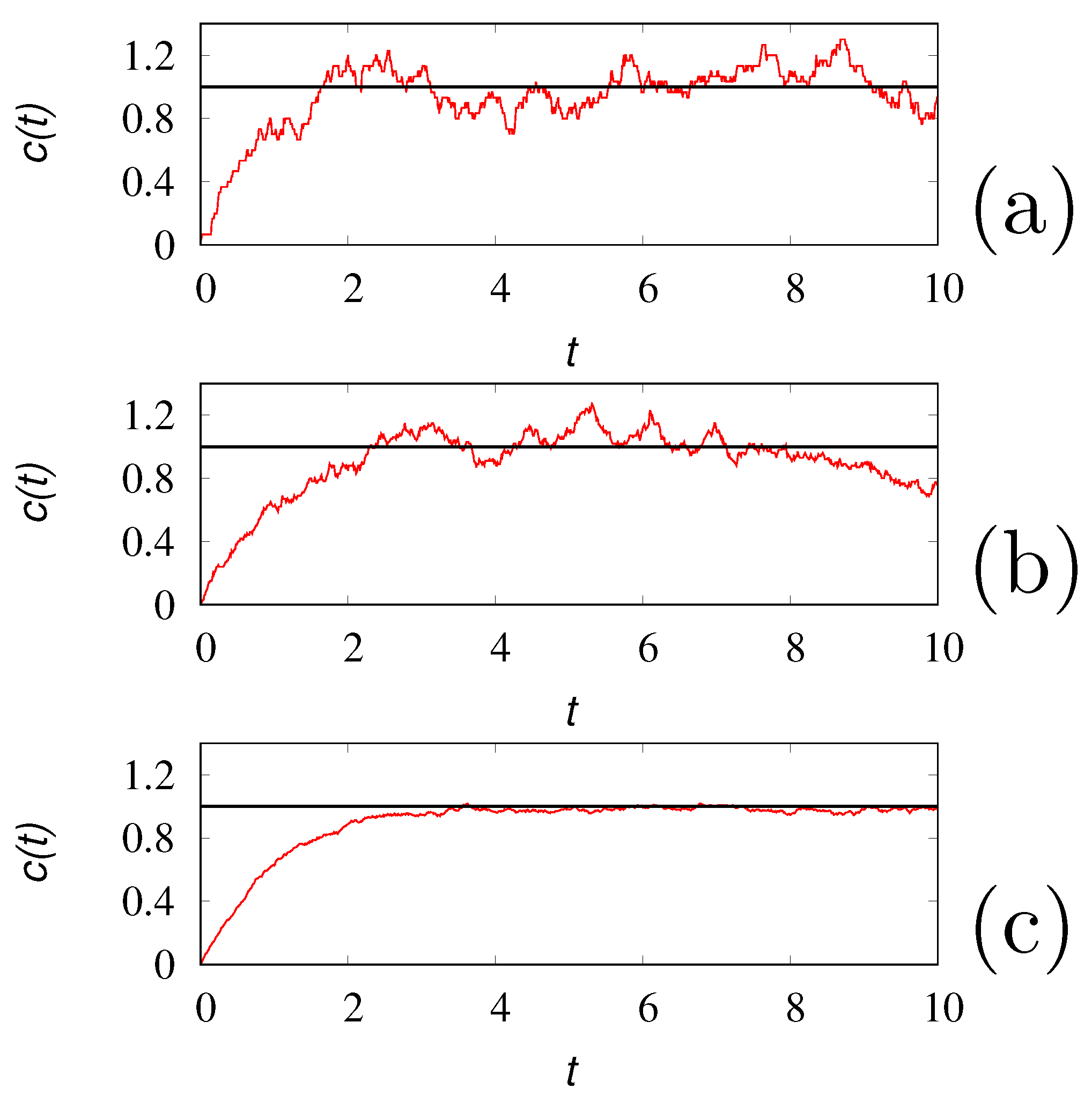
starting from $N\left(0\right)=0$. Figure 3 depicts several realizations of the tank-loading process, obtained by discretizing eq. (17) with a time step $\mathsf{\Delta }t={10}^{-3}$.

This approach can be extended to the analysis of chemical kinetics in flow systems (specifically microfluidic devices) for aggregation and gelation processes, that possess persistent chemical fluctuations, see e.g. [46].

Despite the simplicity of eqs. (16) or (17), this process permits to highlight the role of $N_g$, that can be referred to as the granularity number, and the way stochastic models of chemical reactions can be fruitfully applied. Indeed, there is a two-fold use of the stochastic formulation of chemical kinetic schemes. The first refers to a chemical reacting system involving a small number of molecules, and in this case $N_g$ represents the effective number of molecules present in the system. The other is to use stochastic algorithms for simulating reacting systems as an alternative way, sometimes more efficient, with respect to the solution of the corresponding mean-field equations. In the latter case, the granularity number $N_g$ represents essentially a computational parameter, tuning the intensity of the fluctuations. 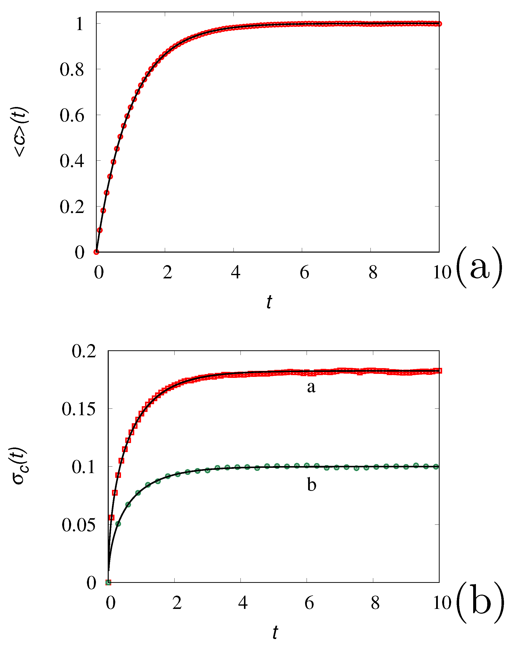Two choices are then possible: (i) $N_g$ can be chosen large enough, in order to obtain from a single realization of the process an accurate approximation of the mean-field behavior, or (ii) it can be chosen small enough in order, to deal with extremely fast simulations of a single realization of the process, that could be averaged over a statistically significant number of realizations in due time. These two choices are depicted in Figure 3 (panel c), choosing $N_g={10}^3$, and in Figure 4 panel (a) obtained for $N_g=30$. Of course, the latter approach is valid as long as the low-granularity (low values of $N_g$) does not influence the qualitative properties of the kinetics.

The second (computational) use of stochastic simulations of chemical kinetics requires a further discussion. At a first sight, it may appear that any stochastic simulation would be computationally less efficient than the solution of the corresponding mean-field equations. This is certainly true for classical chemical reaction schemes in a perfectly mixed system, for which the mean-field model reduces to a system of ordinary differential equations for the concentrations of the reactants. But there are kinetic problems e.g., associated with the growth of microorganisms and eukaryotic cell lines in bioreactors (these growth phenomena, are indeed amenable to a description in terms of equivalent chemical reactions), the mean-field model of which is expressed in the form of higher-dimensional nonlinear integro-differential equations . For this class of problems, the use of stochastic simulations is the most efficient, if not the only way to achieve a quantitative description of the process, in those cases where the number $n_p$ of internal parameters describing the physiological state of an eukaryotic cell becomes large enough [45]. This case is altogether similar to some transport problems, such as Taylor-Aris dispersion for high Péclet numbers or the analysis of microfluidic separation processes (DLD devices) for which the stochastic simulation of particle motion is far more efficient that the corresponding solution of the corresponding mean-field model expressed in the form of advection-diffusion equations [47,48].

To complete the analysis of the tank-loading problem, the associated CME reads

$$\frac{dp(n,t)}{dt}=D{N}_g\left[p(n-1,t){\eta }_{n-1}-p(n,t)\right]+D\left[(n+1)p(n+1,t)-np(n,t)\right]$$

(18)

where ${\eta }_h=1$ for $h\ge 0$ and ${\eta }_h=0$ otherwise. It follows that $\langle c\rangle \left(t\right)=c_0{\sum }_{n=1}^{\infty }np(n,t)/N_g$ satisfies identically the mean-field equation (due to the linearity of the problem), while the variance ${\sigma }_c\left(t\right)$, with ${\sigma }_c^2\left(t\right)=c_0^2{\sum }_{n=1}^{\infty }{n}^{2}p(n,t)/N_g^2-{\left(c_0{\sum }_{n=1}^{\infty }np(n,t)/N_g\right)}^2$, satisfies the equation

$$\frac{d{\sigma }_c^2}{dt}=-2D{\sigma }_c^2+D\left(\frac{1}{N_g}+\frac{\langle c\rangle }{N_g}\right)$$

(19)

Figure 4 panel (b) compares the results of stochastic simulations against the solutions of eq. (19) for two values of $N_g$.

The above approach can be extended to any system of nonlinear reaction schemes involving unimolecular and bimolecular reaction, and in the presence of slow/fast kinetics. The structure of the reaction mechanism can be arbitrarily complicated without adding any further complexity (other than purely notational) in the formulation of the stochastic evolution expressed in terms of number of molecules. The only practical issue, is that the number of different families of stochastic processes grows with the number of elementary reactive processes considered. For instance, in the case of the substrate-inhibited Michaelis-Menten kinetics

$$\begin{array}{c}\hfill E+S\underset{k_{-1}}{\stackrel{k_1}{\rightleftharpoons }}ES\\ \hfill ES\stackrel{k_2}{\to }E+P\\ \hfill ES+S\underset{k_{-3}}{\stackrel{k_3}{\rightleftharpoons }}ESS\end{array}$$

(20)

there are five reactive processes (five channels in the language of the Gillespie algorithm) and consequently five families of counting processes $\left\{{\chi }_{i_h}^{\left(h\right)}(t,·)\right\}$, $h=1,\cdots ,5$, should be introduced, so that the formulation of the discrete stochastic dynamics reads

$$\begin{array}{ccc}\hfill \frac{d{N}_S\left(t\right)}{dt}& =& -\sum _{i=1}^{N_S\left(t\right)}\frac{d{\chi }_i^{\left(1\right)}(t,{\tilde{k}}_1{N}_E\left(t\right))}{dt}+\sum _{j=1}^{N_{ES}\left(t\right)}\frac{d{\chi }_j^{\left(2\right)}(t,k_{-1})}{dt}\hfill \\ \hfill \frac{d{N}_E\left(t\right)}{dt}& =& -\sum _{i=1}^{N_S\left(t\right)}\frac{d{\chi }_i^{\left(1\right)}(t,{\tilde{k}}_1{N}_E\left(t\right))}{dt}+\sum _{j=1}^{N_{ES}\left(t\right)}\frac{d{\chi }_j^{\left(2\right)}(t,k_{-1})}{dt}+\sum _{h=1}^{N_{ES}\left(t\right)}\frac{d{\chi }_h^{\left(3\right)}(t,k_2)}{dt}\hfill \\ \hfill \frac{d{N}_{ES}\left(t\right)}{dt}& =& \sum _{i=1}^{N_S\left(t\right)}\frac{d{\chi }_i^{\left(1\right)}(t,{\tilde{k}}_1{N}_E\left(t\right))}{dt}-\sum _{j=1}^{N_{ES}\left(t\right)}\frac{d{\chi }_j^{\left(2\right)}(t,k_{-1})}{dt}-\sum _{h=1}^{N_{ES}\left(t\right)}\frac{d{\chi }_h^{\left(3\right)}(t,k_2)}{dt}\hfill \\ & -& \sum _{k=1}^{N_S\left(t\right)}\frac{d{\chi }_k^{\left(4\right)}(t,{\tilde{k}}_3{N}_{ES}\left(t\right))}{dt}+\sum _{l=1}^{N_{ESS}\left(t\right)}\frac{d{\chi }_l^{\left(5\right)}(t,k_{-3})}{dt}\hfill \\ \hfill \frac{d{N}_{ESS}\left(t\right)}{dt}& =& \sum _{k=1}^{N_S\left(t\right)}\frac{d{\chi }_k^{\left(4\right)}(t,{\tilde{k}}_3{N}_{ES}\left(t\right))}{dt}-\sum _{l=1}^{N_{ESS}\left(t\right)}\frac{d{\chi }_l^{\left(5\right)}(t,k_{-3})}{dt}\hfill \\ \hfill \frac{d{N}_P\left(t\right)}{dt}& =& \sum _{h=1}^{N_{ES}\left(t\right)}\frac{d{\chi }_h^{\left(3\right)}(t,k_2)}{dt}\hfill \end{array}$$

(21)

equipped with the initial conditions $c_S\left(0\right)=c_{S,0}$, $c_E\left(0\right)=c_{E,0}$, $c_{ES}\left(0\right)=c_{ESS}\left(0\right)=c_P\left(0\right)=0$. Observe that for the bimolecular steps we have used a number-dependent rate coefficient.

The granularity number $N_g$ can be fixed, so that

$$N_S\left(0\right)=\left[c_{S,0}{N}_g\right],N_{E,0}=\left[c_{E,0}{N}_g\right]$$

(22)

where $\left[\xi \right]$ indicates the integer part of $\xi$, thus defining the relation between $N_{\alpha }\left(t\right)$ and $c_{\alpha }\left(t\right)$, namely $c_{\alpha }\left(t\right)=N_{\alpha }\left(t\right)/N_g$, $\alpha =S,E,ES,ESS,P$. This implies also that the effective rate parameters entering the discrete stochastic evolution equation (21), and associated with the two bimolecular reactive steps, are given by ${\tilde{k}}_1=k_1/N_g$, and ${\tilde{k}}_3=k_3/N_g$.

Consider the case $k_{-1}=k_2=k_3=k_{-3}=1$, $c_{S,0}=4$, $c_{E,0}=0.1$. In this case the quasi steady-state approximation of the $c_{ES}$-$c_S$ curve (representing the slow manifold of the kinetics) takes the expression

$$c_{ES}=\frac{c_{E,0}{c}_S}{K_M+c_S+\beta c_S^2},K_M=\frac{k_{-1}+k_2}{k_1},\beta =\frac{k_{-3}}{k_3}$$

(23)

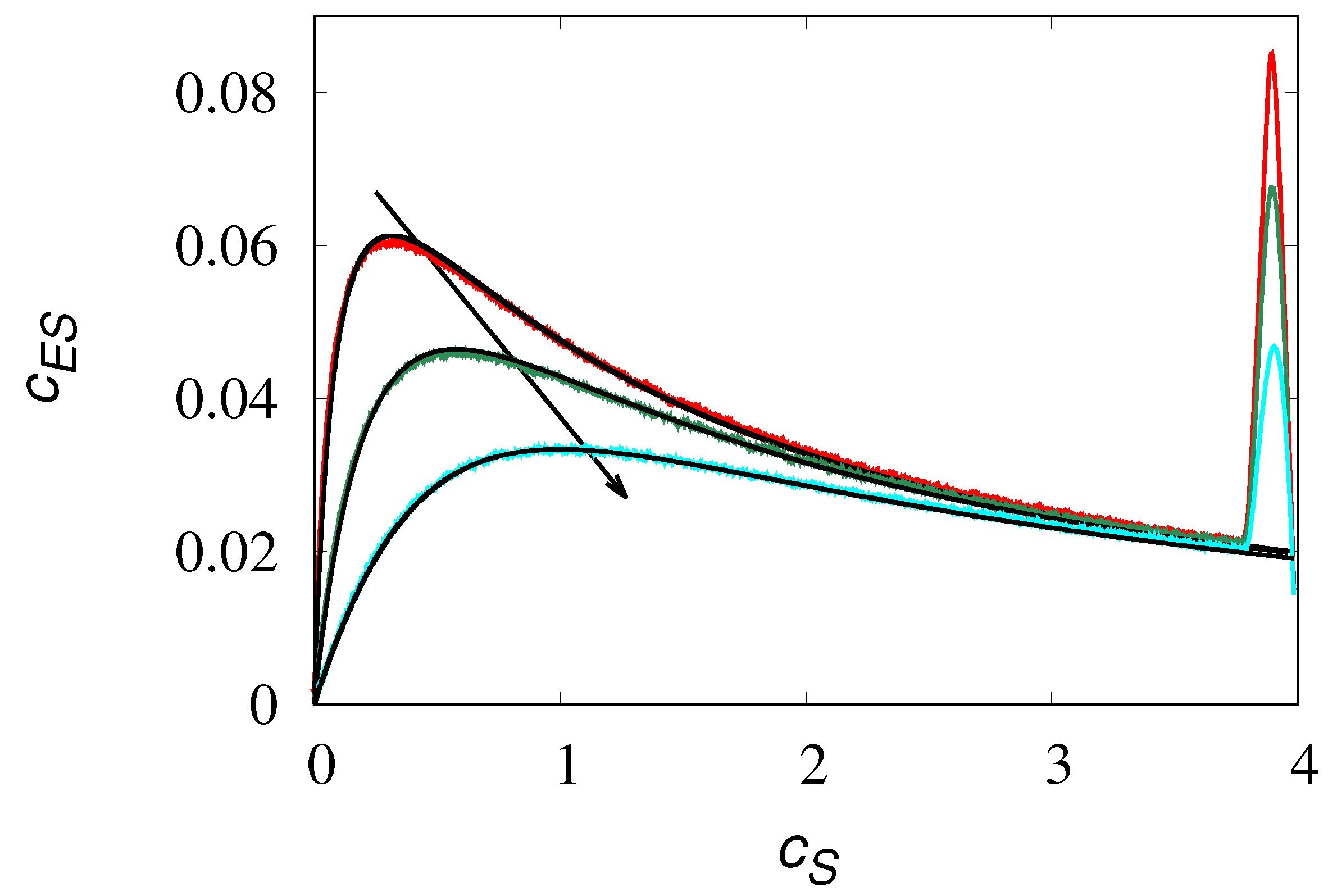
Figure 5 depicts the $c_{ES}$-$c_S$ graph obtained from a single realization of the stochastic process eq. (21) at several values of $k_1$ so as to modify the Michaelis-Menten constant $K_M$ for a value $N_g={10}^6$ of the granularity number.

Apart from the initial transient giving rise to an overshot in the values of $c_{ES}$ near $c_S\simeq c_{S,0}$, the dynamics rapidly collapses towards the slow manifold and the stochastic simulations at high $N_g$-value provide a reliable description of the mean-field behavior starting from a single stochastic realization.

5. Extensions: clustering of liquid molecules and velocity fluctuations

The mechanism controlling fluctuations in chemical kinetics can be extended to any kind of chemical physical process in which some properties change discontinuously as a consequence of elementary events. This is the case of aggregation/fragmentation phenomena, adsorption and quantum transitions. In this Section we consider a particular case of aggregation, related to the clustering of molecules in liquids such as water due to weak interactions [49,50,51]. The dynamics of creation and destruction of clusters is controlled by weak forces and hydrogen-bond formation. This determines that the effective mean square velocity of water molecules at constant temperature T is not $k_{B}T/m$ (where m is the mass of a water molecule), but rather $\langle v^2\rangle =k_{B}T/m_{\mathrm{eff}}$, with $m_{\mathrm{eff}}>m$, due to clustering. Therefore, cluster kinetics has a relevant effect not only at a molecular level but also on the thermodynamic and transport properties of the solution.

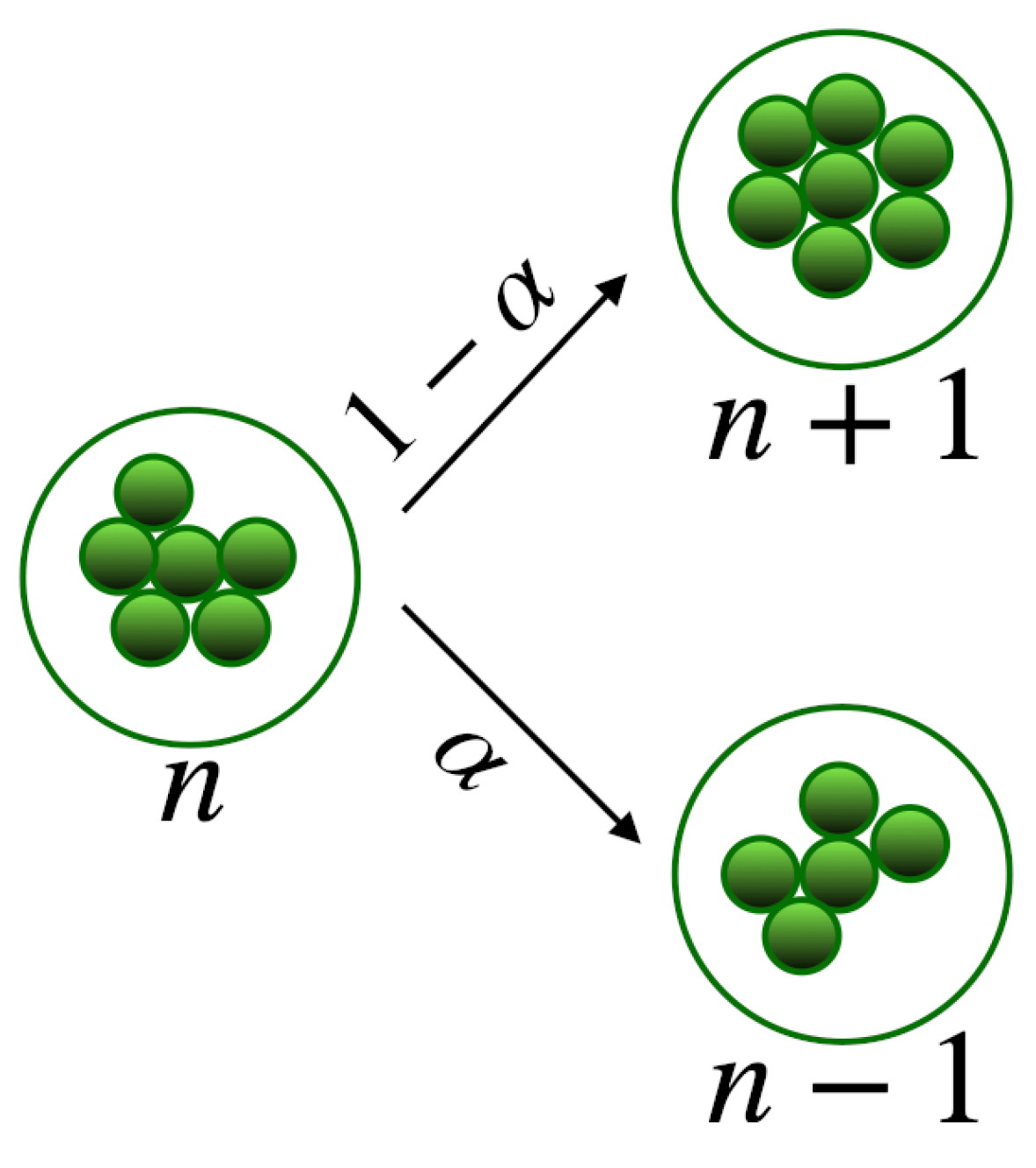
Let us assume that in the clustering process only one molecule at a time is either incorporated in a cluster or eliminated from it, as depicted in Figure 6, and that clustering dynamics can be regarded as linear, i.e. with rates independent of the concentration of the molecules. The process is defined by two parameters: the rate $\lambda$ at which a cluster undergoes a transition, and the probability $\alpha$ that this transition corresponds to the acquisition of another molecule. Moreover, let us assume that there is a maximum number of molecules N above which no cluster can be formed. Therefore, for each molecule, we can define a state variable ${\sigma }_h\left(t\right)$, attaining values $1,2,\cdots ,N$, specifying the cluster-state of the molecule: ${\sigma }_h\left(t\right)$ corresponds to the size of the cluster to which the molecule belongs to. The dynamics of the cluster formation is thus described by the stochastic evolution equation for ${\sigma }_h\left(t\right)$,

$$\frac{d{\sigma }_h\left(t\right)}{dt}=\frac{d{\chi }^{\left(1\right)}(t,{\lambda }_{{\sigma }_h\left(t\right)}^{\left(1\right)})}{dt}-\frac{d{\chi }^{\left(2\right)}(t,{\lambda }_{{\sigma }_h\left(t\right)}^{\left(2\right)})}{dt}$$

(24)

where

$$\begin{array}{ccc}\hfill {\lambda }_1^{\left(1\right)}& =& \lambda ,{\lambda }_h^{\left(1\right)}=\lambda (1-\alpha )(1-{\delta }_{h,N}),h=2,\cdots ,N\hfill \\ \hfill {\lambda }_h^{\left(2\right)}& =& \lambda \alpha (1-{\delta }_{h,1}),h=1,\cdots ,N-1,{\lambda }_N^{\left(2\right)}=\lambda \hfill \end{array}$$

(25)

Indicating with $P_h\left(t\right)$, $h=1,\cdots ,N$ the probability that a molecule belongs at time t to a cluster of h elements, we have

$$\begin{array}{ccc}\hfill \frac{d{P}_1}{dt}& =& -\lambda P_1+\alpha \lambda P_2\hfill \\ \hfill \frac{d{P}_2}{dt}& =& \lambda P_1-\lambda P_2+\alpha \lambda P_3\hfill \\ \hfill \frac{d{P}_k}{dt}& =& (1-\alpha )\lambda P_{k-1}-\lambda P_k+\alpha \lambda P_{k+1},k=3,\cdots ,N-2\hfill \\ \hfill \frac{d{P}_{N-1}}{dt}& =& (1-\alpha )\lambda P_{N-1}-\lambda P_{N-1}+\lambda P_N\hfill \\ \hfill \frac{d{P}_N}{dt}& =& (1-\alpha )\lambda P_{N-1}-\lambda P_N\hfill \end{array}$$

(26)

Equations (26) represent a particular case of the Becker-Döring nucleation kinetics [52,53,54], the matrix representation of which attains the form

$$\frac{d{P}_k}{dt}=\sum _{j=1}^N{\mathsf{\Lambda }}_{k,j}{P}_j,k=1,\cdots ,N$$

(27)

The stationary equilibrium distribution $P_k^{*}$ is given by

$$P_k^{*}=C,P_k^{*}=C\frac{{(1-\alpha )}^{k-2}}{{\alpha }^{k-1}},k=2,\cdots ,N_1,P_N^{*}=C\frac{{(1-\alpha )}^{N-2}}{{\alpha }^{N-2}}$$

(28)

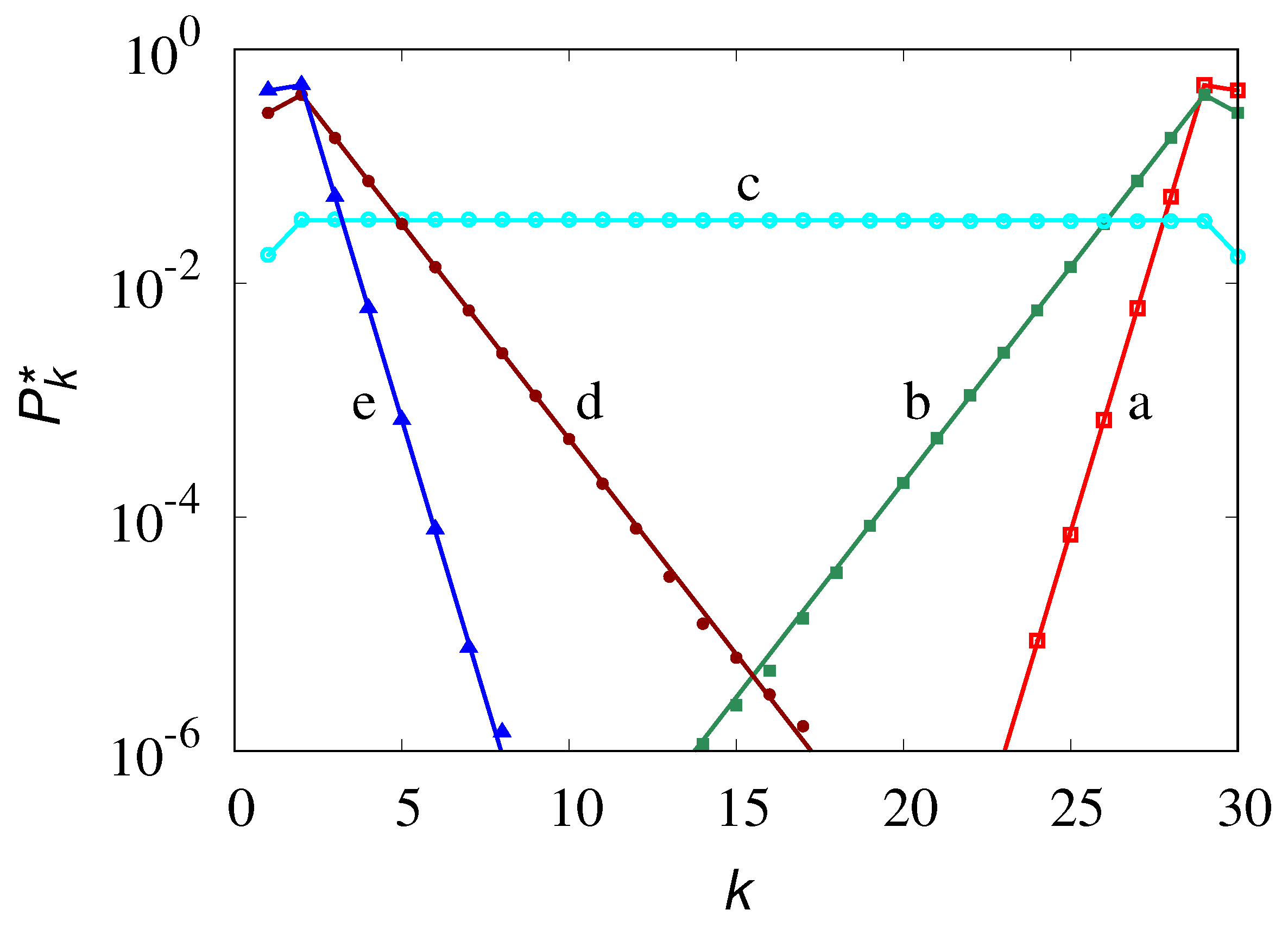
where C is the normalization constant such that ${\sum }_{k=1}^N{P}_k^{*}=1$. Figure 7 depicts the comparison between stochastic simulations using an ensemble of $N_p={10}^5$ realizations of eq. (24) and the steady-sate solution eq. (28).

The microscopic phenomenon of coalescence impacts on macroscopic transport properties, as the motion of clusters is controlled by its size, both as regards inertial (mass) and hydrodynamic interactions (friction factor). If we indicate with $m_k$ and ${\eta }_k$ the mass and the friction factor of a cluster of k molecules, the velocity $v_k$ of a k-cluster satisfies the Langevin equation

$$m_{k}d{v}_k=-{\eta }_k{v}_{k}dt+\sqrt{2k_{B}T{\eta }_k}d{w}_k\left(t\right)$$

(29)

where $w_k\left(t\right)$, $k=1,\cdots ,N$ are a family of Wiener processes independent of each other. We use here a scalar representation for the velocity as the vector representation does not add any new physics, making the notation more cumbersome. The masses $m_k$ and the friction factors ${\eta }_k$ depend on k. Since $m_k=mk\sim R_k^3$, where $R_k$ is the gyration radius of the k-cluster, and ${\eta }_k\sim R_k$, we can set

$${\eta }_k={\eta }_0{k}^{1/3}$$

(30)

where ${\eta }_0>0$ is a constant. Let $P_{v,k}(v,t)$ be the joint density function for v and ${\sigma }_i\left(t\right)$ for the generic i-th molecule

$$P_{v,k}(v^{\prime },t)dv=Prob\left[v\left(t\right)\in (v^{\prime },v^{\prime }+dv),{\sigma }_i\left(t\right)=k\right]$$

(31)

The system of partial densities $P_{v,k}(v,t)$ satisfies the family of Fokker-Planck equations

$$\frac{\partial P_{v,k}(v,t)}{\partial t}=\frac{\partial }{\partial v}\left(\frac{{\eta }_{k}v}{m_k}{P}_{v,k}(v,t)\right)+\frac{k_{B}T{\eta }_k}{m_k^2}\frac{{\partial }^2{P}_{v,k}(v,t)}{\partial v^2}+\sum _{j=1}^N{\mathsf{\Lambda }}_{k,j}{P}_j(v,t)$$

(32)

$k=1,\cdots ,N$. The average value of any function $f\left(v\right)$ of the velocity at time t is thus given by

$$\langle f\left(v\left(t\right)\right)\rangle =\sum _{k=1}^N\langle f\left(v_k\left(t\right)\right)\rangle =\sum _{k=1}^N{\int }_{-\infty }^{\infty }f\left(v\right)P_{v,k}(v,t)dv$$

(33)

Of particular interest is the value of $\langle v^2\left(t\right)\rangle$. From eq. (32) it follows that $\langle v_k^2\left(t\right)\rangle$, $k=1,\cdots ,N$, satisfy the equations

$$\frac{d\langle v_k^2\rangle }{dt}=-\frac{2{\eta }_k}{m_k}\langle v_k^2\rangle +\frac{2k_{B}T{\eta }_k}{m_k^2}{P}_k+\sum _{j=1}^N{\mathsf{\Lambda }}_{k,j}\langle v_j^2\rangle$$

(34)

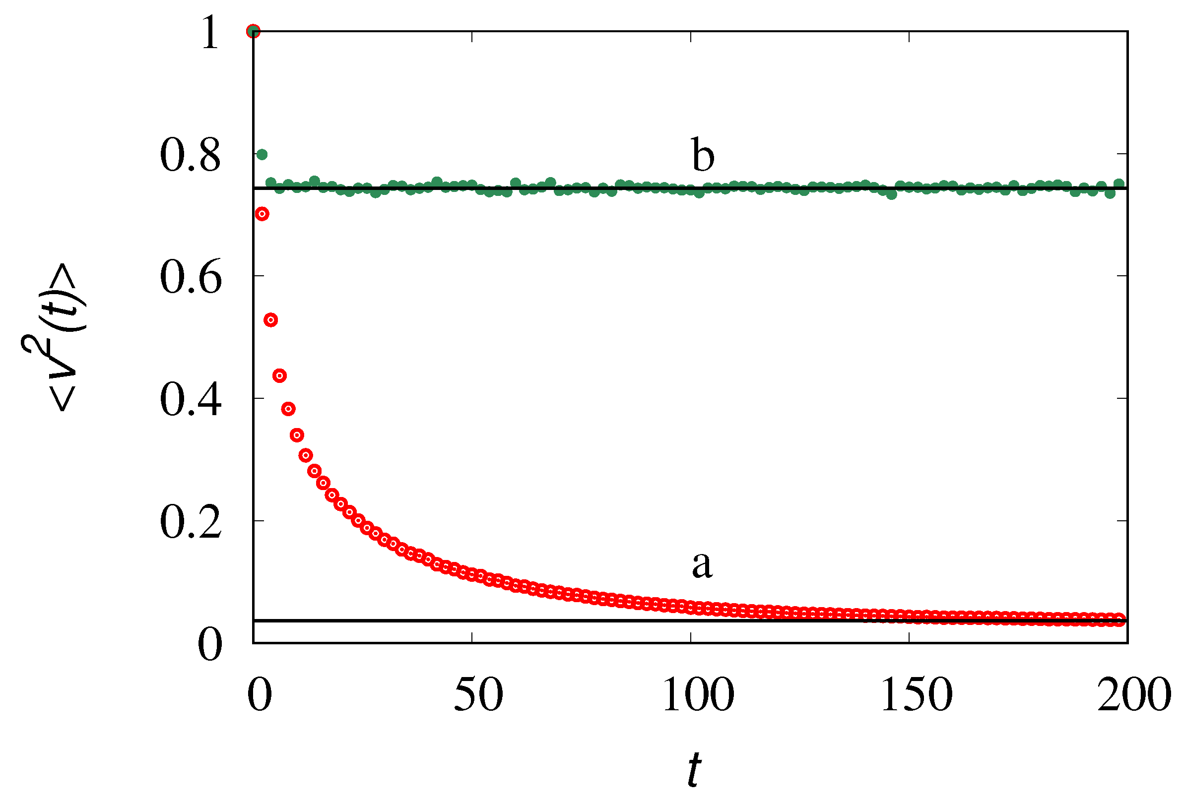
$k=1,\cdots ,N$, where $P_k\left(t\right)$ are the marginal densities with respect to ${\sigma }_i$, solution of eq. (27). Figure 8 depicts the evolution for $\langle v^2\left(t\right)\rangle$ obtained from stochastic simulations with $N_p={10}^5$ elements, initially in the form of single molecules ${\sigma }_i\left(0\right)=1$, $i=1,\cdots ,N_p$, with velocities sampled from the equilibrium distribution. Throughout these simulations we set $N=30$, $k_{B}T$=1 a.u., $m=1$ a.u. and ${\eta }_0=1$ a.u., as the values of these parameters can be rescaled out and they do not influence the qualitative properties of the system. Correspondingly, the initial velocities for the molecules are sampled from a normal distribution with zero mean and unit variance. The data depicted in Figure 8 refers to two values of the parameter $\alpha$.

Of major interest are the long-term equilibrium properties, corresponding to the steady solution of eq. (34). The squared velocity variance $\langle v^2\rangle$ is given by the sum of the marginal squared variances

$$\langle v^2\rangle =\sum _{k=1}^N\langle v_k^2\rangle$$

(35)

Set ${\mathsf{\Lambda }}_{k,j}=\lambda {\tilde{\mathsf{\Lambda }}}_{k,j}$, where ${\tilde{\mathsf{\Lambda }}}_{k,j}\sim O\left(1\right)$. Two limit regimes occur. If $\lambda \ll 1$, the recombination term (last term at the r.h.s. of eq. (34)) can be neglected and thus the equilibrium values for the squared velocity variances are given by

$$\langle v_k^2\rangle =\frac{k_{B}T}{m_k}{P}_k^{*},k=1,\cdots ,N$$

(36)

where $P_k^{*}$ are the equilibrium fractions eq. (28). Conversely, if $\lambda \gg 1$, the recombination term prevails, and the squared partial variances approach the solution of the equation

$$\sum _{j=1}^N{\widehat{\mathsf{\Lambda }}}_{k,j}\langle v_j^2\rangle =0$$

(37)

This means that the $\langle v_k^2\rangle$ should be proportional to the equilibrium fractions

$$\langle v_k^2\rangle =c{P}_k^{*}$$

(38)

where the proportionality constant $c>0$ can be determined by substituting this expression into eq. (34) at steady-state, from which we obtain

$$c=k_{B}T\frac{{\sum }_{k=1}^N\frac{{\eta }_k}{m_k^2}{P}_k^{*}}{{\sum }_{k=1}\frac{{\eta }_k}{m_k}{P}_k^{*}}$$

(39)

Therefore, $\langle v^2\rangle$ attains the two limit values

$$\underset{\lambda \to 0}{lim}\langle v^2\rangle ={\langle v^2\rangle }_0,\underset{\lambda \to \infty }{lim}\langle v^2\rangle ={\langle v^2\rangle }_{\infty }$$

(40)

where

$${\langle v^2\rangle }_0=k_{B}T\sum _{k=1}^N\frac{P_k^{*}}{m_k},{\langle v^2\rangle }_{\infty }=k_{B}T\frac{{\sum }_{k=1}^N\frac{{\eta }_k{P}_k^{*}}{m_k^2}}{{\sum }_{k=1}\frac{{\eta }_k{P}_k^{*}}{m_k}}$$

(41)

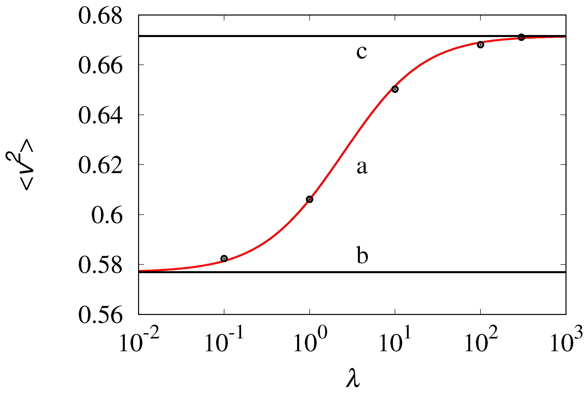
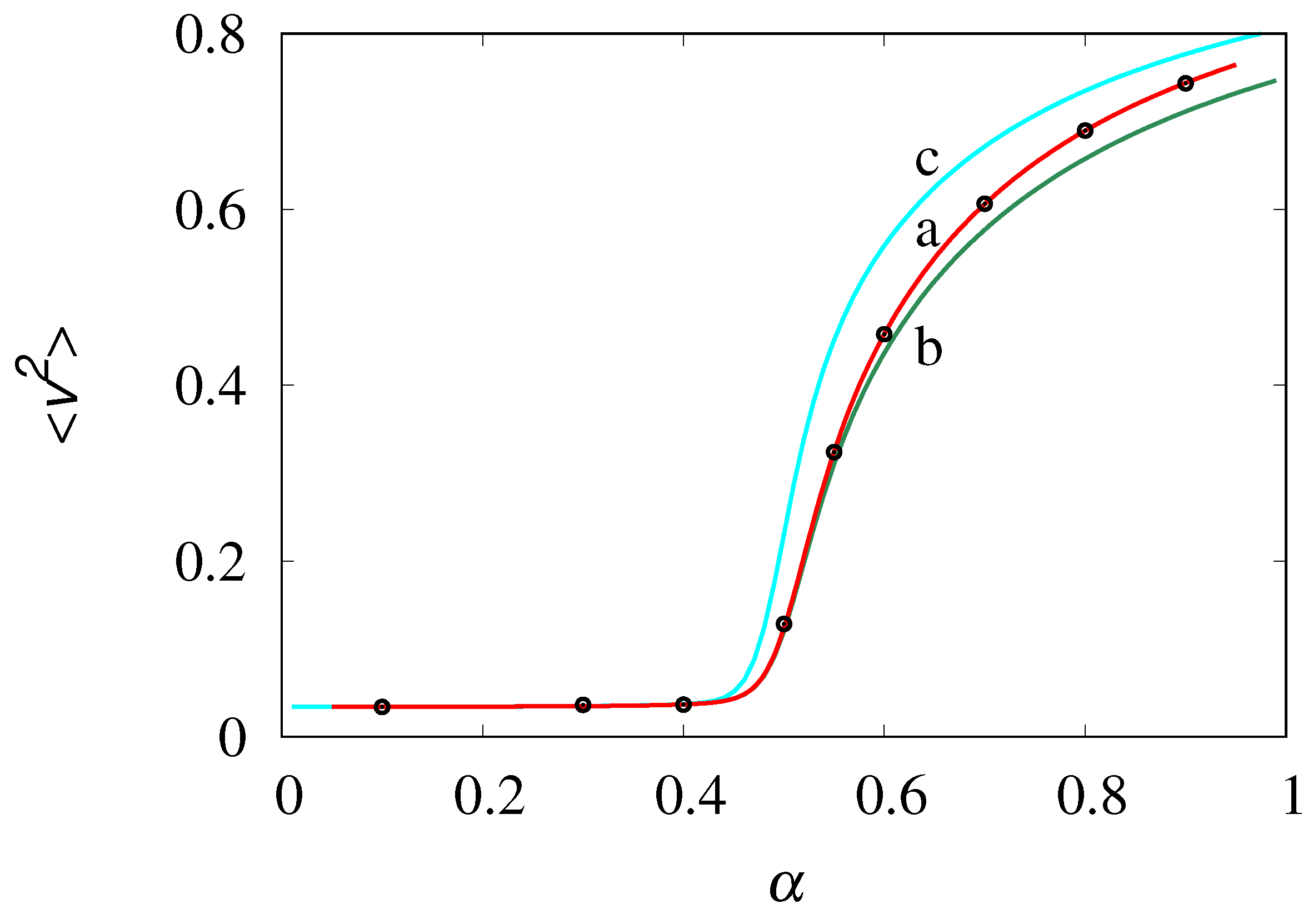
The occurrence of these two limit regimes is depicted in Figure 9 and Figure 10.

Observe that for low values of $\alpha$ ($\alpha \le 0.4$) the influence of the rate $\lambda$ on the intensity of the velocity fluctuations is practically negligible, and ${\langle v^2\rangle }_{\infty }\simeq {\langle v^2\rangle }_0$. This condition corresponds to the formation of very large clusters, having the size of the order of N. Much higher variability occurs for values of $\alpha >0.5$ approaching $\alpha =1$ as this corresponds to the most active kinetic regime with the formation of smaller clusters of the size of few molecules, in which the value of the rate $\lambda$ plays a leading role in determining the statistical properties of the velocity fluctuations.

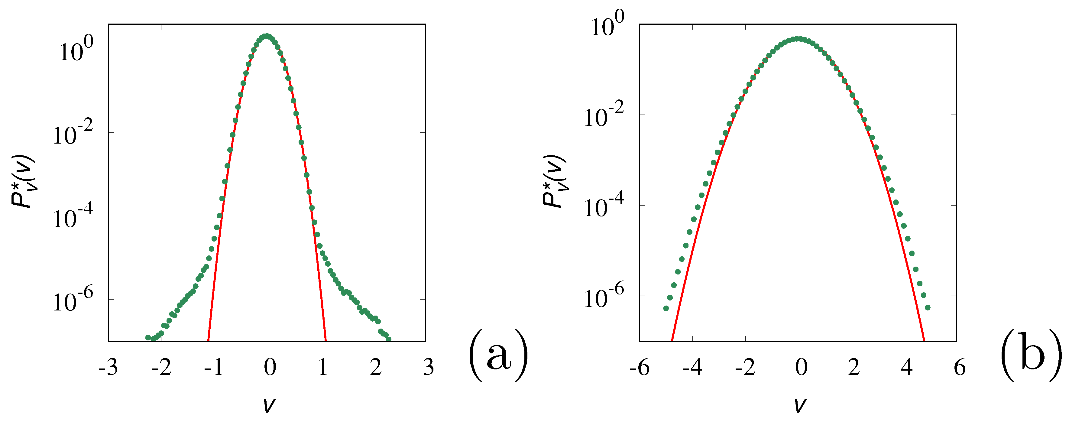
It is also interesting to analyze the velocity density functions $P_v^{*}\left(v\right)$ at equilibrium. Figure 11 depicts the equilibrium densities in these two limit regimes, for values of $\alpha$ below and above the threshold ${\alpha }_c=1/2$.

The results of the stochastic simulations (symbols in Figure 11) refer to a sample of $N_p={10}^6$ realizations. Once the stationary equilibrium conditions have been achieved, the densities are evaluated over a sufficiently wide time window to ensure the estimate of the velocity densities from a sample of about ${10}^{11}$ realizations. This ensures that, at least for the range of $P_v^{*}$-values considered, the velocity statistics is accurate. The solid lines in this figure refer to the Maxwellian (Gaussian) distribution

$$g(v,\sigma )=\frac{1}{2\pi {\sigma }^2}{e}^{-v^2/2{\sigma }^2}$$

(42)

with zero mean and variance ${\sigma }^2={\langle v^2\rangle }_{\mathrm{stoch}.\mathrm{simul}.}$ equal to that obtained from the stochastic simulations. It can be observed that for small $\alpha <1/2$ (panel a), a main Gaussian core occurrs at low velocities, but significant deviations from Gaussianity appear in the high-velocity tails. This is non-surprising as the velocity fluctuations are mainly controlled by the formation of large molecular clusters, and the velocity tails account for the relatively small contribution of these clusters. Conversely, for $\alpha >1/3$ (as in panel (b) at $\alpha =0.9$) a slight, but uniform deviation from the Gaussian profile is observed throughout the whole range of v-values.

Next, consider the particle motion defined by the kinematics

$$d{x}_i=v_{i}dt$$

(43)

While in the analysis developed above the values of m and ${\eta }_0$ were immaterial, so that we set them equal to unity, in the description of particle motion they play a relevant role. Therefore, in the remainder let us assume that m and ${\eta }_0$ attain physical values, which implies for the characteristic dissipation time $t_{\mathrm{diss}}=m/{\eta }_0\ll 1$. Consequently, we can assume in eq. (29), the overdamped approximation even for the larger clusters. This means that eq. (43) becomes

$$d{x}_i=\sqrt{\frac{2k_{B}T}{{\eta }_i}}d{w}_i\left(t\right)$$

(44)

Assuming without loss of generality $x_i\left(0\right)=0$, we have for the mean square displacement

$$\langle x^2\left(t\right)\rangle =2k_{B}T\sum _{k=1}^N\frac{P_k^{*}}{{\eta }_k}t$$

(45)

providing, for the effective diffusion coefficient D the expression

$$D=k_{B}T\sum _{k=1}^N\frac{P_k^{*}}{{\eta }_k}=k_{B}T\langle {\eta }^{-1}\rangle$$

(46)

The latter expression for D should be compared with the effective friction factor $\langle \eta \rangle$,

$$\langle \eta \rangle =\sum _{k=1}^N{\eta }_k{P}_k^{*}$$

(47)

From the comparison of eqs. (46)-(47) it is natural to expect that the classical fluctuation-dissipation relation may be violated [55]. The order parameter $\chi$ for this phenomenon is the product

$$\chi =\langle \eta \rangle \langle {\eta }^{-1}\rangle$$

(48)

as $D\langle \eta \rangle =k_{B}T\chi$, and it should be strictly equal to 1 if the classical fluctuation-dissipation relation is verified. Observe that the averages entering eqs. (46)-(47) are evaluated for the equilibrium cluster distribution $P_k^{*}$.

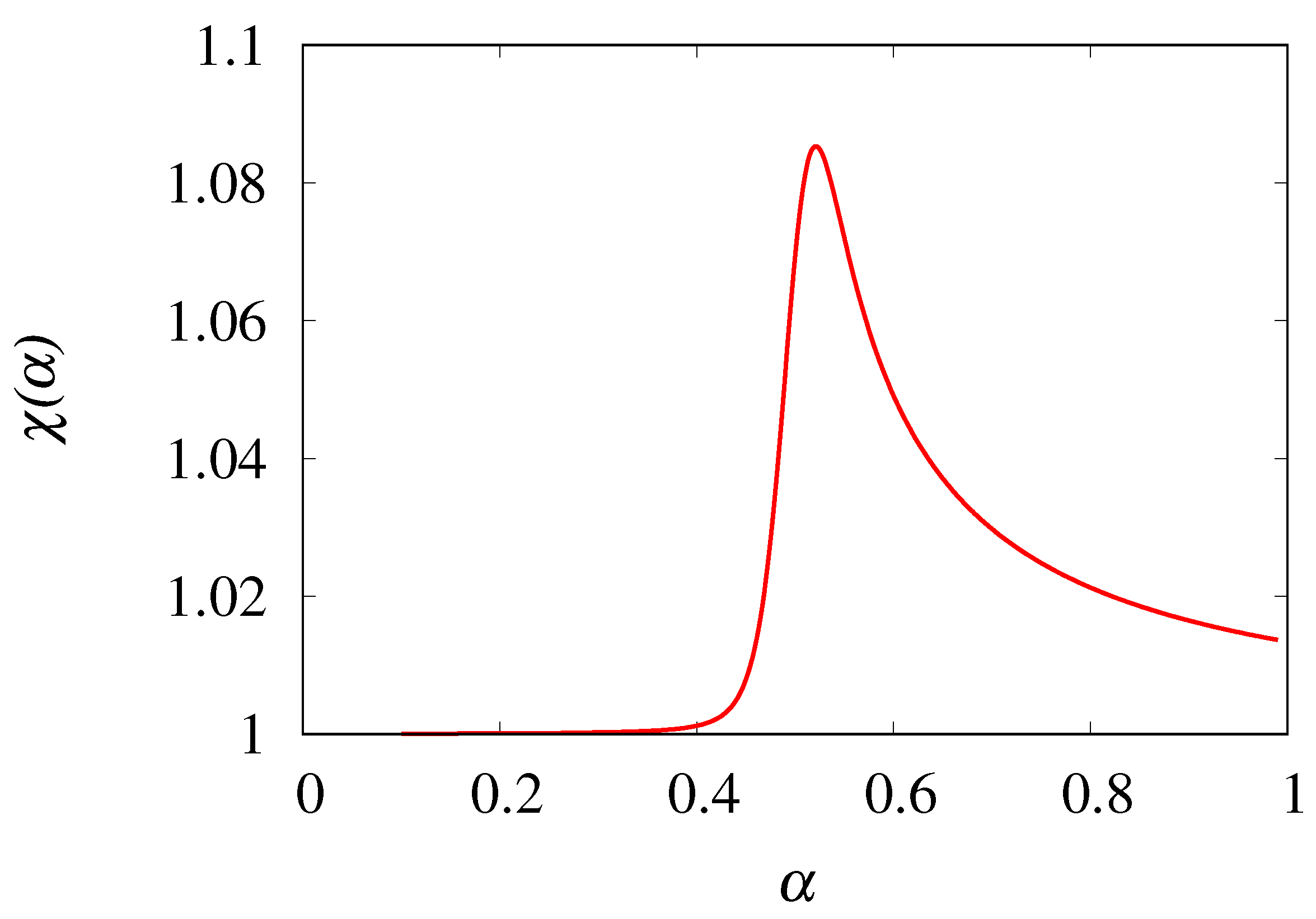
Figure 12 depicts the behavior of $\chi \left(\alpha \right)$ vs $\alpha$ for a maximum cluster size $N=30$. The order parameter is practically equal to 1 for small values of $\alpha$, and the main departure from the fluctuation-dissipation relation (albeit of relative small entity, $|\chi -1|<0.1$), occurs near the critical point ${\alpha }_c=1/2$. This result indicates how microscopic phenomena, such as coalescence, may impact on macroscopic thermodynamic and transport properties, and that it is possible to provide simple and efficient stochastic modelling of them, accounting for the elementary transitions occurring at the molecular level.

6. Radiative interactions and thermalization

Chemical reaction kinetics and quantum transitions can be treated stochastically with the same Markovian setting, once the transition rates are defined starting from the microscopic physics of the elementary events. This is analyzed in detail in [56] to which the reader is referred for further details.

It is important to stress in this context, similarly to the case of coalescence dynamics analyzed in the previous Section, the influence of radiative processes on transport properties. It is well known that the electromagnetic field carries momentum, and consequently it is able to interact “at a mechanical level” with massive bodies, i.e. influencing their momentum dynamics (equations of motion). This problem has been analyzed in detail by Einstein [57], (the English translation can be found in [58], see also the discussion [59,60]), showing that, if a molecular system composed of identical molecules of mass m, and possessing an internal quantized energy structure, amenable to radiative transitions (i.e. absorption and emission of energy quanta), interacts with equilibrium thermal radiation at temperature T, the resulting momentum transfer due to photon kicks and molecular recoil effects determines statistically a squared velocity variance equal to $\langle v^2\rangle =k_{B}T/m$ (componentwise), consistently with the kinetic theory.

This result is of the highest physical importance as it indicates that radiative interactions at the molecular level determine the thermalization of the system independently of other mechanical interactions (such as binary molecular collisions), which possibly may speed up the thermalization process, but not modify its outcome (for the simple reason that binary elastic collisions preserve the sum of the squared norm of velocities of the colliding particles).

The stochastic dynamics of this process has been analyzed in [56]. Due to the impulsive nature of the radiative events, at least in a semiclassical description, momentum-transfer dynamics can be represented by means of an impulsive Langevin equation

$$m\frac{d\mathbf{v}}{dt}=\left(-\eta \mathbf{v}+\mathbf{b}\right)\frac{d\chi (t,\lambda )}{dt}$$

(49)

where $\chi (t,\lambda )$ is a Poisson counting process with transition rate $\lambda$, accounting for the stochasticity and for the frequency of radiative events, $\mathbf{b}=b\mathbf{r}$, where $b=h\nu /c$ the momentum of the photon ($\nu =(E_2-E_1)/h$ is the resonant frequency of the transition between the energy levels $E_1$ and $E_2>E_1$, h the Planck constant, and c the light speed in vacuo), $\mathbf{r}$ a random unit vector, uniformly distributed on the surface of the unit sphere (as thermal radiation is here considered), and $\eta$ the radiative friction factor, possessing the physical dimension of a mass.

Integrating eq. (49) between the occurrence of a radiative event, we have

$${\mathbf{v}}^{\prime }=\alpha \mathbf{v}+\frac{b(1-\alpha )\mathbf{r}}{\eta }$$

(50)

where $\mathbf{v}$ and ${\mathbf{v}}^{\prime }$ are the velocities before and after the event, $\alpha =e^{-\eta /m}$. The parameter $\alpha$ and $\eta$ are related to each other by a radiative fluctuation-dissipation relation [56]

$$3\frac{k_{B}T}{m}(1-{\alpha }^2)=\frac{b^2{(1-\alpha )}^2}{{\eta }^2}$$

(51)

Also in this case, it is interesting to analyze the effects of this microscopic process on the transport properties, using the parameter $\alpha \in (0,1)$ as the quantity controlling radiative dissipation. If $\alpha$ is close to 1, and this physically occurs at “high” temperatures, above ${10}^{-5}$-${10}^{-6}$ K, the resulting velocity density functions are of Gaussian shape, consistently with the Maxwellian theory. 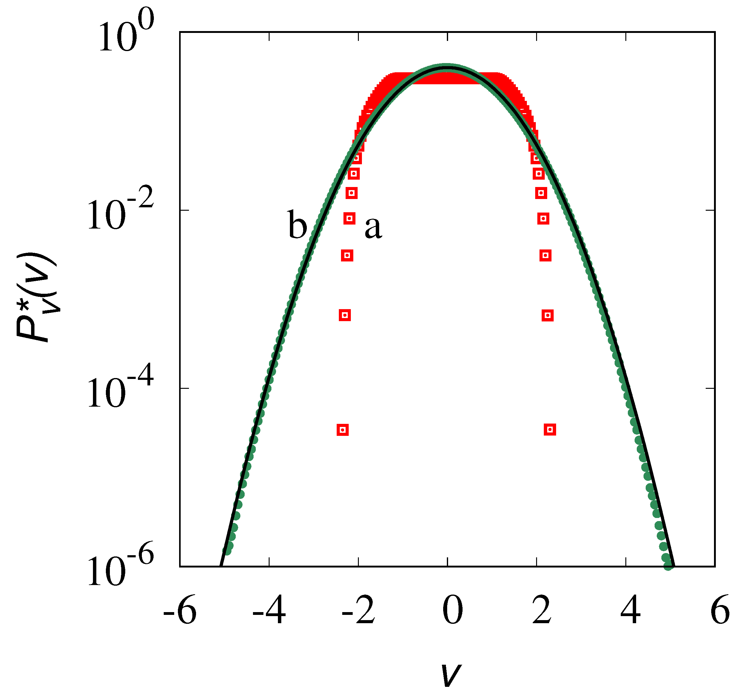Conversely, at very low temperatures, say below ${10}^{-6}$ K, $\alpha$ is definitely smaller than 1, and deviations from Gaussian profiles become evident. This is depicted in Figure 13 obtained by simulating an ensemble of ${10}^8$ particles, undergoing the dynamics (50)-(51) with $k_{B}T/m$ set equal to 1 a.u., for two values of $\alpha$, starting from an initially uniform velocity density function, and considering the equilibrium velocity profile $P_v^{*}\left(v\right)$ for a generic component of $\mathbf{v}$.

The analysis of the mechanical effects of radiative interactions is important at least for the following main reasons:

• it provides a simple physical mechanism, beyond the realm of mechanical interactions (collisions) for the thermalization process leading to thermal equilibrium conditions in a molecular system at constant T, where the temperature T is defined by the statistical properties of the incoming radiation;
• it provides a way to model momentum transfer in the presence of a generic out-of-equilibrium radiation, i.e., in the case the photons are not “thermal photons”, but may possess other statistical properties;
• it indicates that Gaussianity in statistical physics is by no mean a fundamental constitutive principle (see e.g. the analysis of the Central Limit Theory addressed in [68]) as regards kinetic variables (velocities), but it results as a consequence of the physical conditions at which commonly we perform experiments. In the case of the radiative processes, this corresponds to temperatures above ${10}^{-5}$-${10}^{-6}$ K;
• consequently, it provides a way to address the thermodynamic and transport features of cold atoms that, as discussed in [61], are characterized by highly anomalous transport and thermodynamic properties.

7. Concluding remarks

The stochastic modelling of chemical reaction kinetics is paradigmatic for a huge variety of chemical physical processes. In this article we have outlined the transition from a purely algorithmic description of these processes to a formal and simple stochastic formulation driven by distributional derivatives of counting processes. The approach proposed:

• shows a direct analogy between chemical reaction kinetics, radiative processes and stochastic formulation of open quantum systems, thus, paving the way for a unified treatment of the interplay between these phenomena, that is particularly important in the field of photochemistry, and in the foundation of statistical physics [56,62];
• can be easily extended to semi-Markov transitions. This is indeed the case of the growth kinetics of eukaryotic microorganisms, the physiological state of which can be parametrized with respect to internal (hidden) parameters such as the age, the cytoplasmatic content, etc.;
• can be easily extended to include transport phenomena. In point of fact, the occurrence of Markovian or semi-Markovian transitions in modeling chemical kinetics is analogous to the transitions occurring in the direction of motion (Poisson-Kac processes, Lévy flights, Extended Poisson-Kac processes) or in the velocity (linearized Boltzmannian schemes) [63,64,65].
• it is closely related to the formulation of stochastic differential equations for the thermalization of athermal system [66], in which the classical mesoscopic description of thermal fluctuations, using the increments of a Wiener process, is replaced by a dynamic model involving the increments of a counting process.

In a broader perspective, we have shown that it is possible to develop a stochastic microscopic event-based theory of chemical physical processes, and derive out of it macroscopic and emergent features. When microscopic processes are considered, Gaussianity for velocity density functions may be violated, as shown in connection with coalescence dynamics and radiative transitions. Although this violation refers to equilibrium property, it is easy to foresee that that this may impact non-equilibrium phenomena as well, indicating the necessity of modifying the classical parabolic paradigm of transport phenomena Gaussian density profiles stem from, by including and accounting for microscopic event-based physical transitions.