Informer Model with Season-Aware Block for Efficient Power Series Forecasting

Preprint

Article

Informer Model with Season-Aware Block for Efficient Power Series Forecasting

Altmetrics

Downloads

143

Views

Comments

Yunlong Cui^*,Zhao Li,

Peng Zhang^*

Yunlong Cui^*,Zhao Li,

Peng Zhang^*

This version is not peer-reviewed

Submitted:

17 December 2023

Posted:

29 December 2023

You are already at the latest version

Alerts

Abstract

With the development of electricity spot markets, accurate electricity load forecasting enables power generation companies to supply the right amount of electricity, Significantly avoid power waste. As a result, time series forecasting in the field of power can bring significant benefits. Previously, the Informer model successfully introduced the Transformer into long time series forecasting(LTSF) by proposing the ProbSparse self-attention mechanism, which solved the inherent problem of high memory complexity in self-attention. Recent research has further demonstrated the potential of the self-attention for mining complex dependencies. However, the limited amount of historical data has become one of the main challenges in applying deep learning techniques to power LSTF tasks. Previous reserches often add a large number of time covariates to provide more information. In this paper, to address this issue, (i) we design a simple but effective Season-aware Block to enhance the model’s ability to mine artificial prior information in temporal covariates; (ii) we conduct experiments using the provincial power data of Zhejiang Province, China, from 2019 to 2022, and our model outperforms other models, achieving a 19 percent MSE relative improvement; (iii) we conduct ablation experiments to assess the efficacy of the Season-aware Block in extracting temporal periodic features. Furthermore, we elucidate the underlying reasons for the effectiveness of both the self-attention mechanism and the Season-aware Block through visualization experiments.

Keywords:

Subject: Computer Science and Mathematics - Artificial Intelligence and Machine Learning

1. Introduction

Time series analysis is a crucial field in data science, with a wide range of applications. Long-term time series forecasting(LSTF) tasks require models to accurately predict future value over a longer time step using limited input length, which necessitates the model’s ability to correctly fit complex, dependencies from limited data, a challenging task indeed.

In recent years, deep learning methods based on the Transformer, such as Informer [1] and Autoformer [3], have frequently set new records in various fields including medicine, finance, infectious disease transmission, weather, transportation and so on. This demonstrates the powerful capability of the self-attention mechanism in fitting complex dependencies [4]. Many studies have shown that Transformer-based models perform well in LSTF tasks, thanks to the excellent ability of the self-attention to learn context-related dependencies. It can detect intricate cycles that are difficult for humans to induce from target data sequences [5].

Figure 1. Different distribution between ground truth and forecasting output from Informer in ElecZJ dataset. (a): power load in Zhejiang Province during China National Day. (b) power load in Zhejiang Province during Labour Day. xlabel:timestep,ylabel:power load value after normalization.

Figure 2. Different structures for different features.

P_{\hat{x}}

is the Input target sequence.

{\hat{x}}^{a}

and

{\hat{x}}^{b}

represents stable static time covariates.

{\hat{x}}^{a}

represent discrete variable, such as holidays, and

{\hat{x}}^{b}

represent continuous variable, such as hours.

{\hat{x}}^{i}

and

{\hat{x}}^{j}

represents complex dynamic covariates. Informer branch is more sensitive to high-frequency and complex features in the input sequence, while Linear is more sensitive to smooth, stable and fixed social cycle features.

Figure 2. Different structures for different features.

P_{\hat{x}}

is the Input target sequence.

{\hat{x}}^{a}

and

{\hat{x}}^{b}

represents stable static time covariates.

{\hat{x}}^{a}

represent discrete variable, such as holidays, and

{\hat{x}}^{b}

represent continuous variable, such as hours.

{\hat{x}}^{i}

and

{\hat{x}}^{j}

However, in power LSTF tasks, the amount of historical and accurate data is limited due to the limited digitalization time of power companies [6]. Taking the real-time electricity consumption data of Zhejiang Province, China from 2019 to 2022 as an example, the data we used only covers a four-year period. Firstly, when the amount of data is insufficient, it’s unreliable to directly mine long-cycle complex dependencies from target data sequences. This is because electricity consumption is influenced by various human factors, such as holidays, major events, and festivals. These accidental factors may only appear once a year in the entire dataset, such as Chinese lunar holidays, flexible working(where weekends are changed to working days), but have a significant impact on electricity consumption. Therefore, it is essential to incorporate artificial prior information during the data preprocessing stage. Secondly, the complex structure of Transformer-based models makes the model need more data to learn human social information [7], such as festivals, holidays, etc, although in data processing we artificially summarized cyclical covariates.

Therefore, as we augment the model with additional artificial cyclical information in the form of covariates, it is essential to design a new structure that enhances the model’s sensitivity to these cyclical patterns. Based on the above motivation, we propose the Informer with Season-aware Block to accomplish the power LSTF task. Our model still follows encoder-decoder structure [1], while adding a linear structure from input to output. Additionally, we have simplified the original structure of the Informer to prevent overfitting. We refer to this linear structure as the Season-aware Block, which shares the same input. This design empowers our model to accurately capture social cyclical information in artificial covariates and intricate dependencies within target sequences. According to the experimental results, the Season-aware Block performs smooth predictions, while the Informer Block fits complex dependencies in historical data that are difficult to generalize and makes high-frequency change predictions. The predictions from both branches are eventually superimposed to form the final result. Extensive experiments demonstrate that this parallel structure breaks the bottleneck of information utilization and significantly improves the model’s prediction accuracy.

2. Related Work

2.1. Models for LSTF

In recent years, the research of deep learning techniques for addressing long time series prediction challenges has seen significant progress. It has evolved from LSTM [8] and TCN [9] to Transformer-based models [10] for long time series. Initially, the Transformer demonstrated exceptional performance in the NLP domain [4], and some research has proven the capability of its self-attention structure in mining complex dependencies. Given the shared characteristic of sequence inputs in both time series prediction and NLP, and the common challenge of accurately modeling complex context dependencies, there has been a recent surge in Transformer-based LSTF solutions.

To mitigate the memory complexity introduced by the self-attention, LogTrans [11] employs log-sparse attention which used an

O (n log 2 n)

self-correlation structure instead of the

O (n^{2})

complexity. Reformer [5] introduced Locality Sensitice Hashing(LSH) attention that reduces the memory complexity of self-attention to

O (n log n)

, and then Informer [1] proposes the ProbSparse self-attention mechanism to achieves the

O (n log n)

complexity. To simultaneously enhance information utilization, Autoformer [3] porposes an Auto-Corrlation mechanism with dependencies discovery and information aggregation at the series level. However, all of these models attempt to extract more information from the target time sequence, while overlooking the crucial aspect of enabling the model to adeptly incorporate artificial prior information from time covariates during training.

2.2. temporal covariates

Time series covariates refer to one or more variables within time series data that are associated with the target variable, providing additional information to improve predictions or estimates of the target variable’s value. In time series analysis, covariates are typically classified into two categories: static covariates and dynamic covariates. Static covariates are variables that remain constant or experience minimal change within the time series and are often related to fixed timestamp information, such as minutes, hours, days, or months. These covariates can help capture fixed patterns related to time, including seasonality and trends. Conversely, dynamic covariates are variables that vary over time and typically correspond to continuously changing external factors, such as weather and GDP. Dynamic covariates can help capture evolving patterns related to time, thereby enhancing the accuracy of predictions.

3. Preliminary

In this section, we provide the power LSTF problem definition. Under the rolling forecasting setting with a window size of n, the input comprises a power sequence

V_{1 : n} = {v_{1}, . . . . . ., v_{n}}

, where

v_{t}

represents the value of power sequence

V

at time t. The task is to predict the values of target sequence

V_{n + 1 : n + m}

with a size of m. In addition to the power sequence, the input includes static covariates

{Xs}_{1 : n + m}^{ks} = {{xs}_{1}^{i}, . . . . . ., {xs}_{n + m}^{i}}_{i = 1}^{ks}

and dynamic covariates

{Xd}_{1 : n}^{kd} = {{xd}_{1}^{j}, . . . . . ., {xd}_{n}^{j}}_{j = 1}^{kd}

. Static covariates are known for the next m time steps before making the prediction, so the input length for static covariates is

n + m

. On the other hand, dynamic covariates are unknown for the next m time steps, so the input length is n.

k s

and

k d

respectively represent the dimensions of static covariates and dynamic covariates. Thus, the power LSTF problem can be defined as:

V_{n + 1 : n + m} = M o d e l (V_{1 : n}, {Xd}_{1 : n}^{kd}, {Xs}_{1 : n + m}^{ks}),

(1)

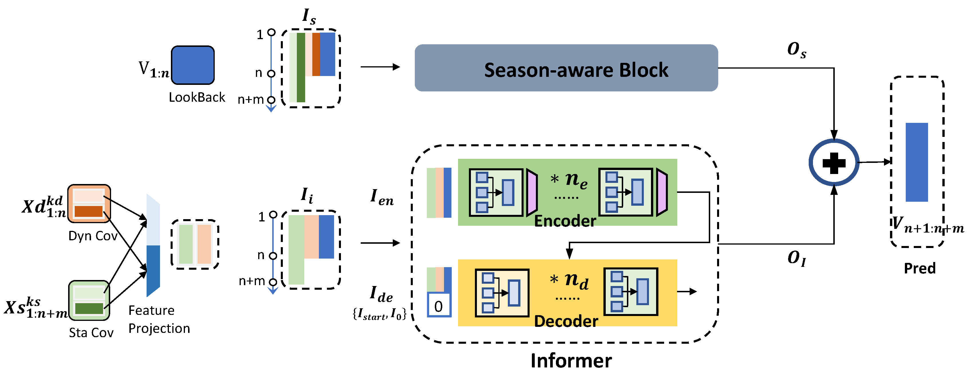
Figure 3. Overview of Informer with Season-aware Block. Our Model consists of Season-aware Block and Informer Block.The input for the Season-aware Block is obtained by directly concatenating the target sequence, static covariates, and dynamic covariates. In contrast, the input of the Informer Block requires the static covariates and dynamic covariates to be processed through Feature Projection before being concatenated with the target sequence. The Informer Block includes

n_{e}

encoders and

n_{d}

decoders. The green squares in both encoder and decoder are Multi-head PorbSparse self-attention Block, the yellow square in decoder is Masked Multi-head ProbSparse self-attention Block, and the purple trapezoid in encoder is Distilling Block.

n_{e}

encoders and

n_{d}

4. Informer with Season-aware Block

In this section, we will provide a detailed introduction to the efficient Informer with Season-aware Block for power LSTF. In our model we add a simple pathway between the input and output to learn the seasonality, particularly in the artificial static time covariates, which we refer to as the Season-aware Block. While retaining the overall structure of the encoder and decoder in the Informer, we have appropriately reduced the number of ProbSparse self-attention layers. This judicious reduction aims to maintain the model’s ability to extract complex periodic dependencies from the data while mitigating the risk of overfitting.

4.1. Model inputs

The input consists of three parts: the Lookback

V

, which constitutes the target time series, along with dynamic covariates

Xd

and static covariates

Xs

. It is worth noting that the Lookback only contains continuous numerical variables, while both dynamic and static covariates include discrete and continuous variables which can be denoted as

Xdd

Xdc

Xsd

, and

Xsc

. Therefore, before feeding into the Informer Block, we perform embedding operations on the discrete variables in both dynamic

Xdd

and static covariates

Xsd

. Additionally, layer normalization is applied to continuous numerical variables

Xdc

and

Xsc

. Then We concatenate them together to form the new dynamic

\bar{Xd}

and static covariates

\bar{Xs}

. Finally, we concatenate the Lookback, dynamic covariates, and static covariates to obtain the final input vector of Informer Encoder

I_{i}

I_{i} = Concat (V, \bar{Xd}, \bar{Xs}),

(2)

Through the above feature projection, we can reduce the feature dimensionality, increase the information density, and transform the discrete variables into continuous ones. This conversion makes it easier for the self-attention structure to fit them. As for the Season-aware Block, we concatenate origin Lookback

V_{1 : n}

, dynamic

X d_{1 : n}^{k d}

and static

X s_{1 : n + m}^{k s}

covariates to obtain input

I_{s}

I_{s} = Concat (V, Xd, Xs) = Concat (V, Xdd, Xdc, Xsd, Xsc),

(3)

4.2. Season-aware Block

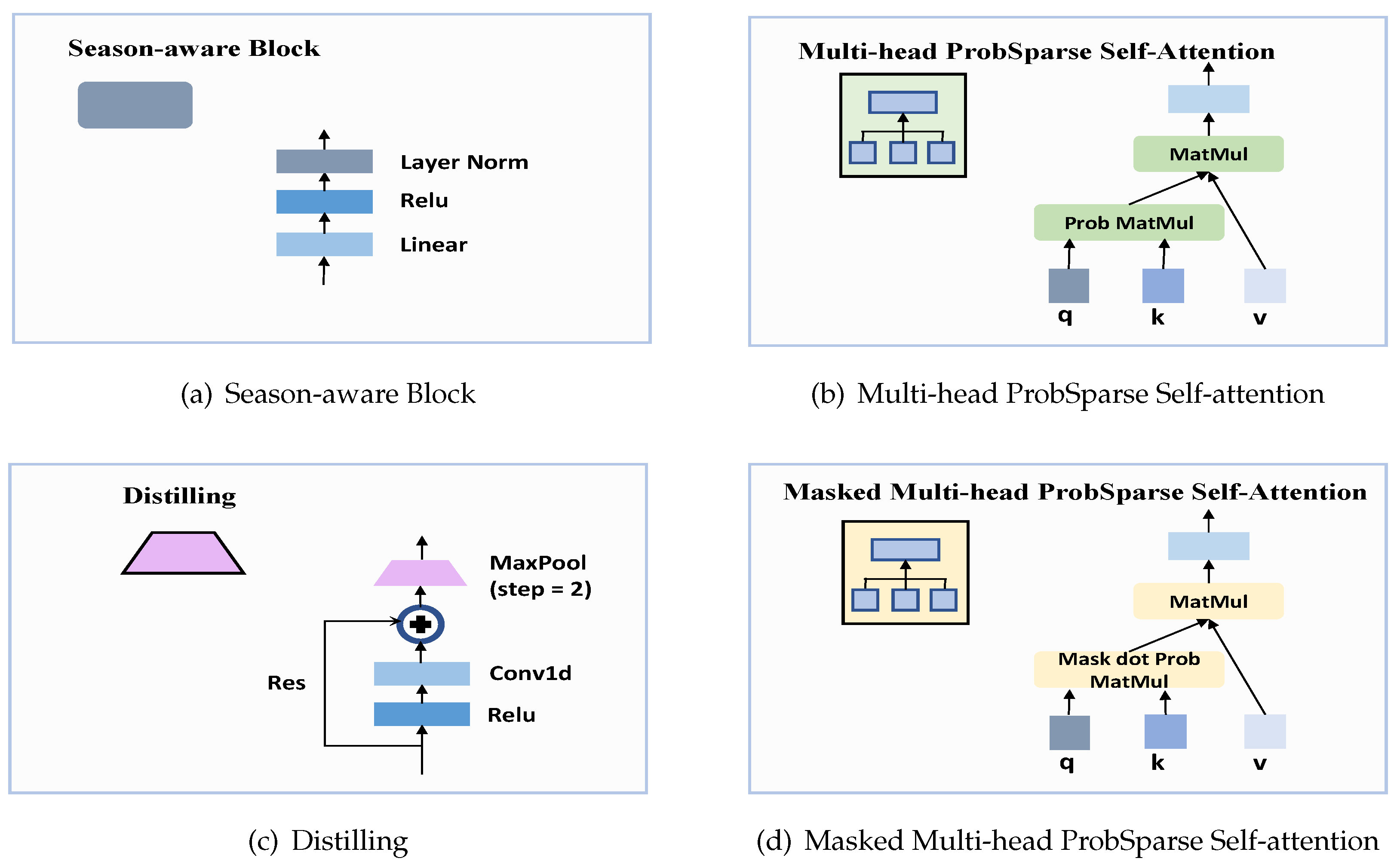
We use the Season-aware Block to enhance the model’s sensitivity to the artificial seasonal information in the time covariates of the input. In Figure 4a, after fully linear layer, we add an ReLU activation and also use layer norm at the output:

O_{s} = Season (I_{s}) = LayerNorm (ReLU (Linear (I_{s}))),

(4)

4.3. Informer

4.3.1. ProbSparse Self-attention

The classic self-attention mechanism, as used in the Transformer, is defined by the function

A (K, Q, V)

Attention (k, Q, V) = Softmax (\frac{{QK}^{T}}{\sqrt{d}}) V,

(5)

Where K, Q, V, and d represent the key, query, value, and input dimension. When using

S o f t m a x (\frac{Q K^{T}}{\sqrt{d}})

to compute the attention weight matrix for an input sequence of length L, the memory complexity is

O (L^{2})

. Subsequently, In the context of long time series forecasting problems, this results in significant computational and memory overhead. So we use ProbSparse self-attention which allow each key to only attend to the u dominant queries [1]:

ProbSparse (k, \bar{Q}, V) = Softmax (\frac{\bar{Q} K^{T}}{\sqrt{d}}) V,

(6)

Where the

\bar{Q}

just contain the top u active queries. Here,

u = c ln L_{Q} = c ln L

and c is called sampling factor hyperparameter for the ProbSparse attention. So the size of

\bar{Q}

c \cdot ln L \cdot d

, and the size of ProbSparse self-attention is

O (L_{K} \cdot ln L_{Q}) = O (L ln L)

To calculate the top u active queries, We use an sparsity measurement

M (q_{i}, K)

to assess the importance of

q_{i}

which is defined as [1]:

M (q_{i}, K) = max {\frac{q_{i} K^{T}}{\sqrt{d}}} - mean {\frac{q_{i} K^{T}}{\sqrt{d}}} = {max}_{j = 1}^{L_{k}} {\frac{q_{i} k_{j}^{T}}{\sqrt{d}}} - \frac{1}{L_{k}} \sum_{j = 1}^{L_{k}} \frac{q_{i} k_{j}^{T}}{\sqrt{d}},

(7)

We only need to randomly sample

v = c \cdot ln L_{K}

dot product pairs to compute the approximation of

M (q_{i}, K)

\bar{M} (q_{i}, \bar{K})

\bar{M} (q_{i}, \bar{K}) = max {\frac{q_{i} {\bar{K}}^{T}}{\sqrt{d}}} - mean {\frac{q_{i} {\bar{K}}^{T}}{\sqrt{d}}} = {max}_{j = 1}^{v} {\frac{q_{i} k_{j}^{T}}{\sqrt{d}}} - \frac{1}{L_{k}} \sum_{j = 1}^{v} \frac{q_{i} k_{j}^{T}}{\sqrt{d}},

(8)

4.3.2. Encoder

In Figure 3, the input for the Informer’s encoder is donated as

I_{en} = I_{i}

. The encoder consists of

n_{e}

repetitive combinations of Multi-head Attention and Distilling structures. Due to the sparsity of the feature map W output by the ProbSparse self-attention, we employ a max-pooling to amplify the advantageous features [1], while reducing the size of the feature map to

\frac{1}{n^{2}}

of the original size. The downsized feature map is then used as the input for the next layer [12]:

W_{j + 1} = Distilling (Multi (W_{j})),

(9)

W_{j + 1} = Distilling (M_{j}) = MaxPool (n, ReLU (Conv 1 d (M_{j}))),

(10)

M_{j} = Multi (W_{j}) = Concat ({Prob}_{1}, {Prob}_{2}, . . ., {Prob}_{h}),

(11)

{Prob}_{i = 1}^{h} = ProbSparse (W_{j}),

(12)

where,

W_{j}

represents the feature map of the

j t h

layer. In terms of implementation details, we adopt the multi-head attention and use the ReLU activation function along with a max-pooling layer with a stride of n and a kernel size of

(n, n)

4.3.3. Decoder

We employ a standard decoder structure [4] in Figure 3, the input of decoder is

I_{de} = Concat (I_{start}, I_{0}),

(13)

where

I_{s t a r t}

is the start toker with size of hyperparameter

L_{l a b e l}

and

I_{0}

is a placeholder for predict sequence filled with 0. The first layer of decoder is Masked Multi-head ProbSparse self-attention, which set masked dot-products to

- \infty

and avoids auto-regressive. The subsequent

n_{d} - 1

layer is Multi-head ProbSparse self-attention. At last, we use a generative approach to contain output

O_{I}

instead of the one-by-one generation method, as the latter can lead to error accumulation.

W_{j + 1} = \{\begin{matrix} MaskMulti (I_{de}) & j = 0 \\ Multi (W_{j}) & j > 0 \end{matrix}

(14)

4.3.4. Loss Function

We employed the classic Mean Squared Error (MSE) loss function and propagated it back through the entire model from the decoder’s output using backpropagation techniques.

MSE = \frac{i}{m} \sum_{i = 1}^{m} {({true}_{i} - {pred}_{i})}^{2},

(15)

5. Results

To comprehensively evaluate the effectiveness of our proposed Informer with Season-aware Block model, we conduct experiments not only on our ElecZJ dataset but also on other publicly available datasets covering energy and Weather and so on.

5.1. Datasets

Here are the descriptions of the four experimental datasets: (1)ElecZJ dataset contains half-hourly power consumption data from Zhejiang Province, China, recorded between 2019 and 2022. (2)ETT dataset comprises four sub-datasets, with two sets of per-minute recorded data from two provinces in China named ETTm1 and ETTm2, and two sets of hourly recorded data named ETTh1 and ETTh2. Each data point consists of 8 features, including the date of the point, the predictive value "oil temperature", and 6 different types of external power load features. (3)Electricity dataset contains hourly electricity consumption of 321 customers recorded from 2012 to 2014. (4)Weather dataset contains local climatological data for nearly 1,600 U.S. locations, 4 years from 2010 to 2013, where data points are collected every 1 hour. Each data point consists of the target value "wet bulb" and 11 climate features. For all experiments, the ratio of the training set, test set, and validation set is 6:2:2.

Table 1. Main result in different time steps.

Models		Ours		Informer		Autoformer		LogTrans		LSTM		TCN
Metric		MSE	MAE	MSE	MAE	MSE	MAE	MSE	MAE	MSE	MAE	MSE	MAE
ElecZJ	48	0.062	0.166	0.088	0.216	0.098	0.229	0.097	0.224	0.189	0.268	0.181	0.259
	96	0.071	0.197	0.097	0.213	0.108	0.230	0.109	0.226	0.201	0.312	0.198	0.305
	192	0.131	0.255	0.154	0.273	0.146	0.261	0.154	0.273	0.231	0.330	0.289	0.361
	336	0.176	0.273	0.204	0.316	0.189	0.301	0.214	0.346	0.372	0.369	0.378	0.389
	720	0.354	0.372	0.401	0.425	0.410	0.399	0.426	0.425	0.512	0.498	0.489	0.476
ETTm1	48	0.431	0.449	0.494	0.503	0.498	0.482	0.507	0.583	1.392	0.939	2.941	1.299
	96	0.472	0.432	0.565	0.553	0.505	0.475	0.568	0.642	1.352	0.902	3.041	1.330
	192	0.503	0.451	0.733	0.763	0.553	0.496	0.989	0.857	1.532	1.059	3.072	1.339
	336	0.569	0.500	1.056	0.786	0.621	0.537	1.462	1.320	1.740	1.124	3.105	1.348
	720	0.629	0.501	1.192	0.926	0.671	0.561	1.669	1.461	2.736	1.555	3.135	1.354
ETTm2	48	0.168	0.234	0.344	0.423	0.195	0.266	0.536	0.501	1.453	1.223	0.69	0.579
	96	0.165	0.262	0.355	0.462	0.205	0.293	0.768	0.642	1.523	1.346	0.751	0.642
	192	0.223	0.301	0.595	0.586	0.278	0.336	0.989	0.757	1.763	1.673	1.230	0.975
	336	0.304	0.331	1.270	0.871	0.343	0.379	1.334	0.872	1.985	1.879	2.334	1.332
	720	0.389	0.392	3.001	1.267	0.414	0.419	3.048	1.328	3.012	2.563	3.971	1.561
ETTh1	48	0.376	0.364	0.685	0.625	0.405	0.409	0.766	0.757	0.702	0.675	0.689	0.664
	96	0.410	0.442	0.882	0.642	0.449	0.459	0.826	0.771	0.753	0.701	0.769	0.713
	192	0.473	0.463	0.989	0.852	0.500	0.482	1.103	0.871	1.252	0.893	1.312	0.921
	336	0.502	0.474	1.128	0.873	0.521	0.496	1.362	0.952	1.424	0.994	1.486	1.191
	720	0.506	0.489	1.215	0.896	0.514	0.512	1.397	1.291	1.96	1.322	4.192	1.991
ETTh2	48	0.302	0.319	1.457	1.001	0.324	0.334	1.806	1.034	1.671	1.221	1.703	1.239
	96	0.345	0.366	1.861	1.102	0.358	0.397	2.806	1.234	2.553	1.432	2.430	1.319
	192	0.421	0.412	2.923	1.483	0.456	0.452	3.992	1.712	2.776	1.589	3.134	1.841
	336	0.459	0.432	3.489	1.515	0.482	0.486	4.070	1.763	3.434	1.549	3.539	1.864
	720	0.471	0.455	3.467	1.473	0.515	0.511	3.913	1.552	3.963	1.788	4.192	1.991
Electricity	48	0.268	0.268	0.368	0.424	0.282	0.294	0.368	0.432	0.574	0.602	0.559	0.579
	96	0.265	0.281	0.370	0.426	0.299	0.305	0.370	0.431	0.601	0.642	0.598	0.631
	192	0.289	0.298	0.391	0.435	0.320	0.336	0.388	0.450	0.920	0.806	1.012	0.891
	336	0.302	0.312	0.406	0.443	0.339	0.351	0.409	0.454	1.676	1.095	1.921	1.469
	720	0.324	0.345	0.460	0.548	0.355	0.381	0.477	0.589	1.591	1.128	2.011	1.691
Weather	48	0.212	0.286	0.395	0.459	0.243	0.301	0.426	0.495	0.829	0.677	0.513	0.479
	96	0.245	0.312	0.470	0.484	0.266	0.336	0.458	0.520	0.988	0.720	0.615	0.589
	192	0.273	0.330	0.658	0.584	0.307	0.367	0.738	0.671	1.475	0.925	0.629	0.600
	336	0.324	0.351	0.702	0.620	0.359	0.395	0.754	0.670	1.657	1.059	0.639	0.608
	720	0.376	0.398	0.831	0.731	0.419	0.428	0.885	0.773	1.536	1.109	0.650	0.610
Count		70		6		6		0		0		0

5.2. Implement details

During the training process, we use the ADAM [13] optimizer, L2 regularization, and initialize the model parameters using random initialization. Batch size is set to 32. We also use small tips such as warm-up [14] and early stopping. To facilitate comparison and eliminate the impact of different dimensions between datasets, we standardize the datasets uniformly and calculate the Mean Absolute Error (MAE) and Mean Squared Error (MSE) based on this standardization.

5.3. BaseLines

We select three transformer-based models:Informer [1], LogTrans [11], Autoformer [3], one RNN-based models: LSTM [15] and one CNN-based models: TCN [9] as baselines.

5.4. Accuracy

To compare the experimental results of models with different prediction lengths, we set the prediction time steps to 48, 96, 192, 336, and 720. The purpose of setting six different time steps is to thoroughly test the model’s performance in both short-term and long-term time series prediction tasks.

5.5. Train and Inference Speed

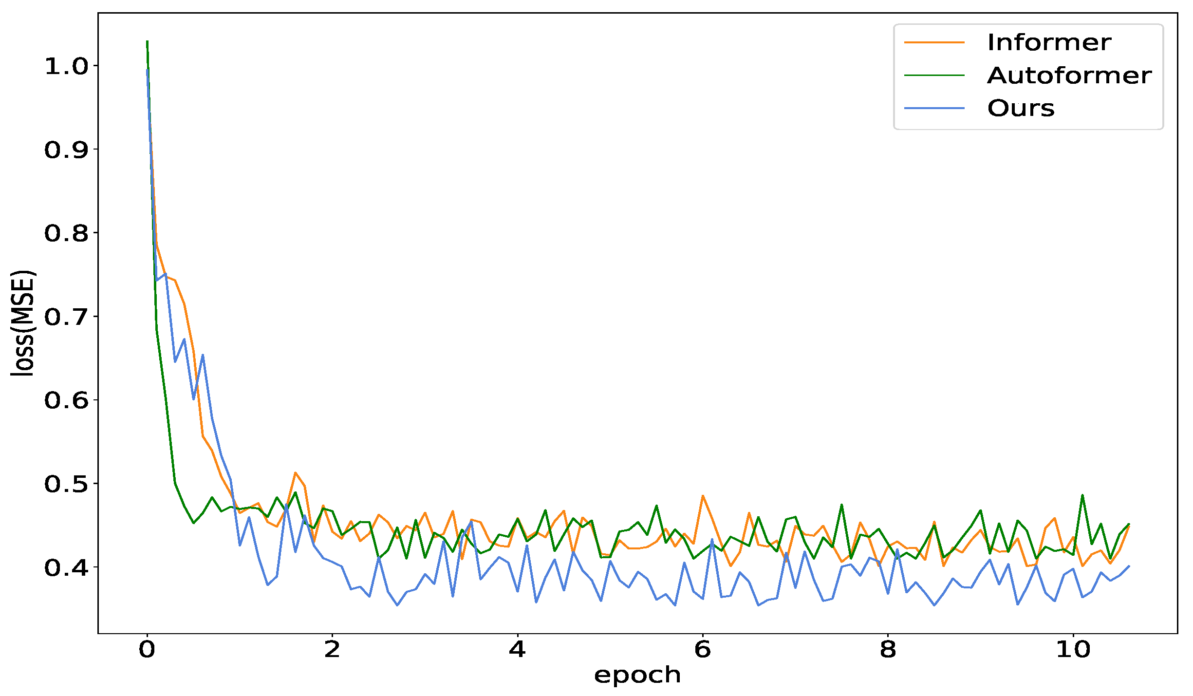
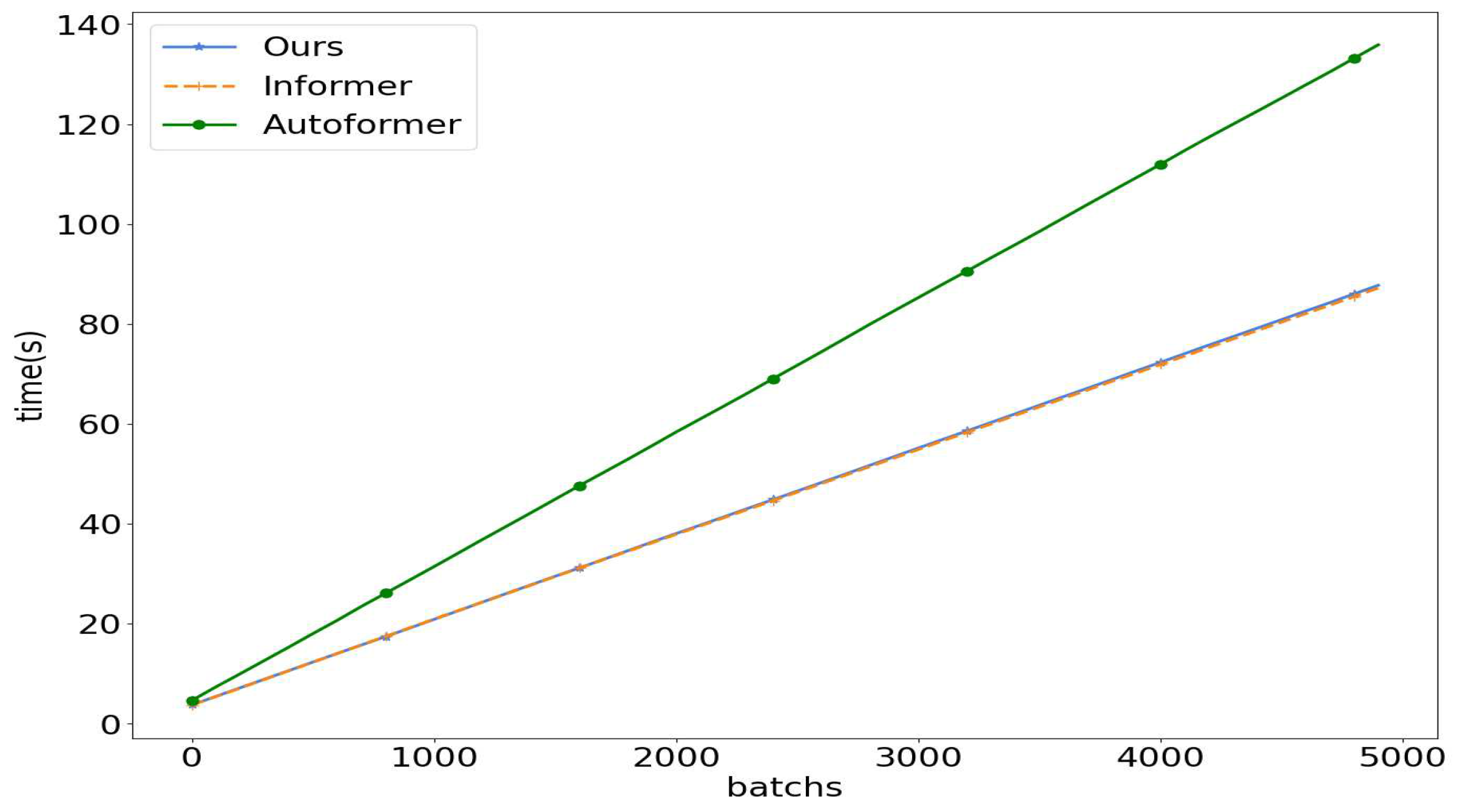
In this experiment, we compare our proposed Informer with the Season-aware Block model with other models to assess its training and inference efficiency. As shown in Figure 5, at the beginning of training, our model’s loss decrease slightly slower. However, as the number of epochs increased, it ultimately achieves a lower error rate compared to other models. It is worth noting that the losses of all three models decreased rapidly in the early stages, mainly due to the simplicity of the ElecZJ dataset. In Figure 6, we compare the inference time of Informer, Autoformer, and our model. We find that adding the Season-aware Block does not significantly increase the inference time, which is almost the same as that of the Informer and much lower than that of the complex-structured Autoformer.

5.6. Ablation studies

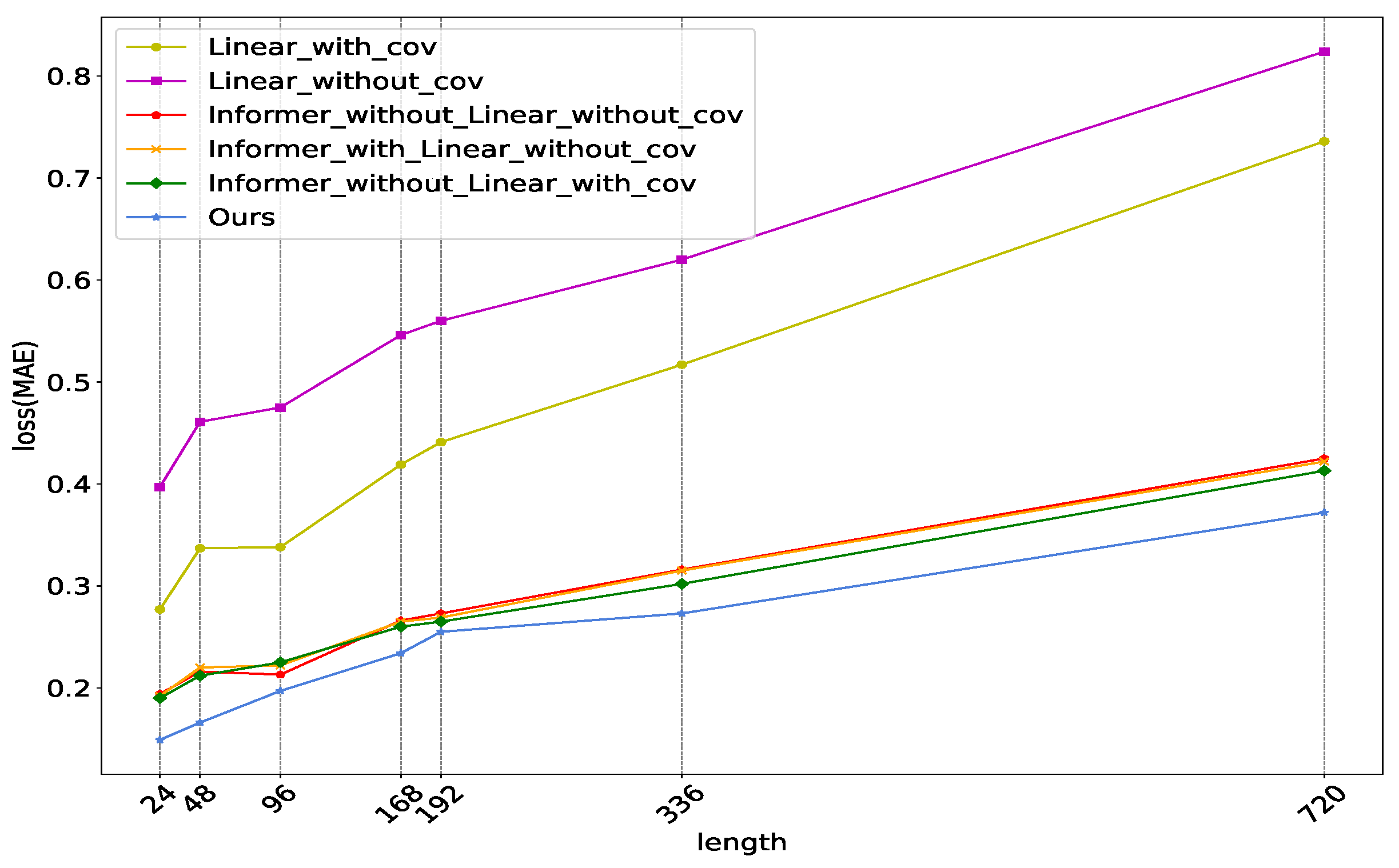
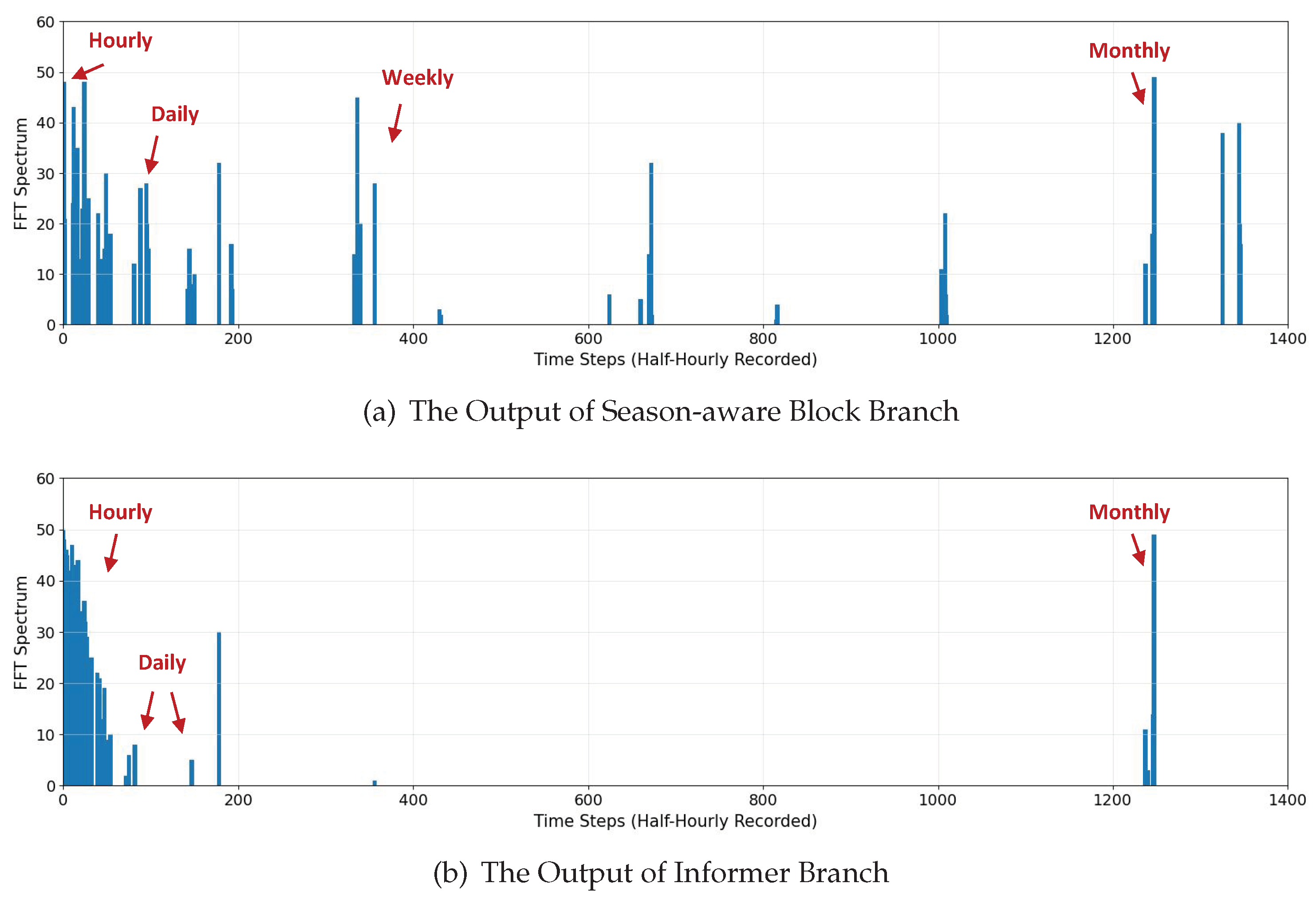
According to Figure 7, we can observe that the Linear model with artificial covariates outperforms the Linear model without covariates. Furthermore, "Ours" also significantly outperforms the "Informer with Linear without cov" combination. This is consistent with the observation in Figure 8b that the Season-aware Block’s output cycle is more similar to the human social cycle. This suggests that the Season-aware branch is more sensitive to artificial covariates and can better learn the human social cycle information. "Informer without Linear without cov" is only slightly lower than "Informer without Linear with cov". This indicates that the Informer model mainly learns information from the LookBack

V_{1 : n}

in the input data and is relatively insensitive to the artificial prior period information in the covariates. "Ours", which refers to "Informer with linear with cov", significantly outperforms "Linear with cov" and "Informer without linear with cov", indicating that by combining the two branches, we can better leverage the complex period information in LookBack and the social cycle prior information in the artificial covariates to achieve better predictive performance.

5.7. Model Analysis

According to Figure 8, it can be observed that the Informer branch, which is based on ProbSparse self-attention, tends to learn high-frequency information and excels in extracting periodic information within 48 time steps. Conversely, the Season-aware Block, which is based on linear layers, is more sensitive to artificial covariates and low-frequency information. This makes it more effective in mining information related to human social cycles, such as hourly, daily, weekly, monthly, and so on.

6. Conclusions

This paper proposes a deep learning model for LSTF tasks that achieves state-of-the-art performance on multiple tasks, including a significant lead in electricity prediction, without increasing training and inference costs compared to Informer. Our model introduces a Season-aware Block based on linear layers on top of Informer, enhancing the model’s sensitivity to artificial temporal covariates. Thsi allows the model to better handle sudden changes in power consumption due to holidays. We also demonstrate the effectiveness of this structure through ablation and comparison experiments. Finally, extensive experiments show that our model achieves the best prediction performance on seven benchmark datasets compared to five advanced algorithms.

Author Contributions

Conceptualization, Y.C. and P.Z.; methodology, Y.C. and Z.L.; writting—original draft preparation, Y.C. and Z.L.; writing—review and editing, P.Z. All authors have read and agreed to the published version of the manuscript.

Funding

This research received no external funding.

Institutional Review Board Statement

Not applicable.

Informed Consent Statement

Not applicable.

Data Availability Statement

Data are unavailable due to privacy.

Acknowledgments

Not applicable.

Conflicts of Interest

The authors declare no conflict of interest.

Appendix A

Appendix A.1. Fast Fourier Transform

The Fast Fourier Transform (FFT) algorithm is a computationally efficient method for calculating the discrete Fourier transform (DFT) of a given signal. A continuous-time signal

f (t)

with a period T, can be represented as a sum of imaginary exponential terms

e^{j n w t}

, known as the complex form of Fourier series,where

w = \frac{2 π}{T}

is the angular frequency and t is the time steps:

f (t) = \sum_{n = - \infty}^{+ \infty} c_{n} e^{jnwt},

(A1)

c_{n} = \frac{1}{T} \int_{- \frac{T}{2}}^{\frac{T}{2}} f (t) e^{- jnwt} dt,

(A2)

Similarly, the complex form of Fourier series for a discrete periodic sequence is:

f_{N} (k) = \sum_{n = 0}^{N - 1} c_{n} e^{jnwk},

(A3)

c_{n} = \frac{1}{N} \sum_{k = 0}^{N - 1} f_{N} (k) e^{- jnwt},

(A4)

Based on the coefficients

c_{n}

of each imaginary exponential term, the discrete Fourier transform(DFT) of a periodic sequence is defined as:

F_{N} (n) = \sum_{k = 0}^{N - 1} f_{N} (k) e^{- jnwk}, n = 0, 1, . . ., N - 1,

(A5)

The original periodic sequence can be obtained by inverse transformation:

f_{N} (k) = \frac{1}{N} \sum_{n = 0}^{N - 1} F_{N} (n) e^{jnwk},

(A6)

The Fast Fourier Transform (FFT) takes advantage of the symmetry and other properties of imaginary exponential terms to simplify the calculation of Discrete Fourier Transform (DFT), thereby improving the computational speed of computers. The computational result of FFT is completely consistent with that of DFT. Firstly, separate the odd and even terms in the Discrete Fourier Transform(assume

N = 2^{l}

\begin{matrix} \begin{matrix} F_{N} (n) & = \sum_{k = 0}^{N - 1} f_{N} (k) e^{- j n w k} \\ = \sum_{r = 0}^{N / 2 - 1} f_{N} (2 r) e^{- j n w \cdot 2 r} + \sum_{r = 0}^{N / 2 - 1} f_{N} (2 r + 1) e^{- j n w \cdot (2 r + 1)} \\ = \sum_{r = 0}^{N / 2 - 1} f_{N / 2}^{'} (r) e^{- j n \frac{w}{2} \cdot r} + \sum_{r = 0}^{N / 2 - 1} f_{N / 2}^{″} (r) e^{- j n \frac{w}{2} \cdot r} \cdot e^{- j n w}, \end{matrix} \end{matrix}

(A7)

The odd and even terms in the original periodic sequence

f_{N} k

are treated as new sequences

f_{N / 2}^{'}

and

f_{N / 2}^{″}

with a period of N/2, so:

\begin{matrix} F_{N} (n) & = \sum_{r = 0}^{N / 2 - 1} f_{N / 2}^{'} (r) e^{- j n \frac{w}{2} \cdot r} + \sum_{r = 0}^{N / 2 - 1} f_{N / 2}^{″} (r) e^{- j n \frac{w}{2} \cdot r} \cdot e^{- j n w} \\ = F_{\frac{N}{2}}^{'} (n) + e^{- j n w} \cdot F_{\frac{N}{2}}^{″} (n), \end{matrix}

(A8)

At this point, the discrete Fourier transform (DFT) of N data points is converted into two

\frac{N}{2}

data points of discrete Fourier transform, which can be quickly solved based on the symmetry of imaginary exponents, thus reducing the computational load.

References

Zhou, H.; Zhang, S.; Peng, J.; Zhang, S.; Li, J.; Xiong, H.; Zhang, W. Informer: Beyond efficient transformer for long sequence time-series forecasting. Proceedings of the AAAI conference on artificial intelligence, 2021, Vol. 35, pp. 11106–11115.
Torres, J.F.; Hadjout, D.; Sebaa, A.; Martínez-Álvarez, F.; Troncoso, A. Deep learning for time series forecasting: a survey. Big Data 2021, 9, 3–21. [Google Scholar] [CrossRef] [PubMed]
Wu, H.; Xu, J.; Wang, J.; Long, M. Autoformer: Decomposition transformers with auto-correlation for long-term series forecasting. Advances in Neural Information Processing Systems 2021, 34, 22419–22430. [Google Scholar]
Vaswani, A.; Shazeer, N.; Parmar, N.; Uszkoreit, J.; Jones, L.; Gomez, A.N.; Kaiser, Ł.; Polosukhin, I. Attention is all you need. Advances in neural information processing systems 2017, 30. [Google Scholar]
Kitaev, N.; Kaiser, Ł.; Levskaya, A. Reformer: The efficient transformer. arXiv preprint arXiv:2001.04451 2020.
Zeng, A.; Chen, M.; Zhang, L.; Xu, Q. Are transformers effective for time series forecasting? Proceedings of the AAAI conference on artificial intelligence, 2023, Vol. 37, pp. 11121–11128.
Dosovitskiy, A.; Beyer, L.; Kolesnikov, A.; Weissenborn, D.; Zhai, X.; Unterthiner, T.; Dehghani, M.; Minderer, M.; Heigold, G.; Gelly, S.; others. An image is worth 16x16 words: Transformers for image recognition at scale. arXiv preprint arXiv:2010.11929 2020.
Salinas, D.; Flunkert, V.; Gasthaus, J.; Januschowski, T. DeepAR: Probabilistic forecasting with autoregressive recurrent networks. International Journal of Forecasting 2020, 36, 1181–1191. [Google Scholar] [CrossRef]
Bai, S.; Kolter, J.Z.; Koltun, V. An empirical evaluation of generic convolutional and recurrent networks for sequence modeling. arXiv preprint arXiv:1803.01271 2018.
Wu, N.; Green, B.; Ben, X.; O’Banion, S. Deep transformer models for time series forecasting: The influenza prevalence case. arXiv preprint arXiv:2001.08317 2020.
Li, S.; Jin, X.; Xuan, Y.; Zhou, X.; Chen, W.; Wang, Y.X.; Yan, X. Enhancing the locality and breaking the memory bottleneck of transformer on time series forecasting. Advances in neural information processing systems 2019, 32. [Google Scholar]
Yu, F.; Koltun, V.; Funkhouser, T. Dilated residual networks. Proceedings of the IEEE conference on computer vision and pattern recognition, 2017, pp. 472–480.
Kingma, D.P.; Ba, J. Adam: A method for stochastic optimization. arXiv preprint arXiv:1412.6980 2014.
He, K.; Zhang, X.; Ren, S.; Sun, J. Deep residual learning for image recognition. Proceedings of the IEEE conference on computer vision and pattern recognition, 2016, pp. 770–778.
Hochreiter, S.; Schmidhuber, J. Long short-term memory. Neural computation 1997, 9, 1735–1780. [Google Scholar] [CrossRef] [PubMed]

Figure 4. The composition of Infomer with Season-aware Block. (a): Season-aware Block consists of Linear, ReLU and Layer Normalization. (b): The Multi-head ProbSparse self-attention Block consists of many parallel ProbSparse Self-Attention structures. (c): The main component of Distilling is the max-pooling operation with a stride of n, which enables a rapid reduction in features size. (d): The Masked Multi-head ProbSparse self-attention serves as the first block in the decoder.

Figure 5. Training curve comparison among the Informer, Our Model, Autoformer in ElecZJ dataset with prediction time steps is 720.

Figure 6. Comparison of computation time curves for the Informer, Our Model, and Autoformer in the ElecZJ dataset, with a prediction time step of 720.

Figure 7. Comparison of two base-branches selection methods (Linear & Informer) with and without covariates. Linear policy refers to a model that only includes the Season-aware Block. Informer policy refers to a model that only includes the Informer branch. Ours refers to the Informer Model with Season-aware Block and input containing covariates. The ’cov’ represents covariates. In all experiments, we fixed the input length to be 96 and varied the predict length to be 24, 48, 96, 168, 192, 336 and 720.

Figure 8. Frequency plot of fast Fourier transform. Through fast Fourier transform, the outputs of our model’s two branches, the Informer branch and the Season-aware Block branch, are mapped from the time domain to the frequency domain to observe the periodic information learned by different branches. (b) shows the fast Fourier transform frequency plot of Season-aware Block branch, (a) displays fast Fourier transform frequency plot of Informer branch.

Disclaimer/Publisher’s Note: The statements, opinions and data contained in all publications are solely those of the individual author(s) and contributor(s) and not of MDPI and/or the editor(s). MDPI and/or the editor(s) disclaim responsibility for any injury to people or property resulting from any ideas, methods, instructions or products referred to in the content.

© 2023 by the authors. Licensee MDPI, Basel, Switzerland. This article is an open access article distributed under the terms and conditions of the Creative Commons Attribution (CC BY) license (http://creativecommons.org/licenses/by/4.0/).

Copyright: This open access article is published under a Creative Commons CC BY 4.0 license, which permit the free download, distribution, and reuse, provided that the author and preprint are cited in any reuse.

MDPI Initiatives

Important Links

Choose an area of interest and we will send you notifications of new preprints at your preferred frequency.

Disclaimer

Informer Model with Season-Aware Block for Efficient Power Series Forecasting

Abstract

1. Introduction

2. Related Work

2.1. Models for LSTF

2.2. temporal covariates

3. Preliminary

4. Informer with Season-aware Block

4.1. Model inputs

4.2. Season-aware Block

4.3. Informer

4.3.1. ProbSparse Self-attention

4.3.2. Encoder

4.3.3. Decoder

4.3.4. Loss Function

5. Results

5.1. Datasets

5.2. Implement details

5.3. BaseLines

5.4. Accuracy

5.5. Train and Inference Speed

5.6. Ablation studies

5.7. Model Analysis

6. Conclusions

Author Contributions

Funding

Institutional Review Board Statement

Informed Consent Statement

Data Availability Statement

Acknowledgments

Conflicts of Interest

Appendix A

Appendix A.1. Fast Fourier Transform

References

MDPI Initiatives

Important Links

Subscribe