ESP Lifted Oil Field: Basic Model for Control, and Comparison of Simulation Tools

Preprint

Article

ESP Lifted Oil Field: Basic Model for Control, and Comparison of Simulation Tools

Altmetrics

Downloads

Views

Comments

A peer-reviewed article of this preprint also exists.

Bernt Lie^*

This version is not peer-reviewed

Submitted:

15 December 2023

Posted:

19 December 2023

You are already at the latest version

Alerts

Abstract

Optimal operation of petroleum production is important in a transition from energy systems based on fossil fuel to sustainable systems. One sub-process in petroleum production deals with transport from the (subsea) well-bore to a topside separator. A simple model in [] of Electric Submersible Pump [ESP] lifted production was previously streamlined into a dynamic model suitable for illustration of the dynamics of oil transport, as well for control studies, with some comparison of two popular modeling languages: Modelica, and ModelingToolkit for Julia, []. Here, the discussion on dimensionless equipment models goes into more detail, and the comparison between Modelica and ModelingToolkit is significantly expanded upon with code comparison, numerical performance, and more experiments. Some added possibilities with ModelingToolkit and Julia wrt. sensitivity analysis and control design is included.

Keywords:

Subject: Engineering - Control and Systems Engineering

1. Introduction

1.1. Background

Petroleum products have been key energy carriers for more than a century. Current focus on climate1 implies a change towards sustainable energy carriers. To succeed in this change, a transition period from the use of fossil fuel is necessary. In the transition, improved operation of petroleum production through model based optimal operation will be necessary. Petroleum production entails slow (reservoir; months) and fast (reservoir-to-separator; seconds) subsystems; this is a focus of on-going research project “DigiWell”2. Vertical transport of petroleum from oil well to surface requires sufficient pressure to counteract gravitational and friction forces. If the oil-well heel pressure is insufficient for such transport, either (i) gas is injected in the vertical pipe to “blow” the petroleum fluids to the surface [“gas lifted”], or (ii) an Electric Submersible Pump [ESP] is installed in the vertical pipe to increase the pressure [“ESP lifted”] sufficiently. Here, the focus is on the dynamics of transport from the reservoir formation to a surface manifold via an ESP, and further horizontal transport from the manifold to a separator.

Industrial simulation tools typically put main emphasis on the dynamics of the reservoir (time constant: months) and use steady state models for the reservoir-to-surface transport. This emphasis is inadequate for daily operation and control. Here, a simplified, yet complete, dynamic model for oil transport from reservoir to separator is discussed. The model provides an understanding of the dynamic behavior of such systems, and is suitable for industrial control design, as well as for control and petroleum production studies. Emphasis is put on a simple, yet stringent model development, while avoiding variable unit complexities.

1.2. Previous work

Sharma and Glemmestad [1] (see also Sharma [3]) provide a dynamic model of oil transport from reservoir to separator suitable for control design. Binder et al. [4] discuss an older model; other models typically are CFD models, which are too complex for control design.

Sharma’s model considers a case with 4 vertical pipes from oil reservoirs to a single manifold, with 2 horizontal pipes from the manifold to a single separator. Each vertical pipe has an ESP and a choke valve at a common manifold entrance; the pump speeds can be manipulated individually. The horizontal pipes have booster pumps to counteract friction effects. The original ESP model includes induction motors, but the dynamics of the pump actuator is fast, and is neglected in later work. Sharma and Glemmestad [1] provide a novel ESP model, a simple model for a booster pump, and use a valve model based on on the ANSI/ISA S75.01 standard3. The model in Sharma and Glemmestad [1] was re-structured and simplified in Lie [2], emphasizing dimensionless equipment models, and thereby eliminating some level of complexity in common industry models.

The model with ESP in Sharma and Glemmestad [1] is mainly relevant for the production of heavy oil. Several papers use this model in advanced industrial control studies, Krishnamoorthy et al. [5], Delou et al. [6], Santana et al. [7].

Mixtures of liquid oil and water form an emulsion when stirred (e.g., in a multi-stage ESP); for such emulsions, the viscosity — and hence the friction — varies dramatically with water content, Justiniano and Romero [8]. Sharma and Glemmestad [1] assume an unrealistic linear viscosity dependence on water fraction.

1.3. Structure of paper

Section 2 gives an overview of the transport system from oil reservoir via manifold to a separator, and key equipment models. Section 3 develops a simple mechanistic model of the system. Section 4 contrasts two modeling languages for simulation: Modelica and Julia’s ModelingToolkit. Section 5 illustrates model behavior and the use of modeling/simulation tools for analysis and control. Finally, Section 6 provides some conclusions.

2. System description

Production of a mixture of water and crude oil in liquid phase is considered, where evaporation of liquids is assumed negligible.

2.1. System topology

Oil production systems merge several boreholes from the same or different reservoirs through vertical pipes into a manifold. Normally, more than one horizontal transport pipe is needed from the manifold to a separator for sufficient transport capacity. Water is commonly injected into the manifold to reduce friction loss in the horizontal pipes; the added water is typically recycled from the separator, and is at close to production temperature. 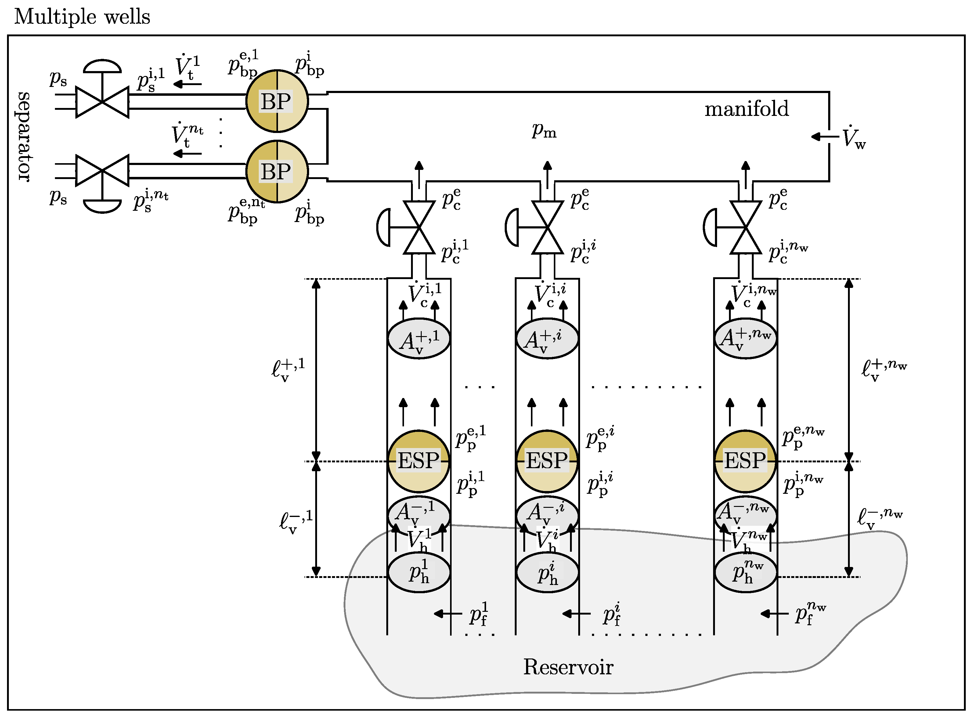Figure 1 shows a system with

n_{w}

wells/vertical pipes via a common manifold to

n_{t}

transportation/horizontal pipes leading to the separator.

In Figure Figure 1 ,

p_{f}^{j}

is formation pressure for well j,

p_{h}^{j}

is bore-hole heel pressure,

{\dot{V}}_{h}^{j}

is volumetric heel flow rate,

A_{v}^{-, j}

is vertical cross sectional area below the ESP pump,

ℓ_{v}^{-, j}

is the length of the vertical pipe below the ESP pump,

p_{p}^{i, j}

is inlet pressure to the (ESP) pump,

p_{p}^{e, j}

is effluent pressure after the (ESP) pump,

A_{v}^{+, j}

is vertical cross sectional area above the ESP pump,

ℓ_{v}^{+, j}

is the length of the vertical pipe above the ESP pump,

{\dot{V}}_{c}^{i, j}

is volumetric flow rate at the inlet to the choke valve,

p_{c}^{i, j}

is pressure at the inlet to the choke valve,

p_{c}^{e, j}

is pressure at the effluent from the choke valve. Next,

p_{m}

is manifold pressure, while

{\dot{V}}_{w}

is water added to the manifold to reduce viscosity. At the outlet from the manifold,

p_{bp}^{i, j}

is the influent pressure to the booster pump (BP),

p_{bp}^{e, j}

is effluent pressure after the booster pump,

{\dot{V}}_{t}^{j}

is volumetric flow rate in a transport pipe from manifold to separator,

p_{s}^{i, j}

is pressure at the inlet to the valve into the separator, and

p_{s}^{e, j} = p_{s}

is the separator pressure.

For simplicity, it is assumed that

A_{v}^{-, j} = A_{v}^{+, j} = A_{v}

. All vertical pipes are assumed connected to the same manifold pressure

p_{m}

; hence effluent choke pressure satisfies

p_{c}^{e, j} = p_{c}^{e} = p_{m}

for all j. The influent pressure to the booster pumps,

p_{bp}^{i, j}

are all assumed to be equal to the outlet pressure from the manifold, and have the same value,

p_{bp}^{i, j} = p_{bp}^{i} = p_{m}

. Likewise, all transport pipes end up in the same separator:

p_{s}^{e, j} = p_{s}

for all j.

2.2. Fluid properties

The petroleum fluid properties are important. Density

ρ

varies with pressure p and temperature T,

ρ (p, T)

. Neglecting temperature dependence, and assuming constant isothermal compressibility

β_{T}

ρ (p)

is given as

ρ = ρ_{0} exp (β_{T} (p - p_{0}))

(1)

where

(ρ_{0}, p_{0})

is some reference state.

Defining water cut

χ_{w}

χ_{w} ≜ {\dot{V}}_{w} / \dot{V}

: volumetric flow rate of water divided by total flow rate of the fluid, total density

ρ

can be expressed as

ρ = χ_{w} ρ_{w} + (1 - χ_{w}) ρ_{o};

(2)

here,

ρ_{w}

and

ρ_{o}

are constant densities of pure water and crude oil, respectively.

In reality, water and crude oil have different isothermal compressibilities. Here, we simplify and assume an overall value for

β_{T}

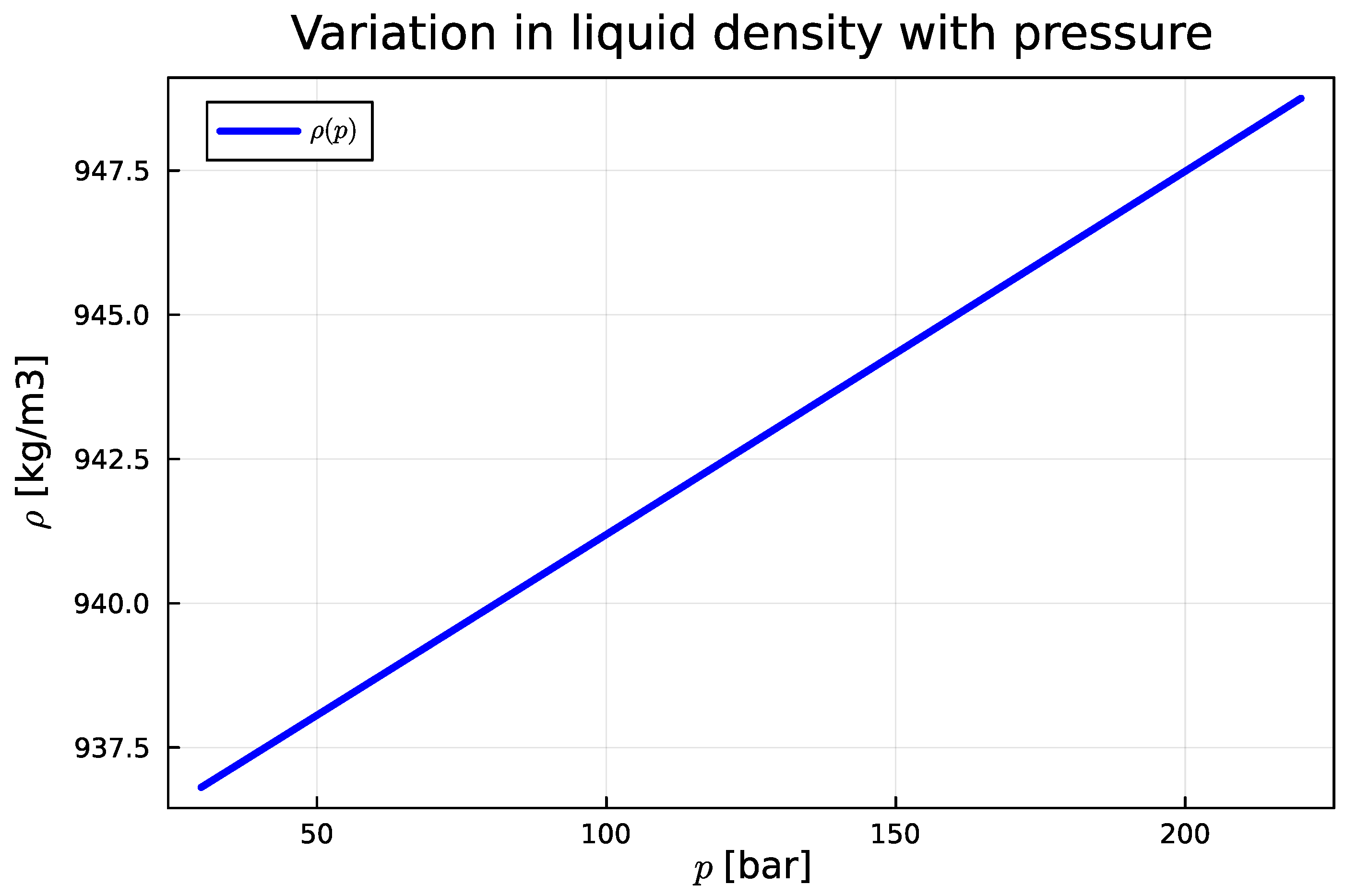
. Using data in Appendix A1, density

ρ

varies ca.

10 kg / m^{3}

with pressure variation in the range 25–

225 bar

, Figure 2.

We thus assume constant density in pipes, but a pressure-dependent density will be assumed in the manifold.

Sharma and Glemmestad [1] propose a simple linear mixing rule for kinematicviscosity

ν

ν = χ_{w} ν_{w} + (1 - χ_{w}) ν_{o} .

(3)

With

ν

known, dynamic viscosity

μ

can be computed (if needed) as

μ = ν ρ .

The linear interpolation model of Eq. 3 is used here to ease comparison with results in Sharma and Glemmestad [1], even though it is not physically realistic [8].

2.3. Well-bore production

Total production from the reservoir (formation pressure

p_{f}

) relates volumetric petroleum fluid rate

{\dot{V}}_{h}

at the well-bore heel as

{\dot{V}}_{h} \propto p_{f} - p_{h}

, where

p_{h}

is heel pressure and the proportionality constant

C_{pi}

is the productivity index,

{\dot{V}}_{h} = C_{pi} \cdot (p_{f} - p_{h});

C_{pi}

is unit-dependent. Here, we instead propose a dimensionless form,

{\dot{V}}_{h} = {\dot{V}}_{pi}^{c} \frac{p_{f} - p_{h}}{p_{pi}^{ς}}

(4)

where

{\dot{V}}_{pi}^{c}

is the productivity index capacity in the same unit as

{\dot{V}}_{h}

, and

p_{pi}^{ς}

is scaling pressure with the same unit as

p_{f}, p_{h}

2.4. Pump models

Electric Submersible Pump

Pump models are often given as

Δ p_{p} = ρ g h_{p};

(5)

here,

h_{p} = h_{p} (\dot{V}, f_{p})

is pump head with volumetric flow rate

\dot{V}

and control input

f_{p}

— rotational pump frequency

Hz

Sharma and Glemmestad [1] provide values for minimal, maximal, and best-efficiency-point flow rates,

\begin{matrix} \frac{{\dot{V}}_{min}}{{\dot{V}}_{min, 0}} & = \frac{f_{p}}{f_{p, 0}} \end{matrix}

(6)

\begin{matrix} \frac{{\dot{V}}_{max}}{{\dot{V}}_{max, 0}} & = \frac{f_{p}}{f_{p, 0}} \end{matrix}

(7)

\begin{matrix} \frac{{\dot{V}}_{η}}{{\dot{V}}_{η, 0}} & = \frac{f_{p}}{f_{p, 0}} . \end{matrix}

(8)

In Sharma and Glemmestad [1], a comprehensive model for the pump head of a multi-stage ESP is developed. To ease change of units, their model is here rewritten in dimensionless form

\begin{matrix} \frac{h_{p} (\dot{V}, f_{p})}{h_{p, 0}} & = {(\frac{f_{p}}{f_{p, 0}})}^{2} + \sum_{j = 1}^{3} a_{j} {(\frac{f_{p}}{f_{p, 0}})}^{2 - j} {(\frac{\dot{V}}{{\dot{V}}^{ς}})}^{j} . \end{matrix}

(9)

In Eq. 9,

h_{p, 0}

is a nominal scaling head,

f_{p}

is the pump rotational frequency in the same unit as that of the nominal rotational frequency

f_{p, 0}

\dot{V}

is the actual volumetric flow rate out of the pump,

{\dot{V}}^{ς}

a scaling flow rate, and

a_{1}, \dots, a_{3}

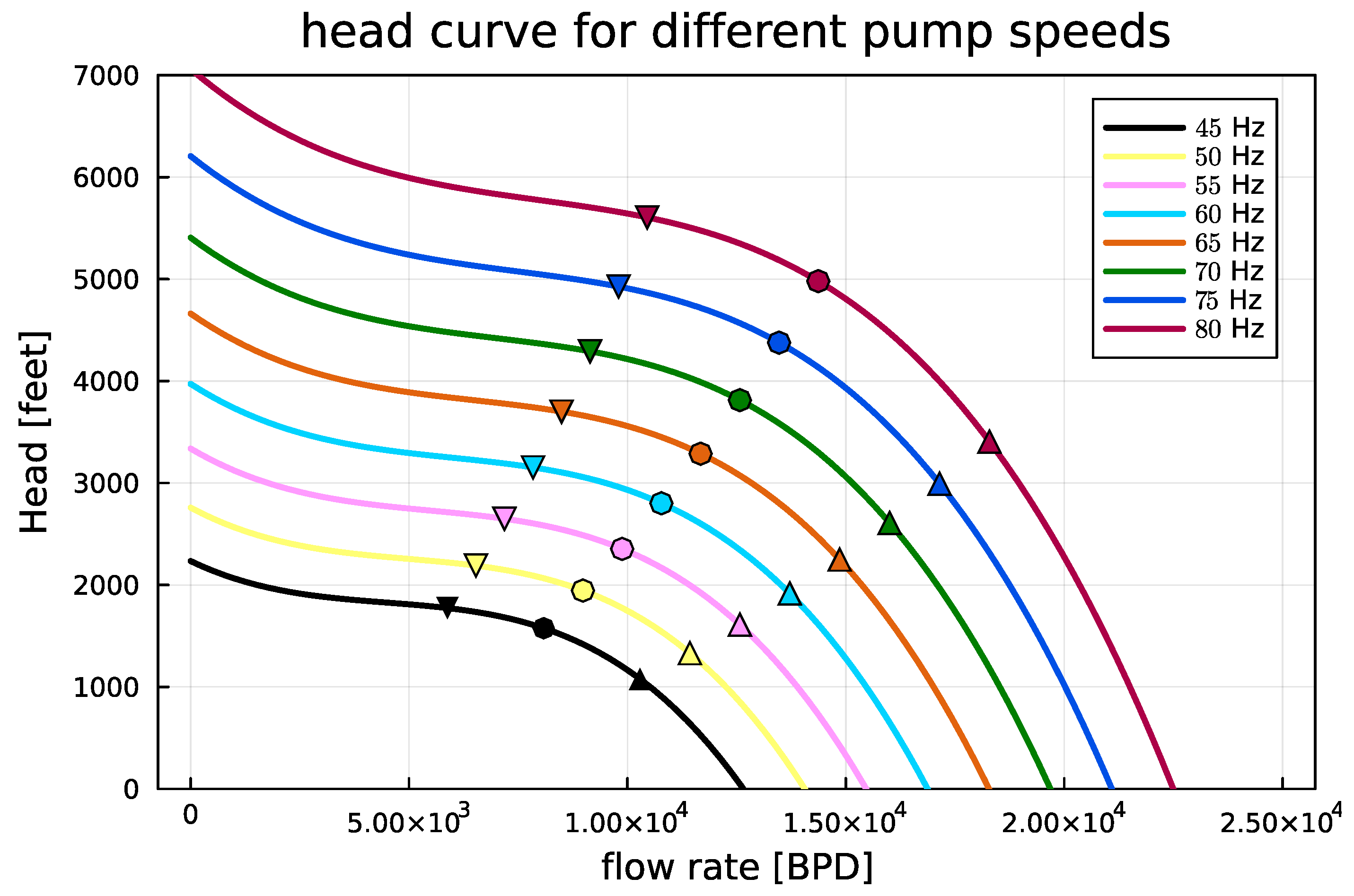
are dimensionless model parameters5. Sharma and Glemmestad [1] include a head curve plot; the result in Figure 3 based on a dimensionless model is identical to their plot.

In addition, Sharma and Glemmestad [1] provide a model for the mechanical power requirement

{\dot{W}}_{p}^{m} = {\dot{W}}_{p}^{m} (\dot{V}, f_{p})

for operating the pump6, again rewritten in dimensionless form,

\begin{matrix} \frac{{\dot{W}}_{p}^{m}}{{\dot{W}}_{p, 0}^{m}} & = {(\frac{f_{p}}{f_{p, 0}})}^{3} + \sum_{j = 1}^{4} b_{j} {(\frac{f_{p}}{f_{p, 0}})}^{3 - j} {(\frac{\dot{V}}{{\dot{V}}^{ς}})}^{j} . \end{matrix}

(10)

In Eq. 10,

{\dot{W}}_{p, 0}^{m}

is a nominal scaling power consumption to operate the pump,

b_{1}, \dots, b_{4}

are dimensionless model parameters, while

f_{p}

and

\dot{V}

are as above.

The actual power added to the fluid is

{\dot{W}}_{p} = Δ p_{p} \dot{V},

(11)

which gives the efficiency as

η = \frac{{\dot{W}}_{p}}{{\dot{W}}_{p}^{m}} = \frac{Δ p_{p} \dot{V}}{{\dot{W}}_{p}^{m}}

(12)

where it is assumed that

{\dot{W}}_{p}

and

{\dot{W}}_{p}^{m}

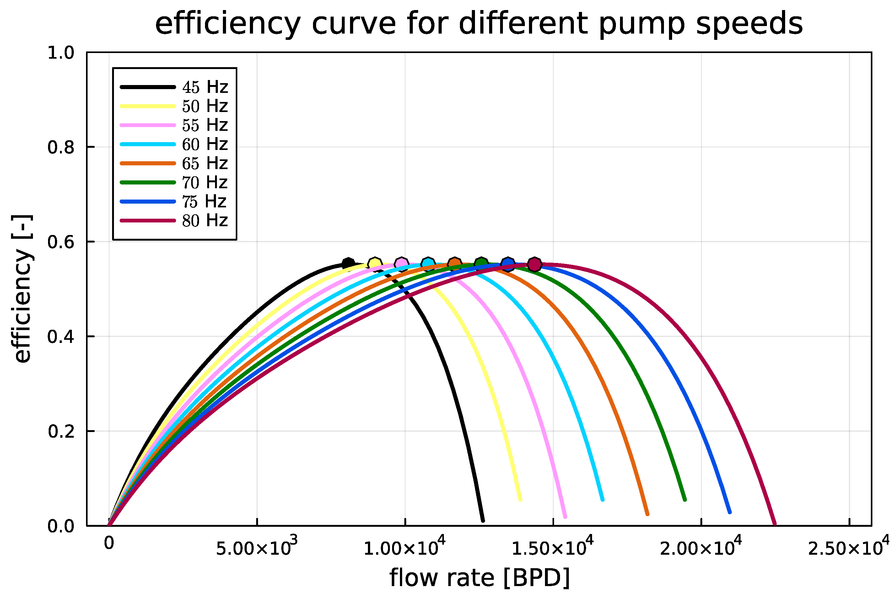
have the same units. Sharma and Glemmestad [1] include an efficiency curve plot; the result in Figure 4 based on a dimensionless model is identical to their plot.

Booster pump

For the booster pump in horizontal pipes, a simpler model is suggested in Sharma and Glemmestad [1], rewritten in dimensionless form as

\frac{Δ p_{bp} (f_{bp})}{Δ p_{bp, 0}} = {(\frac{f_{bp}}{f_{bp, 0}})}^{2}

(13)

Here,

Δ p_{bp} (f_{bp})

is the pressure increase at the given pump frequency/speed

f_{bp}

, in the same unit as

Δ p_{bp, 0}

— which is the pressure increase at the nominal pump frequency

f_{bp, 0}

Pump control input

In reality, the pump speed (

f_{p}

f_{bp}

) is not a control input. Instead, a motor is used to control the torque applied to the aggregate of motor and pump.

In Sharma [3], a model of the induction motor driving the ESP is developed. The experience [3] is that the motor dynamics is much faster than that of the mechanical system; hence in most of his work, Sharma [3] neglects the motor dynamics. However, it is not clear whether Sharma [3] considers the mechanical dynamics of accelerating the pump itself. This dynamics would be described by the kinetic energy balance in rotational form (the “swing equation”), which can be written as

\frac{d K}{d t} = P_{i} - {\dot{W}}_{p}^{m}

with kinetic energy K

K = \frac{1}{2} J_{t} ω_{p}^{2},

J_{t}

is the total moment of inertia for the pump, the motor, and a possible flywheel, while

P_{i}

is the input power from the motor (control input), and

{\dot{W}}_{p}^{m}

is as in Eq. 10.

In Sharma [3], the moment of inertia is approximately given as

J \approx 71 kg m^{2}

. It is not clear whether this is the motor moment of inertia or the total moment of inertia. However, using such a moment of inertia leads to a pump time constant which is still much faster than the dynamics of the flow

{\dot{V}}_{v}

, etc., hence the pump/motor dynamics is neglected here, and for simplicity, it is assumed that

f_{p}

is a control input.

2.5. Valve models

Sharma and Glemmestad [1] base their valve models on the ANSI/ISA S75.01 standard7. Here, instead a dimensionless description is proposed with extension to a control input,

\dot{m} = {\dot{m}}_{v}^{c} \cdot f (u_{v}) \frac{ρ_{i}}{ρ_{e}} \sqrt{\frac{(p_{i} - p_{e}) / p^{ς}}{ρ_{i} / ρ^{ς}}}

(14)

where

{\dot{m}}_{v}^{c}

is the valve mass flow rate capacity,

u_{v} \in [0, 1]

is the valve control signal,

f : [0, 1] \to [0, 1]

is the valve characteristics,

ρ_{i}, ρ_{e}

are influent and effluent densities, respectively,

p_{i}, p_{e}

are influent and effluent pressures, respectively, while

ρ^{ς}, p^{ς}

are scaling density and pressure, respectively.

2.6. Friction loss

The friction drop along the pipe can be given by the Darcy-Weisbach model8 as

\frac{Δ p_{f}}{ℓ} = f_{D} \frac{ρ}{2} \frac{v^{2}}{D}

(15)

where

f_{D}

is Darcy’s friction factor given by Colebrook’s9 implicit expression. One explicit approximation to Colebrook’s expression is due to Swamee and Jain [9],

\frac{1}{\sqrt{f_{D}}} = - 2 \cdot {log}_{10} (\frac{5.74}{N_{Re}^{0.9}} + \frac{ϵ / D}{3.7}),

(16)

where

N_{Re}

is the Reynolds number,

N_{Re} = \frac{ρ v D}{μ} = \frac{v D}{ν},

(17)

μ

is dynamic viscosity,

ν

is kinematicviscosity, and

ϵ

is the “roughness height” of the pipe internal surface. Linear velocity v is related to volumetric flow rate

\dot{V}

\dot{V} = v A

(18)

where A is the cross-sectional area of the pipe.

2.7. Why dimensionless models?

Example: ESP pump model

As a first example, consider the ESP model in Eq. 9. In the original formulation in Sharma and Glemmestad [1],10

h_{p} = {\bar{a}}_{0} \frac{f_{p}}{f_{p, 0}} + {\bar{a}}_{1} \frac{f_{p}}{f_{p, 0}} \dot{V} + {\bar{a}}_{2} {\dot{V}}^{2} + {\bar{a}}_{3} \frac{f_{p, 0}}{f_{p}} {\dot{V}}^{3},

(19)

where parameters

{\bar{a}}_{j}

have rather complicated units and the equation is hard-coded to assume11

[\dot{V}] = gal / \min

, while

[h_{p}] = ft

. In practice, either the rest of the model has to be posed using these units, or one has to operate with several copies of variables, e.g.,

{\dot{V}}_{g / m}

and

\dot{V}

, and remember to correctly convert between these versions of the flow rate. Both of these approaches are error-prone, and also require several versions of variables.

A much better solution is to write the model in dimensionless form. The simplest way to do this for the model in Eq. 19, is as

\begin{matrix} \frac{h_{p}}{h_{p, 0}} & = {\tilde{a}}_{0} \frac{f_{p}}{f_{p, 0}} + {\tilde{a}}_{1} \frac{f_{p}}{f_{p, 0}} \frac{\dot{V}}{{\dot{V}}^{ς}} + {\tilde{a}}_{2} {(\frac{\dot{V}}{{\dot{V}}^{ς}})}^{2} + {\tilde{a}}_{3} \frac{f_{p, 0}}{f_{p}} {(\frac{\dot{V}}{{\dot{V}}^{ς}})}^{3} . \end{matrix}

(20)

If we choose

h_{p, 0} \equiv 1 ft

and

{\dot{V}}^{ς} \equiv 1 gal / \min

, then

{\tilde{a}}_{j} \equiv {\bar{a}}_{j}

. Suppose we want to generate the plot in Figure 3. Because that figure plots

h_{p}

ft

(the “native” unit), while the flow rate

\dot{V}

is given in

bbl / d

(“native” unit is

gal / \min

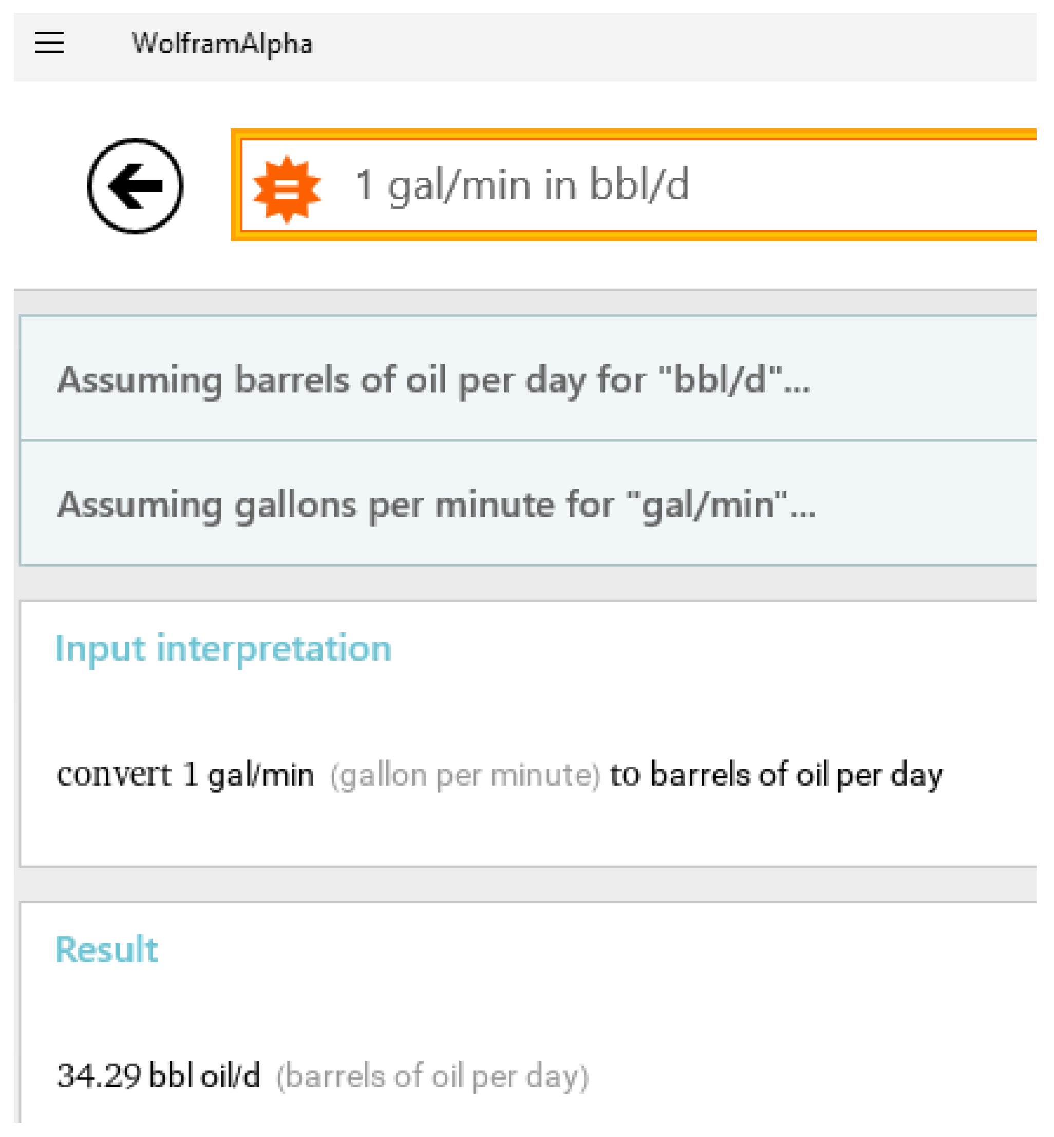
), this result is produced by choosing

{\dot{V}}^{ς} = 1 gal / \min = 34.29 bbl l / d

, which can easily be found using the WolframAlpha app12, Figure 5.

In practice, it may be better to choose a more natural scaling unit, e.g., SI units. In that case, it is necessary to change parameters

{\bar{a}}_{j}

; for the parameters in Eq. 9, the scaling parameters are in SI units, where

{\bar{a}}_{j} \to a_{j}

and

a_{j}

is given in Table A2. To find

a_{j}

, choose

h_{p, 0} = 1 ft = 0.3048 m

{\dot{V}}^{ς} = 1 gal / \min = 6.309 \cdot 10^{- 5} m^{3} / s

, and write Eq. 20 as

\begin{matrix} \frac{h_{p}}{\underset{\to h_{p, 0}}{\underset{︸}{h_{p, 0} {\tilde{a}}_{0}}}} & = \frac{f_{p}}{f_{p, 0}} + \underset{a_{1}}{\underset{︸}{\frac{{\tilde{a}}_{1}}{{\tilde{a}}_{0} {\dot{V}}^{ς}}}} \frac{f_{p}}{f_{p, 0}} \dot{V} + \underset{a_{2}}{\underset{︸}{\frac{{\tilde{a}}_{2}}{{\tilde{a}}_{0} {({\dot{V}}^{ς})}^{2}}}} {\dot{V}}^{2} + \underset{a_{3}}{\underset{︸}{\frac{{\tilde{a}}_{3}}{{\tilde{a}}_{0} {({\dot{V}}^{ς})}^{3}}}} \frac{f_{p, 0}}{f_{p}} {\dot{V}}^{3}, \end{matrix}

where the new

h_{p, 0}

is given in unit

m

a_{1}

a_{2}

a_{3}

are the new, dimensionless parameters in Eq. 9, while new scaling flow rate

\to {\dot{V}}^{ς} = 1 m^{3} / s

. With this modified correlation (

a_{1}, \dots, a_{3}

) for

h_{p}

using SI units, the dimensionless form is as in Eq. 9.

Example: control valve

The ANSI/ISA S75.01 standard13 for compressible (i.e.,

{\dot{m}}_{i} = {\dot{m}}_{e} = \dot{m}

ρ_{i} \neq ρ_{e}

), non-choked fluids without fitting is

C = \frac{\dot{m}}{N_{6} \frac{ρ_{i}}{ρ_{e}} \sqrt{\frac{p_{i} - p_{e}}{ρ_{i}}}} .

(21)

Here, C is the valve coefficient,

\dot{m}

is the mass flow rate through the valve,

ρ_{i}

is the influent density,

ρ_{e}

is the effluent density,

p_{i}

is the influent pressure,

p_{e}

is the effluent pressure,

N_{6}

is used to handle unit conversion. Typically, tabular values for

N_{6}

are given which are valid for different combinations of units for

\dot{m}

ρ

, and p. This makes change of units rather complicated. A dimensionless formulation as in Eq. 14 greatly simplifies the use of the valve model in different units, and also includes a control valve characteristic.

3. Dynamic model

3.1. Balance laws

The model is based on the total mass balance (manifold) and the linear momentum balance (pipes). The total mass balance is expressed as

\frac{d m}{d t} = {\dot{m}}_{i} - {\dot{m}}_{e}

(22)

where m is accumulated mass in the system, t is time,

\dot{m}

is mass flow rate, and indices

(i, e)

denote influent and effluent, respectively.

The linear momentum balance is

\frac{d m}{d t} = {\dot{m}}_{i} - {\dot{m}}_{e} + F,

(23)

where

m

is linear momentum given as

m = m v

with linear velocity v,

\dot{m}

is momentum flow rate given as

\dot{m} = \dot{m} v

, and F is total force. With constant fluid density,

{\dot{m}}_{i} = {\dot{m}}_{e}

, and the momentum balance reduces to Newton’s law,

\frac{d m}{d t} = F

3.2. Vertical pipes with ESP

We assume constant density in the pipes, causing volumetric vertical flow rate

{\dot{V}}_{v}

to be the same everywhere:

{\dot{V}}_{h} = {\dot{V}}_{c}^{i} = {\dot{V}}_{v}

. Furthermore, Eq. 23 reduces to Newton’s law. Momentum is given as

m = \dot{m} v

with

\dot{m} = ρ {\dot{V}}_{v}

, and v related to

{\dot{V}}_{v}

by Eq. 18. The total force is

F = F_{p} + F_{b} - F_{f} - F_{g}

, with

Pressure forces at inlet and outlet of the pipe,

$F_{p} = p_{h} A - p_{c}^{i} A$

(24)
Possible pressure boost due to a pump,

$F_{b} = Δ p_{p} A,$

(25)

with $Δ p_{p}$ given by Eqs. 5, 9,
Friction loss,

$F_{f} = Δ p_{f} A,$

(26)

with $Δ p_{f}$ given by Eqs. 15, 16, 17, 18,
Flow against gravity, with a vertical height h,

$F_{g} = Δ p_{g} A,$

(27)

with

$Δ p_{g} = ρ_{v} g h .$

(28)

In addition, we need information about how flow rate

{\dot{V}}_{v}

relates to the bottom hole pressure via the productivity index, Eq. 4, and how the flow rate

{\dot{V}}_{v}

relates to the choke valve flow, Eq. 14.

The most structured formulation would be to pose the momentum balance (here: Newton’s law) as the differential equation, and add all necessary algebraic equations. However, the OpenModelica DAE solver struggles with such a formulation: the valve equation Eq. 14 is implicit in pressure difference; in the iteration to find

Δ p_{v} = p_{i} - p_{e}

, if

Δ p_{v}

becomes negative, the square root gives a complex number, and the simulation crashes.14 Instead, the differential variable has been changed to

{\dot{V}}_{v}

; then the valve equation can be inverted and expressed as

Δ p_{v} \propto {\dot{V}}_{v}^{2}

The following formulation is used in OpenModelica and ModelingToolkit:

\frac{d {\dot{V}}_{v}}{d t} = \frac{p_{h} - p_{i}^{c} + Δ p_{p} - Δ p_{f} - Δ p_{g}}{ρ_{v} ℓ / A}

(29)

\begin{matrix} ρ_{β}^{0} & = χ_{w} ρ_{w} + (1 - χ_{w}) ρ_{o} \end{matrix}

(30)

\begin{matrix} ν & = χ_{w} ν_{w} + (1 - χ_{w}) ν_{o} \end{matrix}

(31)

\begin{matrix} μ & = ρ_{β}^{0} ν \end{matrix}

(32)

\begin{matrix} ρ_{v} & = ρ_{β}^{0} exp (β_{T} (p_{c}^{i} - p_{β}^{0})) \end{matrix}

(33)

p_{h} = p_{f} - p_{pi}^{ς} \frac{{\dot{V}}_{v}}{{\dot{V}}_{pi}^{c}}

(34)

{\dot{m}}_{v} = ρ_{v} {\dot{V}}_{v}

(35)

p_{i}^{c} = p_{m} + p_{v}^{ς} \frac{ρ_{v}}{ρ_{v}^{ς}} {(\frac{{\dot{m}}_{v}}{{\dot{m}}_{v}^{c}})}^{2} \frac{1}{f_{c}^{2} (u_{v})}

(36)

\begin{matrix} h_{p} & = h_{p, 0} ({(\frac{f_{p}}{f_{p, 0}})}^{2} + a_{1} \frac{f_{p}}{f_{p, 0}} \frac{{\dot{V}}_{v}}{{\dot{V}}^{ς}} \\ + a_{2} {(\frac{{\dot{V}}_{v}}{{\dot{V}}^{ς}})}^{2} + a_{3} \frac{f_{p, 0}}{f_{p}} {(\frac{{\dot{V}}_{v}}{{\dot{V}}^{ς}})}^{3}) \end{matrix}

(37)

\begin{matrix} Δ p_{p} & = ρ_{v} g h_{p} \end{matrix}

(38)

\begin{matrix} v_{v} & = \frac{{\dot{V}}_{v}}{A} \end{matrix}

(39)

\begin{matrix} N_{Re} & = \frac{v_{v} d_{v}}{ν_{v}} \end{matrix}

(40)

\begin{matrix} f_{D}^{v} & = \frac{1}{4 {({log}_{10} (\frac{5.74}{N_{Re}^{0.9}} + \frac{ϵ_{v} / d_{v}}{3.7}))}^{2}} \end{matrix}

(41)

\begin{matrix} Δ p_{f} & = ℓ \cdot f_{D}^{v} \frac{ρ_{v}}{2} \frac{v_{v}^{2}}{d_{v}} \end{matrix}

(42)

\begin{matrix} Δ p_{g} & = ρ_{v} g h . \end{matrix}

(43)

If we only consider the model of a single vertical pipe, we need to specify (i) initial state (e.g.,

{\dot{V}}_{v}

), (ii) all “input” variables, i.e.,

p_{f}

f_{p}

p_{m}

, and possibly water cut

χ_{w}

, and (iii) all parameters, i.e.,

ρ_{w}

ρ_{o}

ν_{w}

ν_{o}

p_{β}^{0}

, ℓ, A,

p_{pi}^{ς}

{\dot{V}}_{pi}^{c}

p_{v}^{ς}

ρ_{v}^{ς}

{\dot{m}}_{v}^{c}

h_{p, 0}

f_{p, 0}

{\dot{V}}^{ς}

a_{1},

a_{2}

a_{3}

, g,

d_{v}

ν_{v}

ϵ_{v}

, h.

3.3. Manifold

We assume a perfectly mixed manifold. Assuming constant manifold volume

V_{m}

, and adding water at flow rate

{\dot{V}}_{w}

to dilute the fluid to a specified manifold water cut

χ_{w}^{m}

, thus reducing friction loss in the pipe towards separator,

{\dot{V}}_{w}

must be approximately

{\dot{V}}_{w} = \frac{χ_{w}^{m} - χ_{w}}{1 - χ_{w}^{m}} {\dot{V}}_{v} .

(44)

Total mass balance for the manifold can then be expressed as

\begin{matrix} \frac{d p_{m}}{d t} & = \frac{1}{ρ_{m} V_{m} β_{T}} (ρ_{v} {\dot{V}}_{v} + ρ_{w} {\dot{V}}_{w} - ρ_{m} {\dot{V}}_{t}) \end{matrix}

(45)

\begin{matrix} ρ_{β}^{0} & = χ_{w}^{m} ρ_{w} + (1 - χ_{w}^{m}) ρ_{o} \end{matrix}

(46)

\begin{matrix} ρ_{m} & = ρ_{β}^{0} exp (β_{T} (p_{m} - p_{β}^{0})) \end{matrix}

(47)

\begin{matrix} {\dot{V}}_{w} & = \frac{χ_{w}^{m} - χ_{w}}{1 - χ_{w}^{m}} {\dot{V}}_{c}^{i} \end{matrix}

(48)

In practice, the water cut

χ_{w}

and flow rate

{\dot{V}}_{c}^{i}

are not known perfectly, and it is necessary to use a feedback control system to manipulate

{\dot{V}}_{w}

instead of using Eq. 44.

For the manifold model, we must know (i) the initial manifold pressure, (ii) the vertical inflow

{\dot{V}}_{v}

and the horizontal transport flow

{\dot{V}}_{t}

from manifold to separator, as well as manifold water cut

χ_{w}^{m}

, and (iii) parameters.

3.4. Transport pipe

For simplicity, we will neglect the separator inlet valve, and assume that

p_{s}^{i, j} \equiv p_{s}

. It is straightforward to reverse this assumption.

The model of the horizontal pipe from manifold to separator is almost identical to the vertical pipe from reservoir to manifold. The essential differences are (i) no gravity pressure drop, (ii) simpler booster pump model, (iii) neglecting pressure drop from pipe into separator, (iv) no need for a production index model. The complete model is

\begin{matrix} \frac{d {\dot{V}}_{t}}{d t} & = \frac{p_{m} - p_{s} + Δ p_{bp} - Δ p_{f}^{t}}{ρ_{t} ℓ_{t} / A_{t}} \end{matrix}

(49)

\begin{matrix} ρ_{β}^{0, t} & = χ_{w}^{m} ρ_{w} + (1 - χ_{w}^{m}) ρ_{o} \end{matrix}

(50)

\begin{matrix} ν_{t} & = χ_{w}^{m} ν_{w} + (1 - χ_{w}^{m}) ν_{o} \end{matrix}

(51)

\begin{matrix} μ_{t} & = ρ_{β}^{0, t} ν_{t} \end{matrix}

(52)

\begin{matrix} ρ_{t} & = ρ_{β}^{0} exp (β_{T} (p_{m} - p_{β}^{0})) \end{matrix}

(53)

\begin{matrix} Δ p_{bp} & = Δ p_{bp, 0} {(\frac{f_{bp}}{f_{bp, 0}})}^{2} \end{matrix}

(54)

\begin{matrix} v_{t} & = \frac{{\dot{V}}_{t}}{A_{t}} \end{matrix}

(55)

\begin{matrix} N_{Re, t} & = \frac{v_{t} d_{t}}{ν_{t}} \end{matrix}

(56)

\begin{matrix} f_{D}^{t} & = \frac{1}{4 {({log}_{10} (\frac{5.74}{N_{Re, t}^{0.9}} + \frac{ϵ_{t} / d_{t}}{3.7}))}^{2}} \end{matrix}

(57)

\begin{matrix} Δ p_{f}^{t} & = ℓ_{t} \cdot f_{D}^{t} \frac{ρ_{t}}{2} \frac{v_{t}^{2}}{d_{t}} . \end{matrix}

(58)

Again, we need to know the initial condition of the differential variable (

{\dot{V}}_{t}

), the inputs (

χ_{w}^{m}

f_{bp}

p_{m}

p_{s}

), and the parameters.

3.5. Combined model

For illustration, we use two vertical pipes, one manifold, and one horizontal transport pipe from manifold to separator; Sharma and Glemmestad [1] use 4 vertical pipes, one manifold, and two horizontal transport pipes. Both Modelica and Julia’s ModelingToolkit have support for building classes/reusable models. Because of the similarity between the models for vertical and horizontal pipes, it would be possible to collect these in the same class/constructor and just differentiate between them with a function argument. The manifold model should be a separate class, though.

With re-usability of such classes/constructors, modeling of the combined system simply consists of (i) instantiating one model per unit (2 vertical pipes, one horizontal transport pipe, and the manifold), and (ii) connecting the various instances. Specifically, the vertical pipes should see the same manifold pressure

p_{m}

, the vertical transport pipe should have the same inlet pressure as the manifold pressure

p_{m}

, the influent volumetric flows to the manifold should be the sum of the flows from the vertical pipes and the viscosity diluting water feed

{\dot{V}}_{w}

now being

{\dot{V}}_{w} = \frac{\sum_{i = 1}^{2} (χ_{w}^{m} - χ_{w}^{i}) {\dot{V}}_{v}^{i}}{1 - χ_{w}^{m}};

(59)

the effluent volumetric flow from the manifold is still

{\dot{V}}_{t}

For a proper re-usable implementation, connections should be done using connectors (supported by both Modelica and ModelingToolkit). Connectors are not implemented here.

4. Simulation tools

Modelica is a mature language dating back to the 1990s; ModelingToolkit [MTK] is some 4–5 years old and is still evolving rapidly. MTK is more general than Modelica, and is also integrated in the larger eco-system of Julia. Currently, MTK does not support a graphical flow-sheeting tool, and it is unclear whether MTK allows for as large models as OpenModelica. Both tools have extensive support for building libraries.

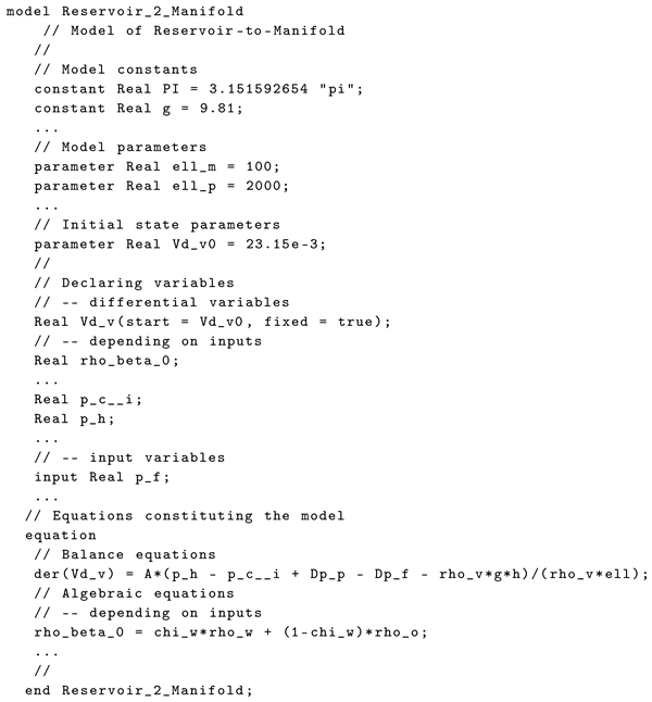
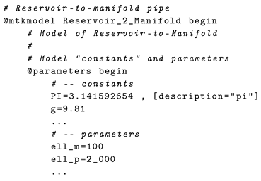
The combined model has been solved using the free languages/tools OpenModelica [10,11] and ModelingToolkit [12] for Julia. To illustrate the similarity between OpenModelica code and a current formulation using ModelingToolkit, the following listing shows parts of the Modelica code for the reservoir heel–to–manifold; to save space, description of quantities is only included for constant

π

to illustrate how it is done:

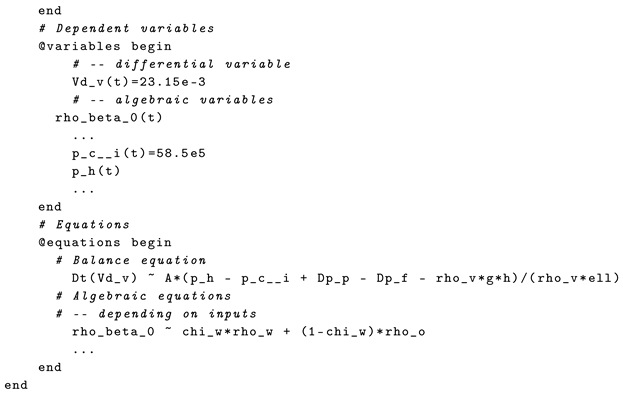
Next, the following listing shows similar parts of the ModelingToolkit code for the reservoir heel–to–manifold:

These listings show that Modelica code and ModelingToolkit code have a high degree of similarity. A few things to note:

In Modelica, the independent temporal variable has a fixed name (time), and the time differentiation operator has a fixed name (der). In ModelingToolkit, both of these can be freely named by the user. In order to make unit models work together (e.g., in a standard library), it is, however, necessary to standardize on a name for time (commonly t); differentiation can be given a name as, e.g., Dt = Differential(t) or similar.
In Modelica, quantities need to be specified with a type (e.g., Real), and are prepended with a qualifier (e.g., constant, parameter) — except for variables. For Julia and ModelingToolkit, the data type is inferred, unless explicitly stated. In the code above, quantities in MTK are grouped within begin...end blocks in macros (identifiers prepended by @, e.g., @parameters).
Modelica has a simple way to handle implicit algebraic equations, and in many cases an initial guess of the algebraic variable is not required (see variable p_c_ _i in the Modelica code). In ModelingToolkit, initial values for unknowns after structural simplification (“states”) must be provided with numeric values (see variable p_c_ _i in the MTK code).
In ModelingToolkit, initial values of differential variables can be changed outside of the code, hence default values can be written as Vd_v(t)=23.15e-3. In Modelica, only parameters can be changed outside of the code (after compilation), hence a parameter has been defined to hold the default initial value Vd_v(start = Vd_v0, fixed = true.
Modelica uses symbol = for mathematical equality; MTK uses symbol ~ since Julia already uses symbol = for assignment.

The default solver in OpenModelica is excellent, although here it struggled if the model is posed as a DAE formulation with momentum as differential variable. ModelingToolkit can use solvers from the large, high quality DifferentialEquations.jl package [13]. With ModelingToolkit, more thought is currently required when choosing solver, accuracies, etc., compared to OpenModelica. Also, OpenModelica handles step-changes in inputs well, while for the DifferentialEquations.jl solvers, it is often necessary to specify the time points where step changes occur. On the other hand, the solutions from ModelingToolkit include interpolation functions, which yields smooth solutions with considerably fewer data points than for Modelica.

Results presented in Section 5 compare numerical solutions for the Reservoir heel–to–Manifold system for ModelingToolkit vs. OpenModelica.

OpenModelica’s support for linearization and plotting can be accessed from Julia via the OMJulia API [14]. ModelingToolkit is integrated in the Julia eco-system, with support for linearization, plotting, control systems analysis, random variables, etc., and has overall more possibilities that OpenModelica if further analysis is required.

OpenModelica is currently reported to handle models up to approximately

10^{6}

variables/equations; various conference presentations indicate that ModelingToolkit currently can solve models of up to approximately

10^{5}

variables/equations.15 The model above (Reservoir_2_Manifold) is reported by OpenModelica to have 15 variables (differential+algebraic) and 15 equations. In ModelingToolkit, linear equations with “observed” variables are stripped off from the model (function structural_simplify()) before solving the model. The above Reservoir_2_Manifold model in the listing is reported to have 2 “states” and 2 equations by ModelingToolkit. It is not clear whether the ModelingToolkit claim of

10^{5}

variables/equations is before or after the “observed” variables are stripped off.

Other commonly used languages for scientific computing are MATLAB (commercial) and Python (free). Compared to both of these languages, Julia (free) has a more extensive set of differential equation solvers16. Neither MATLAB nor Python offer equation based modeling languages with library/re-use support such as Modelica or ModelingToolkit; MathWorks do offer Simscape17 (commercial) with MATLAB integration for such use, though.

5. Results

5.1. Reservoir heel to manifold

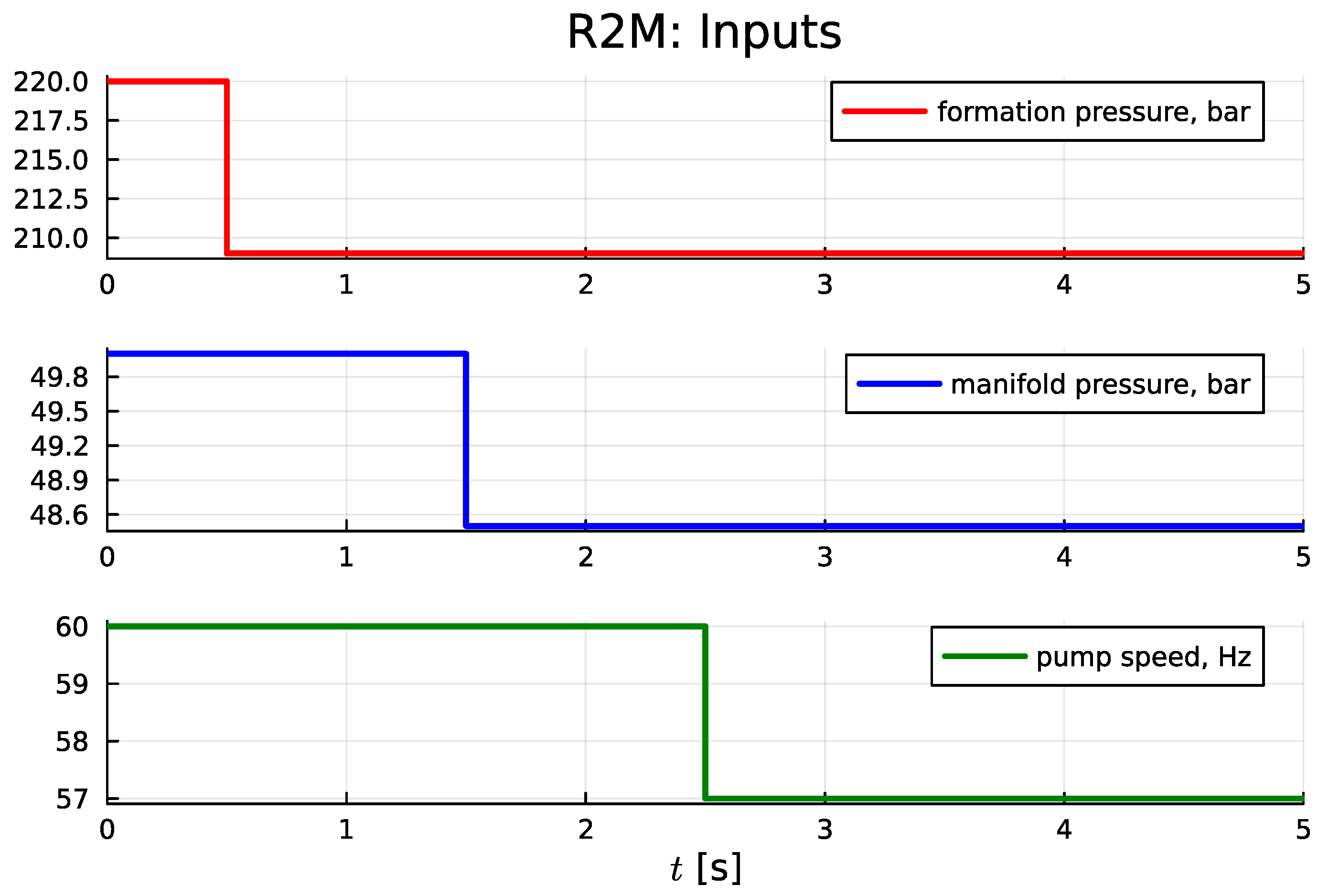
Parameters, initial conditions, and system inputs are given in Appendix A. Figure 6 shows the input variation for the Reservoir heel–to–manifold (R2M) case.

A step change in the formation pressure (red curve) as in Figure 6 is not very realistic; such changes are normally slow. The manifold pressure (blue curve) is not normally an input function, but rather a dependent variable in the overall system as in Section 5.2, and thus also normally varies slowly. The pump speed (green curve) is, however, a control variable, and can change fast. Still, the inputs in Figure 6 will help provide useful information about time constants in the system.

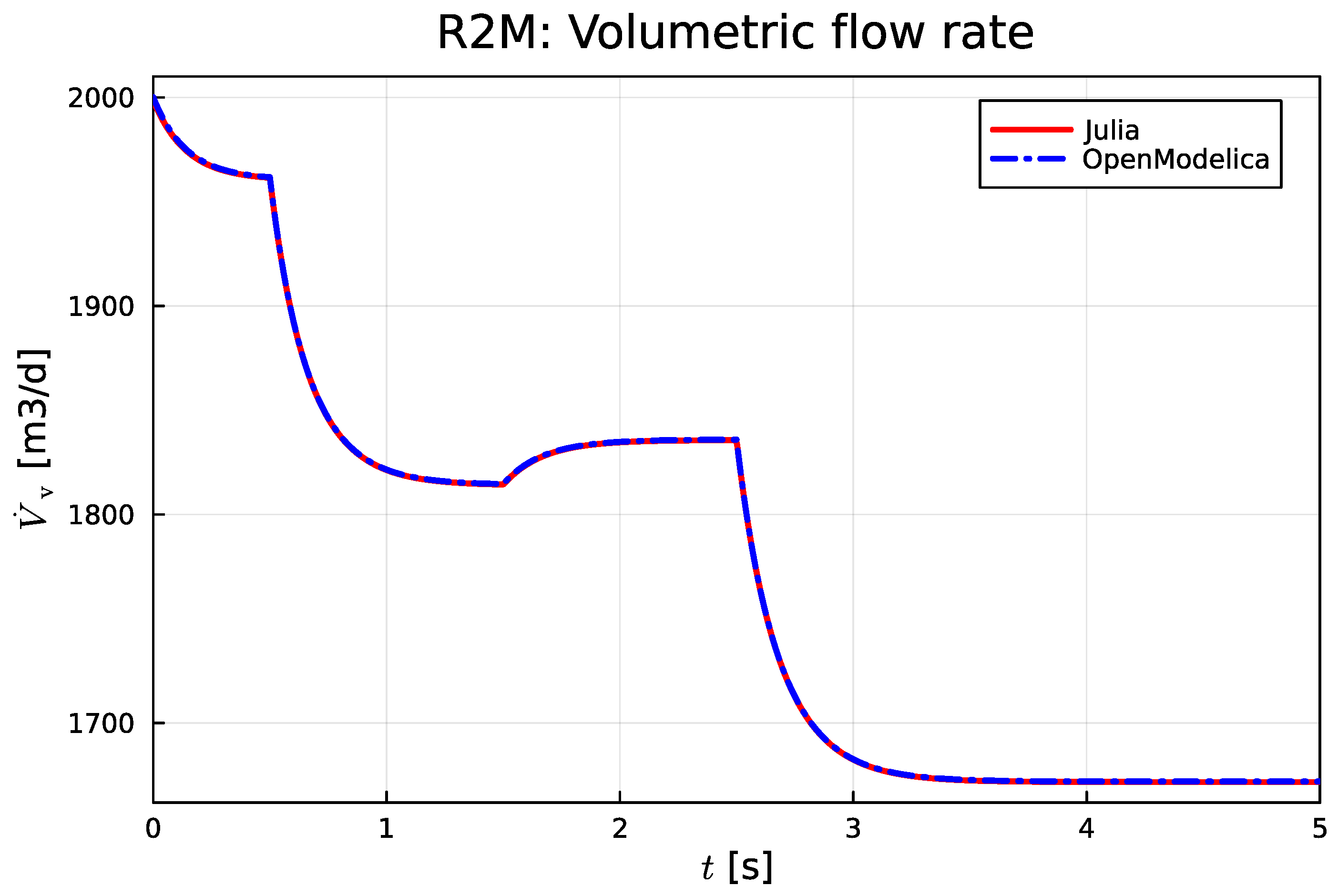
Figure 7 shows the response in (vertical) volumetric flow rate

{\dot{V}}_{v}

, with comparison between Julia (red, solid) and OpenModelica (blue, dash-dot).

An important observation is that the volumetric flow rate is continuous under the step changes in Figure 6. This makes sense, in that the momentum of the fluid (oil-water) is substantial. Time constants are in the range of

0.2

–

0.5 s

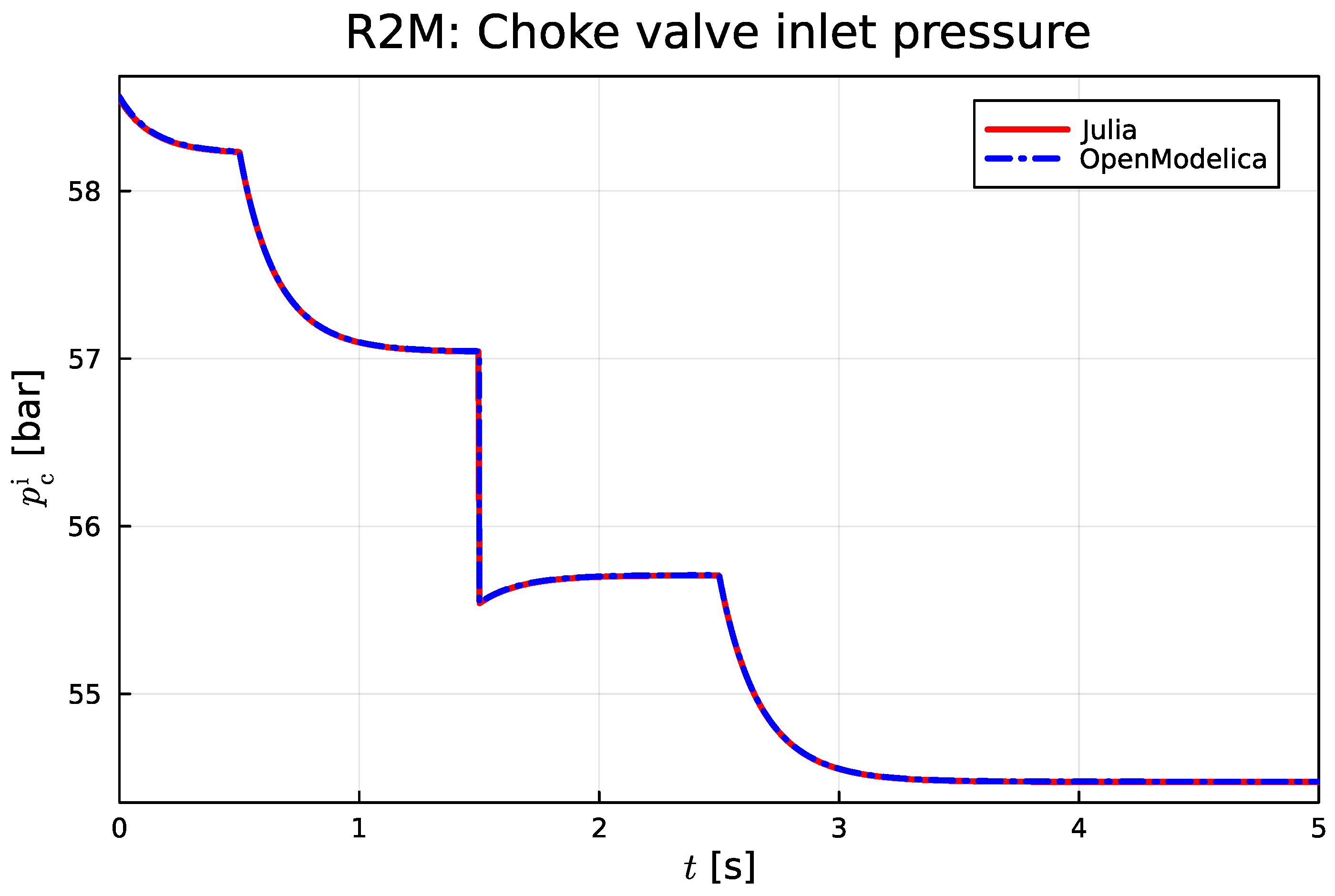
Figure 8 shows the response in the choke valve inlet pressure,

p_{c}^{i}

Observe that the choke valve inlet pressure normally is continuous under step changes, but that it changes discontinuously upon a step change in manifold pressure at

t = 1.5 s

. Again, this makes sense: when the manifold pressure drops, Figure 6, the choke valve inlet pressure must also drop in proportion so that the flow through the valve changes continuously, see Eq. 14.

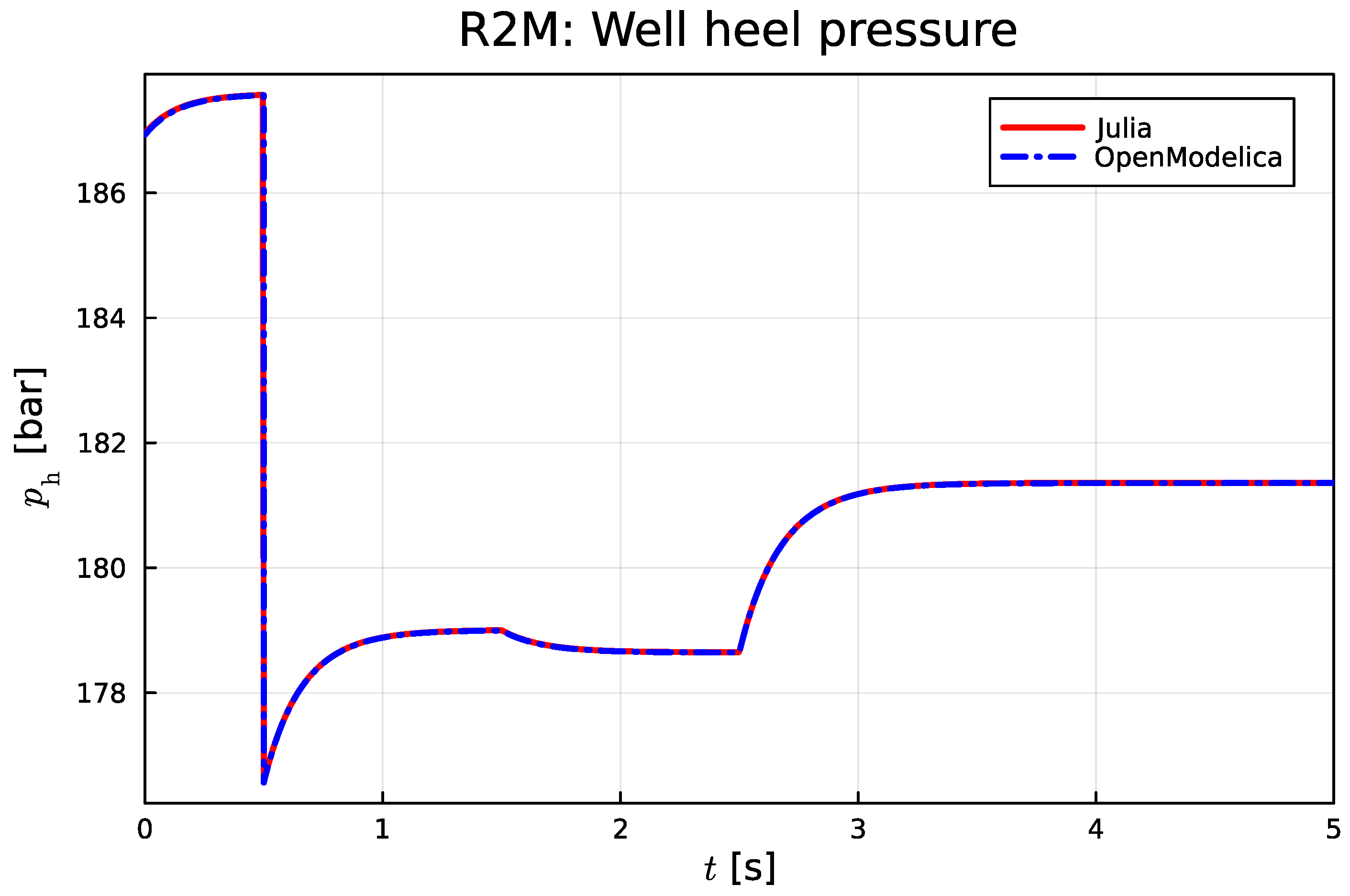
Figure 9 shows the response in the reservoir pressure heel,

p_{h}

As noted, the formation pressure can not change in a step, but if it does, the well heel pressure must also change in proportion (i.e., discontinuously) to maintain continuity in the flow rate.

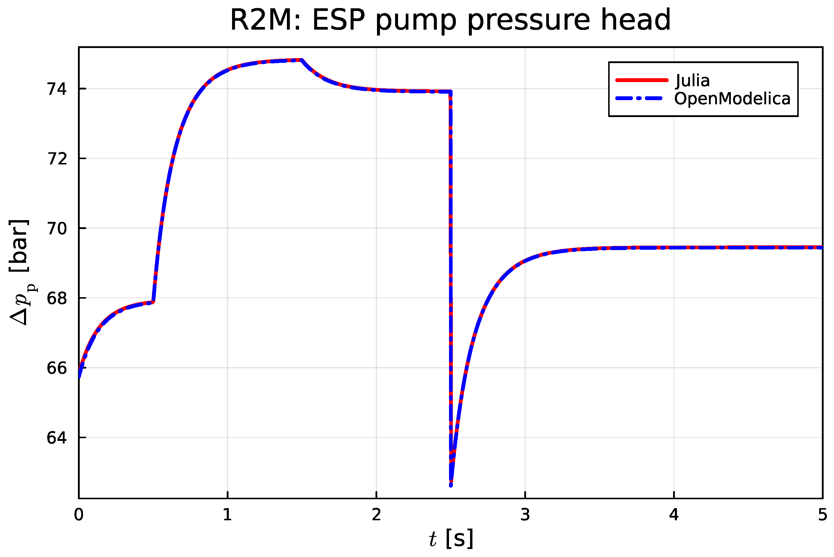
Figure 10 shows the response in the ESP pump pressure head,

Δ p_{p}

Again, the discontinuous change in pump pressure head is due to the step change in the manifold pressure, and the result makes sense.

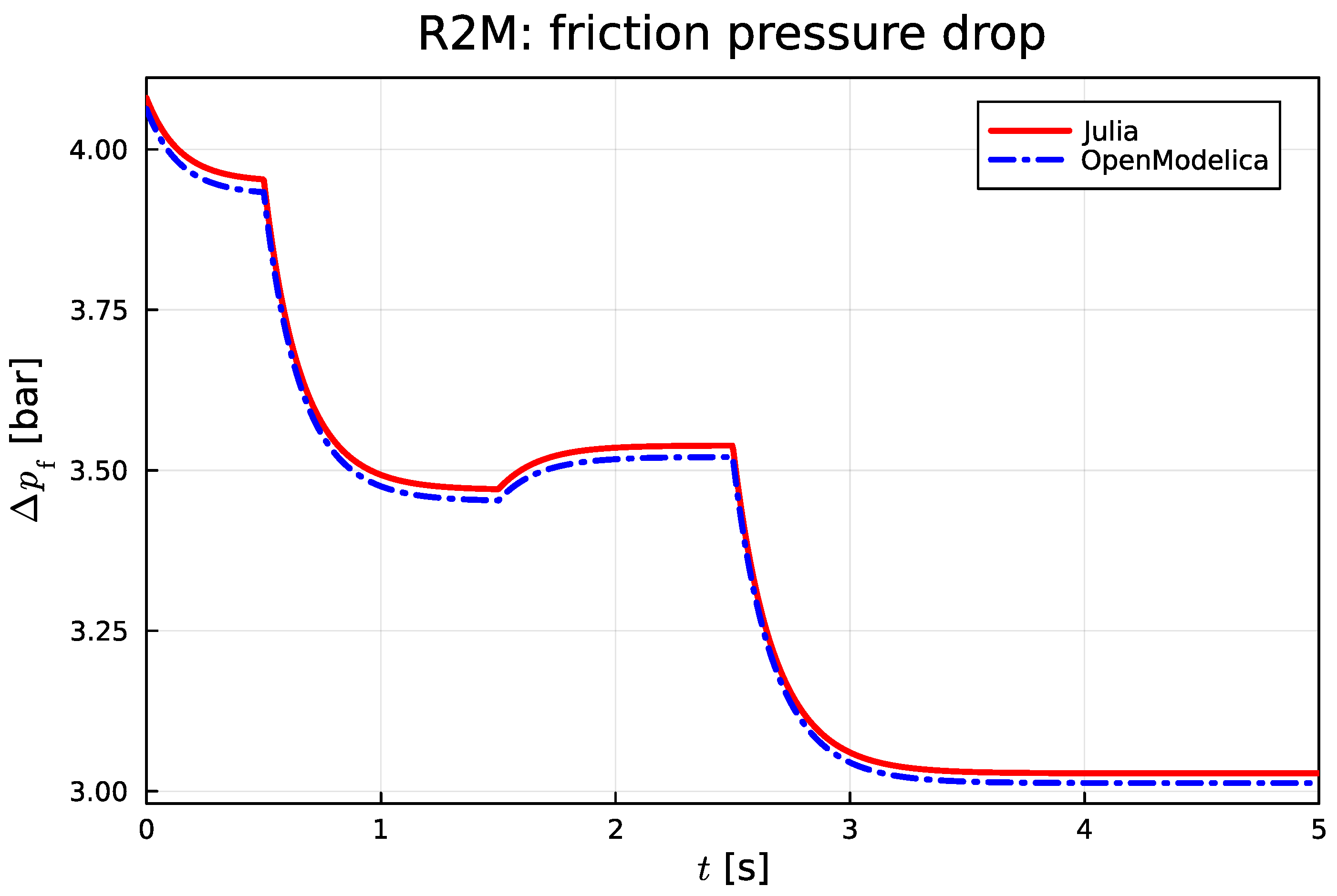
So far, ModelingToolkit/Julia and OpenModelica have given (seemingly) identical simulation results, Figure 7, Figure 8, Figure 9 and Figure 10. Figure 11 shows the pipe friction loss,

Δ p_{f}

It is interesting to contrast the magnitude of the friction loss in Figure 11 and how much smaller it is than the pressure boost in the ESP, Figure 10. Obviously, if a more realistic viscosity model had been used, and in particular if emulsification occurs [8], the friction pressure drop might increase considerable with an unfortunate mixing fraction of oil and water.

Apart from this, it is interesting to observe a slight discrepancy between the result from ModelingToolkit/Julia and OpenModelica in this case. This discrepancy is maintained during a multitude of tests with different solvers and accuracy for the DifferentialEquation.jl solvers [13] and the solvers supported by OpenModelica. It seems like there is a minor discrepancy at

t = 0

for

Δ p_{f}

, which propagates throughout the solution. Because the codes and initial conditions are the same for both implementations, a natural suspicion is that the difference is due to different handling of the implicit algebraic equation at initial time, and that

Δ p_{f}

is rather sensitive to such an inaccuracy.

5.2. Reservoir heel to separator

Parameters, initial conditions, and system inputs are given in Appendix A. For vertical pipe #2, scaling pump head

h_{p, 0}

is set to 80% of the value suggested in Appendix A. For this more complete system (2 vertical pipes, one horizontal transport pipe), there is no observed difference between the solution from ModelingToolkit/Julia and OpenModelica.

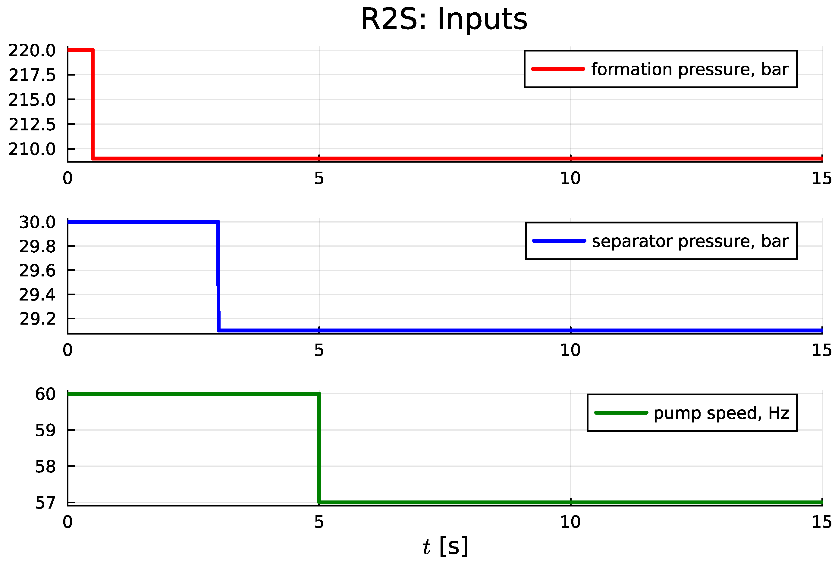
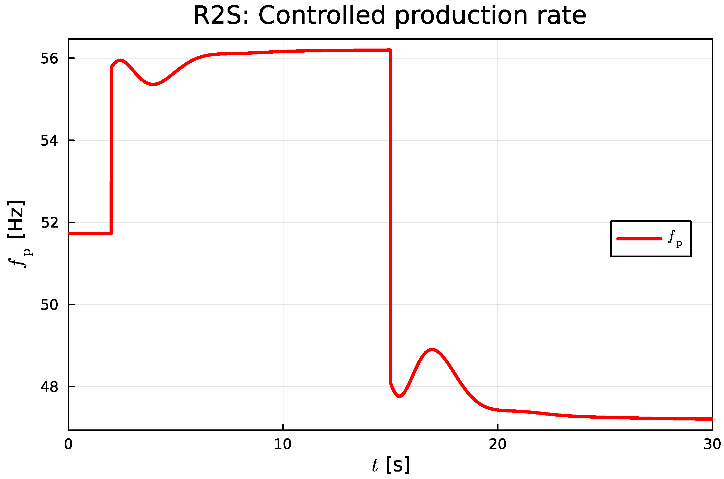
Figure 12 shows the input variation for the Reservoir heel–to–separator (R2S) case; because of slower dynamics for this larger system, the locations of the step changes have been changed, and the step change in the manifold pressure (Figure 6) has been replaced by a step change in the separator pressure (Figure 12).

For comments on formation pressure and pump speed inputs, see Section 5.1. Although the separator pressure is not normally an input function, there may be action applied to the separator that may create relatively quick changes in the separator pressure.

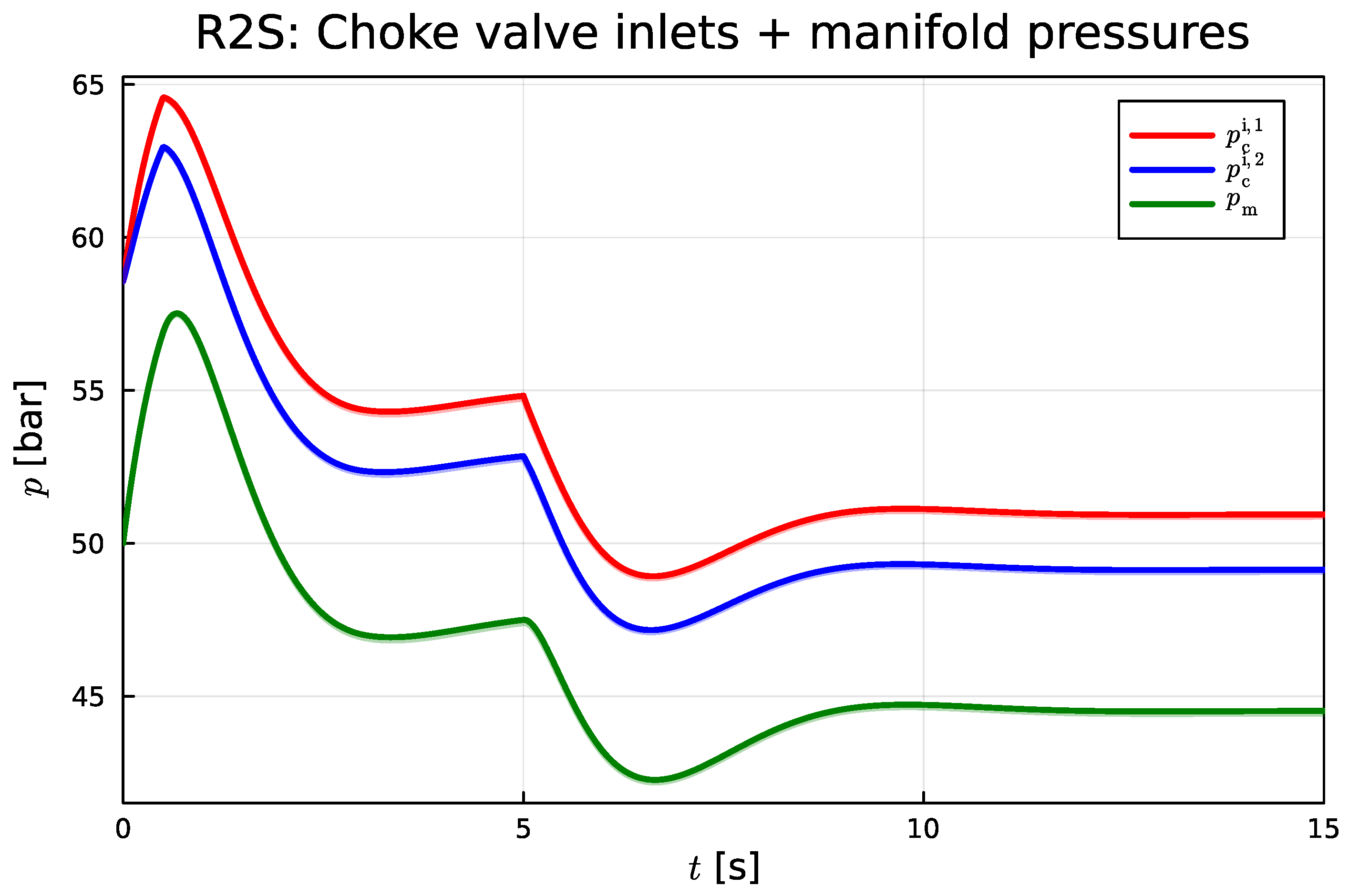
Figure 13 shows the pressures in front of the choke valves for the vertical pipes, as well as the manifold pressure.

Figure 13 demonstrates the positive pressure drop over the choke valves, and that they are different for the two valves (

Δ p_{c}^{j} = p_{c}^{i, j} - p_{m}

). Therefore, one should expect different flows through the two valves. Because the manifold pressure is a dependent (dynamic) variable in this case, there is no discontinuity in the pressures of Figure 13.

Figure 14 displays the pressure increase over the ESP pumps in the two vertical pipes.

In this figure, the sudden drop in

Δ p_{p}

is due to a sudden change in the pump speed

f_{p}

, and is thus realistic.

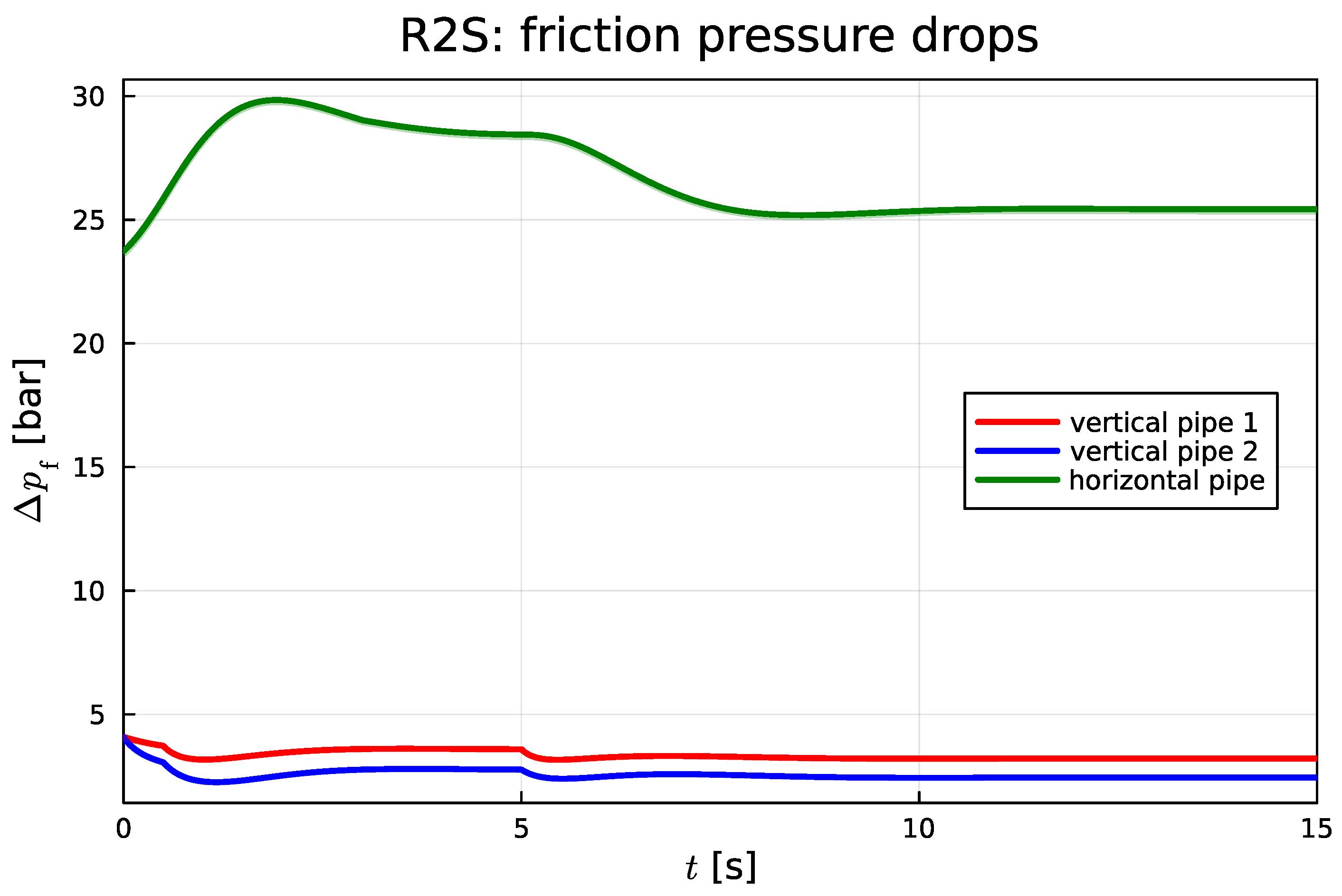
Figure 15 shows the friction pressure drops in the two vertical pipes and in the horizontal pipe.

Here, the interesting thing is that there is no visible difference between OpenModelica and Julia solution of

Δ p_{f}

for the three pipes; confer Figure 11. Of course, this could be due to the zoomed-out view, but also on close inspection of

Δ p_{f}

for the initial few seconds for vertical pipe 1, there is virtually no difference.

The resulting time constants and overall behavior in Figure 13, Figure 14 and Figure 15 are similar to those in Sharma [3]. Particularly in Figure 13 and Figure 14, some oscillatory behavior/overshoot is noticeable. This is to be expected due to the elasticity of the oil/water mixture with the given non-zero value of isothermal compressibility

β_{T}

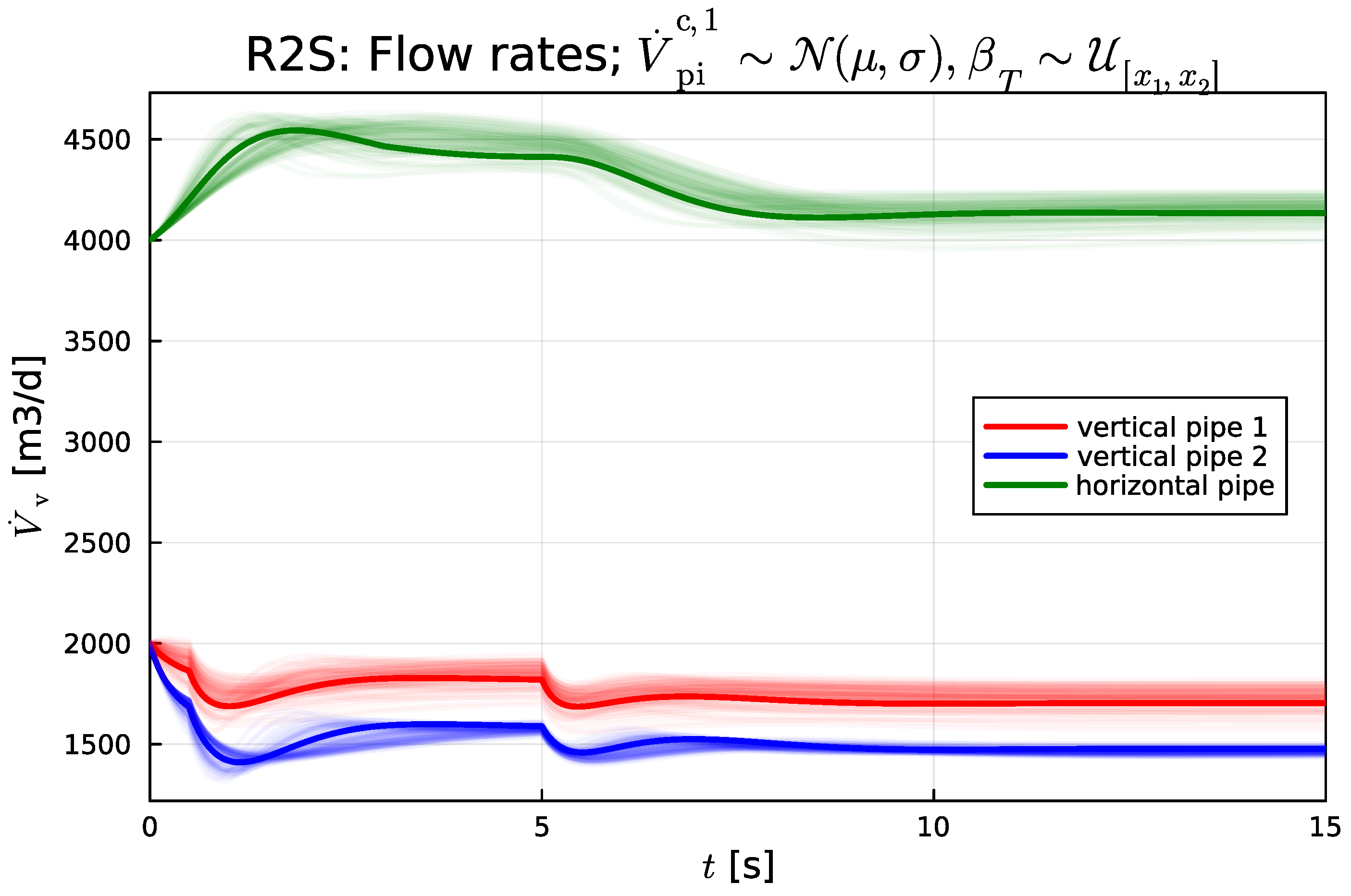
Figure 16 shows vertical flow rates from reservoir to manifold in the two pipes, as well as the flow from manifold to separator (thick, solid lines), and the effect of uncertain productivity indices in Well 1,

{\dot{V}}_{pi}^{c, 1} \sim N (7 \cdot 10^{- 4}, 10^{- 4})

, and uncertain isothermal compressibility in the petroleum fluid,

β_{T} \sim U_{[0.3 / 1.5 \cdot 10^{9}, 3 / 1.5 \cdot 10^{9})]}

ModelingToolkit has support for efficient Monte Carlo studies; this is comparatively more complicated using Modelica + OMJulia.

5.3. Linearized model

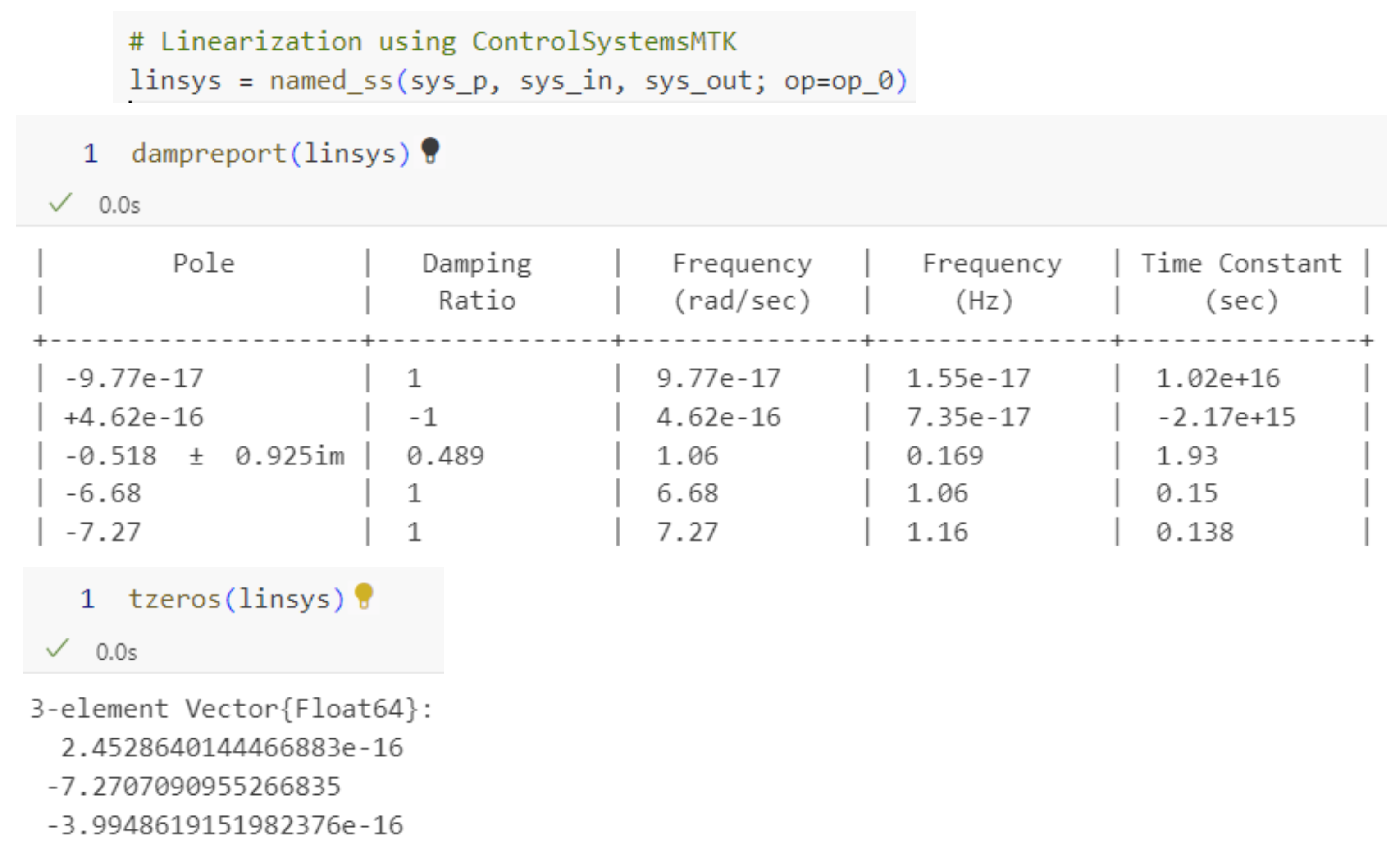
ModelingToolkit.jl has good support for linearization of models. To linearize a system, it is necessary to provide a model where the inputs have not been defined (sys_p in Figure 17), a vector of input variables (sys_in), a vector of output variables (sys_in), and an operating point (keyword op, value op_0). If the ModelingToolkitStandardLibrary.jl (similar to Modelica’s Standard Library) is used, alternatively, some “virtual” inputs/outputs can be added in the form of Analysis Points which simplifies linearization; this is not discussed further here.

In Figure 17, linearization is performed using the named_ss function in ControlSystemsMTK.jl, which has similar arguments as function linearize in ModelingToolkit.jl.

Figure 17 suggests 6 poles/states in the system, and 3 transmission zeros. Obviously, the system has 4 states/differential variables (flow rates

{\dot{V}}_{v}

for each of the vertical pipes, pressure

p_{m}

for the manifold, and flow rate

{\dot{V}}_{t}

for the horizontal transport pipe). Comparing poles and zeros, one might suspect that two spurious/“infinitesimal” poles have been added together with two spurious/“infinitesimal” zeros, and that canceling out the tiny poles and zeros should give the correct transfer function. Observe also that there is a finite zero at

- 7.27

that cancels out one of the 4 true eigenvalues.

It is possible to write one’s own linearization code using a (symbolic) Jacobian function applicable to ModelingToolkit.jl models. If one assumes that the original model is a DAE of index 0 or 1, this will indeed give the correct transfer function with 4 states (and one zero that cancels out one of the eigenvalues). Why does ModelingToolkit.jl produce spurious additional poles/zeros? Possibly because the linearization algorithm in ModelingToolkit.jl makes no assumption of the index of the DAE, thus producing the two spurious “infinitesimal” poles/zeros.

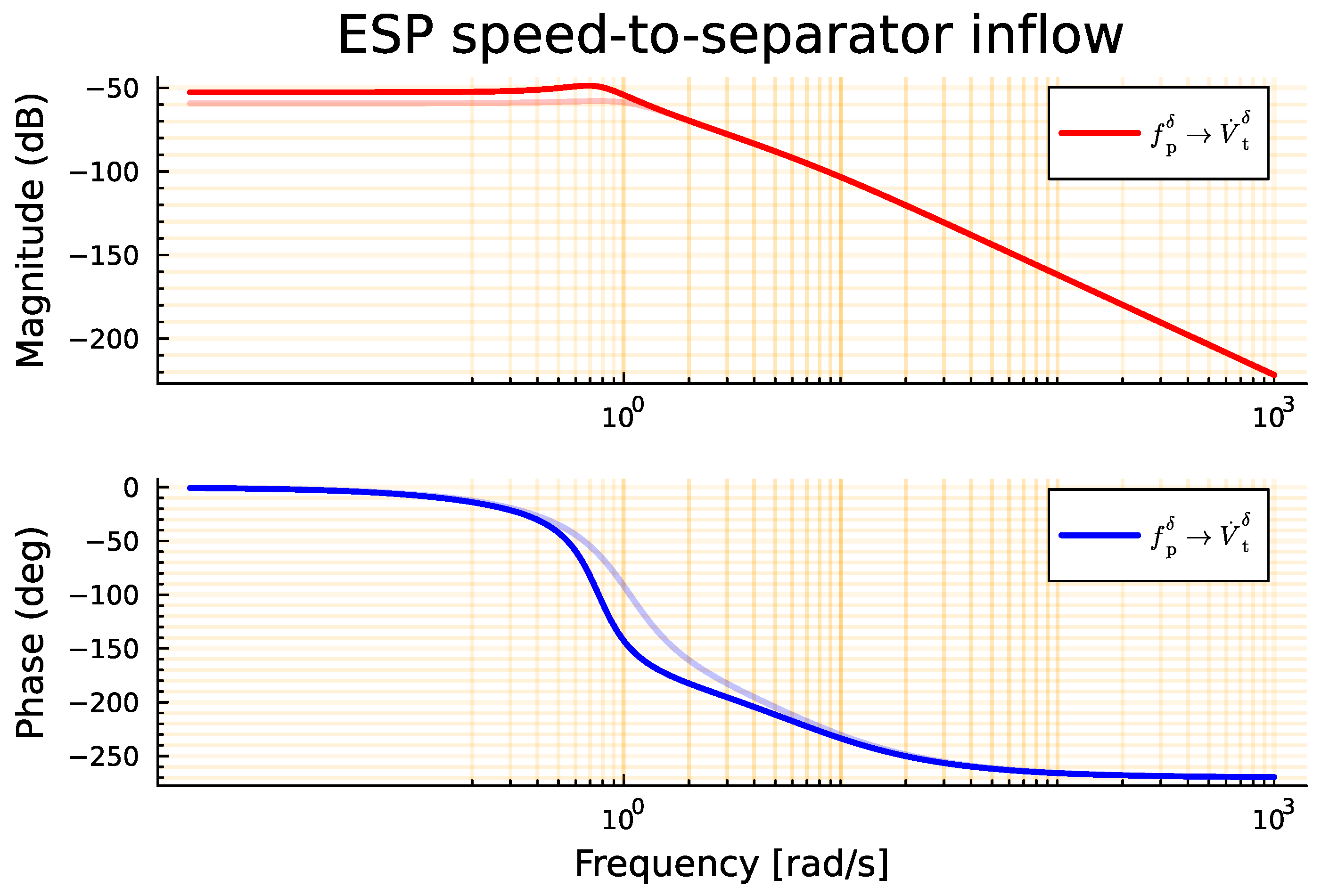
Figure 18 shows the Bode plot of the transfer function from ESP rotational speed (

f_{p}

)18 to flow rate into the separator (

{\dot{V}}_{t}

), as found using Julia + ModelingToolkit.jl based on the transfer function provided by the system in Figure 17. Package ControlSystems.jl also has a function balance_statespace() which in combination with minimal realization provides a transfer function with 3 poles or 1 time constant and one damped resonator,

P (s) \approx \frac{1.094 \cdot 10^{- 3}}{(1 + 0.15 s) (1 + 2 \cdot 0.489 \frac{s}{1.06} + {(\frac{s}{1.06})}^{2})};

(60)

see pale curves in Figure 18.

It is possible to instead use Modelica+OMJulia for linearization, and then use ControlSystems.jl for Julia [similar capabilities as MATLAB’s Control Toolbox] for plotting and analysis/design. However, control analysis and design is simpler to do if a Julia set-up is used also for modeling and simulation.

5.4. Single-loop controller tuning

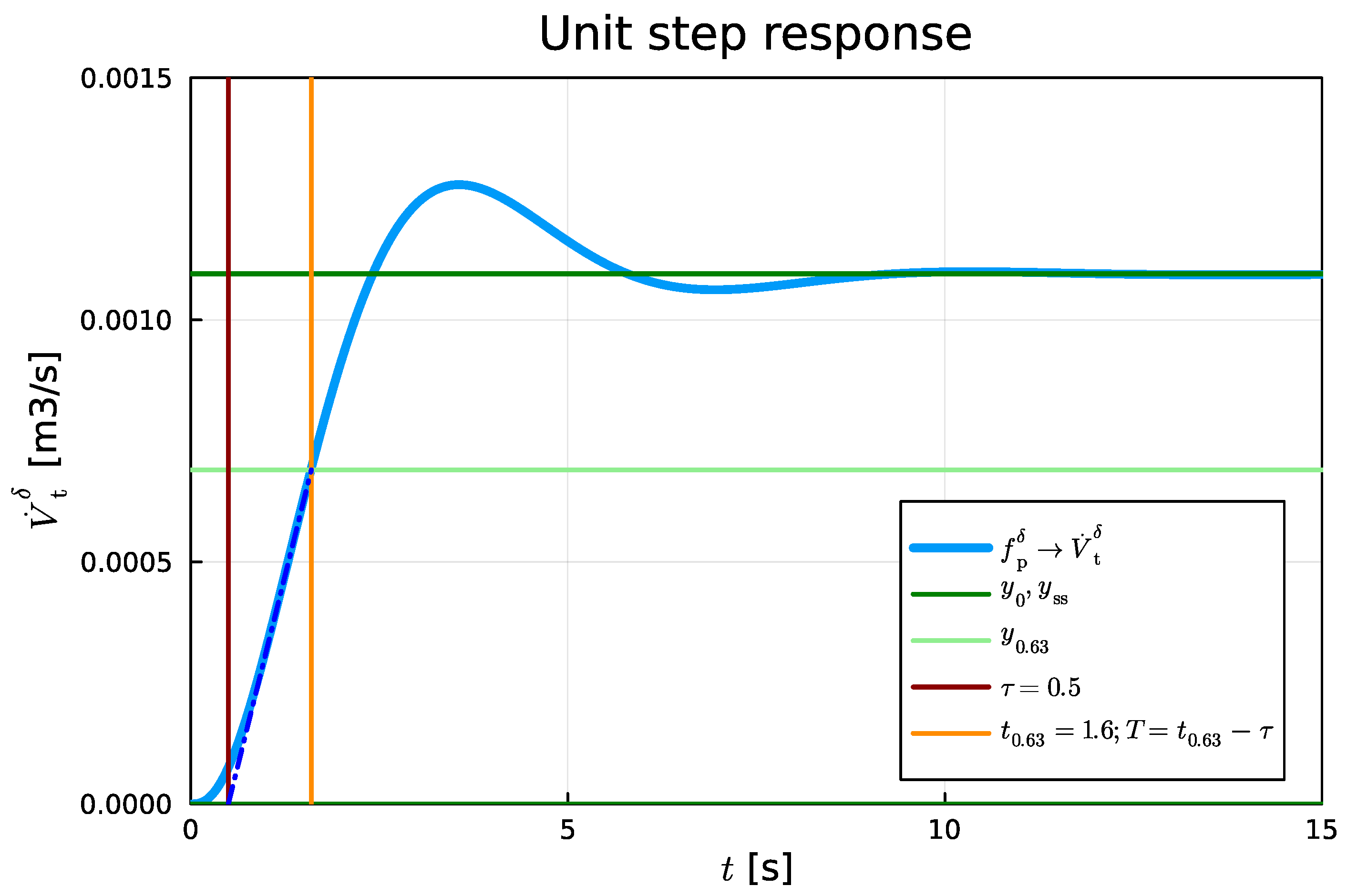
Figure 19 shows a unit step response for the linearized model using convenience function step() in package ControlSystems.jl.

A crude approximation of the system is read off Figure 19 as the plant transfer function

P_{\approx} (s)

P_{\approx} (s) = K \frac{exp (- τ s)}{s}

(61)

with

\begin{matrix} K & \approx 6.27 \cdot 10^{- 3} \\ τ & \approx 0.5 . \end{matrix}

A PI controller

C (s) = K_{p} \frac{1 + T_{i} s}{T_{i} s}

(62)

based on Skogestad’s method [15,16,17] is used with

\begin{matrix} T_{ℓ} & = 1.3 \cdot τ \end{matrix}

(63)

\begin{matrix} κ & = 4 \end{matrix}

(64)

\begin{matrix} K_{p} & = \frac{1}{K (τ + T_{ℓ})} \end{matrix}

(65)

\begin{matrix} T_{i} & = κ (τ + T_{ℓ}); \end{matrix}

(66)

where tuning parameters are:

T_{ℓ}

, closed loop time constant;

κ

, integral time modifier.

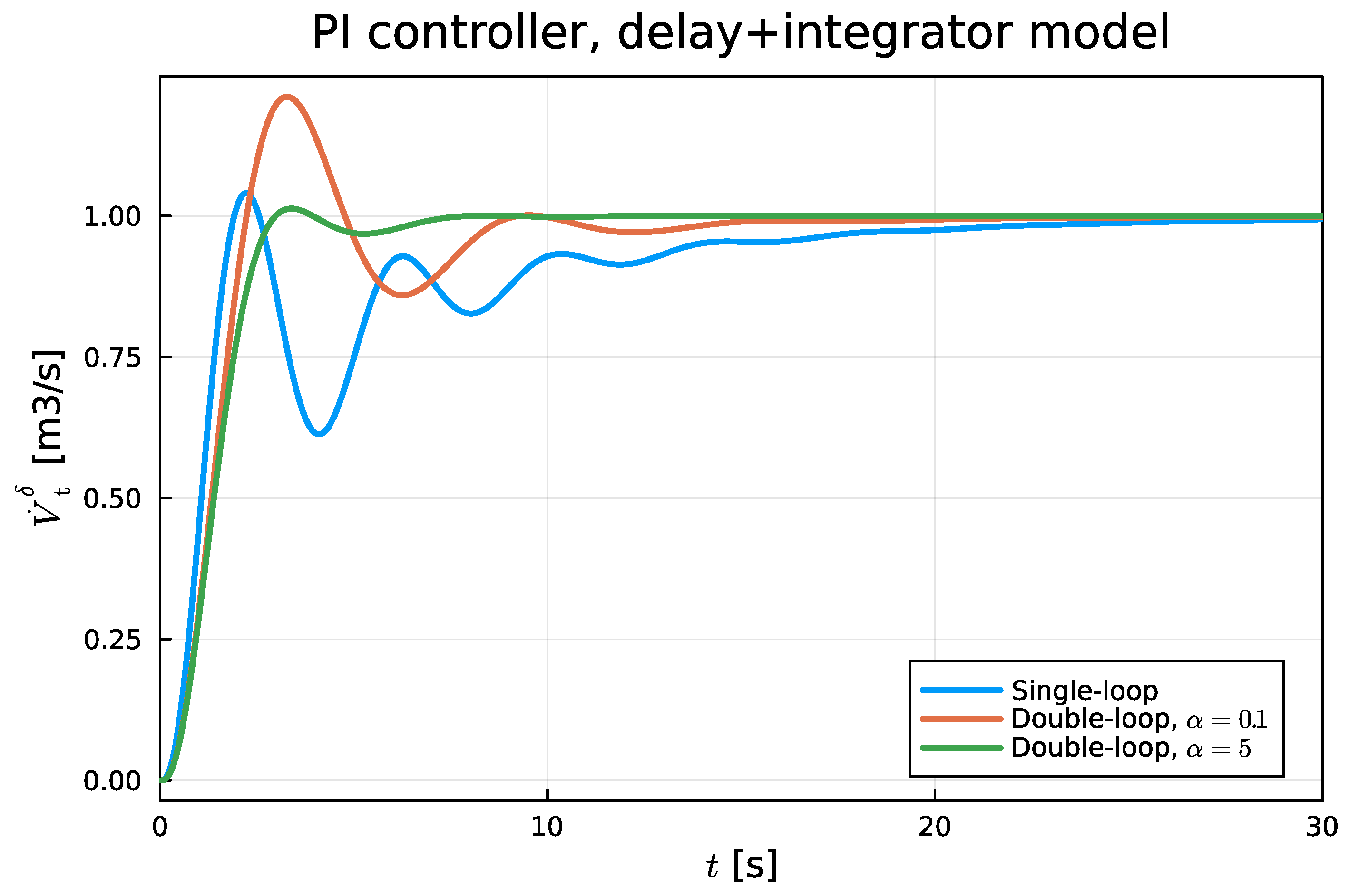
Figure 20 shows a unit reference step response for the closed loop system [blue line]; here, utility function feedback(P*C) has been used to construct the closed-loop system. Observe that the closed loop time constant

T_{ℓ}

is not achieved, and that the resulting system is rather oscillatoric.

The reason for the oscillatoric behavior is that single-loop tuning methods are not designed for oscillatoric systems as the one in Eq. 60.

5.5. Double-loop controller tuning

In order to better handle the oscillatoric behavior of the system, which has generic form

P_{ζ} (s) = \frac{K}{(1 + T_{1} s) (1 + 2 ζ \frac{s}{ω_{0}} + {(\frac{s}{ω_{0}})}^{2})},

(67)

an idea of Nandong [18] is pursued, where the control signal is split into an “inner” control signal

u_{i} = - C_{i} (s) y

(68)

and an “outer” control signal

u_{o}

u = u_{i} + u_{o}

(69)

where first

C_{i}

is designed to reduce the oscillations in the system.

Consider the following proper inner controller

C_{i} (s) = K_{c}^{i} \frac{1 + T_{1} s}{1 + α T_{1} s};

(70)

Inserting controller Eq. 68 into

y = P_{ζ} (s) u

with u as in Eq. 69 and

P_{ζ} (s)

as in Eq. 67 leads to,

\begin{matrix} y & = P_{ζ} (s) u = P_{ζ} (s) (- C_{i} (s) y + u_{o}) \\ ⇓ \\ (1 + P_{ζ} (s) C (s)) y & = P (s) u_{o} \end{matrix}

which after some re-arrangement gives:

(1 + \frac{K K_{c}^{i}}{1 + α T_{1} s} + 2 ζ \frac{s}{ω_{0}} + {(\frac{s}{ω_{0}})}^{2}) y = \frac{K}{1 + T_{1} s} u_{o} .

For small values of

α

α \to 0

\begin{matrix} (1 + K K_{c}^{i}) + 2 ζ \frac{s}{ω_{0}} & + {(\frac{s}{ω_{0}})}^{2} = (1 + K K_{c}^{i}) \times \\ \dots \times (1 + 2 ζ_{i} \frac{s}{ω_{i}} + {(\frac{s}{ω_{i}})}^{2}) \end{matrix}

where closed loop damping

ζ_{i}

given by

\begin{matrix} ζ_{i} & = ζ / \sqrt{1 + K K_{c}^{i}} \\ ⇓ \\ K_{c}^{i} & = \frac{{(ζ / ζ_{i})}^{2} - 1}{K} . \end{matrix}

(71)

A design procedure could thus be:

Specify inner loop damping, $ζ_{i} \geq 1$ to provide (over-) damping.
Compute inner gain $K_{c}^{i}$ from Eq. 71.
Choose a “small” value for $α$ to make the above design valid.

We choose

ζ_{i} = 1

, and compute

K_{c}^{i}

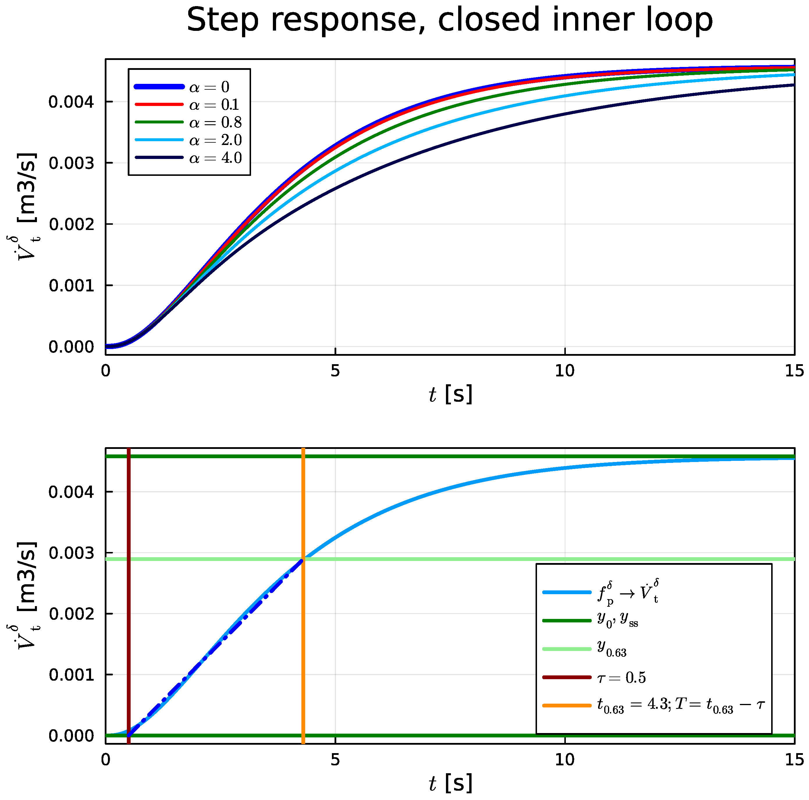
from Eq. 71. Next, closing the loop from

u_{o}

to y where we allow for

α > 0

to have a realizable controller, the step response is as in Figure 21.

Based on closed inner loop with

α = 0.1

as in the lower plot of Figure 21, we find model parameters in the model of Eq. 61 to be:

\begin{matrix} K & \approx 0.762 \cdot 10^{- 3} \\ τ & \approx 0.5 . \end{matrix}

Tuning an outer loop PI controller with Skogestad’s method with an integrator + delay approximation, this time with

T_{ℓ} = 2 \cdot τ

, the result is as in Figure 20, red curve. Although the result is considerable faster than what is achieved with the single-loop controller (same figure, blue curve), the result is surprisingly oscillatoric.

It is interesting to observe that with the same value for

T_{ℓ} = 2 \cdot τ

, and changing

α

from

α = 0.1

α = 5

, this gives a considerably better response, Figure 20, green curve.

5.6. Controller implementation with nonlinear model

The inner loop controller of Eq. 68 with

C_{i} (s)

as in Eq. 70 admits the following state space realization

\begin{matrix} \frac{d z_{i}}{d t} & = - \frac{1}{α T_{1}} z_{i} + y \\ u_{i} & = \frac{K_{c}^{i}}{α^{2} T_{1}} (1 - α) z_{i} - \frac{K_{c}^{i}}{α} y, \end{matrix}

where we must require

α > 0

. The PI controller for the outer loop as in Eq. 62 admits the following state space realization:

\begin{matrix} e & = r - y \\ \frac{d z_{o}}{d t} & = \frac{1}{T_{i}^{o}} e \\ u_{o} & = K_{p}^{o} (e + z_{o}) . \end{matrix}

With

y \leftarrow {\dot{V}}_{t}

as input to the controller together with a reference value

r \leftarrow {\dot{V}}_{t}^{ref}

, the controller produces output

u = u_{i} + u_{o} \to f_{p}

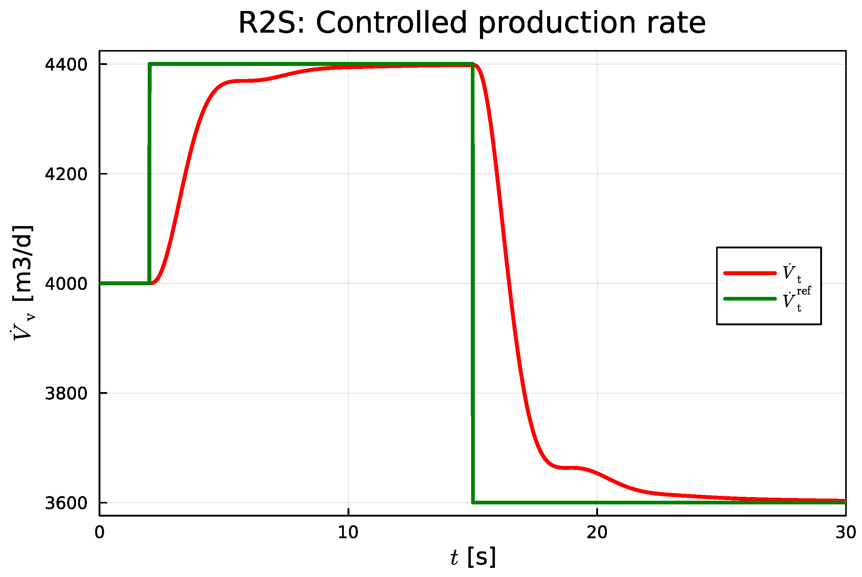
and is straightforward to implement in ModelingToolkit (or Modelica) and connect with the reservoir-to-separator model. Using the inner-outer model with

α = 5

, starting in steady state and injecting a step change in

{\dot{V}}_{t}^{ref}

gives the response as in Figure 22.

The response in Figure 22 [red curve] is similar to the corresponding response [green curve] in Figure 20.

The response in Figure 22 is achieved with an ESP pump speed as in Figure 23.

In reality, it is not possible to “require” more production than the reservoir can produce. To handle this correctly, a more complex interaction with the reservoir than the productivity index model is required.

6. Conclusions

Sharma and Glemmestad [1], Sharma [3] provided a novel model of an ESP-lifted oil production system from reservoir to separator. In Lie [2], the model of Sharma and Glemmestad [1] was provided with a more structured model development, and with dimensionless equipment models. Also, some information that is difficult to find in the original publications (e.g., ESP model parameters) was included. A basic comparison of equation based modeling languages Modelica and ModelingToolkit for Julia was given.

Here, the work in Lie [2] is extended in several directions: (i) a couple of model typos in [2] are corrected, (ii) some more fluid details are given, (iii) more details of the ESP model is provided for reference (max/min flow rates, power consumption, efficiency), (iv) an extended discussion of pump control inputs is included, (v) a more thorough discussion is given of advantages with dimensionless models, (vi) a more detailed comparison of model implementation in Modelica vs. ModelingToolkit is provided, (vii) with a comparison of simulation results using OpenModelica vs. ModelingToolkit with Julia, (viii) more simulation results are included for reference, (ix) model linearization using ModelingToolkit with ControlSystems.jl for Julia is discussed, (x) controller tuning for the linearized model is illustrated using Skogestad’s method applied to a simple integrator+time delay approximation, as well as a double-loop design to dampen oscillations, (xi) the double-loop controller is applied to the nonlinear ModelingToolkit model to confirm the controller tuning. Model parameters, inputs, and initial states are provided in Appendix A.

A key difference between the model description here and the original one [1] is the focus on dimensionless models, which greatly reduces the chance of errors. The inclusion of the ESP power consumption model and flow rate constraints/best-efficiency-point for reference, makes it possible with realistic studies of constraints in controller design. Although not implemented here, an extension of more realistic pump control inputs by inclusion of the pump-motor aggregate moment of inertia is discussed. For some systems, such an extension may be of interest.

Both Modelica and ModelingToolkit are suitable and free languages for structured model development. Modelica is a mature language and a good choice, while ModelingToolkit is a more general language with an extensive eco-system. Model implementation is very similar for the two languages; ModelingToolkit does support more general model classes such as distributed models, stochastic models, etc., and has an extensive tool-set for control design, optimization, model fitting, etc. The numeric solutions are virtually identical for the two implementations; a minor discrepancy in friction pressure loss in one case is most likely due to a difference in handling implicit algebraic equations.

Model linearization is provided by both OpenModelica and ModelingToolkit for Julia; in the case of ModelingToolkit, the eco-system of Julia for further analysis and design can directly be used, while for OpenModelica, the linearization can be carried out via a script language API (e.g., from Julia, Python, or MATLAB) and analyzed in the host language.

For illustration purpose, linearization of the system from ESP pump speed to volumetric separator flow using ModelingToolkit/ControlSystems.jl is carried out in Julia. Then, several linear controllers are developed based on Skogestad’s method for an integrator+time delay model approximation, as well for a double-loop controller to dampen oscillations in the system caused by the compressible fluid in the manifold. A re-tuning of the double-loop controller with Skogestad’s method in the outer loop gives best performance. Implementation of the best controller in ModelingToolkit confirms that the linear controller works well with the nonlinear reservoir-to-separator system under the simulated experimental conditions.

The model development and discussion indicates a number of possible extensions such as (a) more realistic properties (density, viscosity), (b) allowing for distributed density along pipes19, (c) adding a more realistic system for water dilution in the manifold, (d) inclusion of valves in manifold–separator pipes, (e) integration with reservoir models, (f) use for advanced control design with constraints, (g) use for optimization, (h) integration with a reservoir model to study how to handle stiffness, and more Such extensions will give more insight into the industrial usefulness of the model.

Funding

The economic support from The Research Council of Norway and Equinor ASA through Research Council project “308817 —Digital wells for optimal production and drainage” (DigiWell) is gratefully acknowledged.

Acknowledgments

Information/data for the original paper [1] provided by dr. Roshan Sharma and Ph.D. student Kushila Jayamanne, both at University of South-Eastern Norway, is gratefully acknowledged.

Conflicts of Interest

The author declares no conflict of interest. The background information for the study predates the funded project, and is openly available. Although the study is relevant to the funded project [DigiWell], the funders had no role in the design of the study; in the collection, analyses, or interpretation of data; in the writing of the manuscript; or in the decision to publish the results.

Abbreviations

The following abbreviations are used in this manuscript:

CFD	Computational Fluid Dynamics
ESP	Electric Submersible Pump
MTK	ModelingToolkit
R2M	Reservoir heel-to-Manifold
R2S	Reservoir heel-to-Separator

Appendix A. Parameters and Operating Conditions

Parameters for petroleum fluid, nominal vertical pipes, and nominal manifold+horizontal pipe are given in Table A1, Table A2 and Table A3. Initial states are given in Table A4, while input functions are given in Table A5.

Table A1. Parameters: petroleum liquid.

Parameter
$β_{T} = \frac{1}{1.5 \cdot 10^{9}} \approx 6.67 \cdot 10^{- 10} P a^{- 1}$
$p_{0} = 1 bar$
$ρ_{o} = 900 kg / m^{3}$
$ρ_{w} = 1000 kg / m^{3}$
$χ_{w} = 0.35$
$ρ_{0} = χ_{w} ρ_{w} + (1 - χ_{w}) ρ_{o}$
$χ_{w}^{m} = 0.5$
$ρ_{0}^{m} = χ_{w}^{m} ρ_{w} + (1 - χ_{w}^{m}) ρ_{o}$
$ν_{o} = 100 cst = 100 \cdot 10^{- 6} m^{2} / s$
$ν_{w} = 1 cst = 10^{- 6} m^{2} / s$

Table A2. Parameters: vertical pipe.

Parameter
$ℓ^{-} = 100 m$
$ℓ^{+} = 2000 m$
$d = 0.1569 m$
$ϵ = 0.0018 inch = {45.7}^{-} m = 45.7 \cdot 10^{- 6} m$
${\dot{V}}_{min, 0} = 14.43 \cdot 10^{- 3} m^{3} / s$
${\dot{V}}_{η, 0} = 19.83 \cdot 10^{- 3} m^{3} / s$
${\dot{V}}_{max, 0} = 25.24 \cdot 10^{- 3} m^{3} / s$
$h_{p, 0} = 1210.6 m$
$f_{p, 0} = 60 Hz$
${\dot{V}}^{ς} = 1 m^{3} / s$
$a_{1} = - 37.57$
$a_{2} = 2.864 \cdot 10^{3}$
$a_{3} = - 8.668 \cdot 10^{4}$
${\dot{W}}_{p, 0}^{m} = 167.733 kW$
$b_{1} = 52.12$
$b_{2} = - 768.7$
$b_{3} = 38.544 \cdot 10^{3}$
$b_{4} = - 1.534 \cdot 10^{6}$
${\dot{m}}_{v}^{c} = 25.9 \cdot 10^{3} kg / h$
$f (u_{v}) = \{\begin{matrix} 0, & u_{v} \leq 0.05 \\ \frac{11.1 u_{v} - 0.556}{30}, & 0.05 < u_{v} \leq 0.5 \\ \frac{50 u_{v} - 20}{30}, & 0.5 < u_{v} \leq 1 \end{matrix}$
$p^{ς} = 1 bar$
$ρ^{ς} = 1000 kg / m^{3}$
${\dot{V}}_{pi}^{c} = 7 \cdot 10^{- 4} m^{3} / s$

Table A3. Parameters: manifold+horizontal pipe.

Parameter
$ℓ_{m} = 500$
$d_{m} = 0.1569$
$ℓ_{t} = 4000 m$
$d_{t} = 0.1569 m$
$ϵ = 0.0018 inch = {45.7}^{-} m = 45.7 \cdot 10^{- 6} m$
$Δ p_{bp, 0} = 10 bar$
$f_{bp, 0} = 60 Hz$

Table A4. Nominal initial states.

Variable
${\dot{V}}_{v} (t = 0) = 2000 m^{3} / d \approx 0.02315 m^{3} / s$
$p_{m} (t = 0) = 50 bar = 50 \cdot 10^{5} Pa$
${\dot{V}}_{t} (t = 0) = 2000 m^{3} / d \approx 0.02315 m^{3} / s$

Table A5. Nominal inputs.

Variable
$p_{f} (t) = \{\begin{matrix} 220 bar, & t < 0.5 s \\ 0.95 \cdot 220 bar, & t \geq 0.5 s \end{matrix}$
$p_{s} (t) = \{\begin{matrix} 30 bar, & t < 3 s \\ 0.97 \cdot 30 bar, & t \geq 3 s \end{matrix}$
$f_{p} (t) = \{\begin{matrix} 60 Hz, & t < 5 s \\ 0.95 \cdot 60 Hz, & t \geq 5 s \end{matrix}$
$u_{v} (t) = 1.0$
$f_{bp} = 60 Hz$

References

Sharma, R.; Glemmestad, B. Modeling and Simulation of an Electric Submersible Pump Lifted Oil Field. International Journal of Petroleum Science and Technology 2014, 8, 39–68. [Google Scholar]
Lie, B. ESP Lifted Oil Field: Core Model, and Comparison of Simulation Tools. Scandinavian Simulation Society 2023, pp. 159–166. [CrossRef]
Sharma, R.Optimal Operation of Gas Lifted and ESP Lifted Oil Fields: An Approach Based on Modeling, Simulation, Optimization and Control. PhD thesis, University of South-Eastern Norway, Kjølnes Ring 56, N-3918 Porsgrunn, Norway, 2014.
Binder, B.J.T.; Pavlov, A.; Johansen, T.A. Estimation of Flow Rate and Viscosity in a Well with an Electric Submersible Pump Using Moving Horizon Estimation. IFAC-PapersOnLine 2015, 48–6, 140–146. [Google Scholar] [CrossRef]
Krishnamoorthy, D.; Bergheim, E.M.; Pavlov, A.; Fredriksen, M.; Fjalestad, K. Modelling and Robustness Analysis of Model Predictive Control for Electrical Submersible Pump Lifted Heavy Oil Wells. IFAC-PapersOnLine 2016, 49–7, 544–549. [Google Scholar] [CrossRef]
Delou, P.d.A.; de Azevedo, J.P.A.; Krishnamoorthy, D.; Jr, M.B.d.S.; Secchi, A.R. Model Predictive Control with Adaptive Strategy Applied to an Electrical Submersible Pump in a Subsea Environment. IFAC PapersOnLine 2019, 52–1, 784–789. [Google Scholar] [CrossRef]
Santana, B.A.; Fontes, R.M.; Schnitman, L.; Martins, M.A.F. An Adaptive Infinite Horizon Model Predictive Control Strategy Applied to an ESP-lifted Oil Well System. IFAC PapersOnLine 2021, 54–3, 176–181. [Google Scholar] [CrossRef]
Justiniano, M.; Romero, O.J. Inversion Point of Emulsions as a Mechanism of Head Loss Reduction in Onshore Pipeline Heavy Oil Flow. Brazilian Journal of Petroleum and Gas 2021, 15, 13–24. [Google Scholar] [CrossRef]
Brkić, D. Review of Explicit Approximations to the Colebrook Relation for Flow Friction. Journal of Petroleum Science and Engineering 2011, 77, 34–48. [Google Scholar] [CrossRef]
Fritzson, P. Principles of Object-Oriented Modeling and Simulation with Modelica 3.3: A Cyber-Physical Approach, second ed.; Wiley-IEEE Press: Piscataway, NJ, 2015.
Fritzson, P.; Pop, A.; Asghar, A.; Bachmann, B.; Braun, W.; Braun, R.; Buffoni, L.; Casella, F.; Castro, R.; Danós, A.; Franke, R.; Gebremedhin, M.; Lie, B.; Mengist, A.; Moudgalya, K.; Ochel, L.; Palanisamy, A.; Schamai, W.; Sjölund, M.; Thiele, B.; Waurich, V.; Östlund, P. The OpenModelica Integrated Modeling, Simulation and Optimization Environment. Proceedings of the 1st American Modelica Conference; LIU Electronic Press, www.ep.liu.se: Cambridge, MA, USA, 2018.
Ma, Y.; Gowda, S.; Anantharaman, R.; Laughman, C.; Shah, V.; Rackauckas, C. ModelingToolkit: A Composable Graph Transformation System For Equation-Based Modeling. arXiv 2021. [Google Scholar] [CrossRef]
Rackauckas, C.; Nie, Q. DifferentialEquations.Jl — A Performant and Feature-Rich Ecosystem for Solving Differential Equations in Julia. Journal of Open Research Software 2017, 5. [Google Scholar] [CrossRef]
Lie, B.; Palanisamy, A.; Mengist, A.; Buffoni, L.; Sjölund, M.; Asghar, A.; Pop, A.; Fritzson, P. OMJulia: An OpenModelica API for Julia-Modelica Interaction. Proceedings of the 13th International Modelica Conference, 2019, pp. 699–708. [CrossRef]
Skogestad, S. Simple Analytic Rules for Model Reduction and PID Controller Tuning. Journal of Process Control 2003, 13, 291–309. [CrossRef]
Skogestad, S. Simple Analytic Rules for Model Reduction and PID Controller Tuning. Modeling, Identification and Control: A Norwegian Research Bulletin 2004, 25, 85–120. [Google Scholar] [CrossRef]
Haugen, F. Comparing PI Tuning Methods in a Real Benchmark Temperature Control System. Modeling, Identification and Control 2010, 31, 79–91. [Google Scholar] [CrossRef]
Nandong, J. Double-Loop Control Structure for Oscillatory Systems: Improved PID Tuning via Multi-Scale Control Scheme. 2015 10th Asian Control Conference (ASCC). IEEE, 2015. [CrossRef]

1	https://sdgs.un.org/goals
2	DigiWell: see Funding.
3	`http://integrated.cc/cse/ISA_750101_SPBd.pdf`
4	Isothermal compressibility is the inverse of bulk modulus.
5	Here, $a_{j}$ is dimensionless, while in Sharma [3] his parameters $a_{j}$ have dimensions. This implies that the values of $a_{j}$ here are different from those of $a_{j}$ in Sharma and Glemmestad [1].
6	“Brake Horse Power”, BHP, in the original publication.
7	`http://integrated.cc/cse/ISA_750101_SPBd.pdf`
8	E.g., https://en.wikipedia.org/wiki/ Darcy%E2%80%93Weisbach_equation
9	The Colebrook equation, or sometimes known as the Colebrook-White equation.
10	Slight change in notation.
11	With quantity x, $[x]$ is the unit of the quantity.
12	E.g., Microsoft Store
13	`http://integrated.cc/cse/ISA_750101_SPBd.pdf`
14	It was not tested whether ModelingToolkit can handle this implicit algebraic equation.
15	On-going work on a JuliaSimCompiler.jl for a commercial extension of Julia will increase the possible system size.
16	Julia’s DifferentialEquations.jl package can be accessed from Python and R.
17	https://se.mathworks.com/products/simscape.html
18	It is assumed that the same speed is used for both ESP:s in the vertical pipes.
19	ModelingToolkit for Julia has support for automatic discretization of PDEs.

Figure 1. Multiple well system with

n_{w}

wells — possibly coming from different reservoirs, and

n_{t}

transport pipes to the separator; from Lie [2] and based on Sharma and Glemmestad [1].

Figure 1. Multiple well system with

n_{w}

wells — possibly coming from different reservoirs, and

n_{t}

transport pipes to the separator; from Lie [2] and based on Sharma and Glemmestad [1].

Figure 2. Typical variation in density for production fluid in the pressure range of interest.

Figure 3. ESP Pump head in

ft

as a function of volumetric flow rate in

bbl / d

for selected pump speeds. Lower, best-efficiency-point, and maximum flow rates are indicated.

Figure 3. ESP Pump head in

ft

as a function of volumetric flow rate in

bbl / d

for selected pump speeds. Lower, best-efficiency-point, and maximum flow rates are indicated.

Figure 4. ESP Pump efficiency curve as a function of volumetric flow rate in

bbl / d

for selected pump speeds. Best-efficiency-point flow rates are indicated, and they match the peaks in the

η (\dot{V}; f_{p})

plots.

Figure 4. ESP Pump efficiency curve as a function of volumetric flow rate in

bbl / d

for selected pump speeds. Best-efficiency-point flow rates are indicated, and they match the peaks in the

η (\dot{V}; f_{p})

plots.

Figure 5. Converting scaling flow rate

{\dot{V}}^{ς}

from

1 gal / \min

bbl / d

Figure 5. Converting scaling flow rate

{\dot{V}}^{ς}

from

1 gal / \min

bbl / d

Figure 6. Input variation in experiment.

Figure 7. Response in volumetric flow rate to step inputs.

Figure 8. Response in choke valve inlet pressure to step inputs.

Figure 9. Response in well heel pressure to step inputs.

Figure 10. Response in ESP pressure increase to step inputs.

Figure 11. Response in pipe friction pressure drop.

Figure 12. Input variation in experiment.

Figure 13. Pressures in front of choke valve into manifold for vertical pipes (red, blue) and manifold pressure (green).

Figure 14. Electric Submersible Pump pressure heads in vertical pipes (red, blue) to compensate for gravity and friction loss.

Figure 15. Friction pressure drops in vertical pipes (red, blue) from bore-well to manifold, and in horizontal pipe (green) from manifold to separator.

Figure 16. Vertical flow rates (red, blue) from bore-well into manifold, and horizontal flow rate (green) from manifold to separator, with uncertainty productivity capacity and isothermal compressibility.

Figure 17. Use of ControlSystemsMTK.jl and ControlSystems.jl for linearization and analysis.

Figure 18. Bode plot of linearized model from ESP speed

f_{p}^{δ}

to volumetric flow

{\dot{V}}_{t}^{δ}

from manifold to separator.

Figure 18. Bode plot of linearized model from ESP speed

f_{p}^{δ}

to volumetric flow

{\dot{V}}_{t}^{δ}

from manifold to separator.

Figure 19. Response in

{\dot{V}}_{t}^{δ}

after a unit step in

f_{p}^{δ}

Figure 19. Response in

{\dot{V}}_{t}^{δ}

after a unit step in

f_{p}^{δ}

Figure 20. Response in

{\dot{V}}_{t}^{δ}

after a unit reference step assuming delay + integrator process model, using Skogestad’s method: single_loop [blue], double-loop with

α = 0.1

[red], and double-loop with

α = 5

[green].

Figure 20. Response in

{\dot{V}}_{t}^{δ}

after a unit reference step assuming delay + integrator process model, using Skogestad’s method: single_loop [blue], double-loop with

α = 0.1

[red], and double-loop with

α = 5

[green].

Figure 21. Response in

{\dot{V}}_{t}^{δ}

after a unit step in

u_{o}

. Upper plot: effect of varying

α

. Lower plot: indicating steady state and 63% rule for time constant with

α = 0.1

Figure 21. Response in

{\dot{V}}_{t}^{δ}

after a unit step in

u_{o}

. Upper plot: effect of varying

α

. Lower plot: indicating steady state and 63% rule for time constant with

α = 0.1

Figure 22. Response in

{\dot{V}}_{t}

after a unit step in

{\dot{V}}_{t}^{ref}

, with

α = 5

in Eq. 70.

Figure 22. Response in

{\dot{V}}_{t}

after a unit step in

{\dot{V}}_{t}^{ref}

, with

α = 5

in Eq. 70.

Figure 23. ESP pump speed

f_{p}

, with

α = 5

in Eq. 70.

Figure 23. ESP pump speed

f_{p}

, with

α = 5

in Eq. 70.

Disclaimer/Publisher’s Note: The statements, opinions and data contained in all publications are solely those of the individual author(s) and contributor(s) and not of MDPI and/or the editor(s). MDPI and/or the editor(s) disclaim responsibility for any injury to people or property resulting from any ideas, methods, instructions or products referred to in the content.

© 2023 by the author. Licensee MDPI, Basel, Switzerland. This article is an open access article distributed under the terms and conditions of the Creative Commons Attribution (CC BY) license (https://creativecommons.org/licenses/by/4.0/).

Copyright: This open access article is published under a Creative Commons CC BY 4.0 license, which permit the free download, distribution, and reuse, provided that the author and preprint are cited in any reuse.

MDPI Initiatives

Important Links

Choose an area of interest and we will send you notifications of new preprints at your preferred frequency.

Disclaimer

ESP Lifted Oil Field: Basic Model for Control, and Comparison of Simulation Tools

Abstract

1. Introduction

1.1. Background

1.2. Previous work

1.3. Structure of paper

2. System description

2.1. System topology

2.2. Fluid properties

2.3. Well-bore production

2.4. Pump models

Electric Submersible Pump

Booster pump

Pump control input

2.5. Valve models

2.6. Friction loss

2.7. Why dimensionless models?

Example: ESP pump model

Example: control valve

3. Dynamic model

3.1. Balance laws

3.2. Vertical pipes with ESP

3.3. Manifold

3.4. Transport pipe

3.5. Combined model

4. Simulation tools

5. Results

5.1. Reservoir heel to manifold

5.2. Reservoir heel to separator

5.3. Linearized model

5.4. Single-loop controller tuning

5.5. Double-loop controller tuning

5.6. Controller implementation with nonlinear model

6. Conclusions

Funding

Acknowledgments

Conflicts of Interest

Abbreviations

Appendix A. Parameters and Operating Conditions

References

MDPI Initiatives

Important Links

Subscribe