Evolutionary Reinforcement Learning of Binary Neural Network Controllers for Pendulum Task

Preprint

Article

Evolutionary Reinforcement Learning of Binary Neural Network Controllers for Pendulum Task — Part1: Evolution Strategy

Altmetrics

Downloads

Views

Comments

Hidehiko Okada^*

This version is not peer-reviewed

Submitted:

20 December 2023

Posted:

21 December 2023

You are already at the latest version

Alerts

Abstract

The author previously reported an experimental result of evolutionary reinforcement learning of neural network controllers for the pendulum task. In the previous work, a conventional multilayer perceptron was employed in which connection weights were real numbers. In this study, the author experimentally applies an evolutionary algorithm to the reinforcement training of binary neural networks. In both studies, the same task and the same evolutionary algorithm are utilized, i.e. the pendulum control problem and Evolution Strategy respectively. The only differences lie in the memory size per connection weight and the model size of the neural network. The findings from this study are (1) the performance of the binary MLP with 32 hidden units was inferior to that of the real-valued MLP with 16 hidden units; however, this difference was not statistically significant (p >.05); (2) the trained binary MLP successfully swung the pendulum swiftly into an inverted position and maintained its stability after inversion, as the real-valued MLP had done; and (3) the memory size required to record the binary MLP with 32 hidden units is 3.1% or 6.2% of the memory size required to record the real-valued MLP with 16 hidden units.

Keywords:

Subject: Computer Science and Mathematics - Artificial Intelligence and Machine Learning

1. Introduction

The author has been investigating a reinforcement learning approach for training neural networks using evolutionary algorithms. For instance, the author previously reported an experimental result of evolutionary reinforcement learning of neural network controllers for the pendulum task [1]. In the previous work, a conventional multilayer perceptron was employed in which connection weights were real numbers. On the contrary, researchers are exploring neural networks in which the weights are discrete values rather than real numbers, accompanied by the corresponding learning methodologies [2,3,4,5,6,7,8,9].

An advantage of discrete neural networks lies in their ability to reduce the memory footprint required for storing trained models. For instance, when employing binarization as a discretization method, only 1 bit is needed for each connection weight, compared to 32 or 64 bits required for a real-valued weight. This results in a memory size reduction of 1/64 (1.56%) or 1/32 (3.13%) per connection. Given the presence of numerous connections in deep neural networks, the memory size reduction achieved through discretization becomes more pronounced, facilitating the implementation of large network models on memory-constrained edge devices. However, the performance of discrete neural networks on modelling nonlinear functions falls below that of real-valued neural networks with the same model size. To achieve comparable performance to real-valued neural networks, it is necessary for discrete neural networks to increase its model size. As the model size increases, so does the memory footprint, introducing a trade-off between memory size reduction through discretization. In other words, to maximize the effect of memory size reduction achieved through neural network discretization, it is essential to limit the increase in model size while simultaneously minimizing the number of bits per connection weight.

In this study, the author experimentally applies an evolutionary algorithm to the reinforcement training of binary neural networks and compares the result with the previous experimental result [1] in which real-valued neural networks were employed. In both studies, the same task and the same evolutionary algorithm are utilized, i.e. the pendulum control problem and Evolution Strategy respectively. The only differences lie in the memory size per connection weight and the overall model size of the neural network.

2. Pendulum Control Task

As a task that requires reinforcement learning to solve, this study employs Pendulum task provided at OpenAI Gym1. Figure 1 shows a screenshot of the system. This task is the same as that in the previous study; details on this task were described in [1]. The same method for scoring fitness of a neural network controller was employed again in this study.

3. Neural Networks with Binary Connection Weights

In the previous study [1] the author employed a three-layered feedforward neural network known as a multilayer perceptron (MLP) as the controller. An MLP with the same topology is utilized again in this study, where connection weights are binary in this study while real numbers in the previous study. Figure 2 illustrates the topology of the MLP. The feedforward calculations are the same as those described in [1]. Note that the unit activation function is the hyperbolic tangent (tanh), which is the same as in the previous study. Thus, the MLP with binary weights outputs real numbers within the range [-1.0, 1.0].

In both of this study and the previous one, the MLP serves as the policy function: action(t) = F(observation(t)). The input layer consists of three units (N=3 in Figure 2), each corresponding to the values obtained by an observation. The output layer comprises one unit (L=1 in Figure 2), and its output value is applied as the torque to the pendulum system. Note that the torque is the twice of the MLP output value to make the torque within the range [-2.0,2.0] [1].

4. Training of Binary Neural Networks by Evolution Strategy

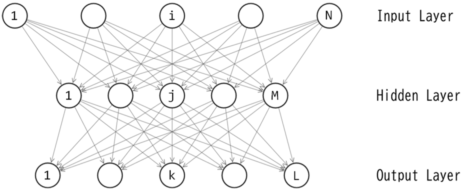
A three-layered perceptron, as depicted in Figure 2, includes M+L unit biases and NM+ML connection weights, resulting in a total of M+L+NM+ML parameters. Let D represent the quantity M+L+NM+ML. For this study, the author sets N=3 and L=1, leading to D=5M+1. The training of this perceptron is essentially an optimization of the D-dimensional binary vector. Let

x = (x_{1}, x_{2}, \dots, x_{D})

denote the D-dimensional vector, where each

x_{i}

corresponds to one of the D parameters in the perceptron. In this study, each

x_{i}

is a binary variable, e.g.

x_{i} \in

{-1,1} or

x_{i} \in

{0,1}. By applying the value of each element in

x

to its corresponding connection weight or unit bias, the feedforward calculations can be processed.

In this study, the binary vector

x

is optimized using Evolution Strategy [10,11,12]. ES treats

x

as a chromosome (a genotype vector) and applies evolutionary operators to manipulate it. The fitness of

x

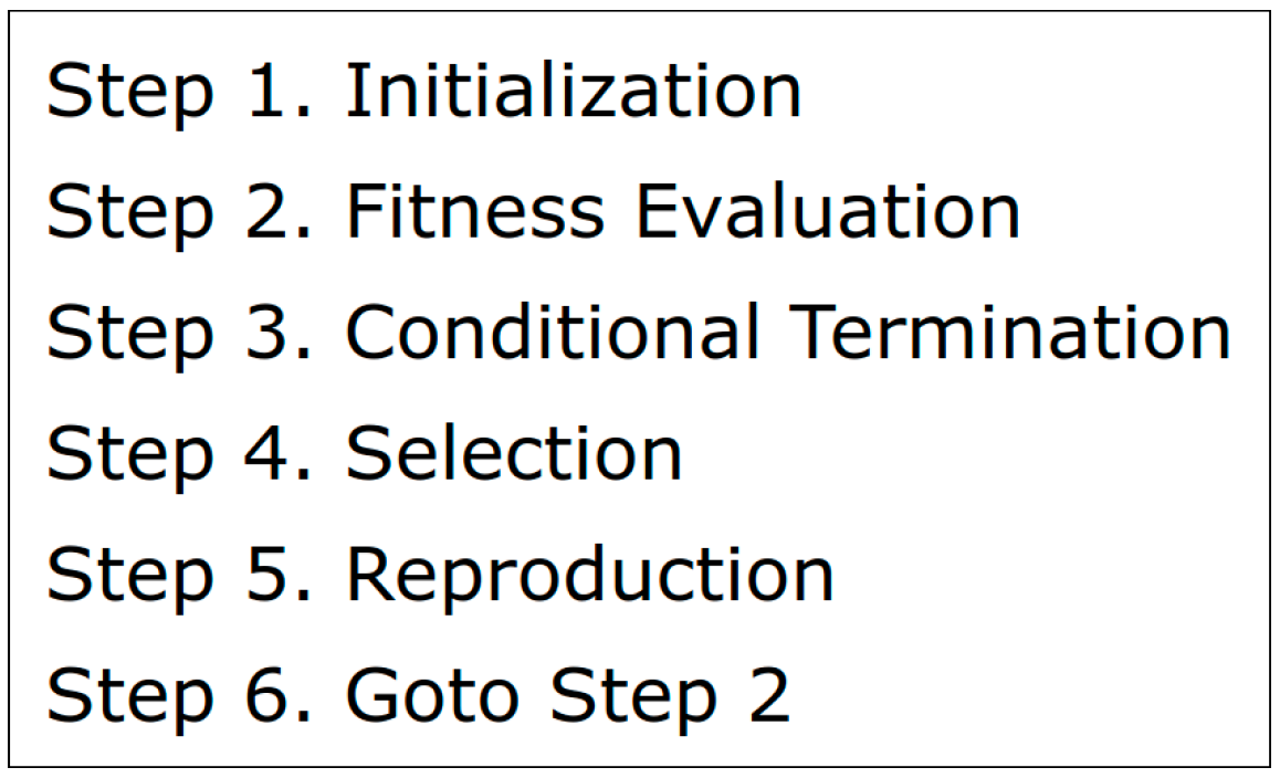
is evaluated based on eq. (1) described in the previous article [1]. Figure 3 illustrates the ES process. The process is the same as that in the previous study [1]. In Step 1, D-dimensional binary vectors

y^{1}, y^{2}, \dots, y^{C}

are randomly initialized where

C

denotes the number of offsprings. A larger value of

C

promotes explorative search more. In Step 2, values in each vector

y^{c}

(

c = 1,2, \dots, C

) are applied to the MLP and the MLP controls the pendulum for a single episode with 200 time steps. The fitness of

y^{c}

is then evaluated with the result of the episode. Let

f (y^{c})

denote the fitness. In Step 3, the loop of evolutionary training is finished if a preset condition is satisfied. A simple example of the condition is the limit number of fitness evaluations. In Step 4, among the

P + C

vectors in the parent population (

z^{1}, z^{2}, \dots, z^{P}

) and the offspring population (

y^{1}, y^{2}, \dots, y^{C}

), vectors with the top

P

fitness scores survive as the parents in the next reproduction, and the remaining vectors are deleted.

P

denotes the number of parents. A smaller value of

P

promotes exploitive search more. Note that, for the first time of Step 4, the parent population is empty so that vectors with the top

P

fitness scores survive among the

C

vectors in the offspring population (

y^{1}, y^{2}, \dots, y^{C}

). In Step 5, new

C

offspring vectors are produced by applying the reproduction operator to the parent vectors (

z^{1}, z^{2}, \dots, z^{P}

) which are selected in the last Step 4. The new offspring vectors form the new offspring population (

y^{1}, y^{2}, \dots, y^{C}

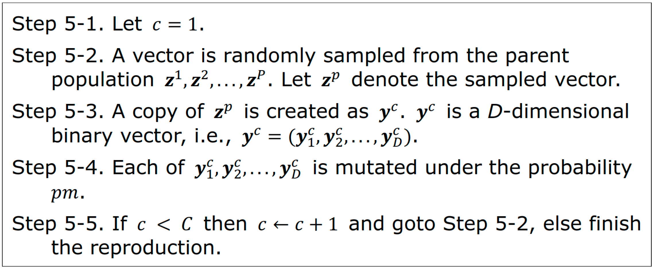
). Figure 4 denotes the process of reproduction. This reproduction process is slightly different from that in the previous study [1] because the genotype vectors are not real-valued vectors but binary ones. In Step5-4, each of

y_{1}^{c}, y_{2}^{c}, \dots, y_{D}^{c}

is mutated under the probability

p m

. Let denote b_S (b_G) is the smaller (greater) value for the binary parameter, e.g. { b_S, b_G } = {-1, 1}. The mutation flips the value of

y_{d}^{c}

from b_S to b_G (or from b_G to b_S). A greater value of

p m

promotes explorative search more.

5. Experiment

In the previous study using MLPs with real-valued connection weights, the number of fitness evaluations included in a single run was set to 5,000 [1]. The number of new offsprings generated per generation was either of (a)

C

=10 and (b)

C

=50. The number of generations for each case of (a) or (b) was 500 and 100 respectively. The total number of fitness evaluations were 10 × 500 = 5,000 for (a) and 50 × 100 = 5,000 for (b). The experiments in this study, using MLPs with binary connection weights, employs the same configurations. The hyperparameter configurations for ES are shown in Table 1. The number of parents, denoted as

P

, is set to 10% of the

C

offsprings for both (a) and (b). The mutation probability

p m

is set to 0.05. The values of

P

and

p m

were adjusted based on preliminary experiments.

Sets of two values such as {-1,1} or {0,1} can be used for the binary connection weights. The author first presents experimental results using {-1,1}. In the previous study using real-valued MLPs, it was found that, among 8, 16, or 32 hidden units, 16 units yielded the most desirable results [1]. The binary MLPs used in this study are expected to require a greater number of hidden units to achieve performance comparable to the real-valued MLP with 16 hidden units. Therefore, in this experiment, the author tested three options: 16, 32, and 64. A binary MLP with either of 16, 32, or 64 hidden units underwent independent training 11 times.

Table 2 presents the best, worst, average, and median fitness scores of the trained MLPs across the 11 runs. Each of the two hyperparameter configurations (a) and (b) in Table 1 was applied. A larger value is better in Table 2 with a maximum of 1.0.

In order to investigate which of the two configurations (a) or (b) is superior, the Wilcoxon signed-rank test was applied to the 12

\times

2 data points presented in Table 2. This test revealed that there was no statistically significant difference between (a) and (b) (p > .05); however, the p-value suggested that configuration (a) is slightly superior to configuration (b). In other words, it was found that reducing the population size and increasing the number of generations is slightly more favorable than the opposite approach. This finding contradicts the result of the previous study [1] where it was observed that, using real-valued MLPs, the configuration (b) was superior to the configuration (a). The cause of this difference will be the variation in the model size of the MLP. In the prior study using real-valued MLPs, the number of hidden units M was either 8, 16, or 32, so that number of parameters D was 41, 81, and 161 respectively (D=5M+1). On the other hand, for the binary MLPs in this study, M was either 16, 32, or 64, so that D was 81, 161, and 321 respectively. As the number D corresponds to the genotype length in ES, a larger D implies longer genotype vectors that ES needs to optimize. In other words, compared to the real-valued MLP in the prior study, the binary MLP in this study requires optimization of longer genotype vectors by ES. To optimize longer genotype vectors more effectively, the configuration (b) which promotes late-stage local exploitation was more suitable in this experiment, as it provided a higher frequency of fine-tuning genetic adjustments.

Next, the author examines whether there is a statistically significant difference in the performances among the three MLPs with the different numbers of hidden units M. For each M of 16, 32, and 64, the author conducted 11 runs using the configuration (a), resulting in 11 fitness scores. The Wilcoxon rank sum test was applied to the 11

\times

3 data points. The results showed that there was little difference between M=64 and M=32 (p = 0.50). While there was no significant difference between M=16 and either M=32 or M=64 (with p-values of 0.067 and 0.058, respectively), the proximity of the p-values to 0.05 indicated that M=16 significantly underperformed compared to both of M=32 and M=64. In other words, M=32 exhibited significantly superior performance to M=16 and little difference to M=64. Therefore, from the perspective of the trade-off between performance and memory size, the most desirable number of hidden units was found to be 32.

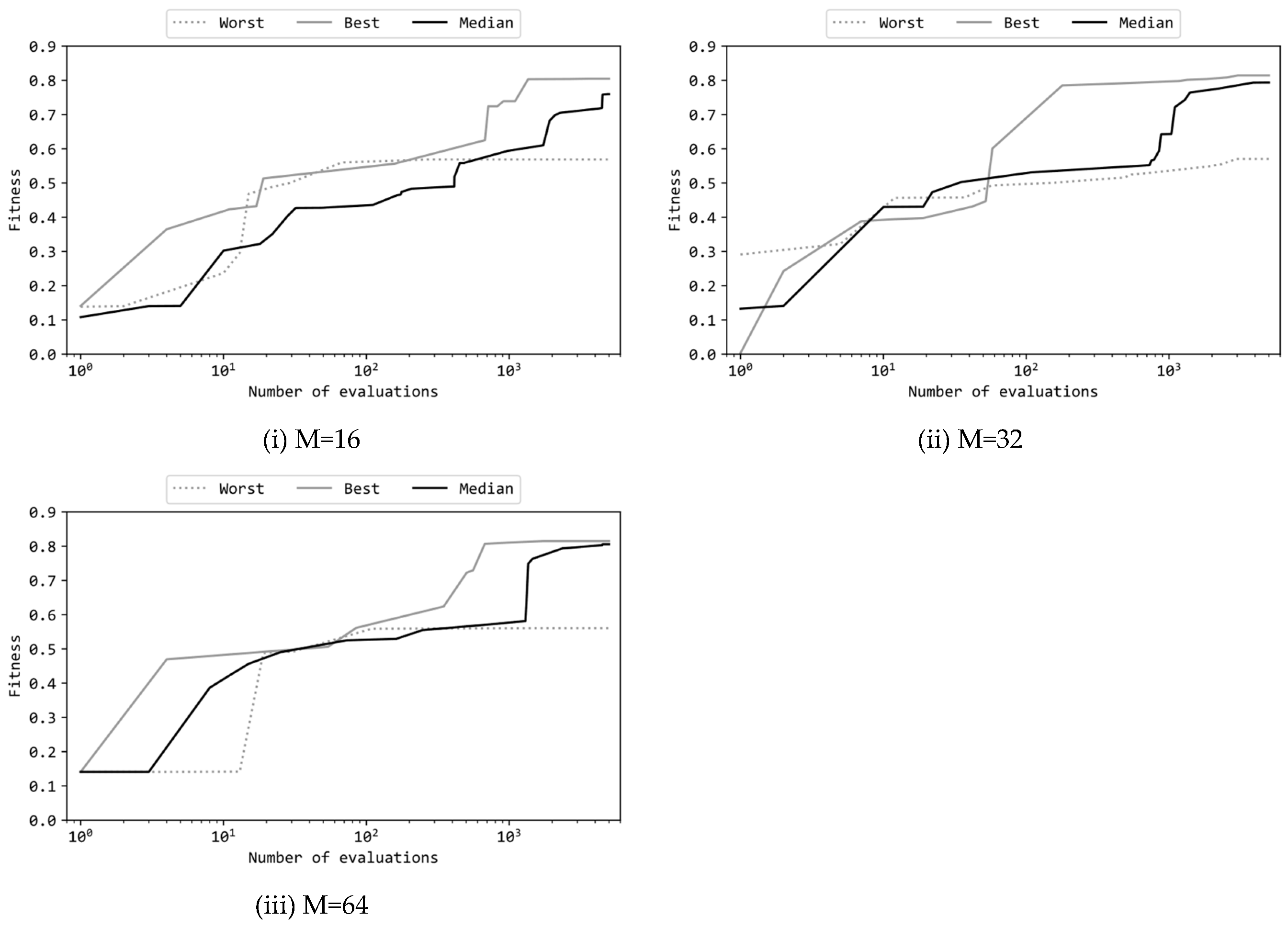
Figure 5 presents learning curves of the best, median, and worst runs among the 11 runs where the configuration (a) was applied. Note that the horizontal axis of these graphs is in a logarithmic scale. Figure 4(i), (ii), and (iii) depict learning curves of MLPs with different numbers of hidden units (M=16, 32, 64). Despite the varying number of hidden units, the curves in Figure 4(i), (ii), and (iii) exhibit similar shapes. Each curve started around a fitness value of 0.1 and rose to approximately 0.5 within the first 10 to 100 evaluations. Given that ES with the configuration (a) produces 10 offsprings per generation, {10, 20, …, 100} evaluations correspond to {1, 2, …, 10} generations. Thus, the learning curves revealed that it was relatively easy for ES to raise the fitness value from 0.1 to 0.5 within the early stage. Subsequently, over the remaining approximately 4900 evaluations (roughly 490 generations), the fitness values increased from around 0.5 to around 0.8. However, in all cases (i), (ii), and (iii), the worst runs did not show an increase in fitness from around 0.5, indicating a failure to achieve the task. On the other hand, the median runs in (i), (ii), and (iii) consistently achieved fitness scores comparable to the best runs, indicating that, at least half of the 11 runs, ES could train the MLPs successfully. Furthermore, the shapes of these learning curves closely resemble those observed when using real-valued MLPs [1], suggesting that, even with binary MLPs, as long as the model size is appropriate, the learning process by ES evolves similarly to that of real-valued MLPs.

In Figure 5(ii), it is noteworthy that the curve of the best run starts around fitness 0.0, while the curve of the worst run starts around fitness 0.3. Both differ from the other graphs, but this discrepancy is attributed to the random variance in the initialization. Of particular interest is that the run starting with lower fitness scores eventually become the best run, while, conversely, the run starting with higher fitness scores end up as the worst run. This suggests that the initial fitness scores being greater does not necessarily result in a greater final fitness score. The reason for this phenomenon is likely that greater initial fitness scores suppress early-stage global exploration due to the mechanism of selection, making it more likely to get trapped in undesirable local optima.

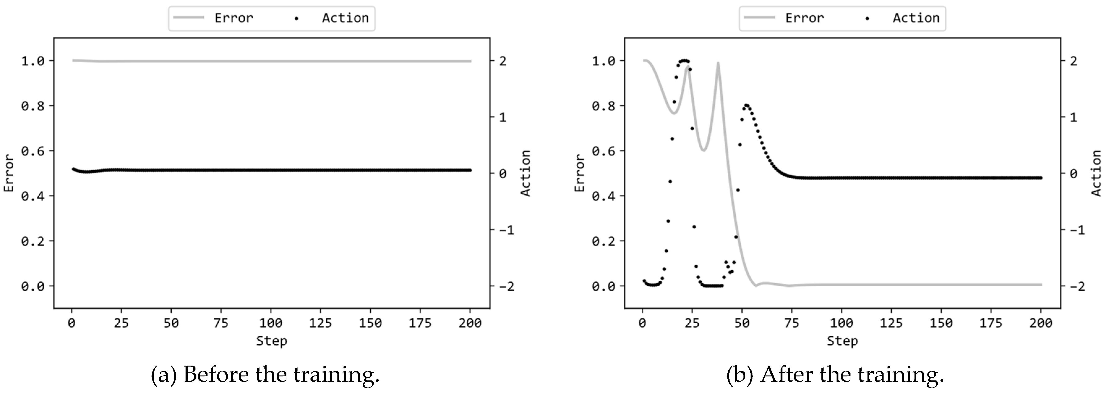
Figure 6(a) illustrates the actions by the MLP and the errors of the pendulum to the target state (values of Error(t) defined in the previous article [1]) in the 200 steps prior to training, while Figure 6(b) displays the corresponding actions and errors after training. In this scenario, the MLP included 16 hidden units, and ES utilized the configuration (a) in Table 1. Supplementary videos are provided which demonstrate the motions of the pendulum controlled by the MLPs before/after trained2^,3. Figure 6(a) reveals that the MLP, right after the random initialization of connection weights (prior to the training), was unable to control the pendulum and thus failed the task. From time t=0 to t=200, it consistently produced almost zero torque output. As a result, the pendulum remained stationary, starting from the initial state where it hanged directly downward (with an error of the maximum value of 1.0 from the target state). On the other hand, Figure 6(b) reveals that the MLP, after the training, could substantially reduce the error to almost zero, indicating successful completion of the task. From time t=0 to around t=40, the torque values fluctuate between the minimum value of -2.0 and the maximum value of 2.0, indicating a swinging motion of the pendulum from side to side. This swinging motion is necessary to lift the pendulum to the upright position; continuously applying torque of -2.0 or 2.0 to the pendulum initially facing downward cannot lift it beyond a certain height. Despite not explicitly instructing the need for this swinging motion, ES successfully trained the MLP to induce the pendulum to swing.

Furthermore, after the error approached zero around time t=75, the torque output from the MLP also approached zero. This observation indicates that the MLP maintained the inverted position without providing unnecessary torque to the balanced pendulum. Since a more extended duration of the pendulum remaining in an inverted state leads to a higher fitness score, it is desirable to bring the pendulum into the upright position as quickly as possible. From the error curve in Figure 6(b), it is evident that the pendulum swung for only two cycles initially and then promptly achieved an inverted position. In other words, ES effectively manipulated the genotype vectors to maximize the fitness scores, demonstrating the discovery of sufficiently good solutions that rapidly bring the pendulum to the target state.

As reported above, among 16, 32, and 64, 32 was the best number of hidden units in the binary MLP. The binary MLP with 32 hidden units includes 161 parameters (D=5M+1=161) so that the MLP requires 161 bits to store in memory. On the other hand, the prior article [1] reported that, among 8, 16, and 32, 16 was the best number of hidden units in the real-valued MLP. In both studies, the same training algorithm (ES) and the same pendulum task were adopted. A real-valued MLP with 16 hidden units includes 81 parameters (D=5M+1=81) so that the MLP requires 2,592 or 5,184 bits to store, using 32 bits or 64 bits per floating-point number respectively. To compare the performance of the binary MLP with 32 hidden units and the real-valued MLP with 16 hidden units, the Wilcoxon rank sum test was applied to the data of fitness scores obtained by the MLPs. Although the real-valued MLP with 16 hidden units exhibited better fitness scores, the difference was not statistically significant (p = .086). In terms of memory size, the binary MLP with 16 hidden units can be stored using only 6.2% (161 bits/2,592 bits) or 3.1% (161 bits/5,184 bits) of the memory required by real-valued MLPs with 32 hidden units. After the training, the binary MLP efficiently inverted the pendulum and maintained this state, similarly to the real-valued MLP. Thus, binary MLPs are useful from the perspectives of task performance and memory size, and ES demonstrated its ability to the reinforcement training of binary MLPs under appropriate configurations.

The above in this article reported the experimental result where {-1,1} were used as the binary values for the connection weights. The author next presents the experimental result using {0,1} instead of {-1,1}. A connection with a weight of 0 is equivalent to be disconnected, signifying its redundancy. Therefore, the presence of numerous connections with the weight of 0 implies a lighter feedforward computation for the neural network.

Table 3 presents the best, worst, average, and median fitness scores of the trained MLPs across the 11 runs. Based on the results with {-1,1}, the number of hidden units in the MLP was set to 32 and the ES utilized the configuration (a) in Table 1. Comparing Table 3 with Table 2 reveals that the values in Table 3 are consistently smaller than their corresponding values in Table 2. Thus, the performance of MLPs with {0,1} weights were inferior to those with {-1,1} weights. The Wilcoxon rank sum test to the 11 fitness scores for each case reveals that this difference is statistically significant (p < .01).

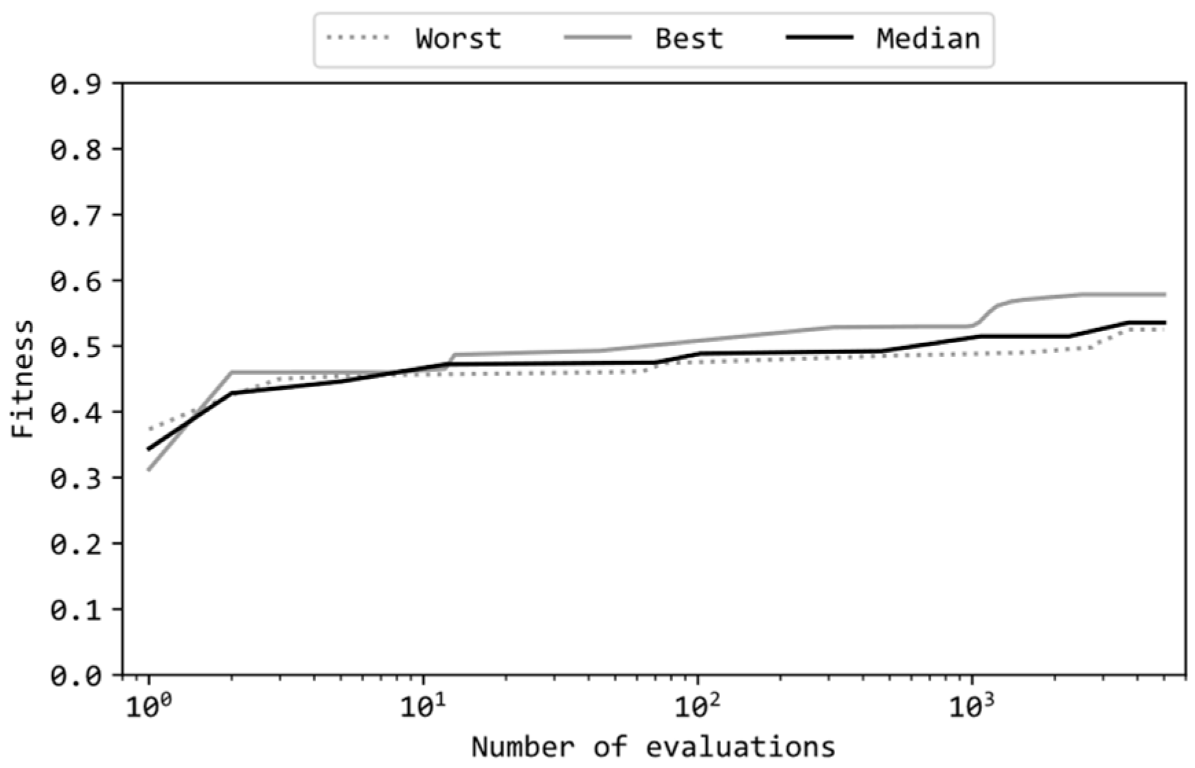
Figure 7 illustrates the learning curves of the MLP with {0,1} weights in the same format as Figure 5. The shapes of the curves in Figure 7 are clearly different from those in Figure 4(ii). Figure 7 reveals that the learning curves of {0,1} MLPs for the best, median, and worst runs among the 11 runs closely resemble each other, all commencing around a fitness score of 0.3 and concluding near 0.5. In contrast, Figure 4(ii) shows that the learning curves of the {-1,1} MLPs for both the best and median runs progressed up to around 0.8.

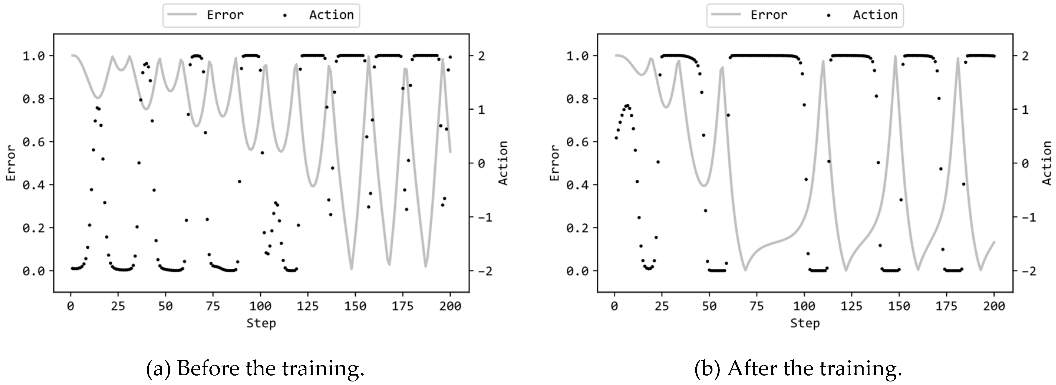
Figure 8 illustrate the actions by the {0,1} MLPs and the errors of the pendulum to the target state, in the same format as Figure 6. The MLP included 32 hidden units, and ES utilized the configuration (a) in Table 1. The graphs are significantly different between the cases of {0,1} (Figure 8) and {-1,1} (Figure 5) for both (a) untrained and (b) trained. Supplementary videos are provided which demonstrate the motions of the pendulum controlled by the {0,1} MLPs before/after trained 4^,5. The {0,1} MLP before the training exhibited a behavior where, despite random initialization of connection weights to either 0 or 1, it first swung the pendulum and then rotated it. This behavior can be attributed to the fact that the absence of negative values in the connection weights: the input values to the units in the hidden and output layers are more likely to be positive (or negative) when the input values to the units in the input layer are positive (or negative). This results in torque applied to the pendulum that tends to be close to the maximum value of 2.0 or the minimum value of -2.0. Furthermore, the trained {0,1} MLP, while rotating the pendulum at an earlier stage compared to the untrained {0,1} MLP, failed to stabilize the pendulum in an inverted position as shown by the trained {-1,1} MLP. Similar to the untrained {0,1} MLP, the trained {0,1} MLP repetitively output torque values close to the maximum value of 2.0 or the minimum value of -2.0.

Based on the aforementioned observations, it is evident that employing {0,1} as the connection weights for binary MLP is not appropriate and the use of {-1,1} is superior.

6. Conclusion

In this study, Evolution Strategy was applied to the reinforcement learning of a neural network controller for the pendulum task, where the connection weights in the neural network are not real numbers but binary. The experimental result was compared with another result of the previous experiment [1] in which the connection weights were real numbers. The findings from this study are summarized as follows:

(1): The optimal number of hidden units for the binary MLP was found to be 32 among the choices of 16, 32, and 64.
(2): The configuration (a) yielded superior results compared to the configuration (b) in Table 1. The configuration (a) involved a smaller population size and a larger number of generations compared to the configuration (b).
(3): The binary MLP with 32 hidden units performed worse than the real-valued MLP with 16 hidden units, but the difference between their performances was not statistically significant (p > .05).
(4): The motion of the pendulum controlled by the binary MLP after the training showed that the binary MLP successfully swung the pendulum swiftly into an inverted position and maintained its stability after inversion, as the real-valued MLP had done. Thus, ES demonstrated effective reinforcement learning capabilities for both real-valued and binary MLPs.
(5): The memory size required to record the binary MLP with 32 hidden units is 3.1% or 6.2% of the memory size required to record a real-valued MLP with 16 hidden units. From the perspectives of task performance and memory size, it was confirmed effective to binarize connection weights.
(6): As the values of binary weights, {-1, 1} were significantly superior to {0, 1} (p < .01).

The author plans to further apply and evaluate another evolutionary algorithms to the same task and compare the performance.

Acknowledgments

The author conducted this study under the Official Researcher Program of Kyoto Sangyo University.

References

Okada, H. (2022). Evolutionary reinforcement learning of neural network controller for pendulum task by evolution strategy. International Journal of Scientific Research in Computer Science and Engineering, 10(3), 13–18.
Courbariaux, M., Bengio, Y., & David, J.P. (2015). BinaryConnect: training deep neural networks with binary weights during propagations. Proceedings of the 28th International Conference on Neural Information Processing Systems (NIPS’15), 2, MIT Press, 3123–3131. [CrossRef]
Courbariaux, M., Hubara, I., Soudry, D., El-Yaniv, R., & Bengio, Y. (2016). Binarized neural networks: Training deep neural networks with weights and activations constrained to +1 or -1. arXiv preprint arXiv:1602.02830. [CrossRef]
Tang, W., Hua, G., & Wang, L. (2017). How to train a compact binary neural network with high accuracy?. Proceedings of the AAAI Conference on Artificial Intelligence, 31(1). [CrossRef]
Lin, X., Zhao, C., & Pan, W. (2017). Towards accurate binary convolutional neural network. Proceedings of the 31st International Conference on Neural Information Processing Systems (NIPS’17), 344–352. [CrossRef]
Bethge, J., Yang, H., Bartz, C., & Meinel, C. (2018). Learning to train a binary neural network. arXiv preprint arXiv:1809.10463. [CrossRef]
Qin, H., Gong, R., Liu, X., Bai, X., Song, J., & Sebe, N. (2020). Binary neural networks: a survey. Pattern Recognition, 105, 107281. [CrossRef]
Yuan, C., & Agaian, S.S. (2023). A comprehensive review of binary neural network. Artificial Intelligence Review, 56, 12949–13013. [CrossRef]
Sayed, R., Azmi, H., Shawkey, H., Khalil, A. H., & Refky, M. (2023). A systematic literature review on binary neural networks. IEEE Access, 11, 27546–27578. [CrossRef]
Schwefel, H.P. (1984). Evolution strategies: A family of non-linear optimization techniques based on Imitating some principles of organic evolution. Annals of Operations Research, 1, 165–167. [CrossRef]
Schwefel, H.P. (1995). Evolution and Optimum Seeking. Wiley & Sons.
Beyer, H.G., & Schwefel, H.P. (2002). Evolution strategies: A comprehensive introduction. Journal Natural Computing, 1(1), 3–52. [CrossRef]

Figure 1. Pendulum system1.

Figure 2. Topology of the MLP.

Figure 3. Process of evolution strategy.

Figure 4. Reproduction process in evolution strategy.

Figure 5. Learning curves of MLP with M hidden units.

Figure 6. MLP actions and errors in an episode.

Figure 7. Learning curves of MLP with 32 hidden units and {0,1} weights.

Figure 8. MLP actions and errors in an episode ({0,1} weights).

Table 1. ES Hyperparameter Configurations.

Hyperparameters	(a)	(b)
Number of offsprings ( $C$ )	10	50
Generations	500	100
Fitness evaluations	10 $\times$ 500=5,000	50 $\times$ 100=5,000
Number of parents ( $P$ )	10 $\times$ 0.1=1	50 $\times$ 0.1=5
Mutation probability ( $p m$ )	0.05	0.05

Table 2. Fitness Scores among 11 Runs.

	M	Best	Worst	Average	Median
(a)	16	0.805	0.569	0.713	0.760
	32	0.814	0.570	0.757	0.794
	64	0.815	0.561	0.733	0.806
(b)	16	0.789	0.566	0.607	0.570
	32	0.814	0.597	0.748	0.795
	64	0.816	0.591	0.752	0.806

Table 3. Fitness Scores among 11 Runs ({0,1} Weights).

	M	Best	Worst	Average	Median
(a)	32	0.578	0.525	0.539	0.536

Notes

1.	https://www.gymlibrary.dev/environments/classic_control/pendulum/
2.	https://youtu.be/nJ3ni05BdRg
3.	https://youtu.be/-IOF4RcIxZ4
4.	https://youtu.be/JBZBLBIvIrg
5.	https://youtu.be/BHqBj5kthxU

Disclaimer/Publisher’s Note: The statements, opinions and data contained in all publications are solely those of the individual author(s) and contributor(s) and not of MDPI and/or the editor(s). MDPI and/or the editor(s) disclaim responsibility for any injury to people or property resulting from any ideas, methods, instructions or products referred to in the content.

© 2023 by the authors. Licensee MDPI, Basel, Switzerland. This article is an open access article distributed under the terms and conditions of the Creative Commons Attribution (CC BY) license (http://creativecommons.org/licenses/by/4.0/).

Copyright: This open access article is published under a Creative Commons CC BY 4.0 license, which permit the free download, distribution, and reuse, provided that the author and preprint are cited in any reuse.

MDPI Initiatives

Important Links

Choose an area of interest and we will send you notifications of new preprints at your preferred frequency.

Disclaimer