Preprint
Article

Proof of the Riemann Hypothesis Using the Decomposition Zeta(s) = X(s) – Y(s)

Altmetrics

Downloads

145

Views

67

Comments

0

This version is not peer-reviewed

Submitted:

20 December 2023

Posted:

21 December 2023

You are already at the latest version

Alerts
Abstract
Prime numbers are the atoms of mathematics and mathematics is needed to make sense of the real world. Finding the Prime number structure and eventually being able to crack their code is the ultimate goal in what is called Number Theory. From the evolution of species to cryptography, Nature finds help in Prime numbers. One of the most important advances in the study of Prime numbers was the paper by Bernhard Riemann in November 1859 called “Ueber die Anzahl der Primzahlen unter einer gegebenen Grösse” (On the number of primes less than a given quantity). In that paper, Riemann gave a formula for the number of primes less than x in terms the integral of 1/log(x) and the roots (zeros) of the zeta function defined by: Where ζ(z) is a function of a complex variable z that analytically continues the Dirichlet series. Riemann also formulated a conjecture about the location of the zeros of RZF, which fall into two classes: the "trivial zeros" -2, -4, -6, etc., and those whose real part lies between 0 and 1. Riemann's conjecture Riemann hypothesis [RH] was formulated as this: [RH] The real part of every nontrivial zero z* of the RZF is 1/2. Proving the RH is, as of today, one of the most important problems in mathematics. In this paper we will provide a proof of the RH. The proof of the RH will be built following these five parts: PART 1: Description of the RZF PART 2: The C-transformation PART 3: Application of the C-transformation to in Re(z) 0 to obtain ζ(z)=X(z)-Y(z) PART 4: Analysis of the values of z such that X(z)=Y(z), and |X(z)|=|Y(z)|, that equates to ζ(z)=0 Proof that |X(z)|=|Y(z)| only if Re(z)=1/2 Conclude that ζ(z)=0 only if Re(z)=1/2 for Re(z) 0 PART 5: We will also prove that all non-trivial zeros of ζ(z) in the critical line of the form are not distributed randomly. There is a relationship between the values of those zeros and the Harmonic function that leads to an algebraic relationship between any two zeros.
Keywords: 
Subject: Computer Science and Mathematics  -   Algebra and Number Theory

PART 1: The Riemann Zeta function ζ( s ) [RZF]

1.
ζ ( s )   i n   R  
As defined in literature (Sondow et al, Weisstein, Edwards, Jekel)
1.1.
ζ s = j = 1 j s   c o n v e r g e s   f o r   s 1
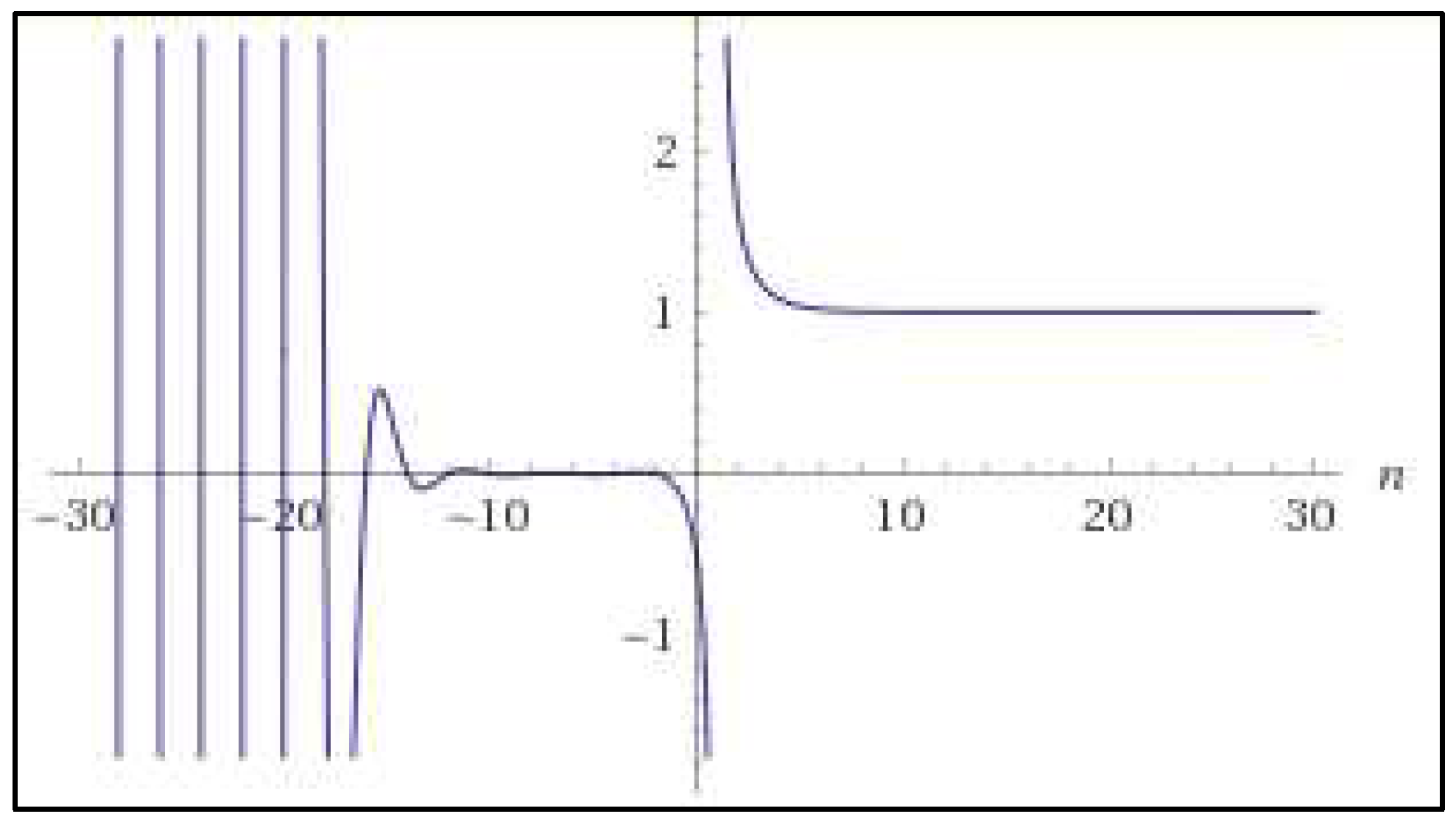
Figure 1. Riemann Zeta function in R.
Preprints 93993 g001
  • 1.2.
    Euler Product Formula that links ζ s with the distribution of prime numbers
    ζ s = j = 1 j s = p = p r i m e 1 1 p s
    Example for k=2
    1 1 2 + 1 2 2 + 1 3 2 + 1 4 2 + = 1 1 2 2 x   1 1 3 2 x 1 1 5 2 x 1 1 7 2 x
    1.3.
    Integral definition of ζ s :
    ζ s = j = 1 j s = 1 Γ ( s ) 0 1 e x 1 x s d x x
    Where Γ ( s ) , is the Gamma function
    1.4.
    Analytical continuation of ζ s for :
    Re(s)>0: [Dirichlet]
    ζ s = 1 s 1 k = 1 ( n n + 1 s n s n s
    0<Re(s)<1:
    ζ s =   1 1 2 1 s k = 1 1 k 1 k s
    -k<Re(s) [Kopp, Konrad. 1945]:
    ζ s =   1 s 1 k = 1 k ( k + 1 ) 2 ( 2 k + 3 + s ) ( k + 1 ) s + 2 2 k 1 s k s + 2 )
    1.5.
    Laurent series of ζ s :
    ζ s =   1 s 1 + k = 1 k γ n k ! s 1 k )
    where γ n are the Stieltjes constants.
    1.6.
    Hurwitz function ζ k , z :
    ζ k , z = j = 0 j + z k = j = z j k   c o n v e r g e s   f o r   k > 1
    1.7.
    Generalized Harmonic Function H n k :
    H n k = j = 1 n j k = 1 1 k + 1 2 k + + 1 n k             c o n v e r g e s   f o r   k > 1
    1.8.
    ζ(s) converges for s>1 to the following values (Sloane):
    Table 1. Values of ζ(s).
    Table 1. Values of ζ(s).
    s ζ(s) Known ζ(s) representations over π
    2 1.6449179 π2/6
    4 1.0823232 π4/90
    6 1.0173431 π6/945
    8 1.0040774 π8/9450
    1.9.
    An approximation for the values of ζ s for s>1 in R
    One can calculate that:
    lim ( s ζ s ζ s + 1 ) 1 s = 1
    And:
    lim s ( ζ s ζ s 1 ) 1 s = 2
    Based on this expression, for s sufficiently large, one can represent ζ s   as a multiple of π s :
    ζ s = π s K s   with   K s   =   2 s 1 π s 2 s
    with a very good approximation given by:
    K s   =   i n t 2 s 1 π s 2 s 1               with   int ( k )   is   the   integer   part   of   k .
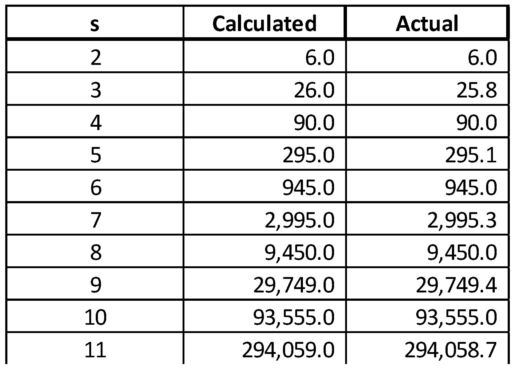
    The error between the K s calculated and K s actual is very small for s>4.
    Some calculated values of K s calculated and K s actual:
    Table 2. Values of K s calculated and K s actual.
    Table 2. Values of K s calculated and K s actual.
    Preprints 93993 i001
    One can use [2] to propose the following approximation for ζ s :
    C Z s = 1 1 π s 2 s
    Table 3. Comparing ζ s and CZ(s).
    Table 3. Comparing ζ s and CZ(s).
    s=3 s=4 s=10 s=14
    ζ s 1.20206 1.0823 1.000994 1.0000612
    C Z s 1.18659 1.0784 1.000988 1.0000611
    Graphically:
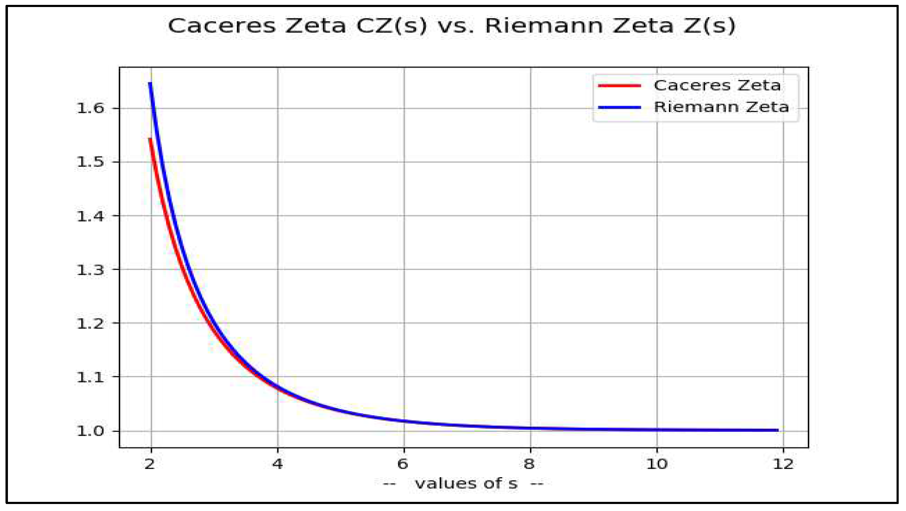
Figure 2. Caceres’ approximation for the Riemann Zeta function in R.
Preprints 93993 g002
  • 1.10.
    Zeros of ζ z (Weisstein)
    1.10.1.
    R e ( z ) > 1
    There are no zeros of ζ s . ζ s converges for s>1.
        1.10.2.
    z = 1
    ζ 1 is the Harmonic function and diverges, and:
    lim s 1 ( ζ s 1 1 s ) =   γ (the Euler-Mascheroni constant)
        1.10.3.
    R e ( z ) < 1
    ζ z has trivial zeros at z = 2 k , with k natural numbers
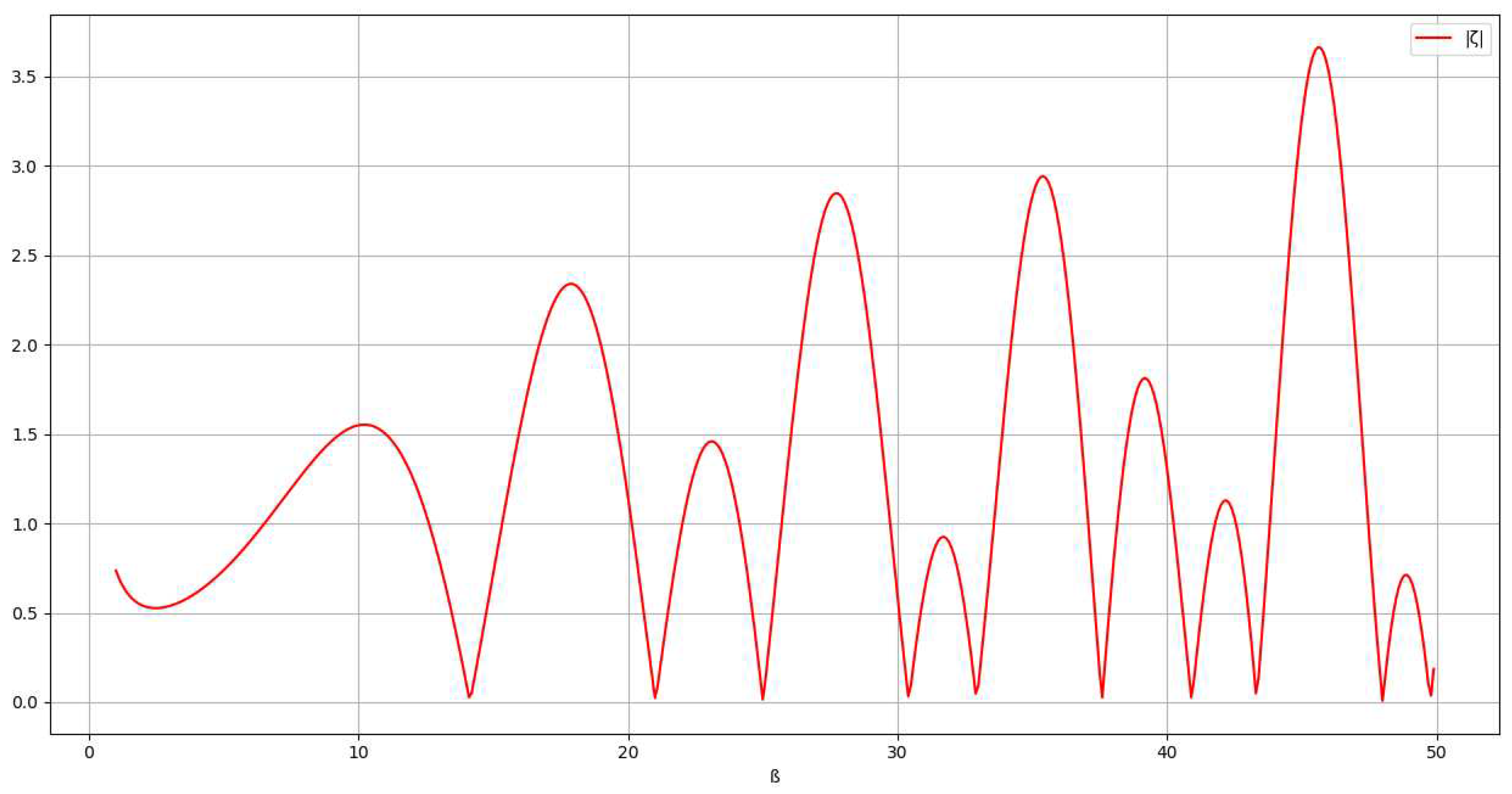
    ζ z has nontrivial zeros at z   = 1 2 ±   ß i at the critical line R e ( z ) = 1 2 (Brentt)
    The Riemann Hypothesis [RH] establishes that all nontrivial zeros of zeta have R e ( z ) = 1 2 List of imaginary part of the first nontrivial zeros of zeta (Odlyzko):
    • ß(1)    = 14.134725142
    • ß(3)    = 25.010857580
    • ß(4)    = 30.424876126
    • ß(6)    = 37.586178159
    • ß(7)    = 40.918719012
    • ß(9)    = 48.005150881
    • ß(10) = 49.773832478
    Representation of | ζ z | :
Figure 3. Modulus of the Riemann Zeta function | ζ z | .
Preprints 93993 g003

PART 2: The C-Transformation

1.
C-Transformation of f(x)
Let’s define the C-transformation of an integrable function f(x) by:
C n f x =   k = 1 n f k   f n   d n
And the C-values is the limit, if it exists, of the C-transformation when n :
C f x = lim n C n f x  
1.1.  C-Transformation of f x = 1 x for x R :
C n 1 x = k = 1 n 1 k d n n
And the C-Value of f x = 1 x is γ = 0.5772 (Euler-Mascheroni constant)
C 1 x = lim n ( k = 1 n 1 k l n ( n ) ) = γ
1.2.  C-Transformation of f x = ln x m x for x R , m Z :
C n ln x m x = k = 1 n ln k m k ln n m d n n
And the C-Value of f x = ln x m x are the Stieltjes constants that occur in the Laurent series expansion of the Riemann zeta function:
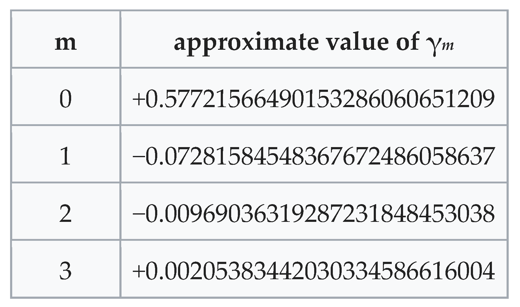
C ln x m x = lim m ( k = 1 m ( ln k ) n k ( ln n ) m + 1 m + 1 ) = γ m
Preprints 93993 i006
1.3.  C-Transformation of f x = m , for m R constant:
C n m = k = 1 n m m   d n
C n m = m n m n = 0
and the C-values of f(x) =m constant is:
C m = 0
1.4.  C-Transformation of f x = sin x for x R :
C n sin x = k = 1 n sin k sin n d n
C n sin x = 1 2 sin n cot 1 2 cos n + cot 1 2 + cos n
And the C-values of f x = sin x are in the interval:
C sin x 1 2 2 cot 1 2 3 ,   3 2
One can also calculate that:
C cos x 1 2 cot 1 2 4 , 1 2 2 cot 1 2
1.5.  C-Transformation of f x = e x for x R :
C n e x = k = 1 n e k e n d n
C n sin x = k = 1 n e k + e n n
And the C-values of f x = e x are:
C e x = 1 e 1
1.6.  C-Transformation of f x = x s for x , s R , s>1:
C n 1 x s = k = 1 n 1 k s d n n s
C n 1 x s = k = 1 n 1 k s n 1 s 1 s
and the C-value of f x = 1 x s is the Riemann Zeta function for s>1:
C 1 x s = lim n ( k = 1 n 1 k s n 1 s 1 s ) = lim n ( k = 1 n 1 k s ) lim n ( n 1 s 1 s ) = ζ ( s )
1.7.  C-Transformation of f z = 1 x z for z C , R e z 0 , z 1
C n 1 x z = k = 1 n 1 k z d n n z
One can use Euler’s identity:
e x = cos x + i sin x
To calculate for z=α+ßi:
k z = k α     [ cos ß ln k i   ( s i n ( ß ln k ) ]
And:
d n n z = n 1 α [ cos ( ß ln n i sin [ ß ln n ]     1 α + i ß [ 1 α 2 + ß 2 ]
One can now express the real and imaginary components of C n f as:
R e ( C n f ) =   k = 1 n k α   ( c o s ( ß ln k )   + +   1 [ 1 α 2 + ß 2 ]   ( n 1 α   [ ( 1 - α ) * cos ( ß * ln ( n ) ) + ß * sin ( ß * ln ( n ) ) ] )
I m C n f =   k = 1 n k α   ( s i n ( ß ln k ) + +   1 [ 1 α 2 + ß 2 ]   ( n 1 α   [ ß * cos ( ß * ln ( n ) )   -   ( 1 - α ) * sin ( ß * ln ( n ) ) ] )
One can calculate that, for α=Re(z)>1, and for any ϵ arbitrarily small, there is a value of n=N such that for n>N, C N f   - ζ( z )< ϵ , as the following table shows:
Table 4. Values of C n f n = k z for α=Re(z)>1 for N=500.
α ß C N f for N=500 ζ ( z ) | C _ N   { f } ζ ( z )|
2 0 1.644934068 1.654934067 < 10 8
2 1 1.150355702 + 0.437530865 i 1.150355703+0.437530866 i < 10 8
3 3 0 1.202056903 1.202056903 < 10 9
That shows that the C-values of f z = 1 x z for Re(z)>1 is ζ z .

PART 3: A decomposition of ζ(z) based on the C-transformation of f x = 1 x z . for z C , 0 R e z < 1

  • C-Transformation of f z = 1 x z for z C , 0 R e z < 1
The C-values of f z = 1 x z from [6] and [7] are equal to the ζ( z ) when Re(z)>1, this error | C n f   - ζ( z )| grows significantly in the critical strip f o r   0 R e ( z ) < 1 as observed in the following table:
Table 5. Values of C n f n = k z for 0 Re(z)<1 for N=500.
A ß C n f ζ ( z ) | C _ n   { f } ζ ( z )|
0.0 0 CN{f} for N=500 -0.5 0.5
0.2 2 0.399824505+0.322650799 i 0.360103 + 0.266246 i > 0.05
0.7 0 -2.777900606 -2.7783884455 > 10 4
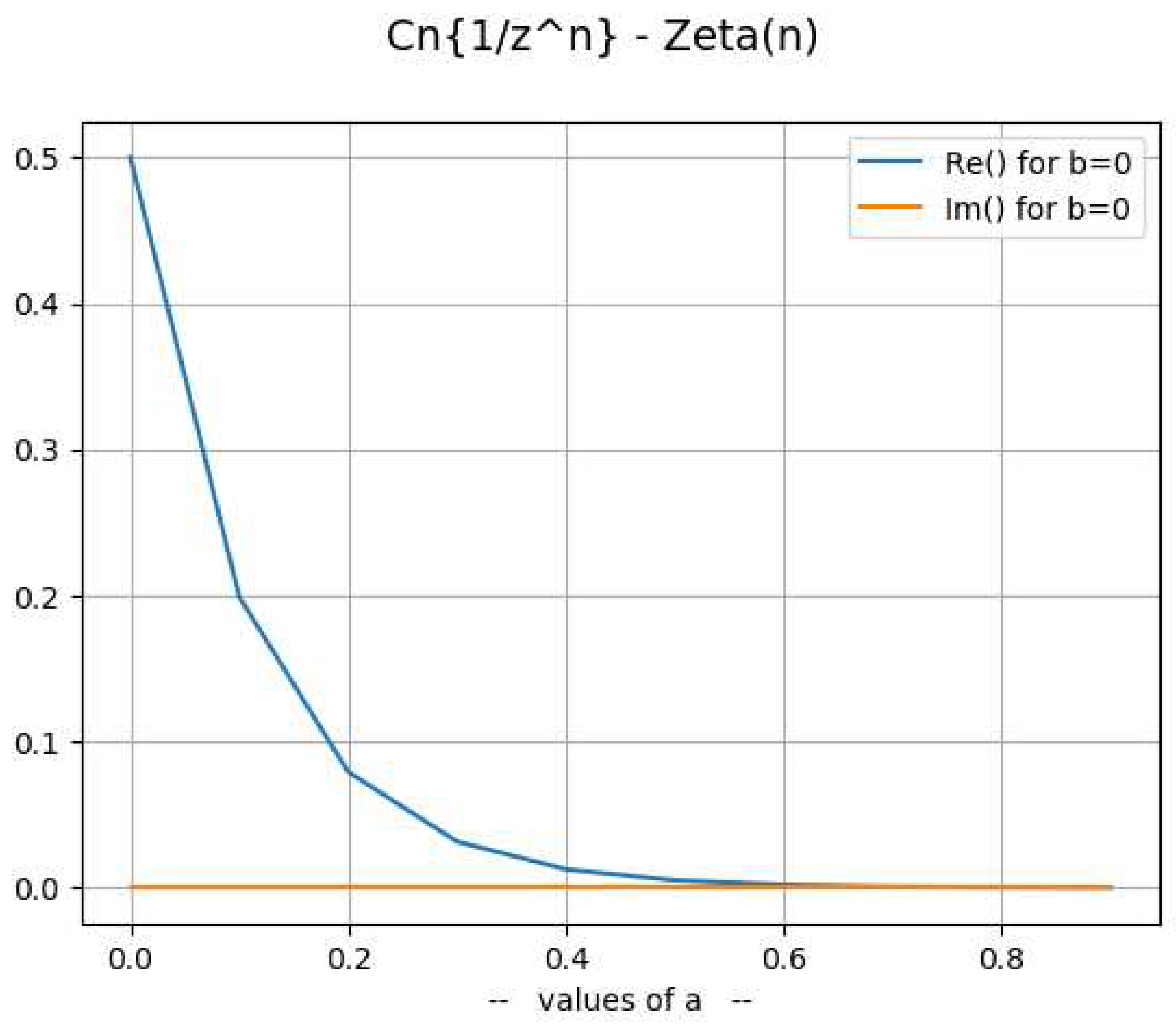
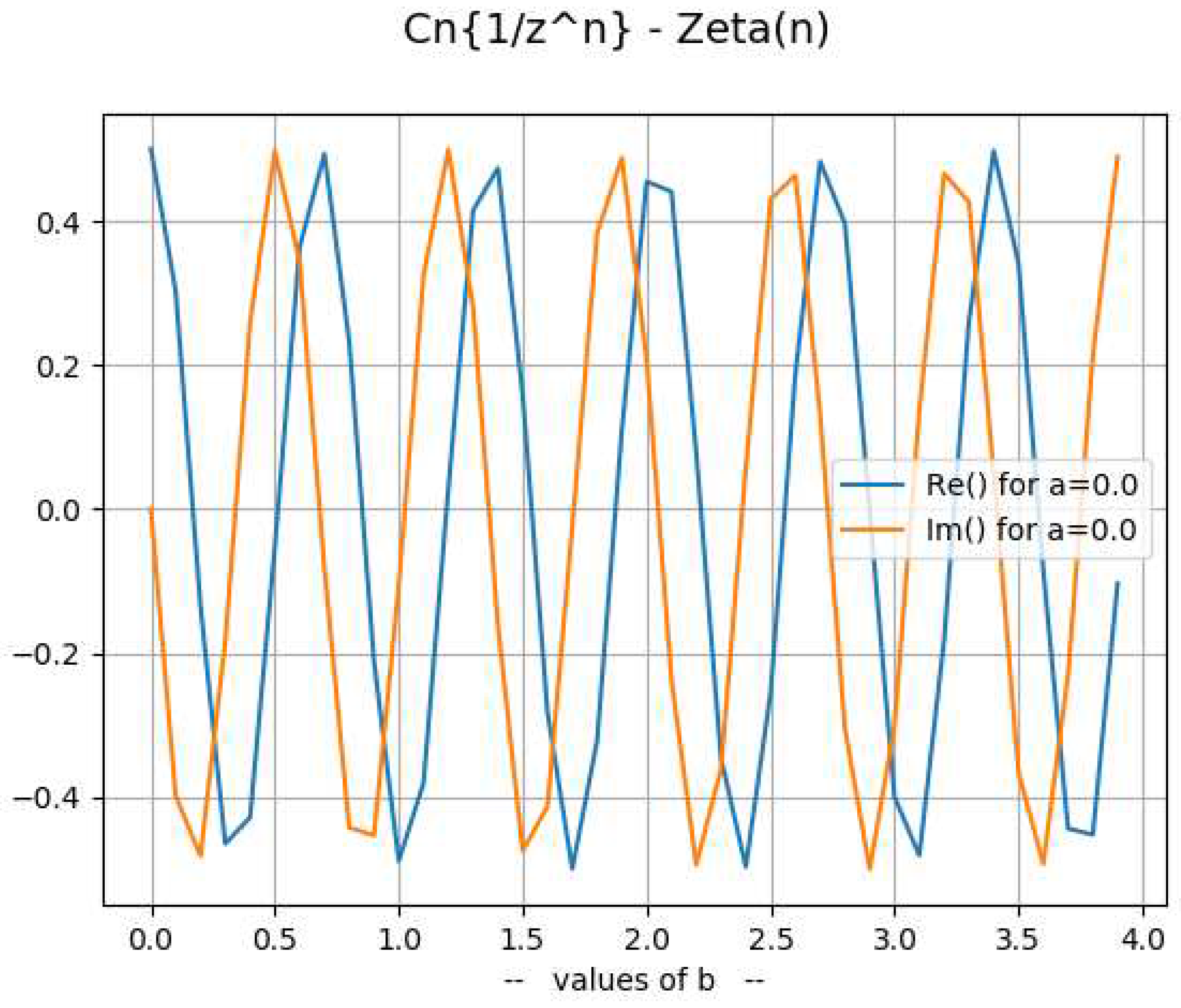
To understand better the value of the difference C n 1 k z   - ζ( z ), one can plot the difference for α 0,1   a n d   ß = 0 : (Similar exponential charts occur for all values of α 0,1 for any given value of ß)
Figure 4a. Where a=Re(z) and b=Im(z).
Preprints 93993 g004a
And plot the difference for variable values of ß 0,1   a n d   α = 0 : (Similar sine charts occur for all values of ß 0,1 for any given value of α)
Figure 4b. Where a=Re(z) and b=Im(z).
Preprints 93993 g004b
These charts lead to the following calculation of the difference C n 1 k z   ζ z :
Re [ C n 1 k z   ζ ( z ) ] = 1 2   n a c o s ( ß l n ( n ) ) + O ( 1 n )
Im [ C n 1 k z ζ ( z ) ] = 1 2   n a s i n ( ß l n ( n ) ) + O ( 1 n )
With O ( 1 / n ) > 0 when n > .
And one can finally write:
R e ( C n f ) =   k = 1 n k α   ( c o s ( ß ln k ) + +   1 [ 1 α 2 + ß 2 ]   ( n 1 α   [ ( 1 - α ) * cos ( ß * ln ( n ) ) + ß * sin ( ß * ln ( n ) ) ] ) + 1 2   n a cos ß ln n
I m C n f = k = 1 n k α   ( s i n ( ß ln k ) + 1 [ 1 α 2 + ß 2 ]   ( n 1 α   [ ß * cos ( ß * ln ( n ) )   -   ( 1 - α ) * sin ( ß * ln ( n ) ) ] ) + 1 2   n a sin ß ln n
and the C-value of f x = 1 x z for z C ,   R e z 0 ,   z 1 is the Riemann Zeta function ζ(z).
2.
Decomposition of ζ z = X z Y z
One can rewrite [8] and [9] creating the X ( z , n ) and Y ( z , n ) functions:
ζ ( z )   =   lim n X z , n   Y z , n , where:
X ( z ,   n )   =   ( k = 1 n k α c o s ( ß ln k ) + 1 2   n α c o s ( ß ln n ) + +   i ( k = 1 n k α s i n ( ß ln k ) + 1 2   n α sin ß ln n ) )
Y ( z ,   n ) = n 1 α 1 [ 1 α 2 + ß 2 ] [ 1 α cos ß ln n + ß sin ß ln n + + i ( ß cos ß ln n 1 α sin ß ln n ) ]
and define:
X z =   lim n X z , n   and
Y z = lim n Y z , n                  
to write:
ζ z = X z Y z
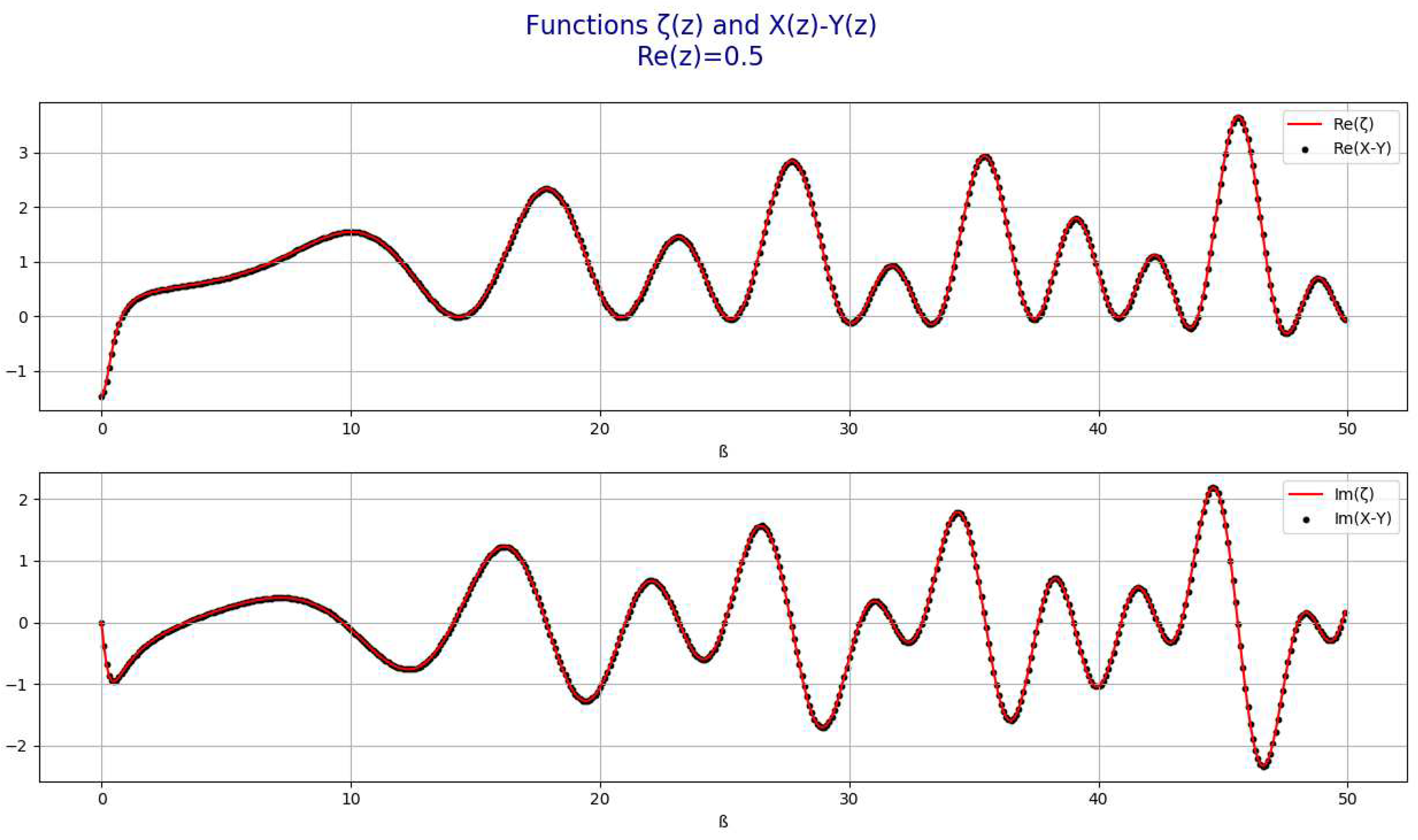
The following table compared the values of ζ z   and X z Y z :
Table 6. ζ(z) compared to X(z) - Y(z).
  z= 0 +j* 0 and n=500
    Zeta(z) = -0.5 + i* 0.0
     X(z)-Y(z) = -0.5 +i* 0.0
     ---> Error = 0.0 +i* 0.0
  z= 0.2 +j* 2 and n=500
      Zeta(z) = 0.360102590022591 + i* -0.266246199765574
      X(z)-Y(z) = 0.360102741838091 +i* -0.266246128959438
      ---> Error= -1.5181550 e-7 +i* -7.080613 e-8
  z= 0.4 +j* 0 and n=500
      Zeta(z) = -1.13479778386698 + i* 0.0
      X(z)-Y(z) = -1.1347977871726 +i* 0.0
      ---> Error= 3.305619 e-9 +i* 0.0
The highest error for α 0,1 ,     ß 0,100 ,   n=1000 is 8 x 10 6 .
3.
Representation of the function ζ z = X ( z ) Y z for Re(z)=1/2
Figure 5. ζ(z) = X(z) - Y(z).
Preprints 93993 g005
4.
Representation of the function | ζ z | = | X ( z ) Y z | for Re(z)=1/2
Figure 6. |ζ(z)| = |X(z) - Y(z)|.
Preprints 93993 g006
5.
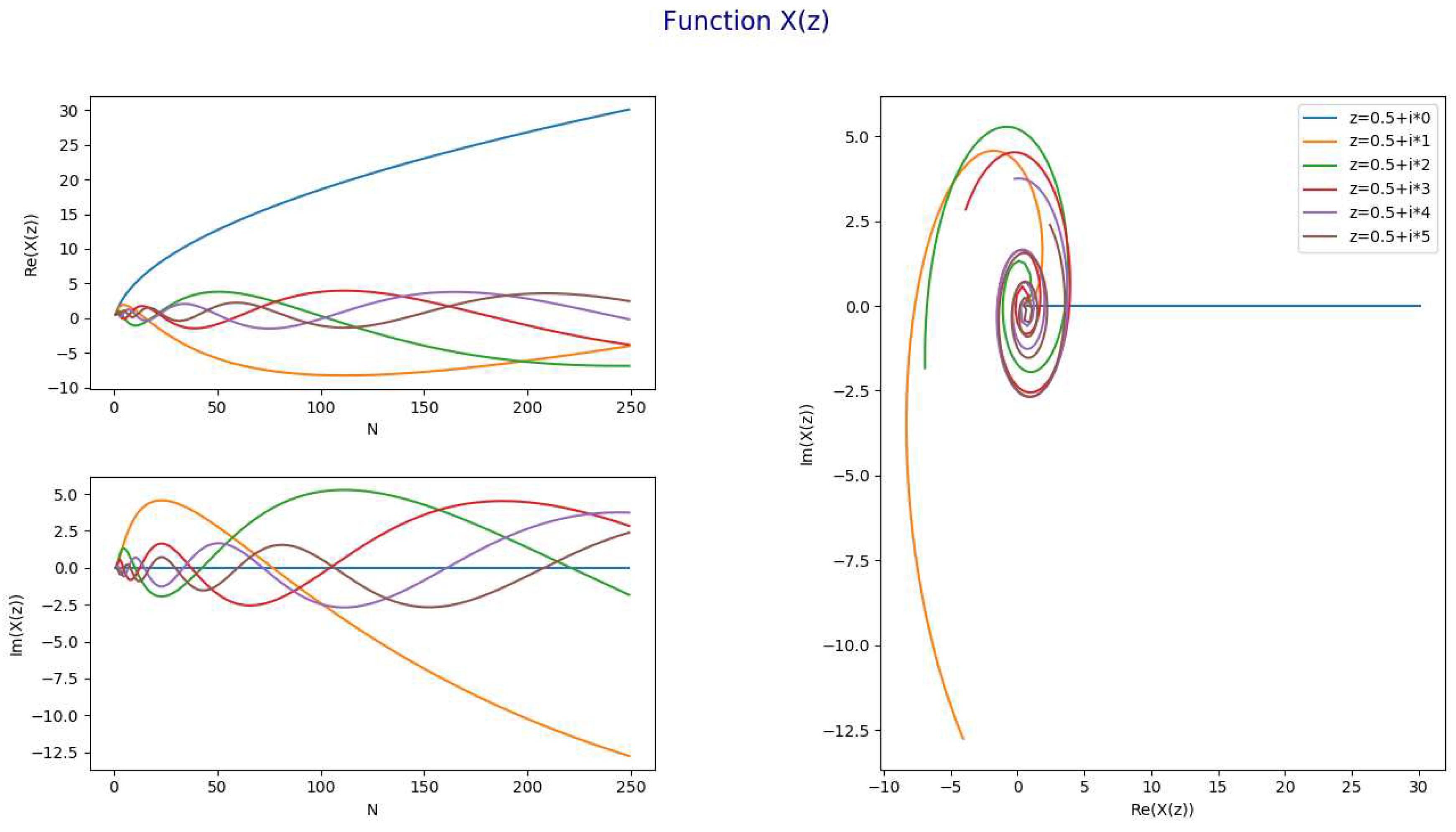
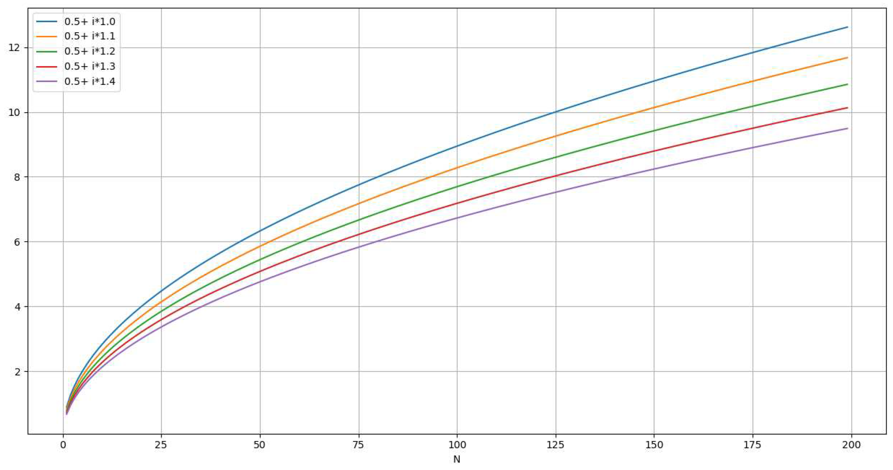
Representation of the function X ( z , n )
The following chart represents X ( z , n ) for a = 1 / 2 and b 1,6   and n = 250 .
Figure 7. X ( z , n )
Preprints 93993 g007
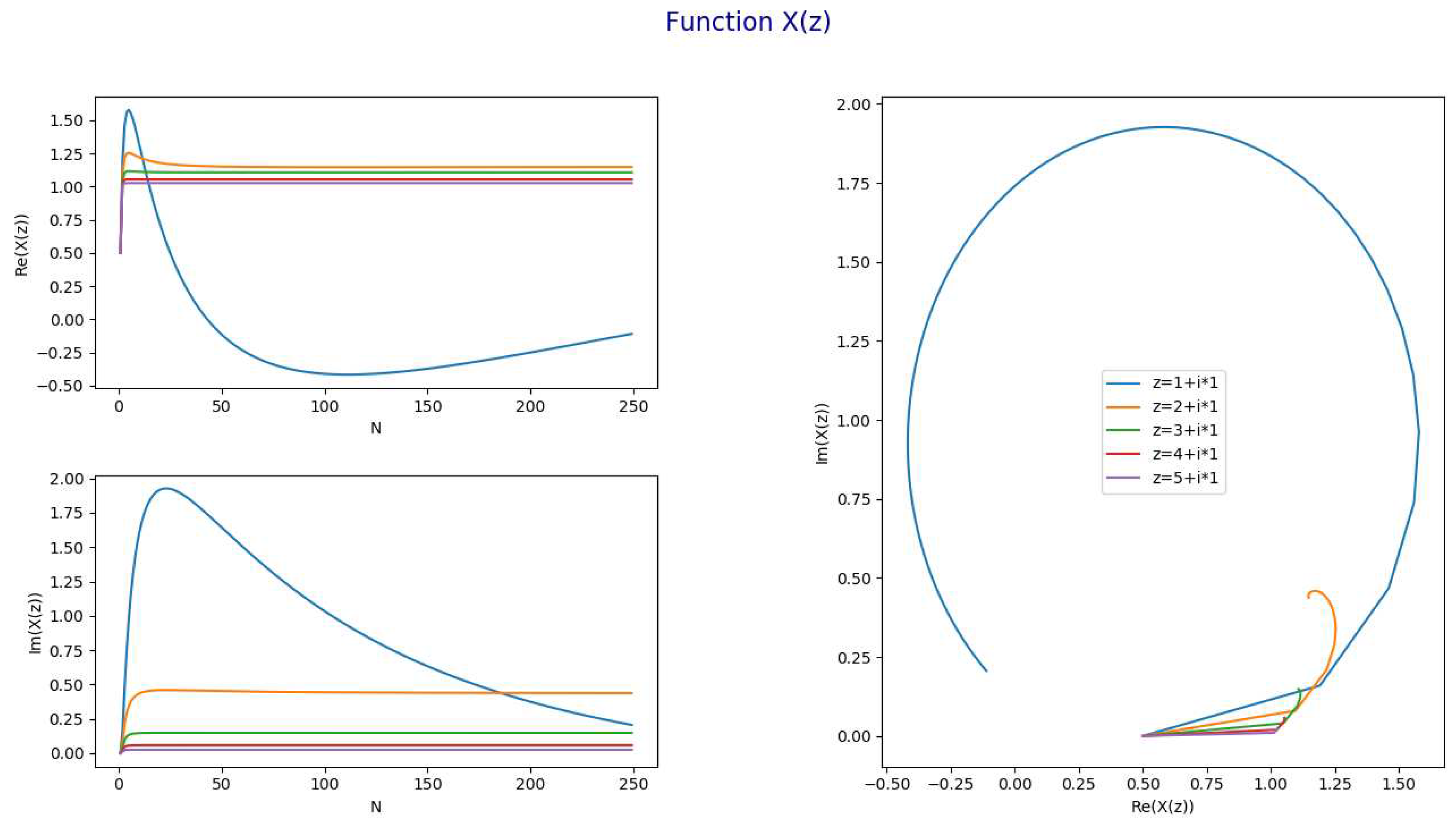
  • The following chart represents X ( z , n ) for a [ 1,6 ]   and b = 1 and n = 250 .
Figure 8. X ( z , n )
Preprints 93993 g008
6.
Representation of the function Y ( z , n )
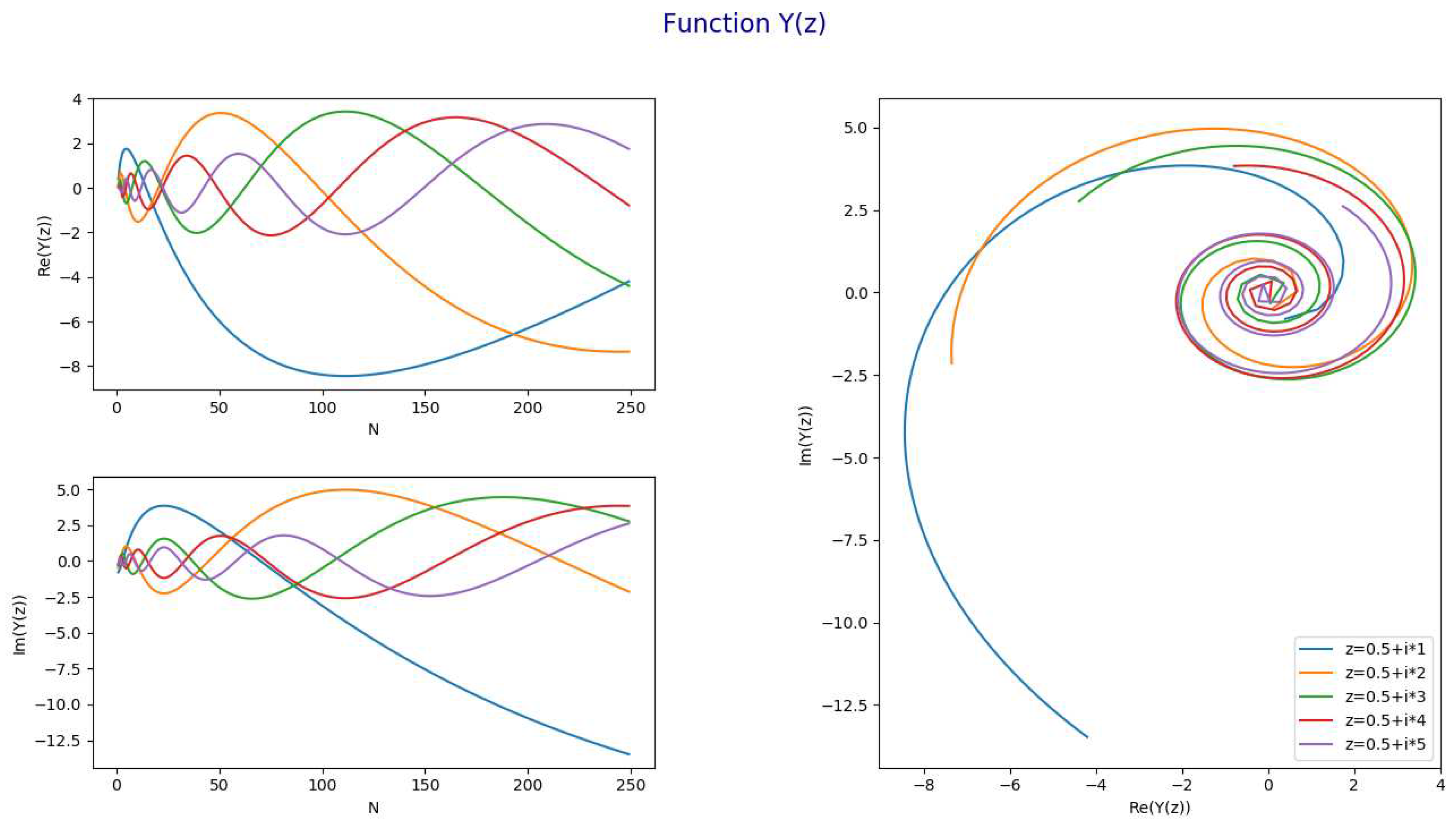
The following chart represents Y ( z , n ) for a = 1 / 2 and b 1,6 and n = 250
Figure 9. Y ( z , n )
Preprints 93993 g009
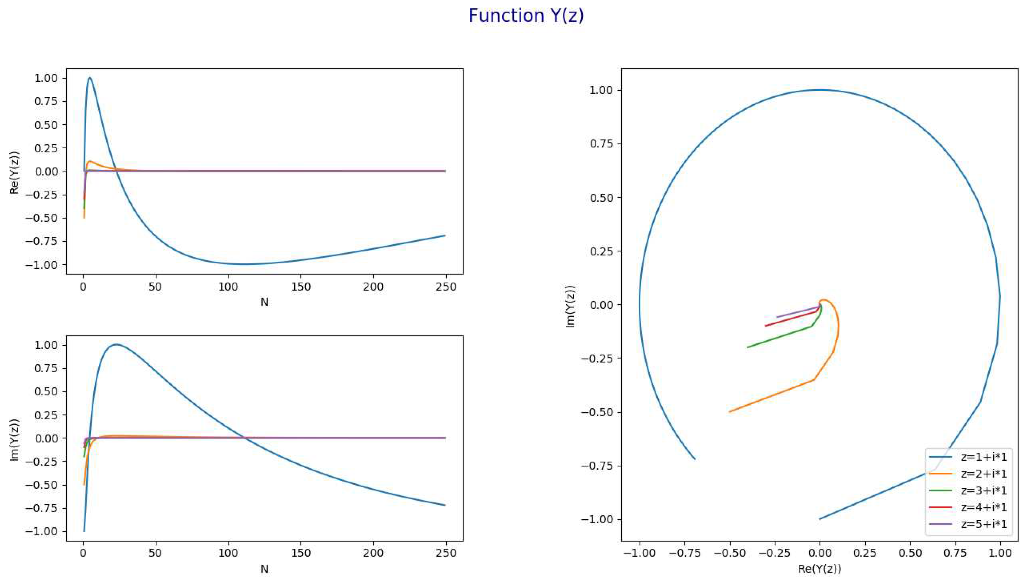
  • The following chart represents Y ( z , n )   for a [ 1,6 ] and b = 1 and n = 250
Figure 10. Y ( z , n )
Preprints 93993 g010
7.
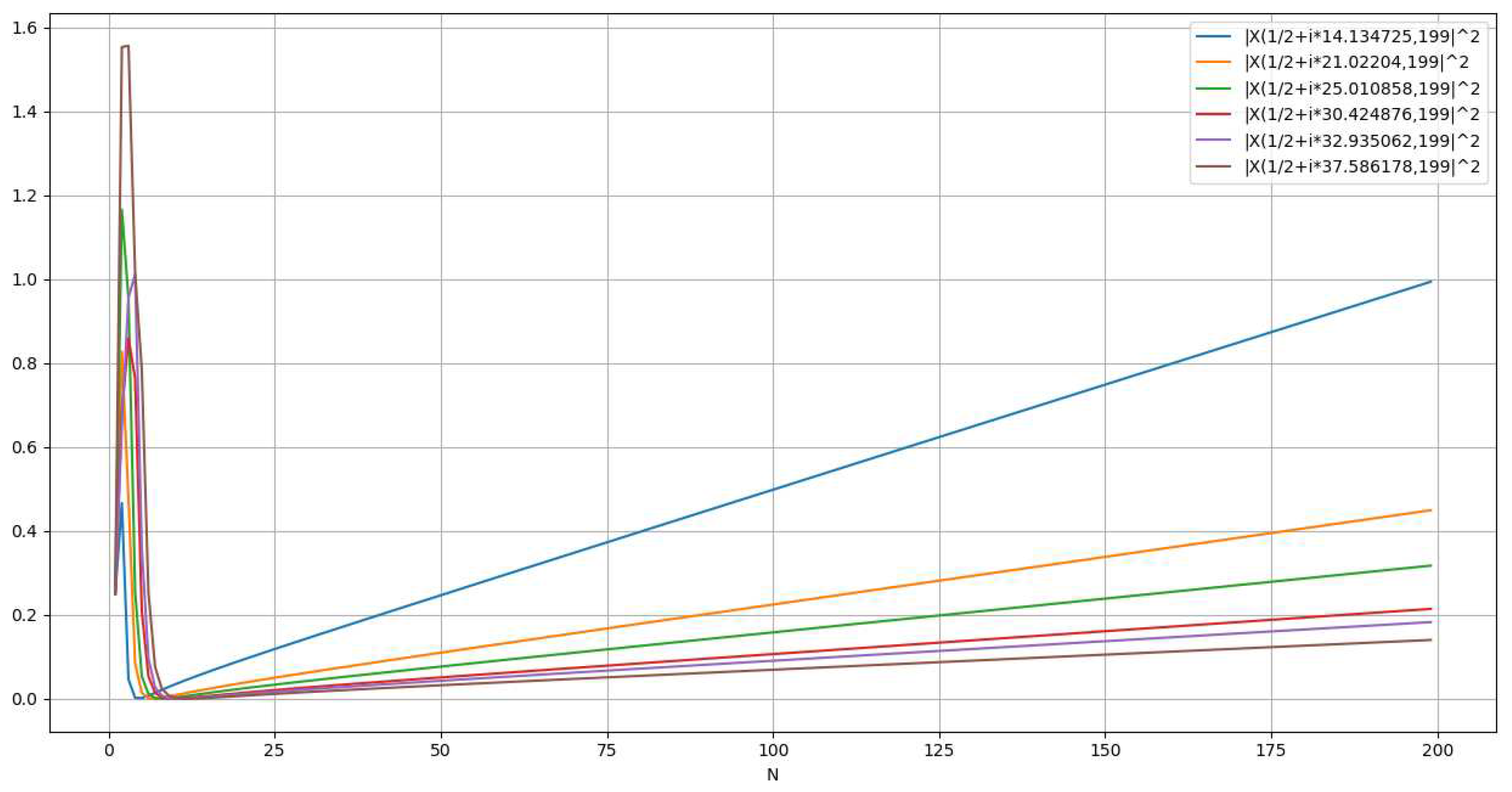
Representation of | X ( z , n ) |
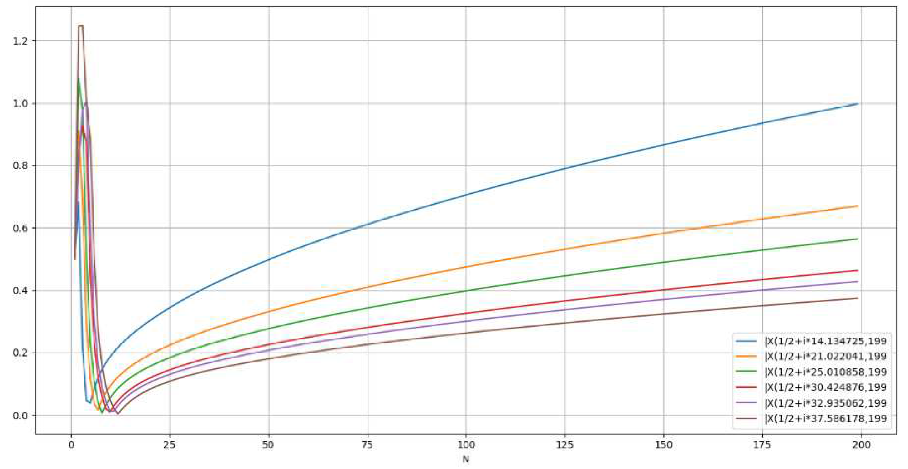
Wave representation for | X ( z , n ) | f o r R e ( z ) = 1 / 2   a n d   I m ( z )   v a r i a b l e . [Figure. 11]
Preprints 93993 i011
  • Parabolic representation for | X ( z , n ) |   f o r   ( z )   a   n o n t r i v i a l   z e r o   o f   R i e m a n n   Z e t a . [Figure. 12]
Preprints 93993 i012
  • Linear representation for | X z , n 2   f o r   ( z )   a   n o n t r i v i a l   z e r o   o f   R i e m a n n   Z e t a . [Figure. 13]
Preprints 93993 i013
8.
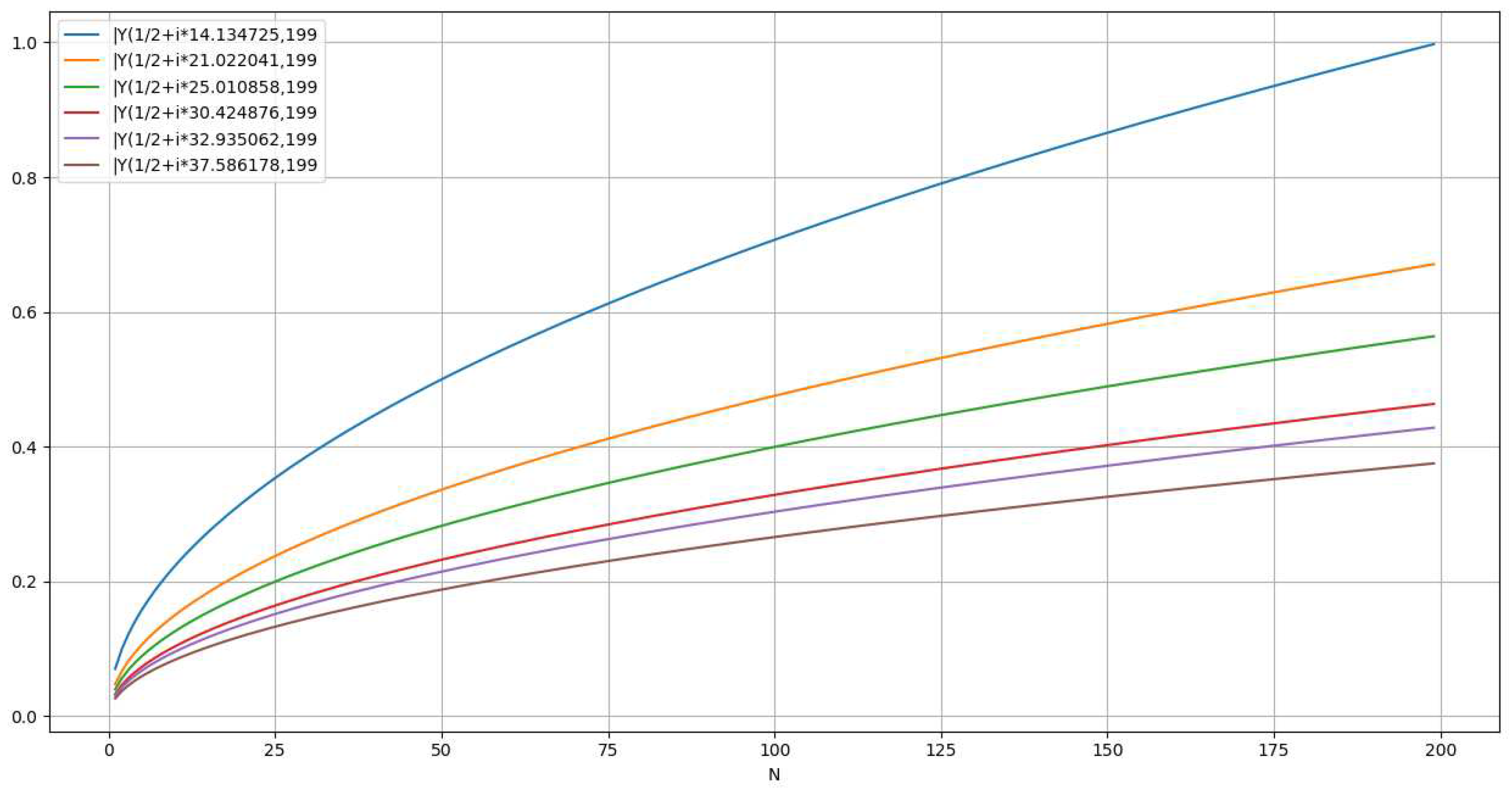
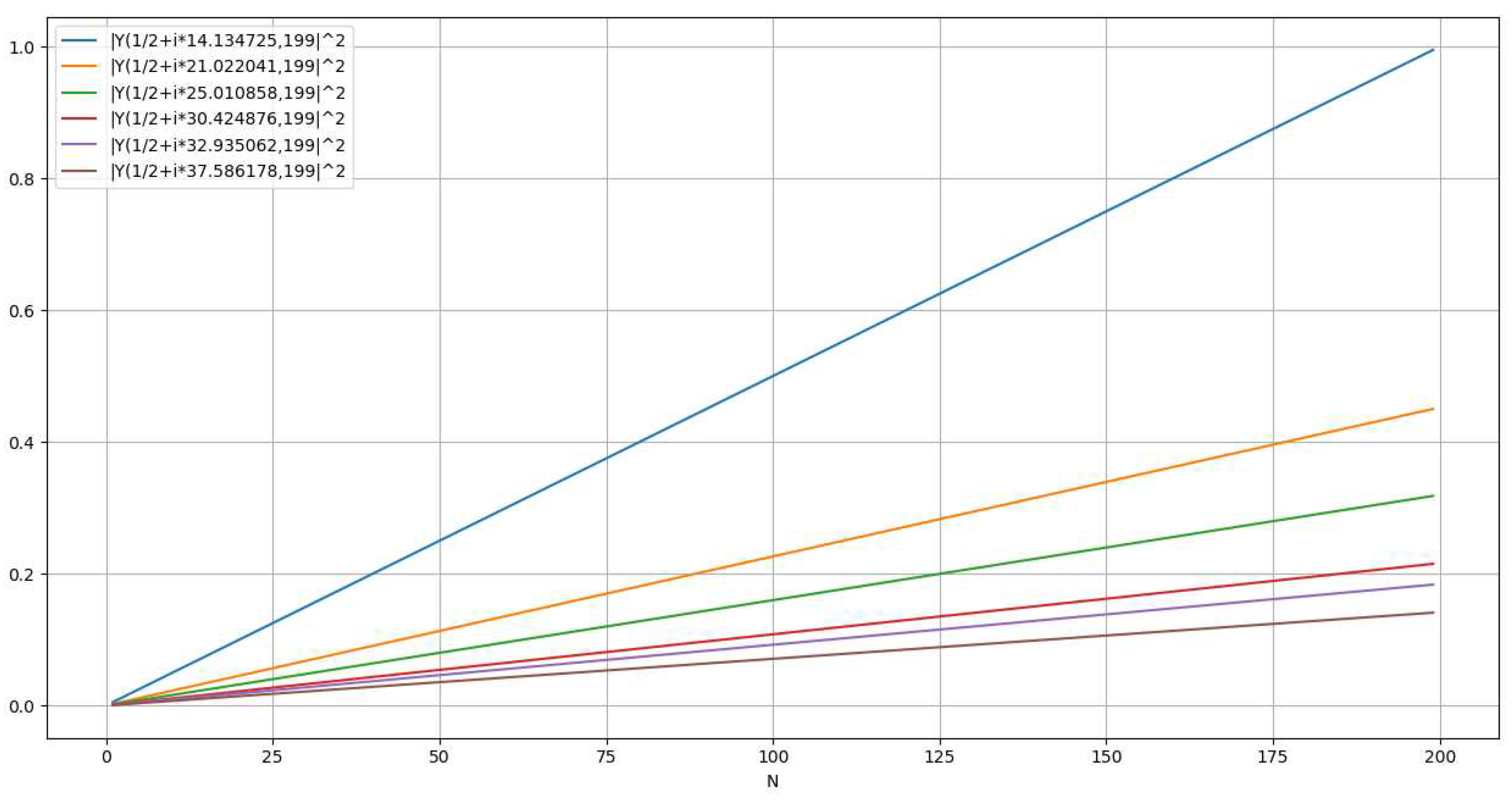
Representation of | Y ( z , n ) |
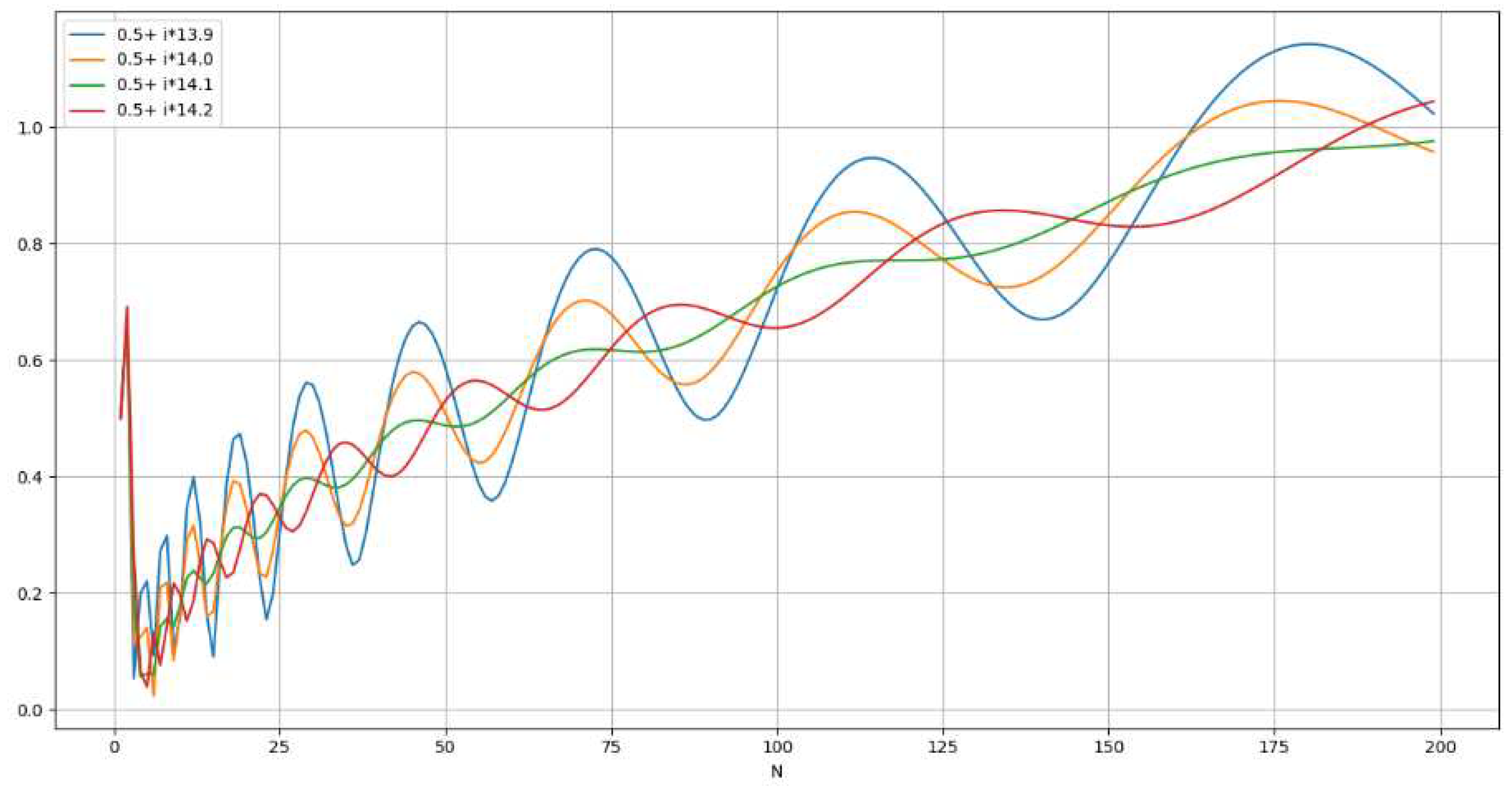
Polynomial representation for | Y ( z , n ) | f o r R e ( z ) = 1 / 2   a n d   I m ( z )   v a r i a b l e . [Figure. 14]
Preprints 93993 i014
  • Parabolic representation for | Y ( z , n ) |   f o r   z a   n o n t r i v i a l   z e r o   o f   R i e m a n n   Z e t a . [Figure. 15]
Preprints 93993 i015
  • Linear representation for Y z , n 2   f o r   z a   n o n t r i v i a l   z e r o   o f   R i e m a n n   Z e t a . [Figure. 16]
Preprints 93993 i016
9.
Conclusion PART 3
Using the defined C-transformation, one can write the Riemann Zeta function as the difference of two functions X(z) and Y(z) for R e z 0 , z 1 . This will provide a new way of analyzing the zeros of the Zeta function, and a new approach to the Riemann Hypothesis.
The decomposition is as follows:
ζ ( z )   =   X ( z )     Y ( z ) , where:
X ( z ,   n )   = k = 1 n k α c o s ( ß ln k ) + 1 2   n α c o s ( ß ln n ) + +   i ( k = 1 n k α s i n ( ß ln k ) + 1 2   n α sin ß ln n
  and:   X ( z ) = lim n X z , n
Y ( z ,   n ) = n 1 α 1 [ 1 α 2 + ß 2 ] [ 1 α cos ß ln n + ß sin ß ln n + + i ( ß cos ß ln n 1 α sin ß ln n ) ]
  and:   Y ( z )   =   lim n Y z , n
Observations:
  • | X ( z , n ) | has a wave representation
  • | X ( z , n ) | becomes a parable when z is a nontrivial zero of Riemann Zeta
  • X z , n 2 becomes a line when z is a nontrivial zero of RZF with slope equal 1 ß 2 + ¼
  • | Y ( z , n ) | has a polynomial representation
  • | Y ( z , n ) | becomes a parable when z is a nontrivial zero of Riemann Zeta
  • Y z , n 2 becomes a line when Re(z)=1/2 with slope equal 1 / ( ß 2 + ¼ )
So, the only common representation for |X(z)| and |Y(z)| occurs when Re(z)=1/2, so
X ( z )     Y ( z ) = 0 if and only if Re(z)=1/2

PART 4: Proof of the Riemann Hypothesis using the decomposition. ζ ( z ) = X ( z ) Y ( z )

1.
Analysis of Absolute Square Y z , n 2
Y z , n 2 = [ (   n 1 α 1 [ 1 α 2 + ß 2 ]   1 α c o s ß l n n + ß s i n ß l n n ) 2   +   n 1 α 1 [ 1 α 2 + ß 2 ]   ß c o s ß l n n 1 α s i n ß l n n 2 ]
Y z , n 2 = n 2 1 α   1 ß 2 + 1 α 2 Polynomial   representation
This could be observed in Figure. 14, 15, 16.
1.1. Y z , n 2 is a straight line if and only if α = 1 2
The slope of Y z , n 2 with respect to n is given by:
s l o p e ( Y z , n 2 )   = d ( Y z , n 2 ) / d n
Which equals to:
d ( Y z , n 2 ) / d n =   2 1 α   n 1 2 α     1 [ ß 2 + 1 α 2 ]  
Y z , n 2 can only be a line when the slope is constant, which can only happen if and only if:
( 1 2 α ) = 0
therefore:
Y z , n 2   is   a   straight   line   if   and   only   if   α = 1 2
1.2. Summary for Y z , n 2 for α = 1 2 :
 ⇨
the slope Y z , n 2 is constant if and only if α = 1 2
 ⇨
When α=1/2, Y z , n 2 = n [ ß 2 + 1 4 ]
 ⇨
The slope for Y z , n 2 is 1 [ ß 2 + 1 4 ] for α = 1 2
2.
Analysis of Absolute Square
X z , n 2
X z , n 2 = ( 1 2 n a cos ß ln n + k α cos ß ln k ) 2 + ( 1 2 n a s i n ( ß ln n ) + k α sin ß ln k ) 2
Applying properties of infinite series (Kopp):
X z , n 2   = 1 4 n 2 a ( cos 2 ß ln n + sin 2 ( ß ln n ) ) + ( k α cos ß ln k ) 2 + ( k α sin ß ln k ) 2 + +   n a [ c o s ( ß ln n ) k α cos ß ln k ] + + n a [ s i n ( ß ln n ) k α sin ß ln k ]
X z ,   n 2 = k = 1 n j = 1 n k α j α cos ß ( ln k j + k = 1 n k 2 α + + 1 4 n 2 a + n a [ c o s ( ß ln n ) k α cos ß ln k ] + + n a [ s i n ( ß ln n ) k α sin ß ln k ]
One can express the previous expression replacing:
R n = 1 4 n 2 a +   n a   [ c o s ( ß ln n ) k α cos ß ln k + s i n ( ß ln n ) k α sin ß ln k ]
With:
lim n R n = 0 if   α > 0 therefore ,
X z , n 2 = k = 1 n j = 1 n k α j α cos ß *ln k j + k = 1 n k 2 α + R n  
When X z , n 2 is represented graphically, one can observe that:
-
X z , n 2 is a wave that converges when n and α>1 (Figure 17)
-
X z , n 2 is a wave that does not converge when n and α<1 (Figure 18)
-
X z , n 2 is a wave that collapses to a line when n and α=1/2 and ß=Im( ζ ( z ) ) (Figure 19) where z* is a nontrivial zero of RZF.
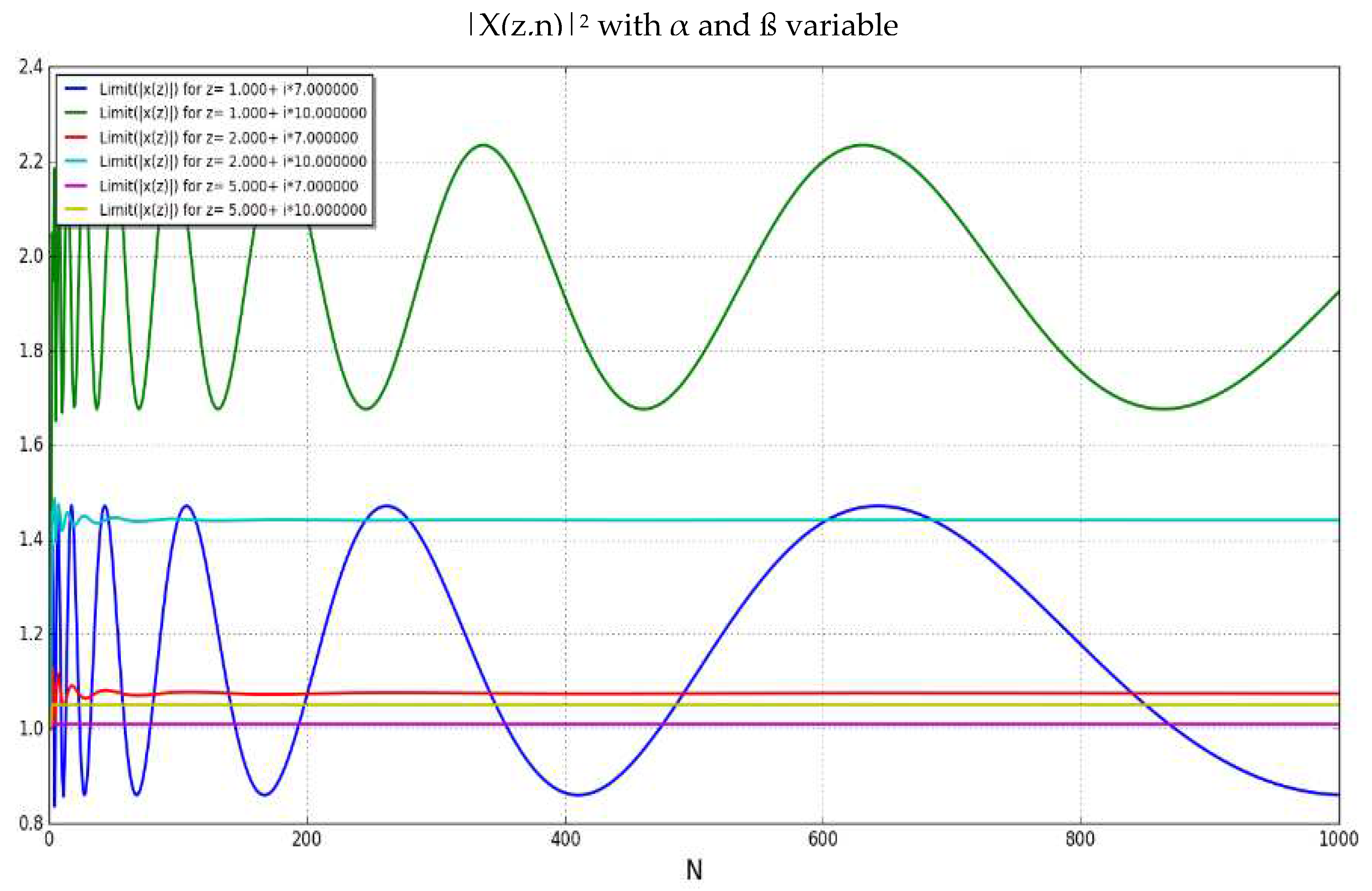
2.1. X z , n 2 converges when n  and α>1 to ζ α , ß 2
The limit of X z , n 2 outside the critical strip [0,1] can be calculated using [16]:
lim n X z , n 2     = lim n k = 1 n j = 1 n k α j α cos ß ( ln k j
As one can see in some examples in the following table where z=α+iß:
Table 7.  
Table 7.  
α ß lim n X z , n 2 ζ α , ß 2
1.0 7 1.074711506185445 1.074756
1.0 10 1.4413521753699579 1.441430
2.5 7 1.0093487944300192 1.009349
2.5 10 1.0507402208589398 1.050740
lim n X z , n 2 = ζ z 2 = ζ α + ß i ζ α ß i       f o r   α > 1
And also, in the following Figure 20:
One can observe that the graphs for α=1 do not converge while graphs for α>1 they all converge.
This observation can be used to prove that there are no zero values of ζ(z) for z with Re(z)>1.
2.2. X z , n 2 diverges when n  for α 1
X z , n 2 diverges when n for α<1 because of [16] and [17]:
| cos ß ( ln k j | < 1
And:
k = 1 n j = 1 n k α j α   d i v e r g e s   f o r   α < 1
Therefore:
lim n X z , n 2     = k = 1 n j = 1 n k α j α cos ß ( ln k j   d i v e r g e s   f o r   α < 1
2.3. X z , n 2 does not collapse to any polynomial function X z , n 2 = C n t   f o r   t > 1 ,   a n d   C   c o n s t a n t
One can prove it with a reduction to absurd.
Let’s assume that X z , n 2 = C n t   f o r   t > 1 where C and t integers C>0 and t>0
If   X z , n 2 = C n t   then :
lim n X z , n 2 / n t   =   C
But:
lim n X z , n 2 / n t     = 1 n t lim n k = 1 n k 2 α + 1 n t k = 1 n j k n k α j α cos ß ( ln k j
And:
1 n t lim n k = 1 n k 2 α = 0       f o r   t > 1
1 n t k = 1 n j k n k α j α cos ß ( ln k j = 0   f o r   t > 1
So, C must be 0 which is an absurd.
2.4. X z , n 2 collapses to a straight-line X z , n 2 = C n       i f   R e ( z ) = 1 / 2
The proposition says that the following limit exists only for Re(z) = 1/2;
lim n ( X z , n 2 /   n )   =   S
Using the expression:
lim n ( X z , n 2 /   n ) = lim n 1 n ( k = 1 n k 2 α + k = 1 n j k n k α j α cos ß ( ln k j )
2.4.1. For α>1/2, one can see that  lim n ( | x ( z ,   n ) | 2 / n ) = 0:
    lim n 1 n ( k = 1 n k 2 α ) = 0 because 2α>1 and the series is convergent
lim n 1 n k = 1 n j k n k α j α cos ß ( ln k j ) < lim n 1 n k = 1 n j k n ( k α j α ) < lim n 1 n ( k = 1 n k 2 α )
So:
lim n 1 n k = 1 n j k n k α j α cos ß ( ln k j = 0
2.4.2. For α<1/2, one can see that lim n ( X z , n 2 / n ) =   as:
lim n 1 n ( k = 1 n k 2 α ) < lim n 1 n n 1 n = lim n 1 n =   0
And:
lim n 1 n k = 1 n j k n k α j α cos ß ( ln k j ) > lim n ( 1 n   n 2 1 n 2 α ) =
Where the summations are replaced by the number of elements in the matrix (n x n) times the smallest value in each row (1/n) then 1>(2-1-2α)>0 when α<1/2
2.4.3. Limit for α=1/2.
When α=1/2, one can express ( X z , n 2 /n) as:
lim n ( X z , n 2 / n )   = = lim n 1 n ( k = 1 n k 1 + k = 1 n j k n k 1 / 2 j 1 / 2 cos ß ( ln k j ) =   lim n 1 n k = 1 n k 1 +   lim n 1 n ( k = 1 n j k n k 1 / 2 j 1 / 2 cos ß ( ln k j )   = =   0   +   lim n 1 n ( k = 1 n j k n k 1 / 2 j 1 / 2 cos ß ( ln k j ) =   =   lim n 2 n n ( j = 1 n 1 n 1 / 2 j 1 / 2 cos ß ( ln n j ) = =   lim n 2 (   n 1 2   j = 1 n 1 j 1 2 cos ß ( ln n j ) =
Using the integral approximation of the infinite series
= 2 l i m n 2 n cos ß ln n n 2 ß s i n ( ß l n ( n n ) 4 ß 2 + 1   n 1 2 = 2   2 n 4 ß 2 + 1 n 1 2 = 2   2 4 ß 2 + 1 =   1 ß 2 + 1 / 4
So, if lim n ( X z , n 2 / n )   exists will be equal to:
lim n ( X z , n 2 / n ) =   1 ß 2 + 1 / 4
            if z=1/2+iß
And this limit can only exist when X z , n 2 is monotonous which means that the curve will cross the x-axis only once.
X z , n 2 = k = 1 n j = k n k 1 2 j 1 2 cos ß ( ln k j = 2 n a j = 1 n 1   j a cos ß ( ln x j )
3.
Calculating the zeros of X z , n 2
Let’s define the function C 2 n , a , b =     X z , n 2   in R (where z=a+bi) such that:
C 2 n , a , b = 2 n a j = 1 n 1   j a cos b ( ln n j )
With the following wave representation for C 2 n , a , b :
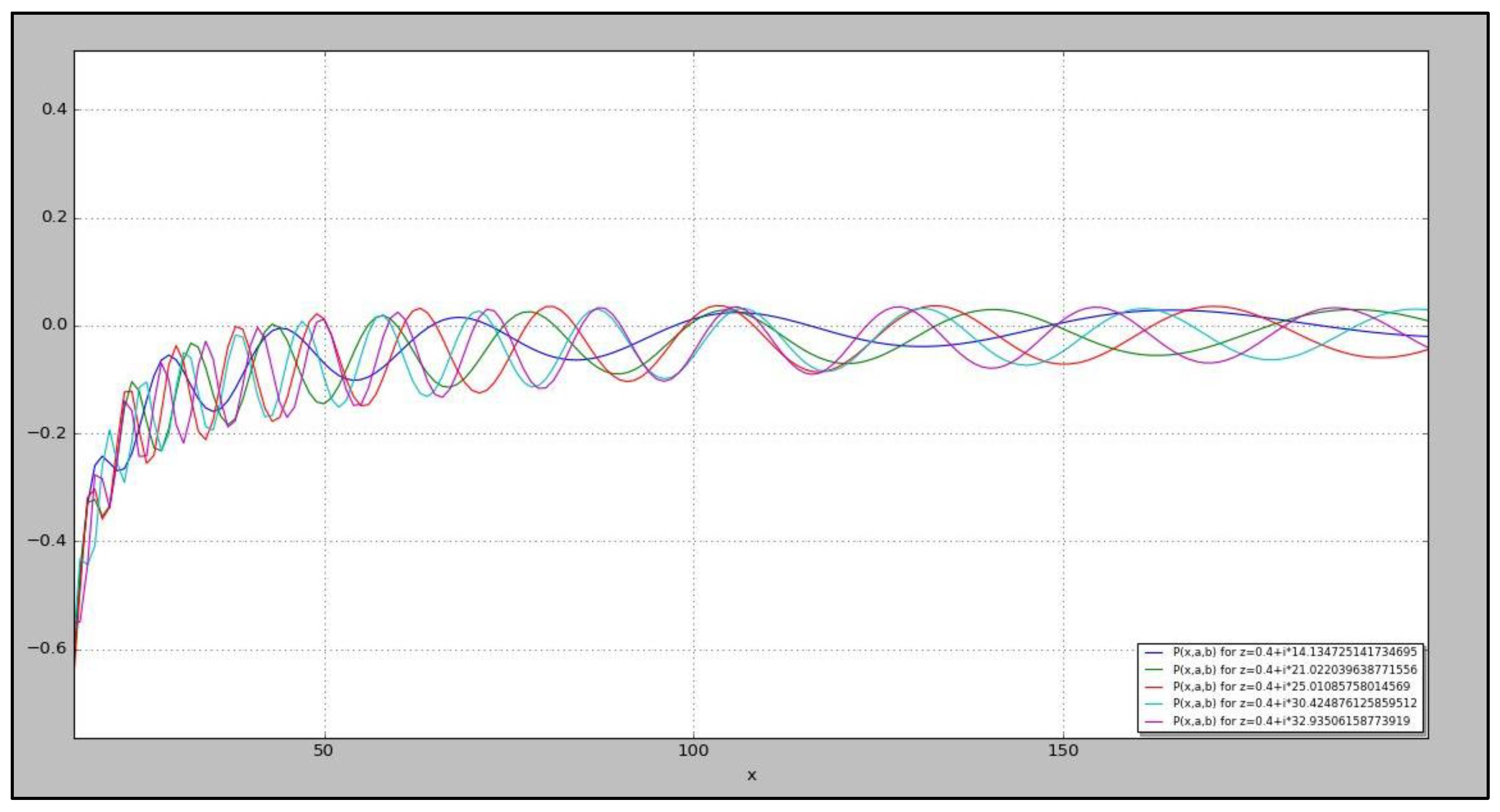
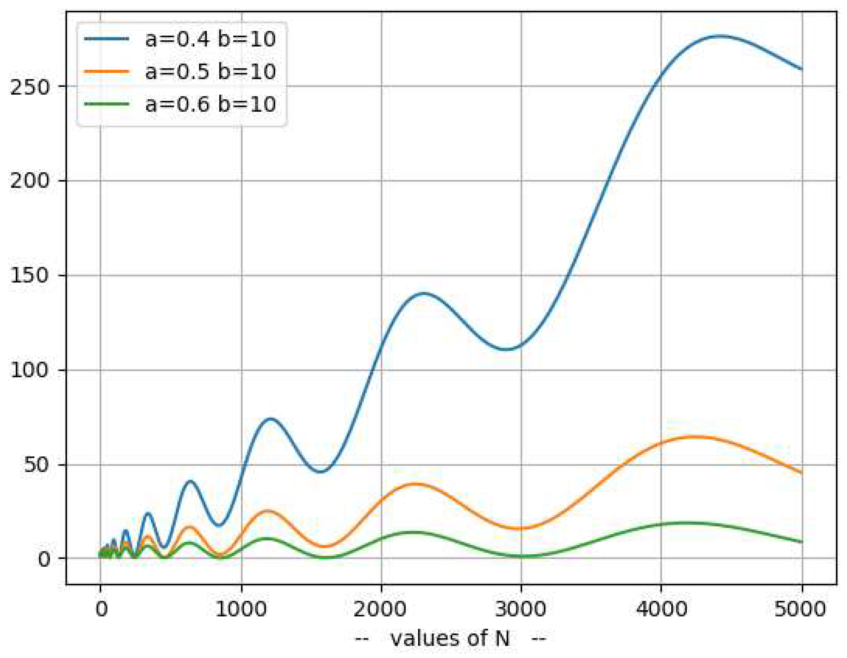
Figure 21. C 2 x , a , b for a=0.4 and variable b.
Preprints 93993 g021
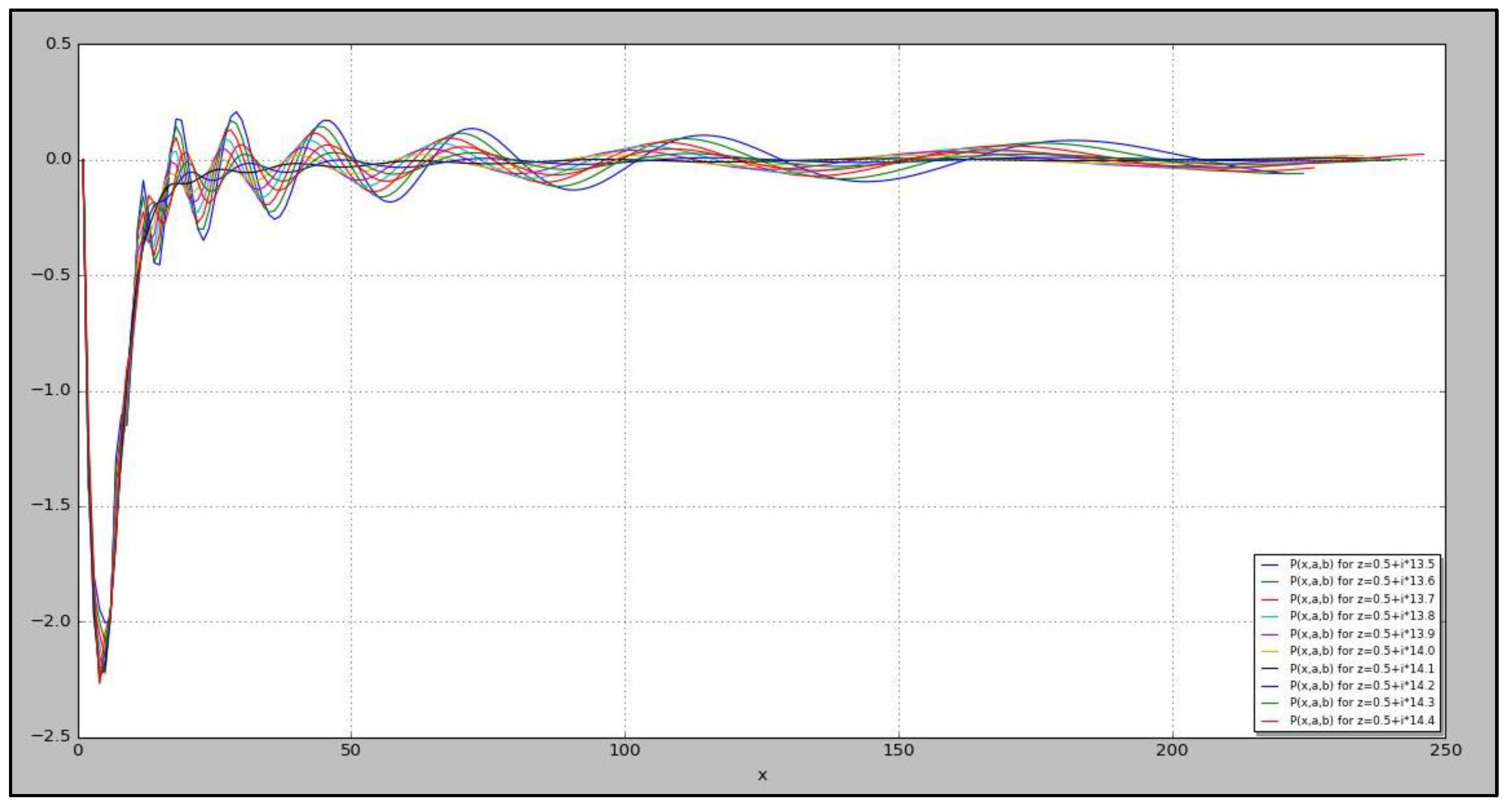
Figure 22. C 2 n , a , b for a=0.5 and variable b.
Preprints 93993 g022
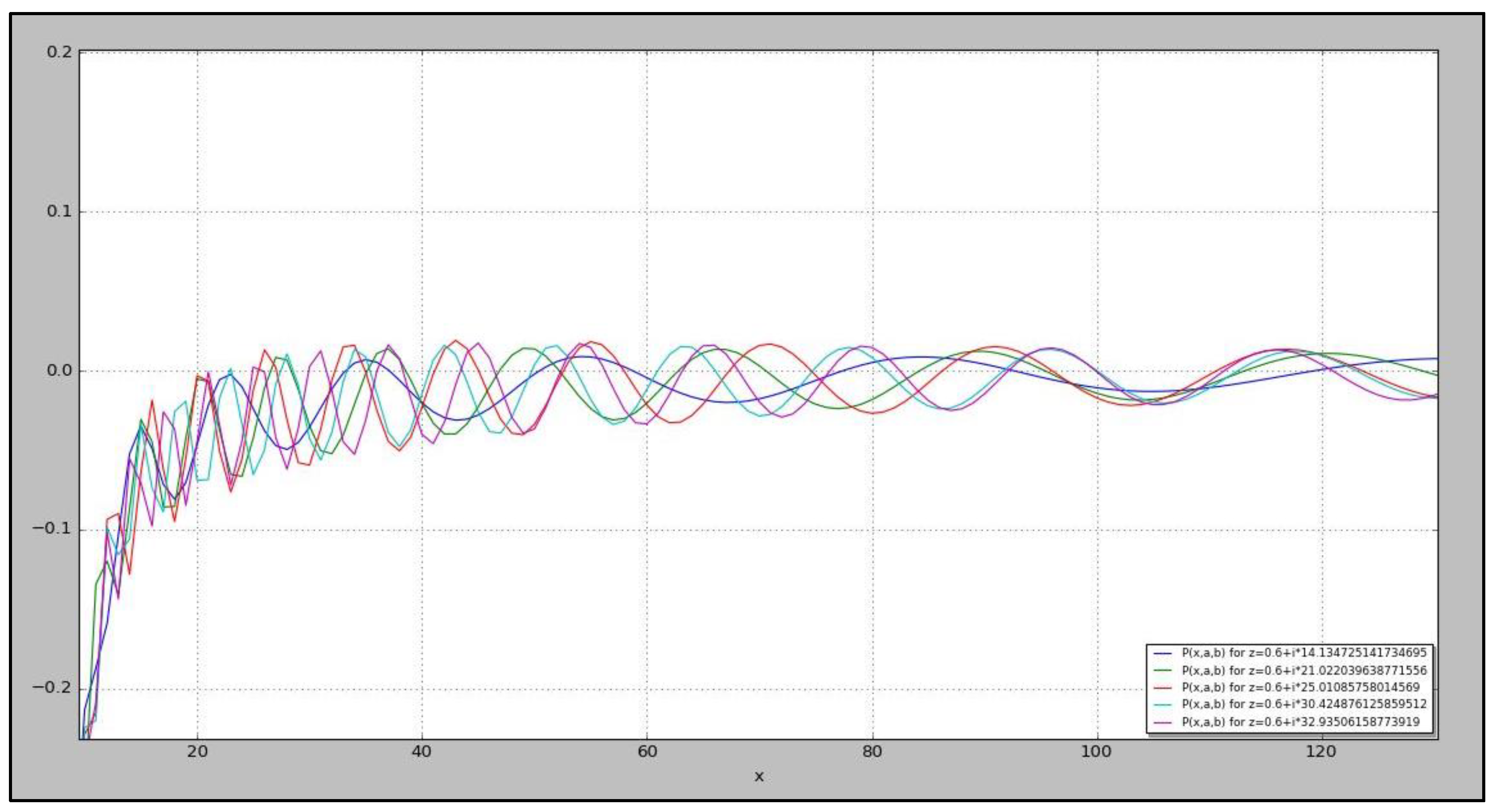
Figure 23. C 2 n , a , b for a=0.6 and variable b.
Preprints 93993 g023
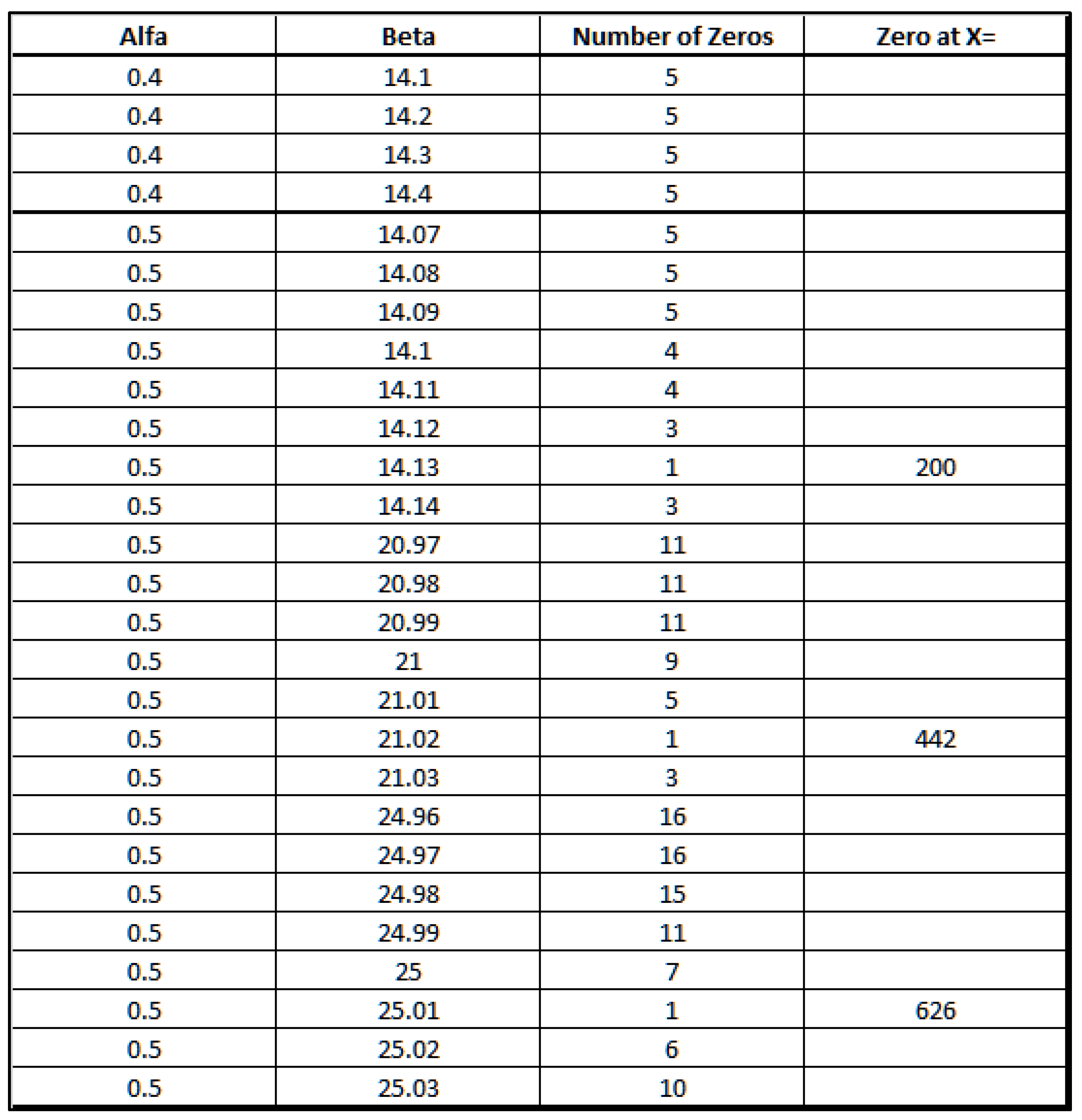
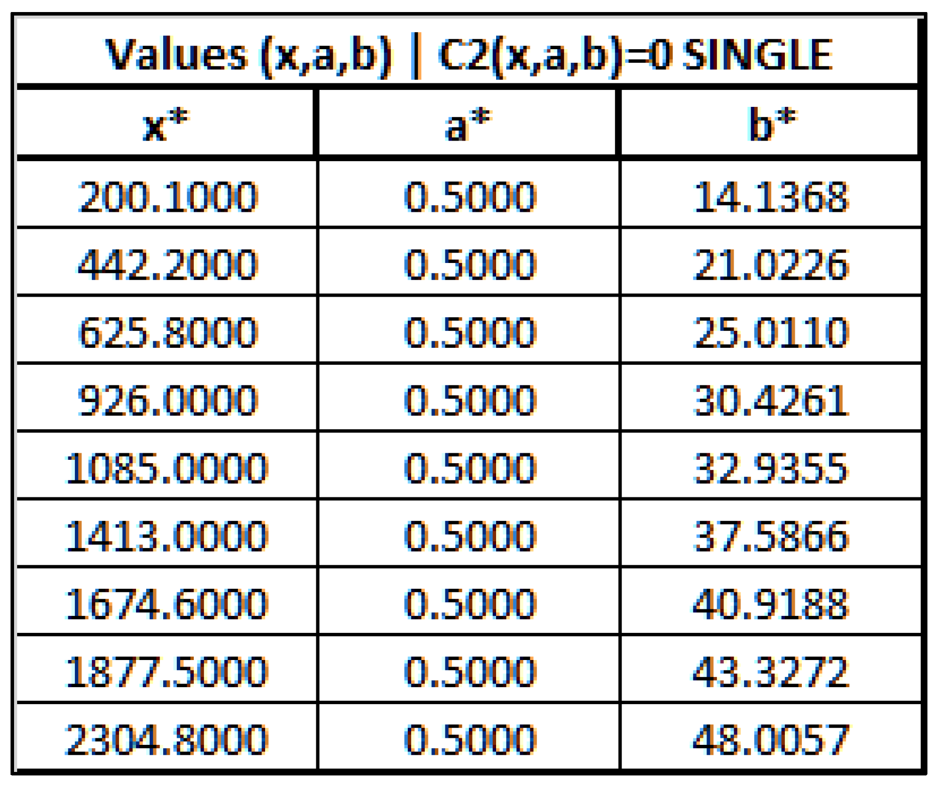
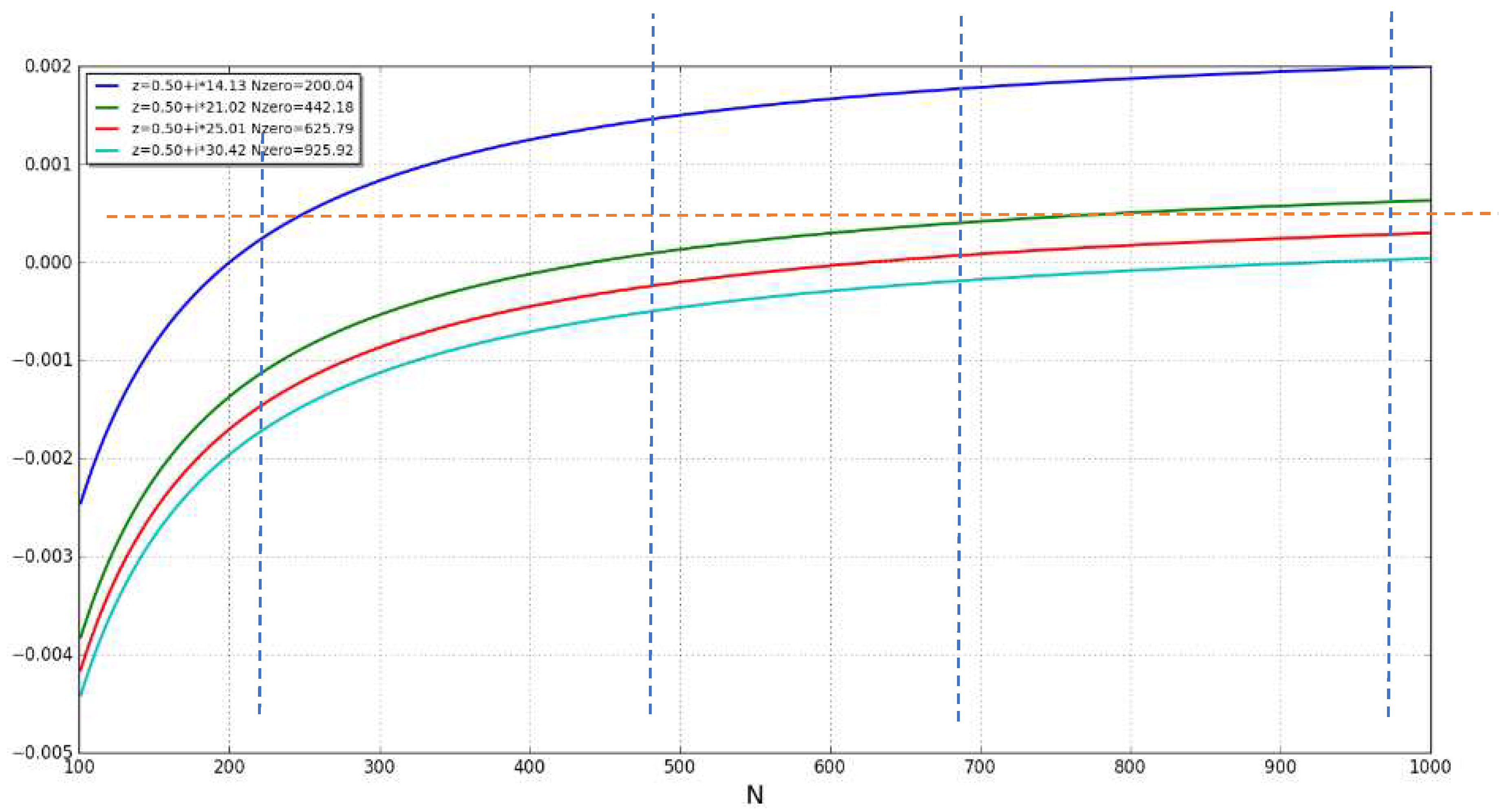
As a wave, C 2 n , a , b can have one or more zeros. For C 2 n , a , b to have only one zero, it must cross the axis y=0 only once, which means that the wave collapses to a polynomial line. A numeric method has been created and coded (Python) to find the values of n , a , b such that C 2 n , a , b =0. The following table shows an example of those calculated values, where x=n, a=Alfa, and b=Beta:
Table 8. Number of Zeros of C 2 x , a , b for different values of a=Alfa, and b=Beta.
Preprints 93993 i002
The calculations for a 0,1 and b [ 1 ,   100 ] only found single zeros for C 2 x , a , b for values of a = 0.5 as shown in the following table that summarizes the single zeros found in those intervals:
Table 9. List of first Zeros of C 2 x , a , b .
Preprints 93993 i003
One can observe that:
i f C 2 x , a , b = 0 a = 1 / 2 b =   I m ( z )                 w i t h   ζ ( z ) = 0 ( a , b ) a r e   t h e   N o n t r i v i a l   Z e r o s   o f   ζ ( z )   i n   t h e   c r i t i c a l   l i n e . x = b 2 + 1 4
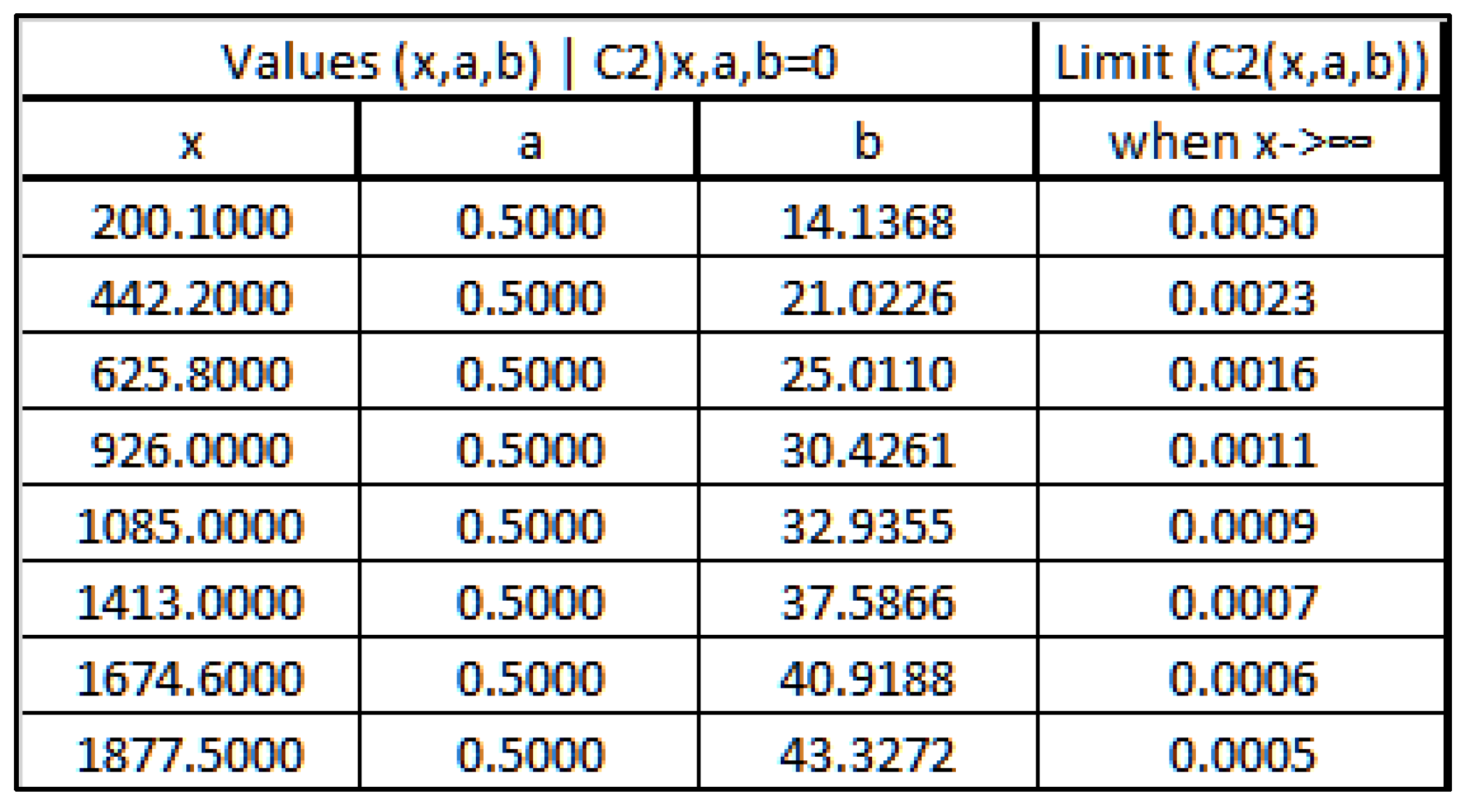
And the calculated values of lim x C 2 x , a , b for the values of (a,b) from Table 9 are:
Table 10. Limit of C 2 x , a , b for b in Table 10 and x->∞.
Preprints 93993 i004
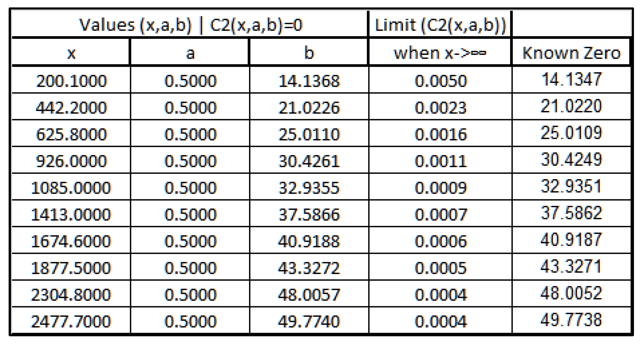
Table 11. Comparing “b” calculated with known zeros of ζ(z).
Preprints 93993 i005
Therefore, X z , n 2 = C n , a , b has the following special properties for all (a,b) such that ζ(a+bi)=0.
if S=   1 b 2 + 1 / 4
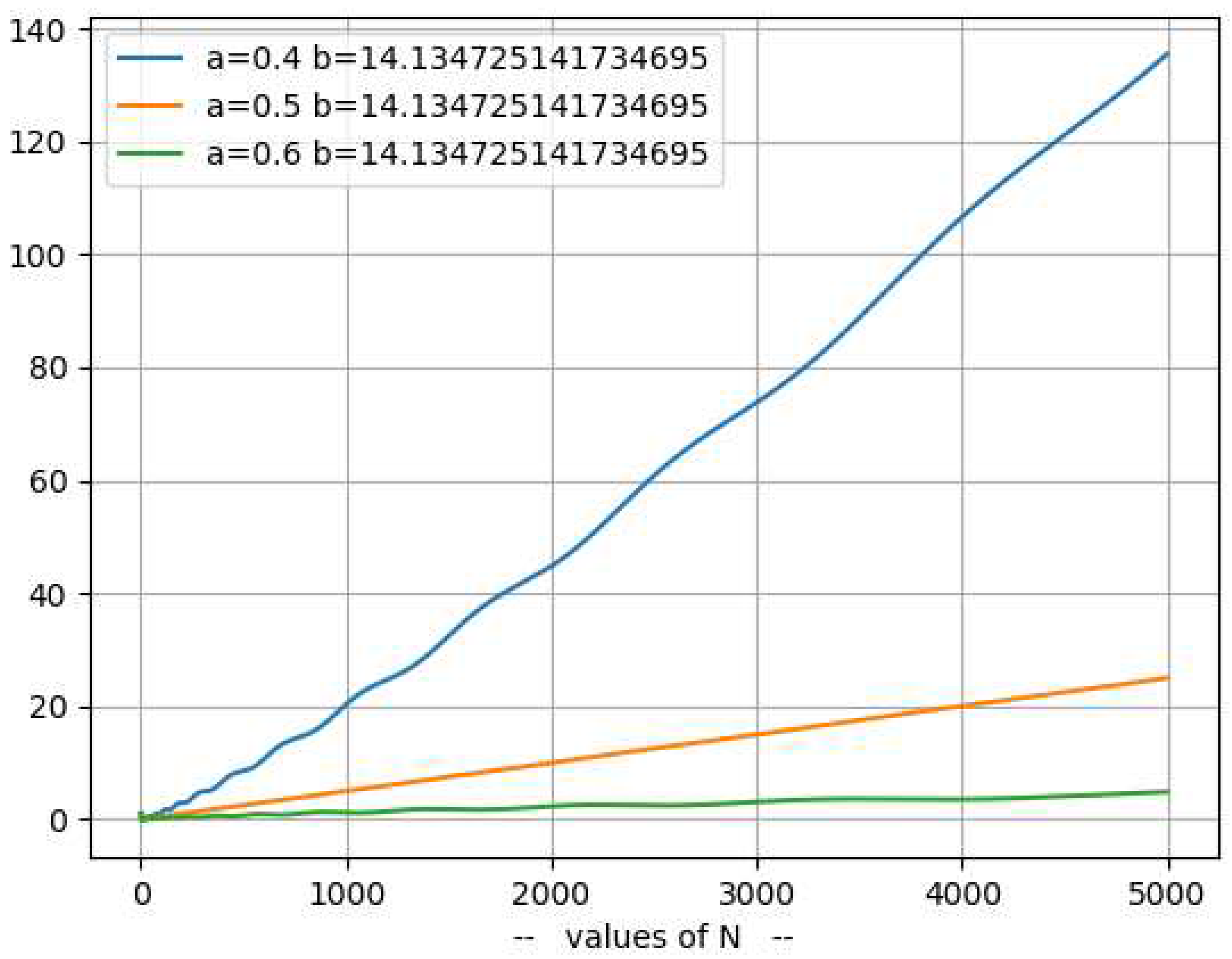
C 2 n , a ,   b =   0   w h e n   x = 1 S ,     a = 1 2 ,       b = I m z   w i t h z a n o n t r i v i a l z e r o o f ζ ( z )
lim x C 2 n , 1 2 , b = S
Graphically:
Figure 24. C 2 n , 1 / 2 , b such that ζ(1/2+b*i)=0.
Preprints 93993 g024
4.
Theorem: For Re(z)≥0, if z* is a nontrivial zero of ζ(z), then Re(z*)=1/2
Proof:
From [10], [11], [12]: ζ(z) = X(z) − Y(z) for Re(z)>0, z≠1
From [13]: |Y(z, n)|2 is always a polynomial line.
From [14]: |Y(z, n)|2 is only straight line if and only if Re(z)= ½
Y z 2 = lim n Y z , n 2 tends to a straight line with slope 1 [ ß 2 + 1 / 4 ]
From [15]: |X(z, n)|2 is a wave function that has only one polynomial representation in the form of a straight line if and only if Re(z)= ½ [18] and for certain values of Im(z)=ß* calculated using [19]. These values of ß* coincide with the imaginary parts of the nontrivial zeros of Riemann Zeta z*, so:
   X z 2 = lim n X z , n 2 tends to a straight line with slope 1 [ ß 2 + 1 / 4 ]
  when Re(z)=1/2 and ß=NTZ of RZF
Therefore X z 2 = Y z 2 and X z = | Y z | only occur when Re(z*) = ½
As ζ(z)=X(z)-Y(z), therefore all zeros of ζ(z) for z>=0, z≠1 have Re(z)=1/2. [QED]
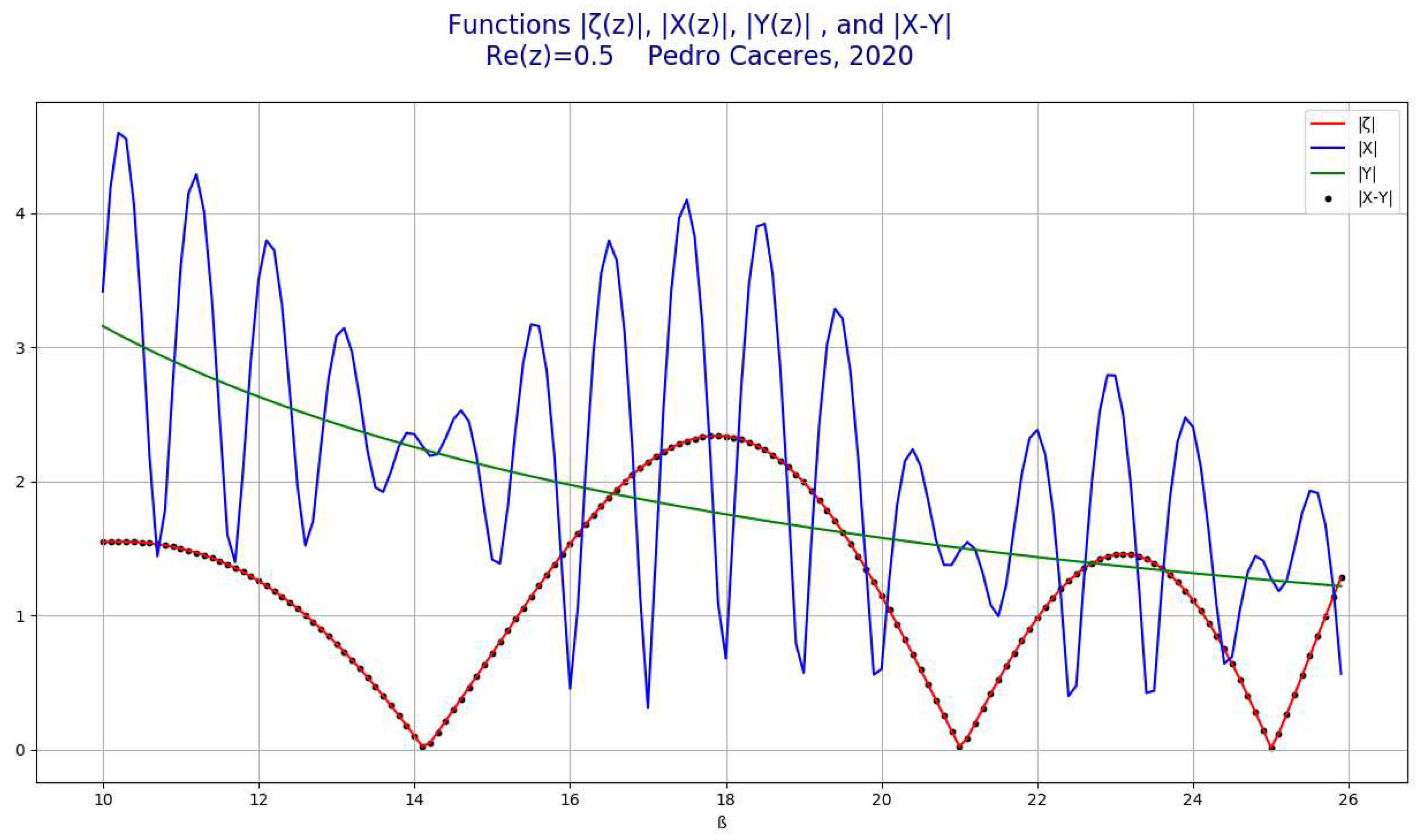
Figure 25. for ζ(z)=X(z)-Y(z)=0 -> |X(z)| = |Y(z)| for Re(z) = 1/2,.
Preprints 93993 g025

PART 5: On the distribution of the zeroes of the RZF in the critical line

1.
From [17] one can write:
X ( z ,   n )   =   ( k = 1 n k 2 α + k = 1 n j k n k α j α cos ß ( ln k j )
therefore, the limit of ( | X ( z , n ) | 2 / n
lim n ( | X ( z , n ) | 2 / n ) = lim n 1 n k = 1 n k 2 α + k = 1 n j k n k α j α cos ß ( ln k j
From [18], if lim n ( | X ( z , n ) | 2 / n )   exists will be equal to:
lim n ( X z , n 2 / n )   =   1 ß 2 + 1 / 4 i f     z = 1 2 + i ß
2.
Calculating the nontrivial zeros of ζ(z) using the Harmonic function
From the previous equations, and for any z = 1 2 + ß i , a nontrivial zero of Zeta in the critical line α=1/2, one can write:
k = 1 n k 1   n ( ß 2 + 1 4 )     k = 1 n j k n k 1 / 2 j 1 / 2 c o s ( ß ( ln k j )   when   n
Where H n =   k = 1 n k 1 is the Harmonic function. One can simplify the expression by creating functions O n   a n d   P ( n ) :
O n =   k = 1 n j k n k 1 / 2 j 1 / 2 c o s ( ß ( ln k j
And
P n = n ( ß 2 + 1 4 )
From the definition of limit, one can write that for any ε arbitrarily small, there exists and N such that for any n>N:
H n O n + P n <   ε
If H n = O n + P n , then [20] can be written as:
H n H n <
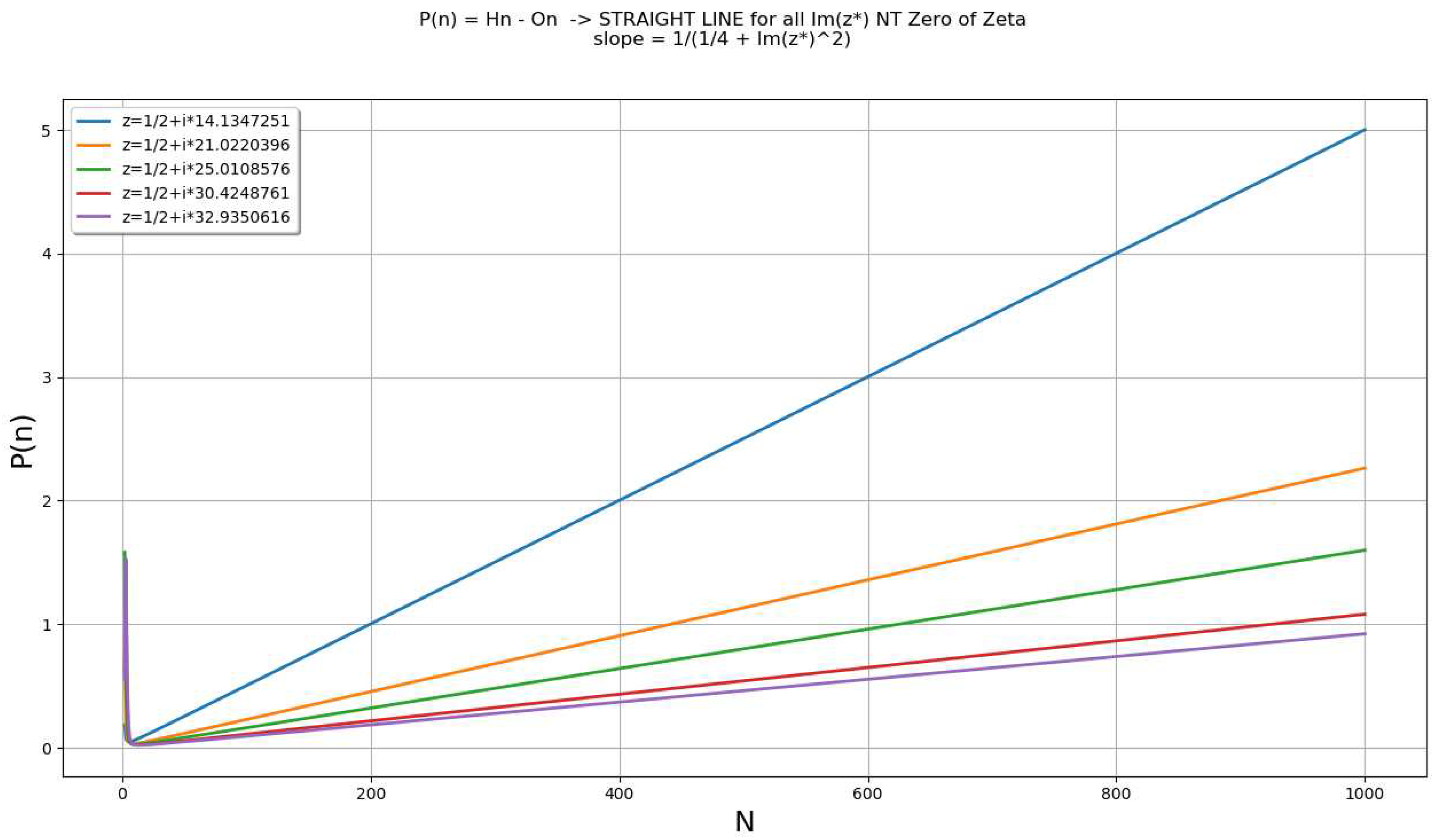
The following chart shows the representation of H(n), O(n), and P(n) [P(n) is a straight line with slope 1 ( ß 2 + 1 / 4 ) ]:
Figure 26. Straight Lines P(n).
Preprints 93993 g026
The equation [20] can be used to create an algorithm to find the nontrivial zeros of zeta in the critical line without knowing any of them based on their connection to the Harmonic function.
An example of a Python code to calculate the zeros of zeta in the critical line with 1 decimal places accuracy based on [20]:
# __Python 3.7
# __Pedro Caceres__ 2020 Feb 17
#Rough code to find zeros of Riemann Zeta using the Harmonic function
harmo   = 0
epsilon = 0.01
nn      = 50
 
for j in range(1,nn):
    harmo += 1 / j
print('Harmonic(',nn,')=', harmo)
 
for b in range (1,500):
    b = b / 10
    a1   = nn/((1-alfa)**2 + b**2)
    b1 = 0
    for k in range(1,nn):
        for j in range(1,nn):
            if j!=k:
                b1 += (k*j)**(-alfa) * m.cos(b * m.log(k/j))
    h1=a1-b1
 
    if abs(h1-harmo) < epsilon:
        print('------> Solution beta=',b, ' ... and->', h1-harmo)
#end_of_code
This code tends the following results:
Harmonic( 50 )= 4.4792053383294235
--------------> Solution beta= 14.1 ... and error -> 0.0067952158225219605
--------------> Solution beta= 25.0 ... and error -> -0.008460202279115592
--------------> Solution beta= 30.4 ... and error -> 0.0024237587453344034
--------------> Solution beta= 37.6 ... and error -> 0.0012958863904977136
--------------> Solution beta= 40.9 ... and error -> -0.009083573623293262
--------------> Solution beta= 48.0 ... and error -> -0.0027214317425938717
--------------> Solution beta= 49.6 ... and error -> 0.0024275253143217768
These values compared to (Odlyzko):
  • ß(1)    = 14.134725142
  • ß(3)    = 25.010857580
  • ß(4)    = 30.424876126
  • ß(6)    = 37.586178159
  • ß(7)    = 40.918719012
  • ß(9)    = 48.005150881
  • ß(10) = 49.773832478
Changing the values of “n” and epsilon, one can increase the accuracy of the results.
The fact that the Harmonic function, Hn , can be expressed in an infinite number of ways as a function of any ß=Im(z) imaginary part of a nontrivial solution of ζ(z), provides also an algorithm to calculate all nontrivial zeros from any known zero.
Let’s define the function:
H α , ß , n >   n ß 2 + 1 4     k = 1 n j k n k 1 2 j 1 2 cos ß ( ln k j   w h e n   n
For α=1/2, and ε arbitrarily small, for any two nontrivial zeros of zeta α , ß 1 and α , ß 2 , there exists and N such that for any n>N:
H α = 1 2 , ß 1 , n H α = 1 2 , ß 2 , n < ε
This proposition means that the nontrivial zeros of the Riemann Zeta are not distributed randomly, and they follow a defined structure.
Sample code to show how [21] can be used to find zeros based on a known zero:
# Code to find zeros from any known zero
# __Pedro Caceres__ 2020 Feb 17
nn = 60 #Not really high. Used for a rough calculation
 
epsilon = 0.00002
# Known Zero ß(1)
zero= 14.134725142
 
#Calculating H(1/2,zero,n) = a - b
a2  = nn/((1-alfa)**2 + zero**2)
b2=0
for k in range(1, nn):
    for j in range(1, nn):
        if j != k:
            b2 += (k * j) ** (-alfa) * m.cos(zero * m.log(k / j))
 
h2 = a2-b2 #H2 to compare against
 
# range to find additional zeros of zeta
for b in range (245000,310000): #adding digits increases accuracy
    b = b / 10000
 
    #Calculating a, b
    a1   = nn/((1-alfa)**2 + b**2)
    b1 = 0
    for k in range(1,nn):
        for j in range(1,nn):
            if j!=k:
                b1 += (k*j)**(-alfa) * m.cos(b * m.log(k/j))
 
    #Calculating H1
    h1=a1-b1
 
    #If error < epsilon, then print potential zero
    if abs(h1-h2) < epsilon:
        print('-----------> Solution beta=',b, ' ... and error ->', h1-h2)
 
#end_of_code
Results:
-----> Solution beta= 25.0155 ... and error -> +1.442262027140373 e-05
-----> Solution beta= 30.4385 ... and error -> -1.140533215249206 e-05
These values compared to (Odlyzko):
  • ß(3) = 25.010857580
  • ß(4) = 30.424876126
Changing the values of the variable “nn” and epsilon in the code, the accuracy can be increased to more decimal places.
3.
Conclusion
The distribution of the nontrivial zeros of the Riemann Zeta function in the critical line is not random. They are located in values of z = 1 2 + ß i that verify that for any ß, and ε arbitrarily small, there exists and N such that for any n>N:
k = 1 n k 1 (   n ß 2 + 1 4     k = 1 n j k n k 1 2 j 1 2 c o s ( ß ( ln k j ) ) <   ε

Nomenclature and conventions

ζ(z)= k = 1 k z is the Riemann Zeta Function (RZF).
z* is any nontrivial zero (NTZ) of the RZF verifying that ζ(z*) = 0.
ß*(n) is the nth zero of the Riemann function in the critical line Re(z)=1/2 in C
α=Re(z) is the real part of z
ß=Im(z) is the imaginary part of z
If z=α+iß, Modulus(z)= | z | = ( α 2 + ß 2 ) and SquareAbsolute(z) = z 2

References

  1. B. Riemann, “Ueber die Anzahl der Primzahlen unter einer gegebenen Grӧsse”, Monat. der Kӧnigl. Preuss. Akad. der Wissen. zu Berlin aus der Jahre 1859 (1860), 671–680; also, Gesammelte math. Werke und wissensch. Nachlass, 2. Aufl. 1892, 145–155.
  2. Brent, R. P. ``On the Zeros of the Riemann Zeta Function in the Critical Strip.'' Math. Comput. 33, 1361-1372, 1979. [CrossRef]
  3. Edwards , Harold M. Riemann’s Zeta Function. 1974. Dover Publications.
  4. Encyclopedia Britannica, Editors, 2008, https://www.britannica.com/science/Riemann-zeta-function, accessed March 2018.
  5. Jekel, David. The Riemann Zeta Function. 1963. University of Washington. https://sites.math.washington.edu/~morrow/336_13/papers/david.pdf.
  6. Kopp, Konrad. “Theory and Application of Infinite Series.” Blackie & Son Limited, London, 1928.
  7. Odlyzko, A. “The 10^20 th Zero of the Riemann Zeta Function and 70 Million of Its Neighbors.”.
  8. Python Software Foundation. Python Language Reference, version 3.7. Available at http://www.python.org.
  9. Sloane, N. J. A. Sequence A002432. An On-Line Version of the Encyclopedia of Integer Sequences. http://oeis.org/search?q=A002432&language=english&go=Search.
  10. Sondow, Jonathan and Weisstein, Eric W. "Riemann Zeta Function." From MathWorld--A Wolfram Web Resource. http://mathworld.wolfram.com/RiemannZetaFunction.html.
  11. Weisstein, Eric W. "Riemann Zeta Function Zeros." From MathWorld--A Wolfram Web Resource. https://mathworld.wolfram.com/RiemannZetaFunctionZeros.html.
  12. Weisstein, Eric, 1999. “Riemann Zeta Function”, https://archive.lib.msu.edu/crcmath/math/math/r/r316.htm.
  13. Weisstein, Eric, 1999. “Riemann Hypothesis”, https://archive.lib.msu.edu/crcmath/math/math/r/r294.htm.
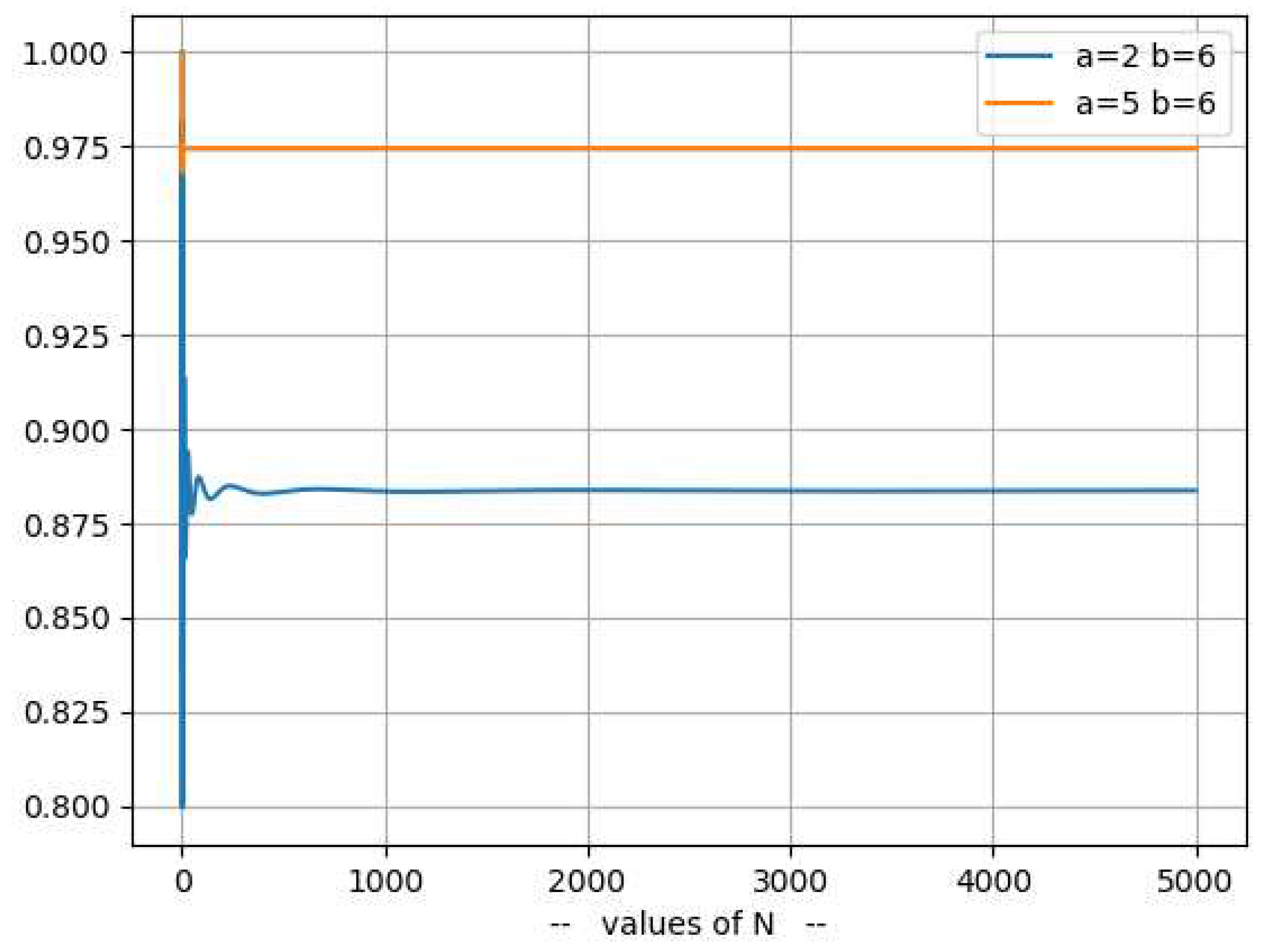
Figure 17. X z , n 2 for α>1.
Preprints 93993 g017
Figure 18. X z , n 2 for α<1.
Preprints 93993 g018
Figure 19. For a=0.5, b=ß1, X z , n 2 collapses to a line.
Preprints 93993 g019
Figure 20. X z , n 2 converges when n and α>1.
Preprints 93993 g020
Disclaimer/Publisher’s Note: The statements, opinions and data contained in all publications are solely those of the individual author(s) and contributor(s) and not of MDPI and/or the editor(s). MDPI and/or the editor(s) disclaim responsibility for any injury to people or property resulting from any ideas, methods, instructions or products referred to in the content.
Copyright: This open access article is published under a Creative Commons CC BY 4.0 license, which permit the free download, distribution, and reuse, provided that the author and preprint are cited in any reuse.
Prerpints.org logo

Preprints.org is a free preprint server supported by MDPI in Basel, Switzerland.

Subscribe

© 2024 MDPI (Basel, Switzerland) unless otherwise stated