Preprint
Article

Net Radiation Drives Evapotranspiration Dynamics in a Bottomland Hardwood Forest in the Southeastern United States: Insights from Multi-modeling Approaches

Altmetrics

Downloads

84

Views

15

Comments

0

A peer-reviewed article of this preprint also exists.

This version is not peer-reviewed

Submitted:

22 December 2023

Posted:

22 December 2023

You are already at the latest version

Alerts
Abstract
Evapotranspiration (ET) is a major component of water budget in Bottomland Hardwood Forests (BHF) and is driven by a complex intertwined suite of meteorological variables. The understanding of these interdependencies leading to seasonal variations in ET is crucial in better informing water resource management in the region. We used a structural equation modeling approach to analyze the drivers of ET using Eddy covariance water and heat flux data collected from a BHF, located in the Russel Sage Wildlife Management Area (RSWMA). It consists of mature closed-canopy deciduous hardwood trees with an average canopy height of 27 m. Factor analysis was used to characterize the shared variance among drivers and path analysis was used to quantify independent contributions of individual drivers. In our results, ET and net radiation (Rn) showed similar variability patterns with Vapor Pressure Deficit (VPD) and temperature in Spring, Summer, and Autumn seasons while they differ in Winter season. The path analysis shows that Rn has the strongest influence on ET variations via direct and indirect pathways. In the deciduous forests like BHFs, our results suggest ET is more energy-dependent during growing season (Spring and Summer) and early non-growing season (Autumn) while more temperature-dependent during winter season.
Keywords: 
Subject: Biology and Life Sciences  -   Forestry

1. Introduction

In the central and southeastern United States, deciduous forested wetlands located in broad floodplain areas bordering large river systems such as within the Lower Mississippi Alluvial Valley (LMAV) are referred to as Bottomland Hardwood Forests (BHFs) [1]. Many ecosystem services provided by BHFs, including water quality regulation, flood control, wildlife habitat, timber production, waste treatment and disturbance regulation, and climate moderation through carbon balance are of global importance [2,3]. Like other wetland types, a hydrological regime of alternating wet and dry cycles driven by fluctuating water levels of the associated rivers and groundwater level changes is characteristic of BHFs [4,5]. The sustainability of BHFs depends primarily on the longitudinal (upstream to downstream), lateral (river to floodplain to uplands and vice-versa), vertical (surface water to groundwater and vice versa), and temporal (seasonal and annual flooding) variability of water availability [6]. The primary force controlling the biota in BHFs is the flooding pulse from adjacent water sources which deposits dissolved nutrients, organic matter, and sediment, also contributing to the formation of young floodplains with each flooding pulse [7]. Even small changes in the duration and frequency of water levels can result in a distinct shift in the plant community as many species are adapted to a certain range of flood tolerance [8]. Therefore, a deeper understanding of the water use pattern and surface energy balance in these BHFs is crucial to preserving this dwindling ecosystem along the LMAV.
The study of BHF ecology remains incomplete without the assessment of factors that are integral to the proper functioning of these systems – evapotranspiration (ET), flood regimes, and precipitation. ET has been reported as a major component of BHF’s water balance in a number of studies along with LE (heat energy equivalent to ET) dominating the surface heat balance [9,10]. Several previous studies have identified biological and climatic drivers of bottomland hardwood ET using chrono sequence analysis [9], sap-flux measurements [11], and statistical modeling approaches [12] in the southeastern US. These studies report a strong correlation between net radiation (Rn), temperature, and other climatic conditions consistent with the site-specificities and variations in ET during different seasonal cycles. Vapor Pressure Deficit (VPD) has been established as one of the primary drivers of ET and is used increasingly in global simulation studies [13]. For example, [14] used maximum likelihood estimation methods to show a complex chain of correlations among ET, VPD, radiations, and temperature in northern high-latitude woodland ecosystems. The complex interrelationships among these atmospheric variables, which are essential for an assessment of the ultimate drivers of variations of ET can be explored using structural equation modeling (SEM). The use of SEM approach to diagnose the independent contributions of atmospheric drivers in determining the ET variability from the BHFs largely remains unexplored.
The complexity of interrelationships among multiple variables and their dependencies makes it challenging to quantify the actual contributions of the drivers of ET. SEM, a multivariate statistical modelling technique with factor analysis and path analysis, provides a framework to quantitatively evaluate these interrelationships that need to be untangled to characterize the role and independent contribution of each driver of the variations observed in ET. SEM analysis carried out with the data measured at multi-site high latitude regions showed that radiation, temperature, windspeed and relative humidity (RH) loaded heavily on the first factor during the warm season (May-September) [15,16]. Previous studies have applied path analysis to diagnose the drivers of ET in temperate [17], Arctic, and subarctic [15] regions, however, to our knowledge there is not a study reported on the water fluxes in the BHFs - where altered hydrologic cycle under global change scenarios, are critical and complex.
This paper is a comprehensive assessment of the drivers of variations in bottomland hardwood ET over hourly, daily, and weekly timescales across seasons. The main objectives were: (i) to characterize the interrelationships among variables driving ET over these timescales, and (ii) to characterize ET dependencies on various factors across different seasons. This study is unique to those mentioned above in various important ways. First, it utilizes SEM factor analysis and path analysis to provide a framework for quantitively evaluating the relative importance of drivers of ET variability in this system. Second, this is the first study of the drivers of ET in the BHF of Russel Sage Wildlife Management Area (RSWMA), a representative of floodplain forests in the entire LMAV. This study will fill the knowledge-gap in trying to understand the water flux dynamics from this region.

2. Methods

2.1. Study Site

This study was conducted at a BHF in the RSWMA (Figure 1) in Northeast Louisiana (32.46°N, -91.97°E; elevation 18 m ASL), managed by the Louisiana Department of Wildlife and Fisheries (LDWF). RSWMA is located within the Bayou Lafourche floodplain and is subjected to annual late winter (December-February) to early spring (March-May) flooding. It currently covers an area of 38,213 acres with mature hardwood stands that vary in age from 90-120 years (pers comm Larry Savage, LDWF).
The broadleaved deciduous forest canopy consists of co-dominant canopy species overcup oak (Quercus lyrate Walter) and water hickory (Carya aquatica (F. Michx.) Elliott), along with other canopy species such as green ash (Fraxinus pennsylvanica Marsh.), and sugarberry (Celtis laevigata Willd.) in the poorly drained soil [5]. In the first bottoms on low ridges, flats and sloughs, American elm (Ulmus americana L.), sweetgum (Liquidamber styraciflua), winged elm (Ulmus alata Michx.), and red maple (Acer rubrum L.) are abundant. In the newly formed sandbars on river margins, black willow (Salix nigra Marshall), cottonwood (Populus deltoides W. Bartram ex Marshall), river birch (Betula nigra L.), American sycamore (Platanus occidentalis L.) are prominent. The well-drained bottom ridges were dominated by sweetgum and water oak (Quercus nigra L.) characteristic species of BHF of the LMAV. The canopy is relatively flat with a mean tree height of 27 m. The LAI of the forested area, derived from Moderate Resolution Imaging Spectroradiometer (MODIS) instrument-based observations, was below 1 throughout the winter season, and on average reached a maximum of 6.53 in July. The soil type was Perry Clay, a fine-textured sediment that has low permeability and a moderate capacity to hold water [18].

2.2. Measurements of Above-Canopy Fluxes

Eddy Covariance (EC) technique was used to measure the amount of water vapor that was exchanged between the atmosphere and the BHF ecosystem. The wind components, sonic temperature, and gas concentrations were collected at 10 Hz frequency using an open-path IRGASON (Campbell Scientific Inc., USA). The EC system was mounted 12 m above the forest canopy and was directed towards the southwest, prevailing wind direction at the site and the fetch of the tower was 2 km.

2.3. Measurements of Meteorological, Phenological, and Hydrological Variables

Other measurements, relevant to land-plant-atmosphere interactions, were carried out from the tower to understand how they affect the hydro-dynamics at the study site. The meteorological measurements include air temperature, precipitation, wind speed and direction, barometric pressure, and RH. VPD was calculated as the difference between saturated and actual vapor pressures at the given temperature, based on the relative humidity and air temperature data. A net radiometer (NR-LITE2, Campbell Scientific Inc., USA) was used to measure the difference between the incoming and outgoing radiation at the site. A photosynthetically active radiation (PAR) sensor (LI190SB QUANTUM SENSOR, Campbell Scientific Inc., USA) was used to quantify the photosynthetic photon flux density (PPFD). Precipitation was measured by a tipping bucket rain gauge (TE525, Campbell Scientific Inc., USA).

2.4. Data Collection, Processing, and Gap-Filling Fluxes

All data were acquired using a solid-state data logger (CR3000, Campbell Scientific Inc., USA). The data were stored on a 2 GB CompactFlash card which was retrieved monthly. The raw flux data were grouped into individual 30-minute files and converted into TOA5 format before processing. These unprocessed data were screened for quality control and gap-filled using LoggerNet, EddyPro, TOVI, and REddyProc R packages [19]. To determine the periods of low mixing, which can lead to underestimation of water and heat fluxes, the frictional velocity (u*) threshold was identified using the Moving Point Test approach in TOVI [20]. Further quality control screening was carried out to filter potential data outside the u* threshold value (0.4 m/s).
Data recorded from 1 January 2014 to 31 December 2021 were used in this analysis. There was a major missing data gap due to instrument failure from January 2016 to July 2016, November 2018 to December 2020, and was not included in the analysis. Small gaps (<2 h) due to lower quality data were gap-filled using the Marginal Distribution Sampling Technique using the R package, REddyProc. Meteorological data from a nearby meteorological station (Monroe Airport – MLU) and NASA’s Prediction of Worldwide Energy Resources (POWER) [21] database were used for gap-filling temperature and precipitation data when necessary. The gap-filled data accounted for less than 20% of the whole EC data. The water losses associated with ET were quantified by the conversion of LE values from (W/m2) to mm/day [15]. To compare the means and assess the inter-relationships among variables, we performed an ANOVA test and the associated post-hoc tests, and SEM analysis as required, using R (v4.1.1, R Core Team 2023) [22].
The data was aggregated into hourly, daily and weekly datasets spanning the growing (March-August) and non-growing (September-February) seasons. Variables with more than 50% of its half-hourly data missing were not included in the SEM analysis. The missing data was then adjusted as described in [23] by dividing each daily and weekly values by the fraction of the data present for that particular unit of time. RH and soil moisture, two of the primary drivers of ET were not included in our analysis since RH is redundant to VPD, and soil moisture was not measured in our study.

2.5. Structural Equation Modelling (SEM)

As ET is influenced by a suite of atmospheric variables, a powerful multivariate analysis technique was required to identify those strongly driving the variation in the rate of ET. Different empirical approaches [9,11,12,24] and machine learning algorithms [25] have been in practice to characterize the key drivers of ET. However, due to the complexity of a large dataset with interdependent variables, SEM emerges as a suitable multivariate analysis technique to reduce the dimensionality and isolate common variance shared among variables from the residual variance unique to each variable [26]. Depending on the types of variables being modeled and their relationships with the predictor variables, several categories of models fall under the suite of SEM. A Factor analysis derives the latent constructs from variables that share the most variance with related variables while allowing them to be influenced by the seasonal cycles in the dataset, and the path analysis explains the structural pathways of the interrelationships among variables while testing for underlying causal mechanisms. Together, these analyses allow inferences to be made about the independent contributions of interrelated variables in the dataset.

2.6. Factor Analysis

Factor analysis estimates latent variables based on the correlated variations of the dataset (e.g., associations, causal relationships) and can reduce the dimensionality of the dataset, standardize the scale of multiple indicators, and account for the correlations inherent in the dataset [26]. The covariance matrix is central to the factor analysis, as described by the various equations in textbooks [26,27]. There are two types of factor analyses: Exploratory Factor Analysis (EFA) and Confirmatory Factor Analysis (CFA). In practice, EFA is often performed to select the useful underlying latent constructs for CFA when there is little prior knowledge about the latent construct [28]. The CFA is applied when the indicator for each latent variable is specified according to the related theories or prior knowledge. However, both types operate under the same basic assumption that “for a set of observed variables there are a suite of underlying factors which explain the interrelationships among the variables” [15]. The strongest association with ET is shown by variables that load highly on factors in which ET loads strongly as well.

2.7. Path Analysis

Path analysis helps to quantify the direct and indirect relationships among multiple variables while allowing them to covary with other variables in the dataset. It is very powerful in testing and developing the structural hypothesis where variables can influence an outcome directly and indirectly through another variable (e.g., mediation) [29]. This specific type of SEM uses a set of exogenous variables (variance is independent of other variables) to predict endogenous variables (variance is dependent on other variables) while allowing the variables to predict each other in the process [15]. We used R-Lavaan package (v4.1.1, R Core Team 2023) to define and run the model to predict ET using Rn, VPD, temperature, windspeed, and precipitation. The output yields regression estimates, standard errors, z-values, and p-values for each variable for that specific analysis. The path coefficients (regression coefficients) represent the slope of the linear relationship between the response variable and predictor variables independent of all other variables. The model was run on the hourly, daily, and weekly timescales for a sufficiently large sample size and model performance confidence. Additionally, the results from factor analysis were used to develop latent constructs, and a structural model was run to characterize the direct and indirect contributions of observed and latent variables in ET variability.
The statistical significance of differences among path coefficients were tested using ANOVA for hourly, daily, and weekly timescales. For the group of variables with significant results, TukeyHSD post hoc test was carried out to further examine the pairwise differences in path coefficients. Overall, using these analyses, we were able to categorize the variables/factors having similar variability patterns and quantify the independent contributions of each of those in influencing ET, as variables with large significant path coefficients can be interpreted to have a large influence on ET.

2.7. Akaike’s Information Criteria (AIC) and Model Selection

An information criterion approach (AIC) was also used to evaluate how well our models fit the data. AIC was used to develop candidate models with different combinations of potentially interacting variables that were also used in the SEM. By calculating and comparing the AIC scores of several candidate models, the model with the lowest AIC value and the highest AIC weight was selected as the best model using R-AICmodavg package.

3. Results

3.1. Factor Analysis

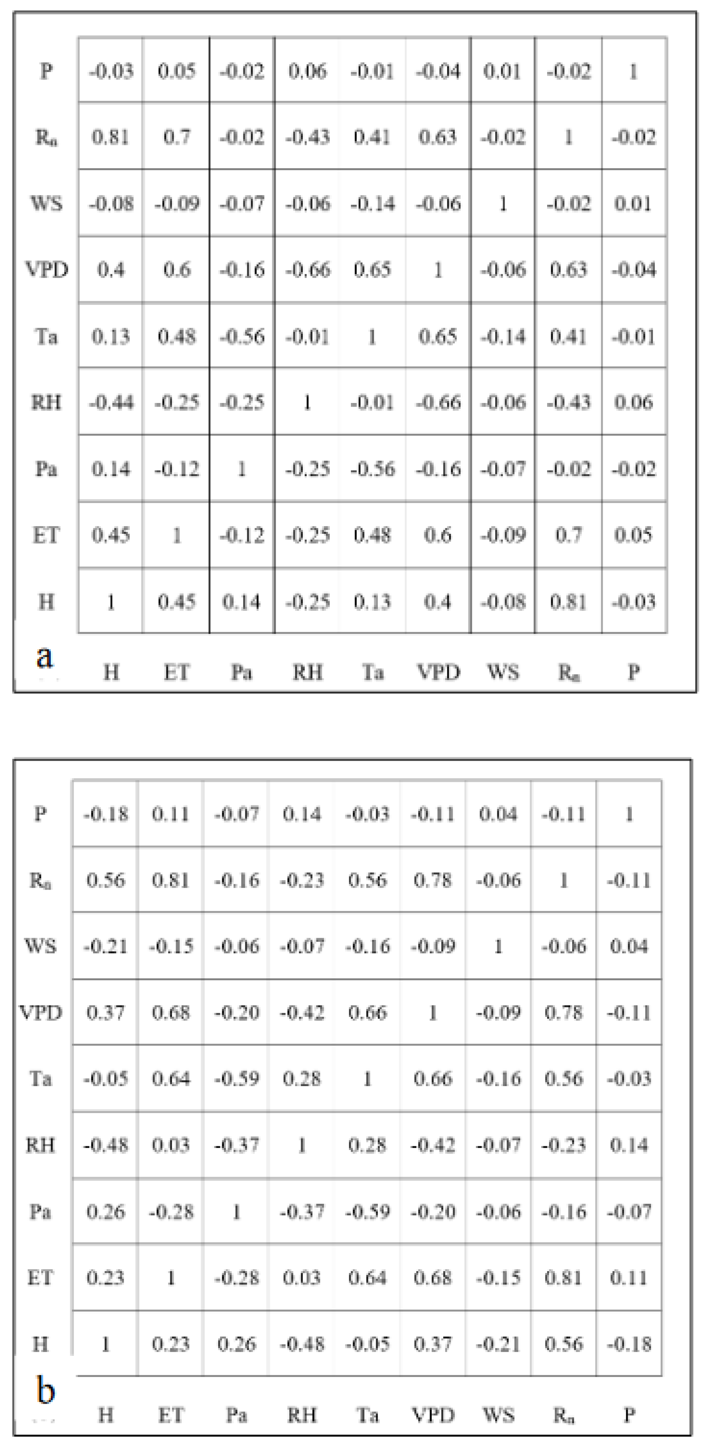
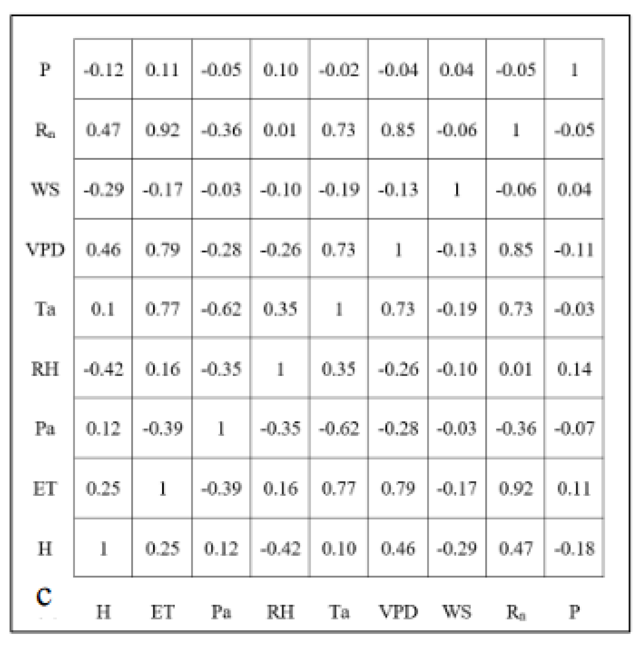
As a preliminary investigation of the relationships, Figure 2 shows the correlation matrix among all variables for all seasons at the hourly, daily, and weekly timescales. ET was highly correlated (| r | > 0.5) with Rn, VPD, sensible heat, and temperature at all timescales. Precipitation was weakly correlated to ET at all timescales with positively increasing coefficients at higher timescales. Interestingly, windspeed showed a weak negative correlation at hourly timescales with an increasing negative correlation at daily and weekly timescales. Rn was also highly correlated to sensible heat and VPD, with a moderate correlation to temperature. Further, temperature and VPD showed a strong correlation with increasing coefficients at larger timescales.
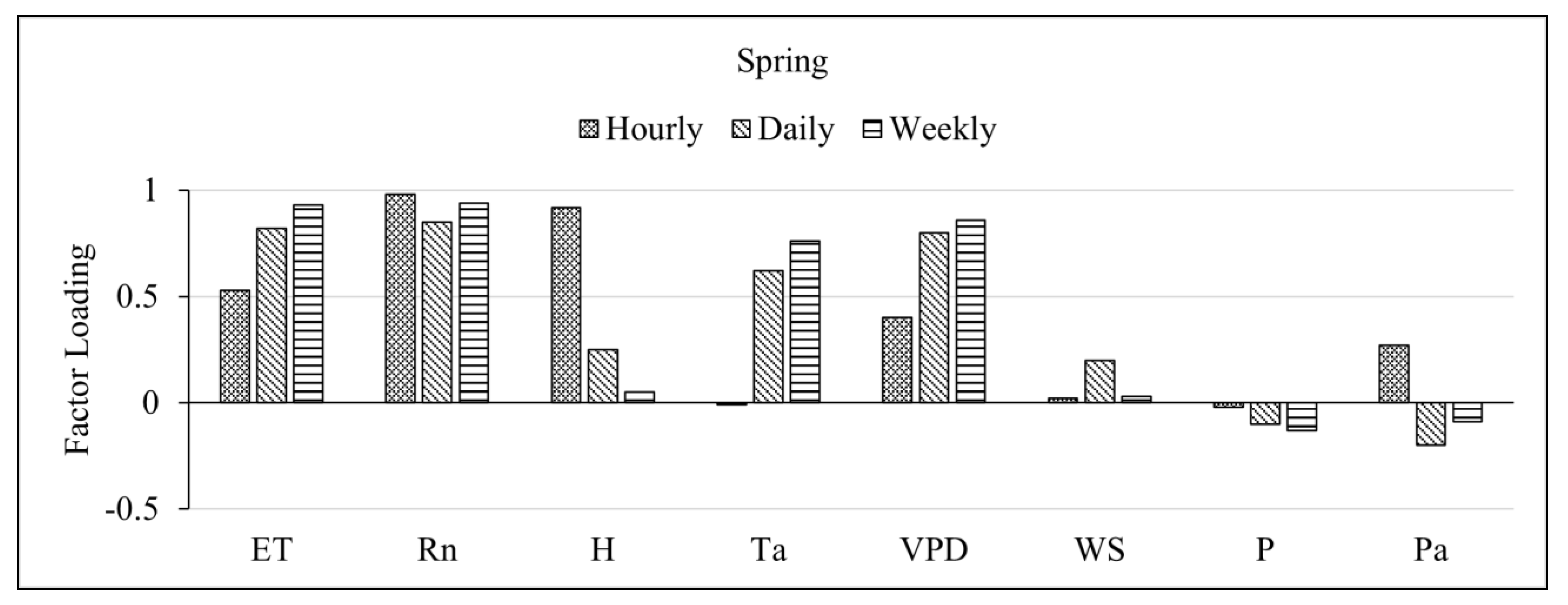
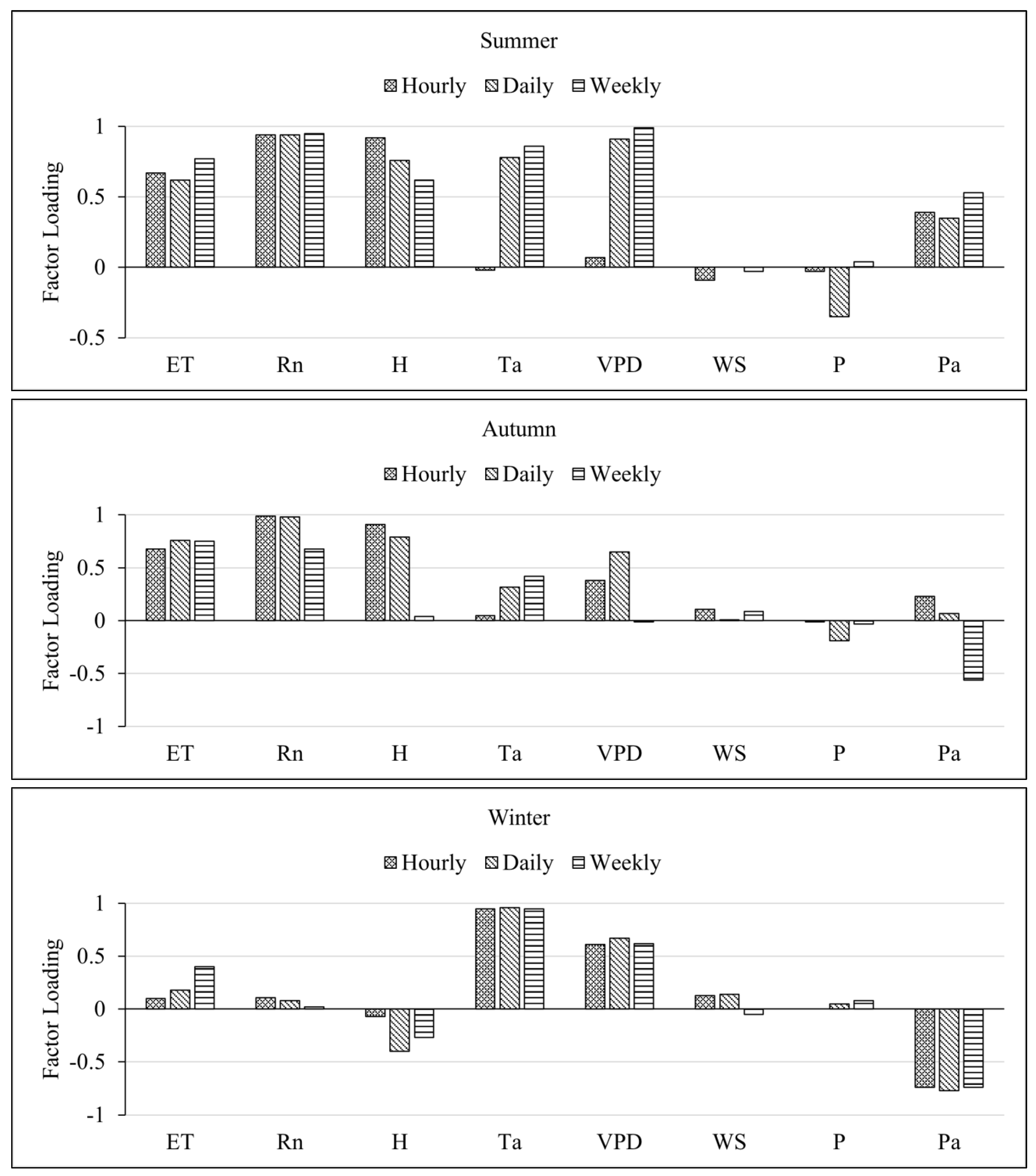
As evidenced by the correlation plots above, many of these variables share similar variability patterns and are strongly influenced by each other. This necessitated a method to quantify the independent contributions of each variable to the variability in ET. As described in Section 2.6, factor analysis was carried out across all seasons and variables shown above (excluding RH) to segregate them into groups showing similar variability patterns. The first factor loadings for these variables across different seasons are shown in Figure 3.
ET, Rn, sensible heat flux, temperature, and VPD all loaded highly positive on the first factor for all seasons except for the winter season where ET and Rn loaded comparatively lower than VPD and temperature. Also, sensible heat flux, and pressure loaded highly negatively in winter. Windspeed and rain (precipitation) showed low factor loadings which become highly variable as the timescale increases and seasons change.
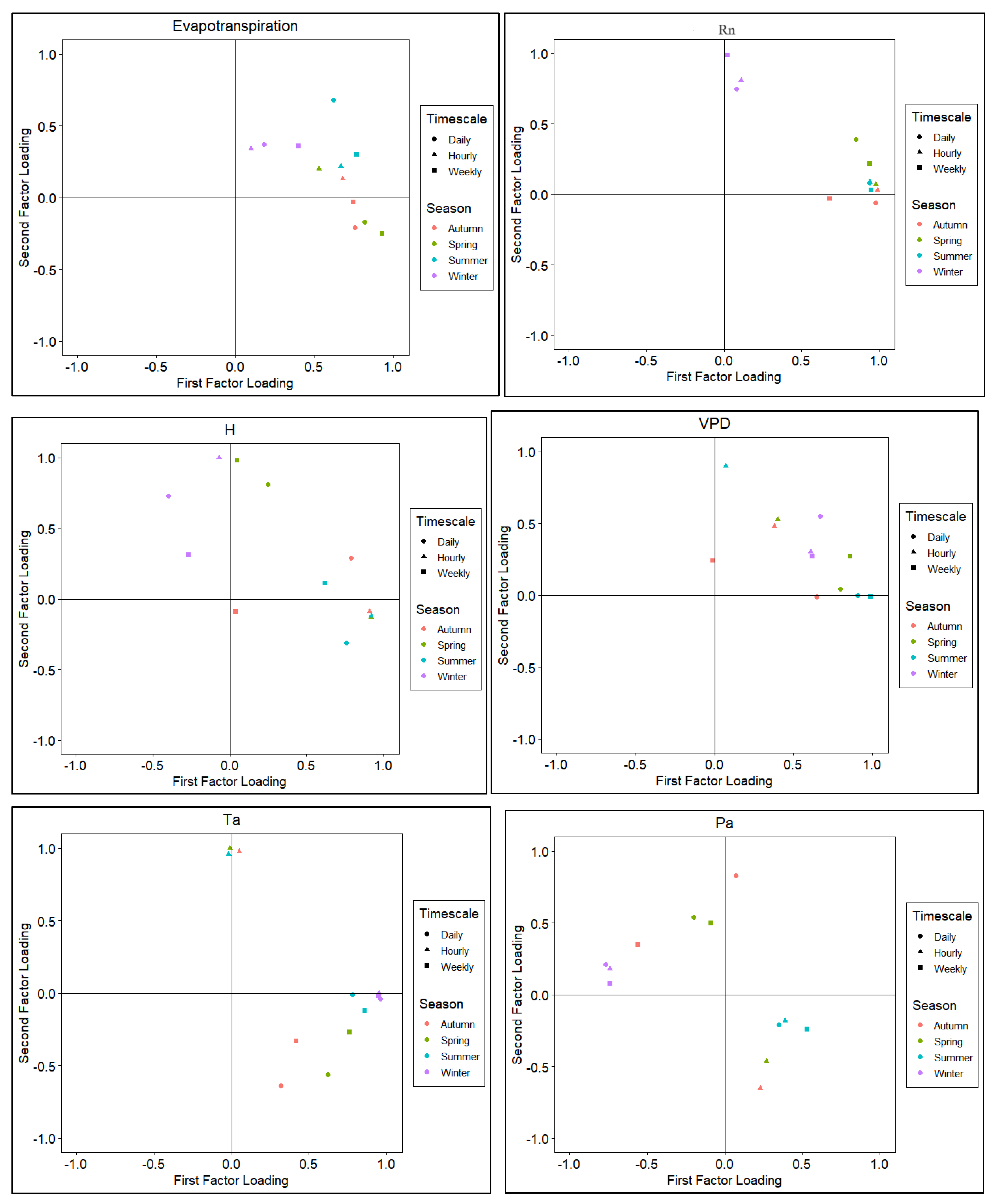
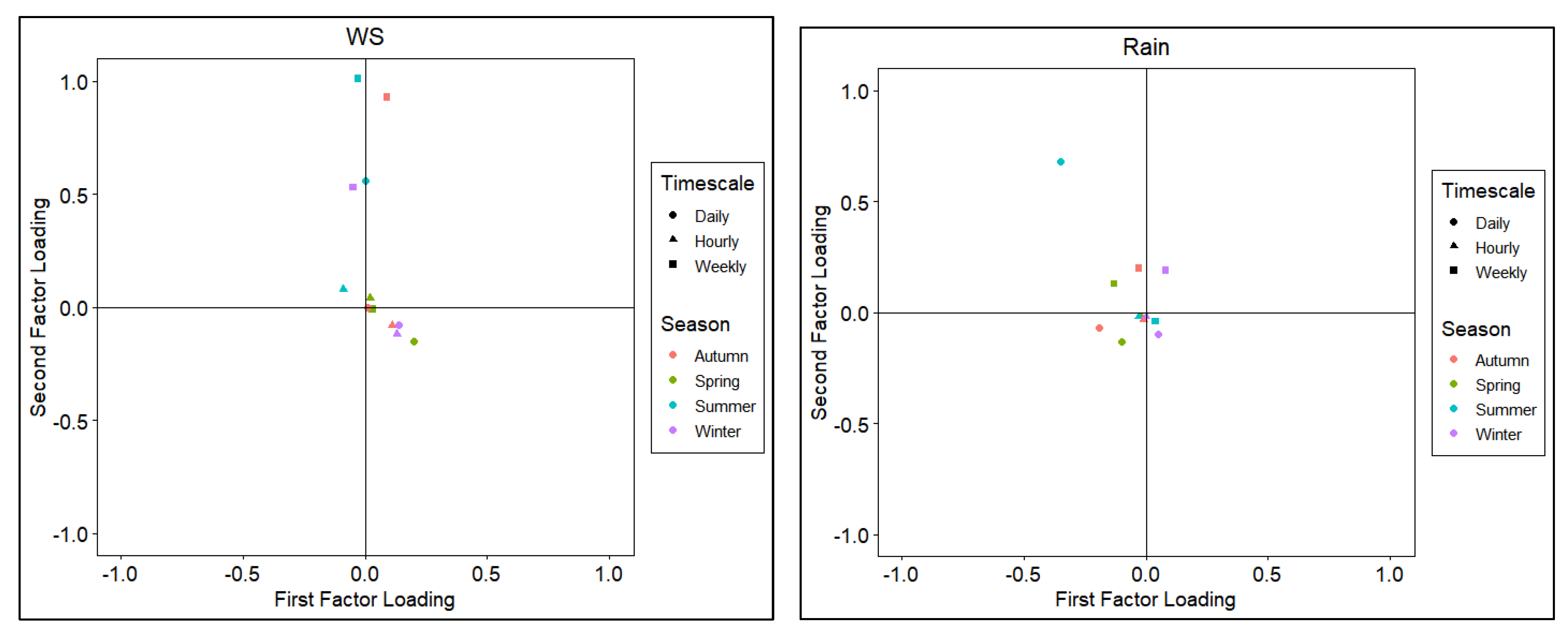
The factor analysis yielded multiple factor loadings with the first factor capturing approximately 60% of the variability in the dataset. The first and second factor loadings for all variables are shown in score plots in Figure 4 with groupings similar to that in Figure 3. Factor loading pairs were categorized by color for seasons and markers for timescales (hourly, daily, and weekly). Score plots revealed the spread of first and second factor loadings across seasons and timescales.
Consistent with Figure 3, ET, Rn, temperature, and VPD loaded highly on the first factor for all the seasons except for winter where second factor loadings are higher. For sensible heat flux and pressure, data were scattered on the plot can be seen while windspeed and rain had both loadings more clustered around the plot origin.

3.2. Path Analysis

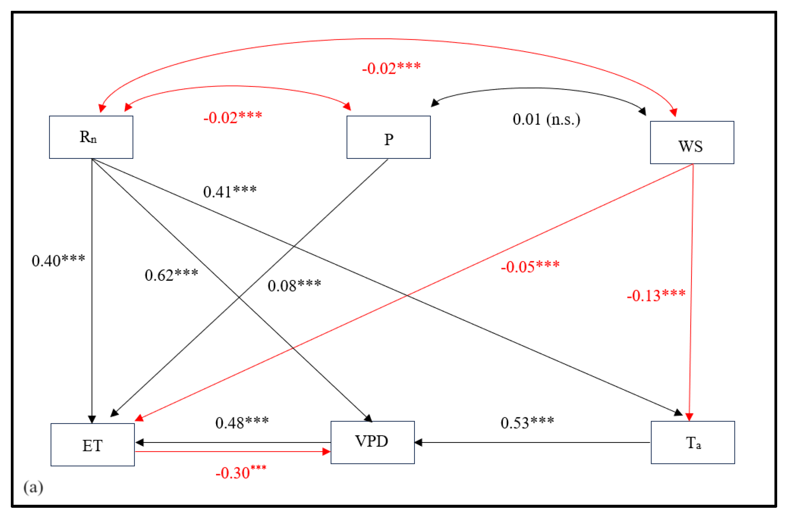
While the factor analysis helped to identify variables with similar variability patterns, the correlations deduced from this analysis alone do not represent the relative importance of one variable in determining ET variability, independent of the effect of other inter-related variables. Hence, a combination of path analysis with factor analysis is helpful to demonstrate the direct dependencies of ET on one variable independent of other variables, whereby regression coefficients represent the strength of independent contributions. The direct and indirect dependencies and associations between different variables in terms of physical pathways derived from the path analysis are shown in Figure 5. Sensible heat flux and pressure were not included in the analysis due to poor model fit.
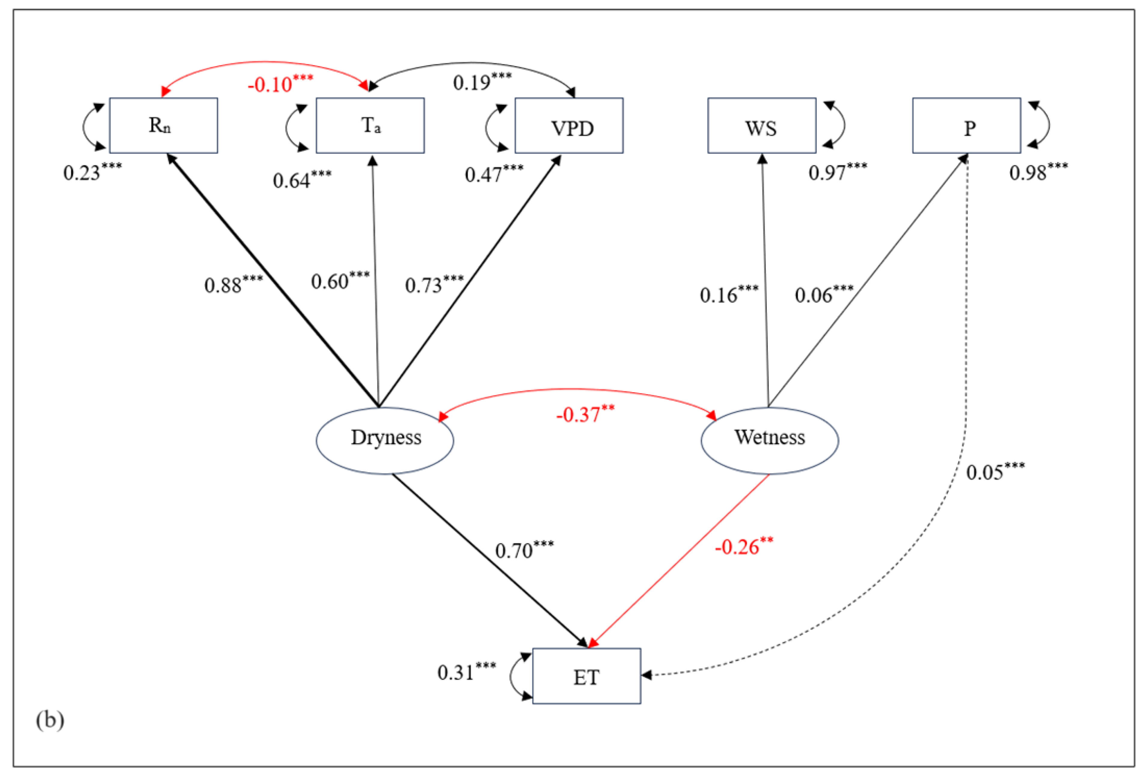
The standardized solutions for the best fit path model and structural model [χ2(df=4, N=42471)=752, p<0.0001], Comparative Fit Index (CFI) = 0.98, Tucker Lewis Index (TLI) = 0.96, RMSEA = 0.06, SRMR = 0.02) are shown in Figure 5a and 5b. While correlation and factor loading plots showed Rn having the strongest correlation and shared variability pattern with ET, its direct independent influence on ET was lower. Similarly, Rn not only had a comparable direct effect on ET but also a strong indirect effect via VPD and temperature. VPD showed a strong positive influence on ET while in reverse, ET had a strong negative impact on VPD. VPD showed the largest impact on ET at hourly timescales. Air temperature was strongly driven by Rn which then influenced VPD, ultimately affecting ET in the process. Windspeed had a negligible negative effect on ET while precipitation (rain) had a feeble positive impact on ET, although windspeed showed a negative impact on temperature, thereby affecting ET indirectly as well.
In the daily and weekly timescales, these regression coefficients generally increased for all the pathways. For example, the Rn emerged as a major direct influencer of ET while the strengths of indirect linkages through VPD and temperature also increased at larger timescale. The direct effect of rain on ET increased positively while that of windspeed decreased overall.
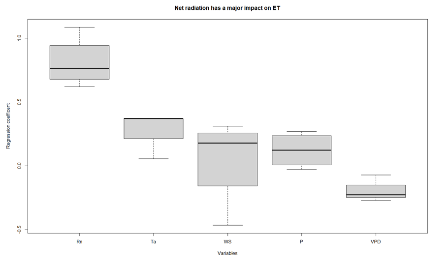
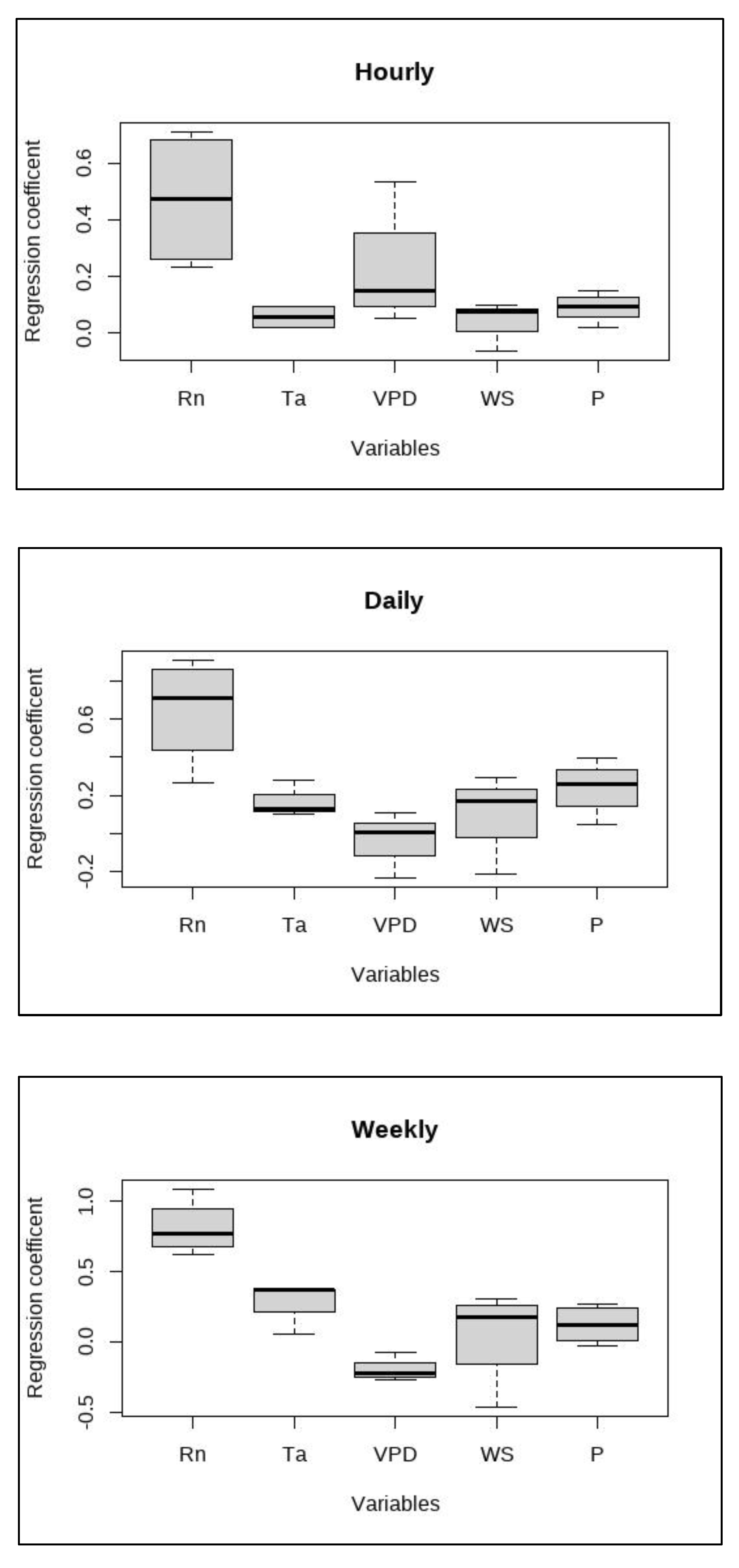
The combined results of path analysis with significant regression coefficients for different variables at hourly, daily, and weekly timescales are shown in Figure 6. Rn stood out with the highest median regression coefficient for all the timescales. VPD had the second highest independent contribution to ET variability on hourly scale while rain and temperature showed the same at daily and weekly timescales respectively. The windspeed showed lesser influence at hourly timescales while this increased for daily and weekly timescales. To test the significance of differences in the regression coefficients of different variables across these timescales, an ANOVA test was performed for all the categories. The results showed significant differences (p<0.05) in regression coefficients on all timescales for all variables. This was followed by a Tukey HSD post hoc analysis to test the significance for pairwise differences in regression coefficients. Only the regression coefficients for Rn showed significant differences with that of other variables. Thus, it was concluded that Rn is the major direct driver of ET variability in this ecosystem across all timescales.
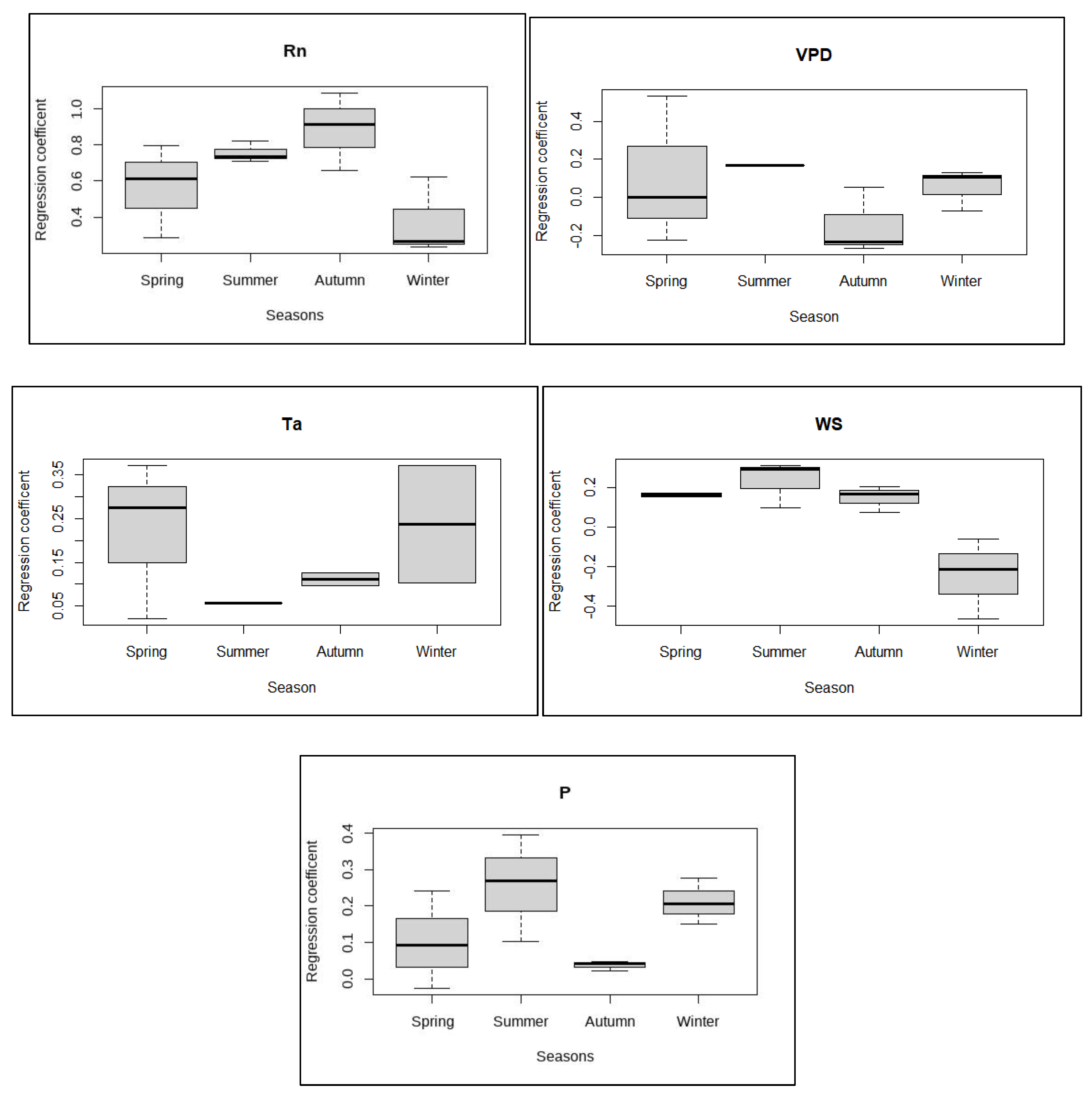
Similar to Figure 6, path analysis results were compared for all the variables with significant path coefficients across seasons. The distribution of path coefficients for each variable during Spring, Summer, Autumn, and Winter seasons are shown in Figure 7. Rn had the highest regression coefficient for Autumn season followed by Summer and Spring seasons. In Winter, the independent contribution of Rn was the lowest in determining the variability in ET. However, VPD showed the least contribution to ET variability in Autumn season which became maximum in the summer season. This revealed the VPD-dependent driving force in summer seasons when there is an abundant amount of water vapor in the atmosphere. The effect of temperature was observed greater during the spring and winter seasons compared to the summer and autumn seasons. Windspeed and rain had the highest impact during the summer season. The lesser effect of rain on ET variability during spring and autumn suggested sufficient water available for ET.

3.3. AIC results

Results of the AIC model selection suggested the model with ET as the dependent variable and Rn, VPD, temperature, windspeed, and precipitation independent variables, as the best fit model, given the data. All other models with possible combinations and meaningful interactions were tested and excluded based on the number of parameters (K>10). The best-fit model, carrying 98% of the cumulative model weight, included the above-mentioned variables with meaningful interaction effects (Table 1).
Results show that the best model was the interaction model (ET ~ Rn*Ta + VPD + WS*P), which corroborates with the findings from the SEM analysis. The “best” model carried 98% of the cumulative model weight and had the lowest AIC score. The next-best model was more than 2 AIC units higher than the best model (8.25 units) and carried only 2% of the cumulative model weight and was deemed unimportant since it did not meaningfully ‘add’ to the amount of information already explained by the best-fit model.

4. Discussion

The SEM approach has been used to diagnose drivers of ET using high-frequency data collected using the EC method for forested systems. The results of this study in a BHF at RSWMA revealed that the variability in ET is directly influenced by Rn during spring, summer, and autumn, primarily vegetatively active seasons. However, during times of vegetative dormancy (i.e., in winter) the variability in ET is largely influenced by VPD and temperature, indirect controls of Rn. These results are consistent with the strong seasonal cycle for the variables that gradually increase from winter to summer and gradually diminish from summer to winter. This typical seasonal cycle also suggests that the influence of temperature and VPD on ET is indirectly driven by Rn. The greater control of temperature and VPD as drivers of ET during winter is suggestive of the temperature-dependent ET, especially when the Rn-dependent direct control on ET is minimal. Hence, the direct as well as indirect (through strong control of Rn on temperature and VPD) control of Rn on ET across all seasons reinforces the role of Rn as a primary driver of ET in this forest.
The results from the best-fit model in AIC modeling support the inference from SEM that there’s an interaction between Rn and temperature. Furthermore, VPD showed independent influence as a predictor of ET than in interaction with Rn. This corroborates the increased influence of temperature on ET during vegetatively-dormant seasons as opposed to the higher impact of Rn on ET during vegetatively-active seasons. Although the independent, the positive impact of WS on ET has been previously established in many other studies [15,24], the interaction of WS with other variables like temperature and precipitation is likely to attenuate dryness (latent construct) and augment wetness, subsequently, regulating the rate of ET in this system. The best model from AIC suggested that these interactions are highly plausible and significant in determining the dynamics of ET in this BHF.
Consistent with the findings from the data collected in a BHF at RSWMA from 2014-2021, which showed Rn as the major direct and indirect driver of ET variability across different times of the year, the research at most other forest types have characterized Rn as a primary driver of ET. For example, [15] carried out SEM analysis in various boreal, tundra and permafrost ecosystems of high-latitude regions to demonstrate that Rn is the major driver of ET variability, albeit smaller independent contribution due to its control on other variables. On the contrary, a similar path analysis conducted in a mid-latitude agricultural site in northern China reported that Rn had the largest direct independent contribution on ET [17]. Brown [10] suggested that the increase in the amount of Rn received by the BHF in Missouri resulted in higher ET. Its vegetation composition, however, was silver maple (Acer saccharinum), Eastern cottonwood (Populus deltoides), Boxelder (Acer negundo), Sycamore (Platanus occidentalis) and are mostly different from those found around the US-ULM tower at RSWMA. Mackay [30] reported Rn as a major driver in upland hardwood growth forests whereas VPD as a major driver in wetland ecosystem during vegetatively active time of the year in Northern Wisconsin. The dominant hardwood vegetation composition at this site was sugar maple (Acer saccharum), basswood (Tilia americana L.), and green ash (Fraxinus pennsylvanica Marsh), mostly different from hardwood community found at RSWMA. However, a much higher effect of precipitation was reported in water-limited ecosystems as BHFs and seasonal cycles of canopy greenness in energy-limited ecosystems in higher latitudes using path analysis [31]. Similarly, in humid boreal regions, VPD and Rn were characterized as major drivers of sap-flow and thus transpiration during growing season as well as during drought [32].
In closed-canopy deciduous BHFs like the one in this study, Rn controls the variability of ET through two different pathways: first the direct pathway in which throughout the growing period (spring to summer) and early autumn, the Rn directly promotes the transpiration, which contributes about 80-90% of total ET as shown by [24]; second the indirect pathway in which when there are no leaves in vegetatively dormant period, the direct impact of Rn is somehow attenuated and the Rn influences ET variability indirectly via temperature and VPD. This is also supported by the consistent variability pattern shown by Rn and ET at diurnal and seasonal plots in Figure 5a b, and as reported by others [33,34].
Seasonally, albeit small, WS and precipitation play a critical role during summer when the atmospheric humidity is higher compared to other seasons. The increase in WS and precipitation positively influences wetness (one of the latent constructs), subsequently, affecting ET negatively in the process (path coefficients = 0.70 and -0.26 for dryness-ET and wetness-ET respectively). However, the negative effect of WS on ET as seen in Figure 5a could be due to its significant negative impact on temperature, which in turn has a strong influence on ET through VPD. As observed in the structural model in Figure 5b, WS contributes significantly as a major driver of atmospheric wetness, a latent construct with a significant negative effect on ET. In a study by Lobos-Roco [35] in the Atacama Desert ecosystem of Chile, it was shown that strong winds in the afternoon enhance mechanical turbulence and increase evaporation. A similar path analysis conducted in a mid-latitude agricultural site in China found similar results with WS having the least direct and indirect effects on ET [17]. On the other hand, precipitation has a minor positive impact as a driver of ET as seen in correlograms (Figure 2). However, the increasing negative impact of precipitation as seen in Figure 3 and its significant negative contribution to latent construct wetness, hence, ET over larger timescales is suggestive of reduction on ET as precipitation is observed for longer periods. From a similar research carried out at high latitude regions, Thunberg [15] reported similar control of precipitation as a driver of ET and suggested it as a potentially relevant driver of ET in mid-latitude regions such as these BHFs. These findings of seasonal relations of ET with meteorological variables are consistent with those from similar studies in Canadian forest ecosystems [36]. This also strengthens the conclusion that precipitation contributes positively to short-term enhancement in ET and negatively in the long run. These conclusions can be further strengthened by the simultaneous measurement of soil water content and heat flux on the site, one of the limitations of this study.
Since temperature and VPD are largely controlled by Rn, the importance of these variables as a driver of ET is more complex to understand, multifaceted, and largely dependent on the direct and indirect influence of the timing, duration, and intensity of solar energy in association with the seasonal phenological characteristics. The results from factor analysis suggested that their importance as a driver of ET becomes more prominent only during vegetatively dormant seasons when the direct control of Rn on ET remains lower. Rather these thermal variables share communality in their variability patterns and have a greater impact on ET by increasing the dryness (one of the latent constructs in the structural model) of the atmosphere as observed in Figure 5b. The ambient temperature not only positively influences VPD but also negatively impacts Rn. This could be due to lower retention of incoming radiation as the canopy gets heat saturated and higher loss of longwave radiation from the canopy as the temperature of the canopy increases. For example, with the increase in Rn before noon, all variables ET, temperature, and VPD increase consistently until the canopy gets saturated with heat, thus, leading to a decrease in Rn and ET after noon while the temperature and VPD increase further. This has implications for stomatal regulation of water loss, GPP, and canopy temperature regulation in this forested system as also suggested by [18]. The independent contributions of several other phenological and hydro-meteorological variables including temperature and VPD need to be further investigated to better understand the key role played by these variables as drivers of ET in this forested system.

5. Conclusion

During the study, the EC method was used to measure the water fluxes from 2014 to 2021 in the BHF at RSWMA in Northeast Louisiana. The results show that the Rn is a major direct driver of ET during the vegetatively active season and an indirect driver of ET via temperature and VPD during the vegetatively dormant season, implying a crucial role played by phenological changes in the process. The timing and duration of WS and precipitation play a significant role as drivers of ET in different seasons, albeit smaller independent contribution compared to other variables. This research needs to be expanded further to include other types of BHFs in the LMAV region to create a holistic understanding of water use patterns which can have implications for developing better-informed strategies for natural resource management in the whole region. This is even important in light of the findings of this research which suggest that unusual changes in weather patterns leading to unprecedented anomalies in temperature, VPD, and precipitation patterns could alter the water-use dynamics, exacerbating the deviations from the typical water cycle in this system. The advancement of machine learning and robust data analytical methods and their ability to process multiple variables simultaneously to disentangle the complex relationships among variables, has the potential to accomplish this goal, the results of which have implications for more accurate modeling and forecasting of water use dynamics for informed natural resource management in the region. In light of climate change, the ecosystem models studying the potential impact of unusual climatic conditions on the water fluxes can help better plan and prepare various mitigating efforts for the future of these temperate forests.

Institutional Review Board Statement

Not applicable.

Informed Consent Statement

Not applicable.

Data Availability Statement

Data will be made available through the AmeriFlux website.

Acknowledgments

This study was funded by the United States Geological Survey (USGS) [G21AC10226, 2021] awarded to JB. The authors acknowledge contributions by members of Plant Ecology Lab, University of Louisiana Monroe.

Conflicts of Interest

The authors declare no conflict of interest.

References

  1. King, S. L., and Keim, R. F. Hydrologic modifications challenge bottomland hardwood forest management. J. For. 2019, 117(5), 504-514. [CrossRef]
  2. Jenkins, W. A., Murray, B. C., Kramer, R. A., and Faulkner, S. P. Valuing ecosystem services from wetlands restoration in the Mississippi Alluvial Valley. Ecol. Econ. 2010, 69(5), 1051-1061. [CrossRef]
  3. Capon, S. J., Chambers, L. E., Mac Nally, R., Naiman, R. J., Davies, P., Marshall, N., and Williams, S. E. Riparian ecosystems in the 21st century: hotspots for climate change adaptation? Ecosyst. 2013, 16, 359-381.
  4. Wharton, C. H. The ecology of bottomland hardwood swamps of the Southeast: a community profile; U.S. Fish and Wildlife Service, Biological Services Program, Washington D.C., FWS/OBS-81/37, 1982; 133 pp.
  5. Reid, M. L. A Quarter Century of Plant Succession in a Bottomland Hardwood Forest in Northeastern Louisiana. MS Biology Thesis, University of Louisiana Monroe, Louisiana, 2014.
  6. Ward, J. V. The four-dimensional nature of lotic ecosystems. J. North Am. Benthol. Soc. 1989, 8(1), 2-8. [CrossRef]
  7. Hodges, J. D. Development and ecology of bottomland hardwood sites. For. Ecol. Manag. 1997, 90(2-3), 117-125. [CrossRef]
  8. Reid, M. L., Allen, S. R., and Bhattacharjee, J. Patterns of spatial distribution and seed dispersal among bottomland hardwood tree species. Castanea 2014, 79(4), 255-265. [CrossRef]
  9. Aguilos, M., Sun, G., Noormets, A., Domec, J.C., McNulty, S., Gavazzi, M., Minick, K., Mitra, B., Prajapati, P., Yang, Y. and King, J. Effects of land-use change and drought on decadal evapotranspiration and water balance of natural and managed forested wetlands along the southeastern US lower coastal plain. Agric. For. Meteorol. 2021, 303, p.108381. [CrossRef]
  10. Brown, K. Quantifying bottomland hardwood forest and agricultural grassland evapotranspiration in floodplain reaches of a mid-Missouri stream. MS Biology Thesis, University of Missouri-Columbia, Columbia, MO 65211, 2013.
  11. Meinzer, F. C., Woodruff, D. R., Eissenstat, D. M., Lin, H. S., Adams, T. S., and McCulloh, K. A. Above-and belowground controls on water use by trees of different wood types in an eastern US deciduous forest. Tree Physiol. 2013 33(4), 345-356. [CrossRef]
  12. Kassahun, Z., and Renninger, H. J. Effects of drought on water use of seven tree species from four genera growing in a bottomland hardwood forest. Agric. For. Meteorol. 2021, 301, 108353. [CrossRef]
  13. Fang, Y., and Leung, L. R. Relative controls of vapor pressure deficit and soil water stress on canopy conductance in global simulations by an Earth system model. Earth's Future 2022, 10(9), e2022EF002810. [CrossRef]
  14. Sabater, A.M., Ward, H.C., Hill, T.C., Gornall, J.L., Wade, T.J., Evans, J.G., Prieto-Blanco, A., Disney, M., Phoenix, G.K., Williams, M. and Huntley, B. Transpiration from subarctic deciduous woodlands: environmental controls and contribution to ecosystem evapotranspiration. Ecohydrology 2020, 13(3), p.e2190. [CrossRef]
  15. Thunberg, S. M., Euskirchen, E. S., Walsh, J. E., and Redilla, K. M. Diagnosis of atmospheric drivers of high-latitude evapotranspiration using structural equation modeling. Atmosphere 2021a, 12(10), 1359. [CrossRef]
  16. Thunberg, S. M., Walsh, J. E., Euskirchen, E. S., Redilla, K., and Rocha, A. V. Surface moisture budget of tundra and boreal ecosystems in Alaska: Variations and drivers. Polar Science 2021b, 29, 100685. [CrossRef]
  17. Zhang, B., Xu, D., Liu, Y., Li, F., Cai, J., and Du, L. Multi-scale evapotranspiration of summer maize and the controlling meteorological factors in north China. Agric. For. Meteorol. 2016 216, 1-12. [CrossRef]
  18. Bloch, Melissa B. Characterization of CO2 fluxes over Bottomland Hardwood Forests in Northeast Louisiana. MS Biology Thesis, University of Louisiana Monroe, Monroe, LA, 2021.
  19. Reichstein, M., Falge, E., Baldocchi, D., Papale, D., Aubinet, M., Berbigier, P., and Valentini, R. On the separation of net ecosystem exchange into assimilation and ecosystem respiration: review and improved algorithm. Glob. Change Biol. 2005 11(9), 1424-1439. [CrossRef]
  20. Papale, D., Reichstein, M., Aubinet, M., Canfora, E., Bernhofer, C., Kutsch, W., and Yakir, D. Towards a standardized processing of Net Ecosystem Exchange measured with eddy covariance technique: algorithms and uncertainty estimation. Biogeosciences 2006, 3(4), 571-583. [CrossRef]
  21. Prediction of Worldwide Energy Resource, National Aeronautics Space Administration (NASA), https://power.larc.nasa.gov/data-access-viewer (accessed on 15th June, 2021).
  22. RStudio Team (2023.09.0). RStudio: Integrated Development for R. RStudio, PBC, Boston, MA URL http://www.rstudio.com/.
  23. Lafleur, P.M., Humphreys, E.R., St. Louis, V.L., Myklebust, M.C., Papakyriakou, T., Poissant, L., Barker, J.D., Pilote, M. and Swystun, K.A. Variation in peak growing season net ecosystem production across the Canadian Arctic. Environ. Sci. Technol. 2012, 46(15), pp.7971-7977. [CrossRef]
  24. Bonan, G. Ecological climatology: concepts and applications, 3rd ed.; Cambridge University Press: University Printing House, Shaftesbury Road, Cambridge CB2 8BS, United Kingdom, 2016.
  25. Mosre, J., and Suárez, F. Actual evapotranspiration estimates in arid cold regions using machine learning algorithms with in situ and remote sensing data. Water 2021, 13(6), 870. [CrossRef]
  26. Bollen, K. Structural Equations with Latent Variables; John Wiley and Sons: New York, NY, USA, 1989; p. 709. ISBN 978-0-471-01171-2.
  27. Byrne, B. M. Structural equation modeling with Mplus: Basic concepts, applications, and programming; New York Press, NY: Routledge, USA, 2012.
  28. Gorsuch, R.L. Factor Analysis, 2nd ed.; Routledge Press: London, UK, 2014; p. 464. ISBN 9781138831995.
  29. Browne, M. W., and Cudeck, R. Alternative ways of assessing model fit. Sociol. Methods Res. 1992, 21(2), 230-258. [CrossRef]
  30. Mackay, D. S., Ewers, B. E., Cook, B. D., and Davis, K. J. Environmental drivers of evapotranspiration in a shrub wetland and an upland forest in northern Wisconsin. Water Resour. Res. 2007, 43(3). [CrossRef]
  31. Young, A.M., Friedl, M.A., Novick, K., Scott, R.L., Moon, M., Frolking, S., Li, X., Carrillo, C.M. and Richardson, A.D. Disentangling the Relative Drivers of Seasonal Evapotranspiration Across a Continental-Scale Aridity Gradient. J. Geophys. Res. 2022, 127(8), p.e2022JG006916. [CrossRef]
  32. Oogathoo, S., Houle, D., Duchesne, L. and Kneeshaw, D. Vapor pressure deficit and solar radiation are the major drivers of transpiration of balsam fir and black spruce tree species in humid boreal regions, even during a short-term drought. Agric. For. Meteorol. 2020, 291, p.108063. [CrossRef]
  33. Nazarbakhsh, M., Ireson, A. M., & Barr, A. G. Controls on evapotranspiration from jack pine forests in the Boreal Plains Ecozone. Hydrol. Process. 2020, 34(4), 927-940. [CrossRef]
  34. Ohta, T., Maximov, T.C., Dolman, A.J., Nakai, T., van der Molen, M.K., Kononov, A.V., Maximov, A.P., Hiyama, T., Iijima, Y., Moors, E.J. and Tanaka, H. Interannual variation of water balance and summer evapotranspiration in an eastern Siberian larch forest over a 7-year period (1998–2006). Agric. For. Meteorol. 2008, 148(12), pp.1941-1953. [CrossRef]
  35. Lobos-Roco, F., Hartogensis, O., Vilà-Guerau de Arellano, J., De La Fuente, A., Muñoz, R., Rutllant, J. and Suárez, F. Local evaporation controlled by regional atmospheric circulation in the Altiplano of the Atacama Desert. Atmospheric Chem. Phys. 2021, 21(11), pp.9125-9150. [CrossRef]
  36. Brümmer, C., Black, T.A., Jassal, R.S., Grant, N.J., Spittlehouse, D.L., Chen, B., Nesic, Z., Amiro, B.D., Arain, M.A., Barr, A.G. and Bourque, C.P.A. How climate and vegetation type influence evapotranspiration and water use efficiency in Canadian forest, peatland and grassland ecosystems. Agric. For. Meteorol. 2012, 153, pp.14-30. [CrossRef]
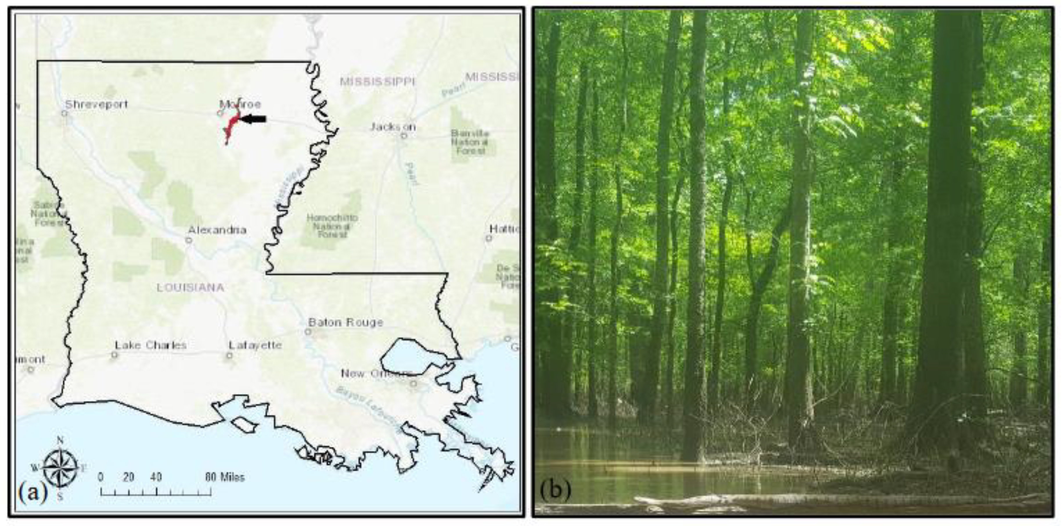
Figure 1. (a) Location map showing the study area Russel Sage Wildlife Management Area in Northeast Louisiana with the position of the US-ULM tower location indicated by the arrow tip, and (b) The study site shown flooded, as is typical during the late-winter and early-spring (Photo: JB).
Preprints 94154 g001
Figure 2. Correlation matrices among all variables for all seasons at the (a) hourly, (b) daily, and (c) weekly timescales.
Preprints 94154 g002aPreprints 94154 g002b
Figure 3. Factor loadings for Evapotranspiration (ET), Net radiation (Rn), Sensible heat flux (H), Temperature of air (Ta), Vapor Pressure Deficit (VPD), Windspeed (WS), Rain, and Pressure (Pa) on the first pattern of factor analysis for Spring, Summer, Autumn, and Winter seasons.
Preprints 94154 g003aPreprints 94154 g003b
Figure 4. Score plots of the first and second factor loadings by various timescales across different seasons. Variables include Evapotranspiration (ET), Net radiation (Rn), Sensible heat flux (H), Vapor Pressure Deficit (VPD), Temperature of air (Ta), Pressure (Pa), Windspeed (WS), and Precipitation (rain).
Preprints 94154 g004aPreprints 94154 g004b
Figure 5. The (a) path diagram and (b) SEM of all the observed variables (ET, Rn, Ta, VPD, WS and P) and latent constructs (Dryness and Wetness) within the path analysis with positive (black) and negative (red) path coefficients for hourly timescale across all seasons. Dashed line indicates direct contribution.
Preprints 94154 g005aPreprints 94154 g005b
Figure 6. Distributions of regression coefficients from all significant results of path analysis SEM at hourly, daily, and weekly timescales with sample size (n=12) for each variable. Black solid lines represent median values and boxes represent interquartile range.
Preprints 94154 g006
Figure 7. Distributions of regression coefficients from all significant results of path analysis SEM across different seasons with sample size (n=12) for each variable. Black solid lines represent median values and boxes represent interquartile range.
Preprints 94154 g007
Table 1. Results of AIC model selection with shortlisted candidate models with the number of parameters (K), Akaike’s Information Criteria (AIC), delta AIC, AIC weights, and log-likelihood (LL) values.
Model K AIC ΔAIC AIC weight LL
ET ~ Rn*Ta + VPD + WS*P 9 -104579 0 0.98 52298.53
ET ~ Rn*Ta + VPD + WS + P 8 -104570 8.25 0.02 52293.40
ET ~ Rn*Ta + VPD + WS 7 -104383 195.37 0 52198.84
ET ~ Rn*Ta + VPD
ET ~ Rn*VPD + Ta + WS*P
6
9
-104344
-99185
234.54
5393.08
0
0
52178.26
49601.99
Copyright: This open access article is published under a Creative Commons CC BY 4.0 license, which permit the free download, distribution, and reuse, provided that the author and preprint are cited in any reuse.
Prerpints.org logo

Preprints.org is a free preprint server supported by MDPI in Basel, Switzerland.

Subscribe

© 2024 MDPI (Basel, Switzerland) unless otherwise stated