Submitted:
22 December 2023
Posted:
22 December 2023
You are already at the latest version
Abstract
Keywords:
1. Introduction.
2. Methods
3. Results and Discussion
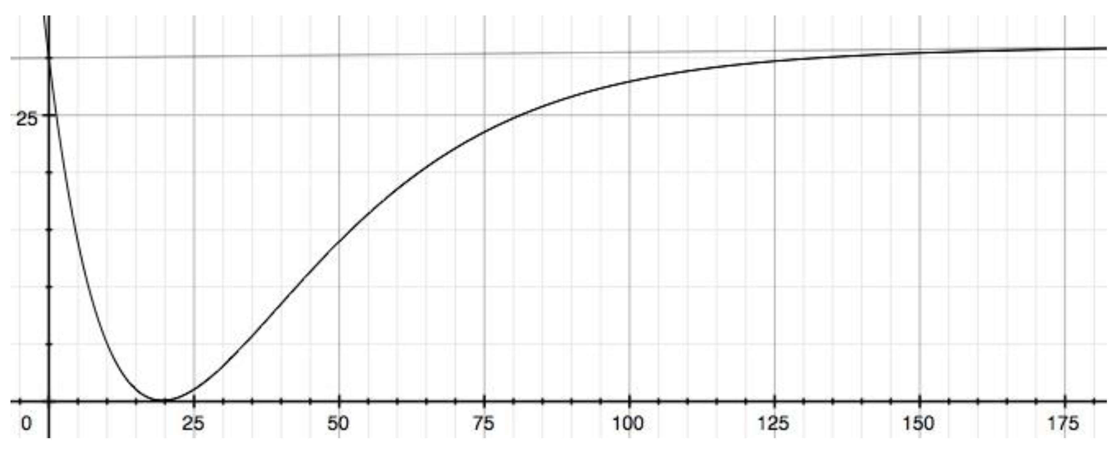
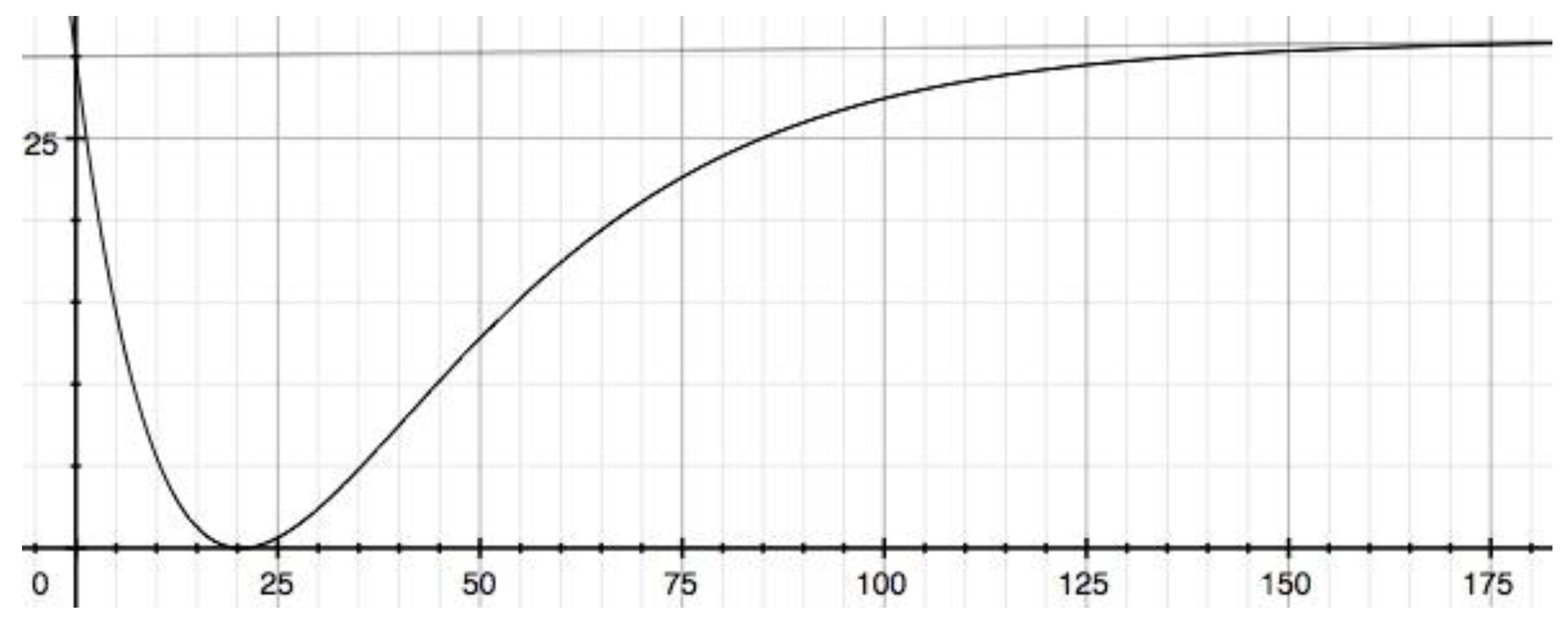
3.1. A sequential model reaction when the two rate constants are the same

3.2. Not ignoring the 0.5% increase from 0 mSv to 100 mSv

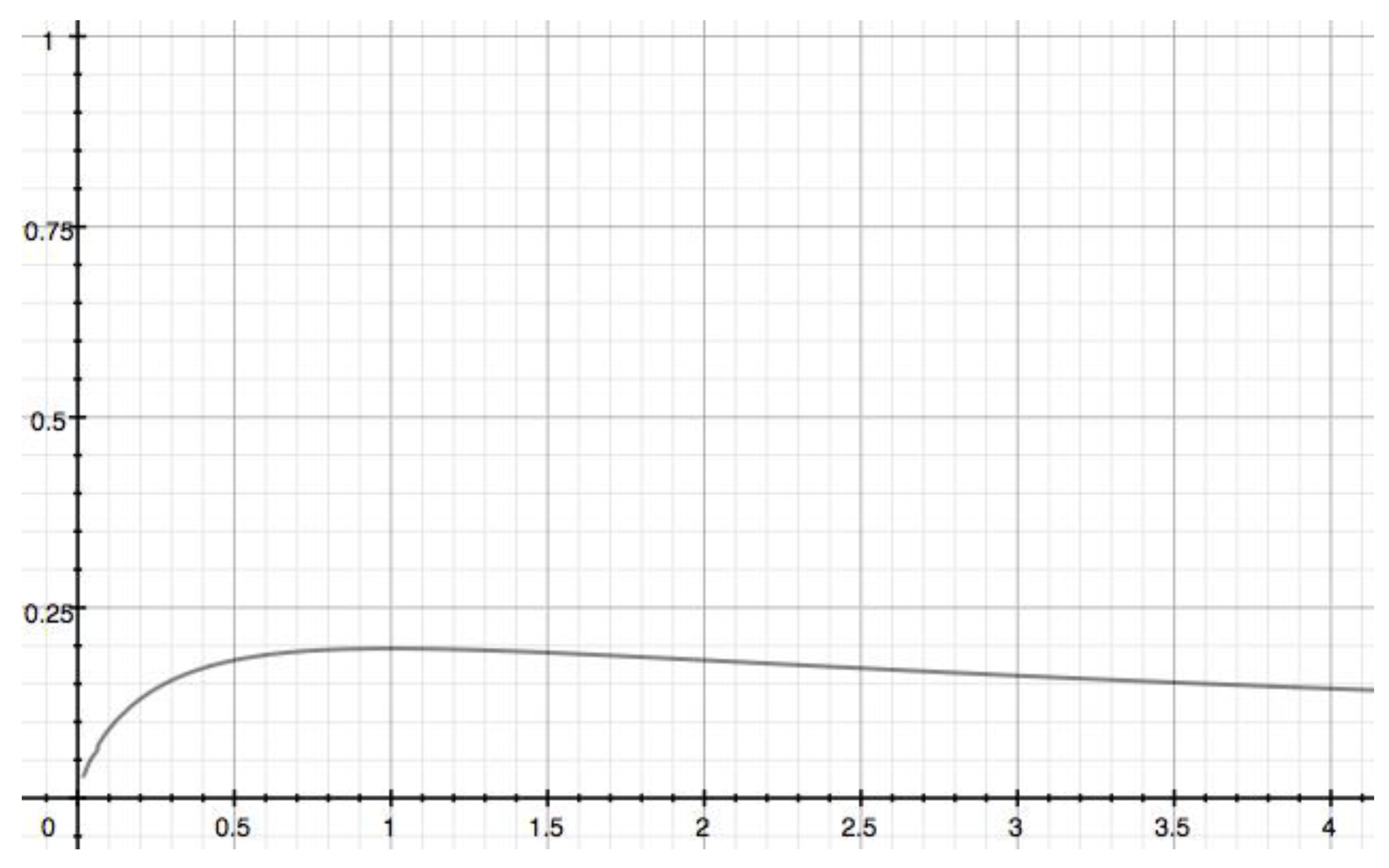
3.3. A sequential general model reaction when the two rate constants are different

4. Conclusion and Implications

Funding
Institutional Review Board Statement
Informed Consent Statement
Data Availability Statement
Acknowledgments
Conflicts of Interest
References
- Preston, D.L.; Ron, E.; Tokuoka, S.; Funamoto, S.; Nishi, N.; Soda, M.; Mabuchi, K.; Kodama, K. Solid cancer incidence in atomic bomb survivors: 1958–1998. Radiat. Res. 2007, 168, 1–64. [Google Scholar] [CrossRef] [PubMed]
- ICRP. Low-Dose Extrapolation of Radiation-Related Cancer Risk. ICRP Publication 99. International Commission on Radiological Protection; Elsevier Oxford: Amsterdam, The Netherlands, 2006. [Google Scholar]
- UNSCEAR. Summary of Low-Dose Radiation Effects on Health. UNSCEAR 2010 Report; United Nations Publications: New York, NY, USA, 2010. [Google Scholar]
- Tubiana, M.; Arengo, A.; Averbeck, D.; Masse, R. Low-dose risk assessment. Radiat. Res. 2007, 167, 742–744. [Google Scholar] [CrossRef] [PubMed]
- Mossman, K.L. Economic and policy considerations drive the LNT debate. Radiat. Res. 2008, 169, 245. [Google Scholar] [CrossRef] [PubMed]
- Leonard, B.E. Common sense about the linear no-threshold controversy-give the general public a break. Radiat. Res. 2008, 169, 245–246, Erratum in Radiat. Res. 2008, 169, 606. [Google Scholar] [CrossRef] [PubMed]
- Tubiana, M.; Aurengo, A.; Averbeck, D.; Masse, R. Low-dose risk assessment: The debate continues. Radiat. Res. 2008, 169, 246–247. [Google Scholar] [CrossRef]
- Feinendegen, L.E.; Paretzke, H.; Neumann, R.D. Two principal considerations are needed after low doses of ionizing radiation. Radiat. Res. 2008, 169, 247–248. [Google Scholar] [CrossRef] [PubMed]
- Mothersill, C.; Seymour, C. Low dose radiation mechanisms: The certainty of uncertainty. Mutat. Res. Genet. Toxicol. Environ. Mutagen. 2022, 876–877, 503451. [Google Scholar] [CrossRef]
- Boice, J.D.J. The linear nonthreshold (LNT) model as used in radiation protection: An NCRP update. Int. J. Radiat. Biol. 2017, 93, 1079–1092. [Google Scholar] [CrossRef]
- Olivieri, G.; Bodycote, J.; Wolff, S. Adaptive response of human lymphocytes to low concentrations of radioactive thymidine. Science 1984, 223, 594–597. [Google Scholar] [CrossRef]
- Wolff, S. The adaptive response in radiobiology: Evolving insights and implications. Environ. Health Perspect. 1998, 106 (Suppl. S1), 277–283. [Google Scholar]
- Azzam, E.I.; Raaphorst, G.P.; Mitchel, R.E. Radiation-induced adaptive response for protection against micronucleus formation and neoplastic transformation in C3H 10T1/2 mouse embryo cells. Radiat. Res. 1994, 138, S28–S31. [Google Scholar] [CrossRef] [PubMed]
- Shadley, J.D. Chromosomal adaptive response in human lymphocytes. Radiat. Res. 1994, 138, S9–S12. [Google Scholar] [CrossRef] [PubMed]
- Thierens, H.; Vral, A.; Barbé, M.; Meijlaers, M.; Baeyens, A.; Ridder, L.D. Chromosomal radiosensitivity study of temporary nuclear workers and the support of the adaptive response induced by occupational exposure. Int. J. Radiat. Biol. 2002, 78, 1117–1126. [Google Scholar] [CrossRef] [PubMed]
- Tapio, S.; Jacob, V. Radioadaptive response revisited. Radiat. Environ. Biophys. 2007, 46, 1–12. [Google Scholar] [CrossRef] [PubMed]
- Guéguen, Y.; Bontemps, A.; Ebrahimian, T.G. Adaptive responses to low doses of radiation or chemicals: Their cellular and molecular mechanisms. Cell Mol. Life Sci. 2019, 76, 1255–1273. [Google Scholar] [CrossRef] [PubMed]
- Devic, C.; Ferlazzo, M.L.; Foray, N. Influence of individual radiosensitivity on the adaptive response phenomenon: Toward a mechanistic explanation based on the nucleo-shuttling of atm protein. Dose-Response 2018, 16, 1559325818789836. [Google Scholar] [CrossRef]
- Agathokleous, E.; Calabrese, E.J.; Barcelo, D. Environmental hormesis: new developments. Sci. Total Environ. 2024, 906, 167450. [Google Scholar] [CrossRef] [PubMed]
- Socol, Y.; Dobrzynski, L.; Doss, M.; Feinendegen, L.E.; Janiak, M.K.; Miller, M.L.; Sanders, C.L.; Scott, B.R.; Ulsh, B.; Vaiserman, A. Commentary: Ethical issues of current health-protection policies on low-dose ionizing radiation. Dose Response 2014, 12, 342–348. [Google Scholar] [CrossRef]
- Luckey, T.D. Radiation Hormesis; CRC Press: Boca Raton, FL, USA, 1991. [Google Scholar]
- Sanders, C.L. Radiation Hormesis and the Linear-No-Threshold Assumption; Springer: Berlin, Germany, 2010. [Google Scholar]
- Feinendegen, L.E.; Bond, V.P.; Sondhaus, C.A. The dual response to low-dose irradiation: induction vs. prevention of DNA damage. In: Yamada, T.; Mothersill, C.; Michael, B.D.; Potten, C.S. Biological effects of low dose radiation. Excerpta Medica. International Congress Series 1211. Elsevier: Amsterdam, The Netherlands, 2000; pp. 3–17. [Google Scholar]
- Sutou, S. A message to Fukushima: nothing to fear but fear itself. Genes Environ. 2016, 38, 12. [Google Scholar] [CrossRef]
- Sutou, S. The 10th anniversary of the publication of genes and environment: memoir of establishing the Japanese environmental mutagen society and a proposal for a new collaborative study on mutagenic hormesis. Genes Environ. 2017, 39, 9. [Google Scholar] [CrossRef]
- Sutou, S. Low-dose radiation from A-bombs elongated lifespan and reduced cancer mortality relative to un-irradiated individuals. Genes Environ. 2018, 40, 26. [Google Scholar] [CrossRef] [PubMed]
- Sutou, S.; Koeda, A.; Komatsu, K.; Shiragiku, T.; Seki, H.; Yamakage, K.; Niitsuma, T.; Kudo, T.; Wakata, A. Collaborative study of thresholds for mutagens: proposal of a typical protocol for detection of hormetic responses in cytotoxicity tests. Genes Environ. 2018, 40, 20. [Google Scholar] [CrossRef] [PubMed]
- Rattan, S.I.S.; Bourg, E.L. Hormesis in health and disease.; CRC Press, Inc.: Boca Raton, USA, 2014. [Google Scholar]
- UNSCEAR. Sources and Effects of Ionizing Radiation. United Nations Scientific Committee on the Effects of Atomic Radiation. UNSCEAR 2000 Report; United Nations Publications: New York, NY, USA, 2000. [Google Scholar]
- NCRP. Evaluation of the Linear-Nonthreshold Dose-Response Model for Ionizing Radiation; NCRP Report No. 136; National Council on Radiation Protection and Measurements: Bethesda, MD, USA, 2001. [Google Scholar]
- Uchinomiya, K.; Yoshida, K.; Kondo, M.; Tomita, M.; Iwasaki, T. A mathematical model for stem cell competition to maintain a cell pool injured by radiation. Radiat. Res. 2020, 194, 379–389. [Google Scholar] [CrossRef]
- Kim, S.B.; Sanders, N. Model averaging with AIC weights for hypothesis testing of hormesis at low doses. Dose Response 2017, 15, 1559325817715314. [Google Scholar] [CrossRef] [PubMed]
- Kim, S.B.; Bartell, S.M.; Gillen, D.L. Inference for the existence of hormetic dose-response relationships in toxicology studies. Biostatistics 2016, 17, 523–536. [Google Scholar] [CrossRef] [PubMed]
- Esposito, G.; Campa, A.; Pinto, M.; Simone, G.; Tabocchini, M.A.; Belli, M. Adaptive response: Modelling and experimental studies. Radiat. Prot. Dosim. 2011, 143, 320–324. [Google Scholar] [CrossRef] [PubMed]
- Wodarz, D.; Sorace, R.; Komarova, N.L. Dynamics of cellular responses to radiation. PLoS Comput. Biol. 2014, 10, e1003513. [Google Scholar] [CrossRef]
- Socol, Y.; Shaki, Y.Y.; Dobrzyński, L. Damped-oscillator model of adaptive response and its consequences. Int. J. Low Rad. 2020, 11, 186–206. [Google Scholar] [CrossRef]
- Smirnova, O.A.; Yonezawa, M. Radioprotection effect of low level preirradiation on mammals: Modeling and experimental investigations. Health Phys. 2003, 85, 150–158. [Google Scholar] [CrossRef]
- Kino, K. The prospective mathematical idea satisfying both radiation hormesis under low radiation doses and linear non-threshold theory under high radiation doses. Gene Environ. 2020, 42, 4. [Google Scholar] [CrossRef]
- Kino, K.; Ohshima, T.; Takeuchi, H.; Kobayashi, T.; Kawada, T.; Morikawa, M.; Miyazawa, H. Considering existing factors that may cause radiation hormesis at <100 mSv and obey the linear no-threshold theory at ≥100 mSv. Challenges 2021, 12, 33. [Google Scholar] [CrossRef]
- Kino, K. The radiation-specific components generated in the second step of sequential reactions have a mountain-shaped function. Toxics 2023, 11, 301. [Google Scholar] [CrossRef] [PubMed]
- Calabrese, E.J.; Shamoun, D.Y.; Hanekamp, J.C. Cancer risk assessment: Optimizing human health through linear dose-response models. Food Chem. Toxicol. 2015, 81, 137–140. [Google Scholar] [CrossRef] [PubMed]
- Lampe, N.; Breton, V.; Sarramia, D.; Sime-Ngando, T.; Biron, D.G. Understanding low radiation background biology through controlled evolution experiments. Evol. Appl. 2017, 10, 658–666. [Google Scholar] [CrossRef] [PubMed]
- Scott, B.R. Residential radon appears to prevent lung cancer. Dose Response 2011, 9, 444–464. [Google Scholar] [CrossRef] [PubMed]
- Ministry of the Environment, Japan. Uniform basic information on health effects of radiation, etc. 2016 edition ver.2017001. Available online: https://www.env.go.jp/chemi/rhm/h28kisoshiryo/h28kiso-03-07-03.html (accessed on 13 December 2023).
- ICRP. The 2007 Recommendations of the International Commission on Radiological Protection. ICRP Publication 103.; Elsevier Oxford: Amsterdam, The Netherlands, 2007. [Google Scholar]
- Feinendegen, L.E. Evidence for beneficial low level radiation effects and radiation hormesis. Br. J. Radiol. 2005, 78, 3–7. [Google Scholar] [CrossRef] [PubMed]
- Feinendegen, L.E. Low doses of ionizing radiation: Relationship between biological benefit and damage induction. A synopsis. World J. Nucl. Med. 2005, 4, 21–34. [Google Scholar]
- Agathokleous, E.; Kitao, M.; Calabrese, E.J. Environmental hormesis and its fundamental biological basis: Rewriting the history of toxicology. Environ. Res. 2018, 165, 274–278. [Google Scholar] [CrossRef] [PubMed]
- Sadowska-Bartosz, I.; Bartosz, G. Antioxidant defense of Deinococcus radiodurans: how does it contribute to extreme radiation resistance? Int. J. Radiat. Biol. 2023, 99, 1803–1829. [Google Scholar] [CrossRef]
- Ranawat, P.; Rawat, S. Radiation resistance in thermophiles: mechanisms and applications. World J. Microbiol. Biotechnol. 2017, 33, 112. [Google Scholar] [CrossRef]
- Kasianchuk, N.; Rzymski, P.; Kaczmarek, Ł. The biomedical potential of tardigrade proteins: A review. Biomed Pharmacother. 2023, 158, 114063. [Google Scholar] [CrossRef] [PubMed]


Disclaimer/Publisher’s Note: The statements, opinions and data contained in all publications are solely those of the individual author(s) and contributor(s) and not of MDPI and/or the editor(s). MDPI and/or the editor(s) disclaim responsibility for any injury to people or property resulting from any ideas, methods, instructions or products referred to in the content. |
© 2023 by the authors. Licensee MDPI, Basel, Switzerland. This article is an open access article distributed under the terms and conditions of the Creative Commons Attribution (CC BY) license (http://creativecommons.org/licenses/by/4.0/).


