1. Introduction
Infrared spectroscopy technology [
1,
2,
3] is a technique for detecting the molecular structure and chemical composition of substances. This technology utilizes the energy level transition of molecules in substances under infrared radiation to measure the wavelength and intensity of absorbed or emitted light, producing specific spectrogram, which are used to analyze and judge the chemical bonds and structures of substances. This technology has important research applications in environmental monitoring [
4], garbage classification [
5], and life chemistry [
6]. Fourier Transform Infrared Spectrometer (FTIR) [
7,
8,
9] is an important means of measuring infrared spectra. It obtains interferogram through an interferometer and restores the interferogram to spectrogram based on Fourier transform. Passive FTIR is commonly used for the detection of atmospheric pollutants. It has the ability to collect data from any direction, allowing for all-weather, continuous, long-distance, real-time monitoring and rapid analysis of targets.
The classification characteristics of aeroengines are often related to fuel type, combustion method, and emission characteristics. Different types of aeroengines produce different gas components and emissions during the combustion process. The vibration and rotation of these molecules form specific infrared absorption and emission spectra. By analyzing the infrared spectra of aeroengine hot jet, the characteristics of the gas components and emissions produced by aeroengine combustion can be obtained. After a large number of hot jet infrared spectra are analyzed, a spectral feature library will be established, then the types of aeroengines is going to be determined, so that the identification of aeroengines will be realized.
In this paper, an algorithm for the classification and recognition of aeroengines is proposed, which combines the infrared spectrum feature vectors of aeroengine hot jet with the current popular classifier. The classifier includes supervised learning method SVM, integrated learning methods XGBoost, CatBoost, AdaBoost, Random Forest, LightGBM and Neural Network method. Accuracy, precision, recall, F1 value and confusion matrix as classification evaluation criteria. After many experiments, the accuracy of the classification of aeroengines has reached 98%.
The main contributions of this paper are as follows:
1. The infrared spectrum detection method for aeroengine hot jet is used as the basis and data source input of the identification of aeroengines. Aeroengine hot jet is an important infrared radiation characteristic of aeroengine, and the infrared spectrum provides the characteristic information of substances at the molecular level, so it is more scientific to use this method for classification.
2. FTIR is used to measure the infrared spectrum information of aeroengine hot jet. FTIR has the advantages of fast scanning speed, high resolution, wide measurement spectral range and high measurement accuracy. It can achieve fine spectral measurement, which is of great significance for the non-contact classification and recognition of aeroengines.
The architecture of this paper is as follows:
Section 1 describes the infrared spectroscopy technology, this paper uses the classification method, innovation and article architecture; In
Section 2, the spectral components of the hot jet are analyzed, and the construction method of spectral feature vectors are proposed;
Section 3 introduces seven mainstream classifier methods;
Section 4 describes the experimental content, including the experimental design of aeroengine spectrum acquisition, data set production and spectral feature vectors extraction, and the accuracy evaluation of classification prediction results;
Section 5 summarizes the paper and puts forward the idea of the next research direction.
2. Spectral Feature Analysis and Spectral Feature Vector Construction
In this section, the Brilliant Temperature Spectrum(BTS) and components of aeroengine hot jet are analyzed, and a method of constructing spectral feature vectors based on CO2 characteristic peaks is proposed.
When passive FTIR is used in gas detection and identification studies, the method of calculating the BTS with a constant baseline can be utilized due to the high emissivity of most of the substances in nature that serve as the background. The Brilliant Temperature [
10,
11] of an actual object is equivalent to the temperature of a blackbody at the same wavelength, when the intensity of the spectral radiation of the actual object and the blackbody are equal. It is based on equal brightness and is used to characterize the actual object's own radiation. The use of BTS does not require pre-measurement of the background spectrum and enables the target gas characteristics to be extracted directly from the BTS analysis.
In order to obtain the BTS from the passive infrared spectrum, it is necessary to first deduct the spectral signal measured by the spectrometer from the bias and response of the instrument to obtain the spectral radiance spectrum entering the spectrometer, and from the radiance spectrum obtained, the equivalent temperature of the radiance spectrum
T(
v) can be calculated according to Planck's law of radiation by transforming Planck's formula to obtain the following formula:
where h is Planck's constant with a value of 6.625*1023J·S, c is the speed of light with a value of 2.998*108 m/s, v is the wave number in cm-1, and k is Boltzmann's constant with a value of 1.380649×10⁻²³J/K, L(v) is the radiance about the wave number.
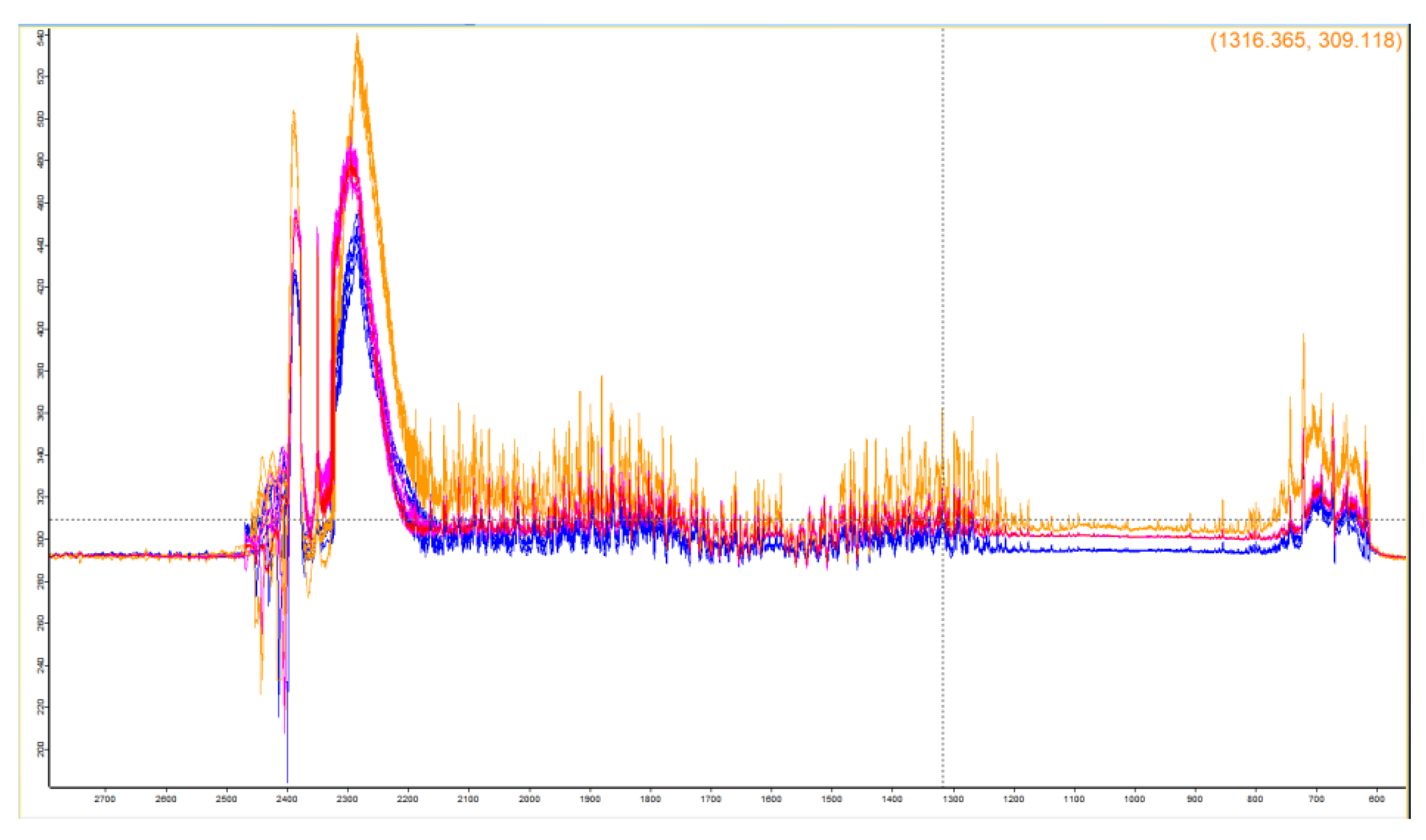
The experimentally measured infrared spectra of aeroengine hot jets of three turbojet engines are shown in
Figure 1, where the horizontal coordinates are the wave numbers and the vertical coordinates are the BTS.
The emission products of aeroengine mainly include oxygen (O
2), nitrogen (N
2), carbon dioxide (CO
2), steam (H
2O), carbon monoxide (CO) et al. The combustion products are mainly divided into: ① Air composition not participating in combustion, including O
2 and N
2; ② Products of combustion reactions, mainly NO
x; ③ The end product of an ideal combustion process, including CO
2, H
2O and CO [
12].
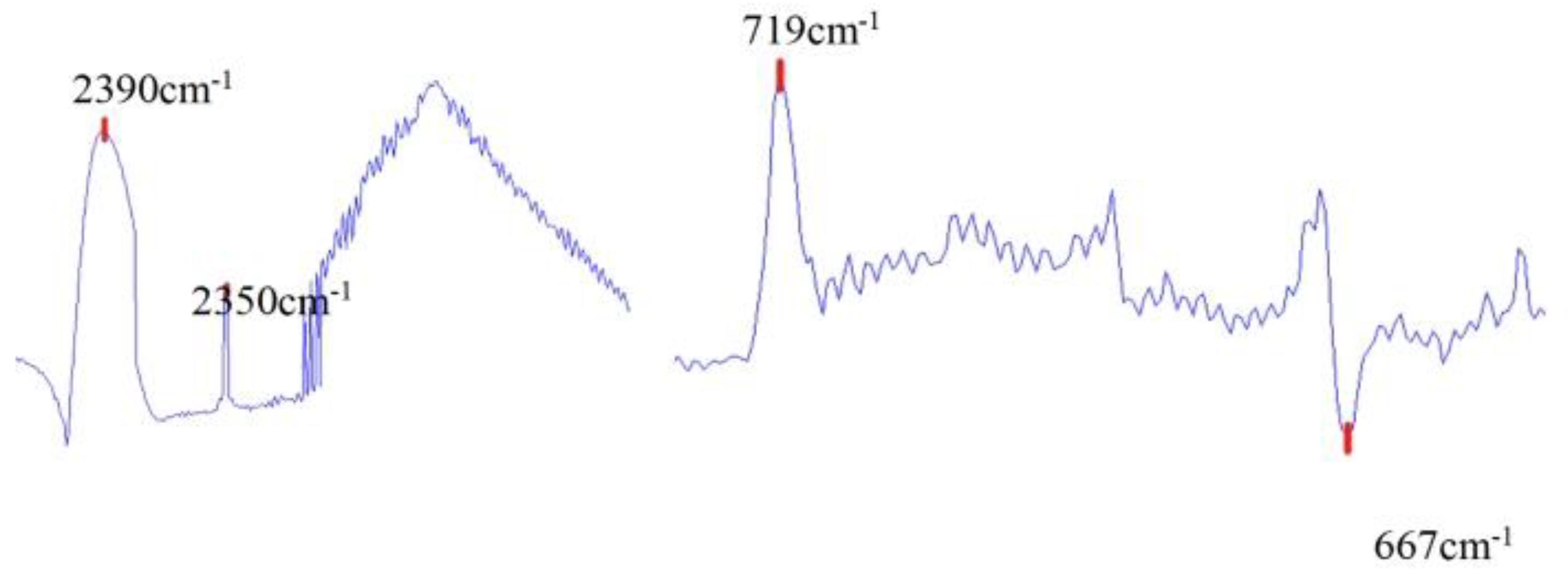
Based on the main emissions of the aeroengines and the measured infrared spectral data of the aeroengines, the peaks of the three most likely products of combustion, CO2, H2O and CO, were compared and analyzed. It was found that in the spectral curve, the characteristic peaks of CO2 at 667cm-1 and 2349cm-1 were obvious and stable, the spectrum of CO at the characteristic band of 2000-2222cm-1 gradually weakened with the increase of rotational speed, and the characteristic peaks of H2O were not obvious and not informative. Therefore, the two characteristic peaks (667cm-1 and 2350cm-1) of CO2 in the mid-wave infrared (MWIR) region (400-4000cm-1) and the two stable and obvious characteristic peaks (719cm-1 and 2390cm-1) in the measured spectral curve were selected for the construction of spectral feature vectors. In this paper, the spectral feature vectors are constructed based on the BTS, and the numerical difference of the BTS is related to the exhaust temperature of the aeroengines as well as the concentration and temperature of the gas in the hot jet.
Four characteristic peaks in the MWIR region of the BTS of the measured aeroengine hot jet were selected for the construction of spectral feature vectors, and the corresponding wave numbers of the peaks are 2350cm
-1, 2390cm
-1, 719cm
-1, 667cm
-1, their locations are shown in
Figure 2 below:
Spectral feature vectors
are composed of individual spectra by calculating the peak difference between the 2390 cm
-1 and 2350 cm
-1 and the peak difference between the 719 cm
-1 and 667 cm
-1.

Affected by the environment, the peak positions of the selected characteristic peaks may be shifted, the four characteristic peaks of 2350cm
-1, 2390cm
-1, 719cm
-1 and 667cm
-1 of the experimentally measured infrared spectral data are extracted from the area range where the maximum and minimum peaks are located for the extraction of spectral feature vectors, and the specific selection of the threshold range is shown in
Table 1:
3. Spectral Eigenvector Classification Methods
This section provides a brief description of the mainstream classifiers SVM [
13,
14,
15], XGBoost [
16,
17], CatBoost [20,21,22], AdaBoost [
18], Random Forest [23], LightGBM [
19], Neural Network [24,25] classifiers.
The current mainstream classification methods are supervised learning methods, unsupervised learning methods, semi-supervised learning methods, reinforcement learning methods, deep learning methods and ensemble learning methods. Supervised learning methods are methods that use training data with labels to construct a model that is used to classify new samples, including decision tree, support vector machines (SVM), and logistic regression. Ensemble learning methods include Bagging and Boosting, where Bagging is characterized by the absence of strong dependencies between individual evaluators, a series of individual learners can be generated in parallel, representing the algorithm Random Forest; Boosting is characterized by the presence of strong dependencies between individual learners, a series of individual learners are basically Boosting is characterized by a strong dependency relationship between individual learners, and a series of individual learners basically need to be generated serially, representing algorithms such as AdaBoost, XGBoost, LightGBM, etc.
In view of the characteristics of the aeroengine infrared spectral data and the way of measurement in this paper, it is more appropriate to use the training data set, test data set and label set for model training to carry out classification and prediction. In this paper, SVM, XGBoost, CatBoost, AdaBoost, Random Forest, LightGBM, and Neural Network algorithms are used in conjunction with spectral feature vectors to complete the classification task of the aeroengines.
① Support Vector Machine (SVM) classification method
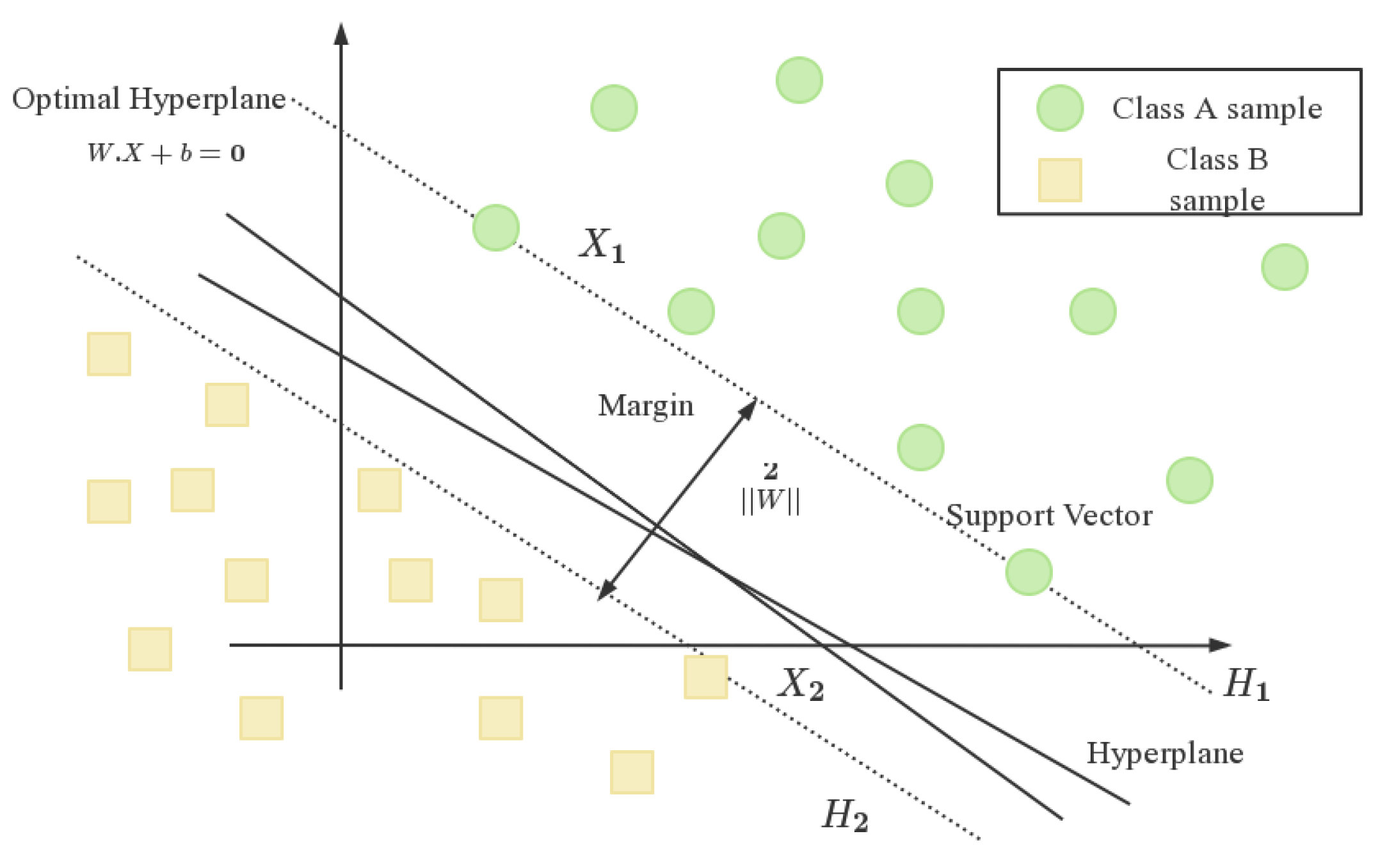
SVM is a kernel function based classification algorithm machine learning binary classification model for both binary and multi classification problems.The main task of SVM model is to find the optimal over-planning for classifying the data points. For binary classification , SVM algorithm is shown in
Figure 3:
SVM classifies the data by hyperplane
, which can be expressed as

Calculate the hyperplane equations, the thresholds on both sides, and the optimization function for the best vector in the hyperplane. Define the margin line as passing through the nearest point in each class to obtain the equation for the boundary line as:

where,

is the hyperplane equation,

is the edge line equation for the positive region, and

is the edge line equation for the region with negative values.
Finding the distance between two edges can be accomplished by the following:

Maximize the margin line function to find the optimal threshold. The final SVM model is obtained:

SVM algorithm is suitable for high-dimensional spatial data processing, and has good performance in the field of text classification and image recognition, and at the same time, it can maintain good performance when small sample data is processed. SVM algorithm is also one of the most commonly used algorithms in current classification tasks.
②XGBoost classification method
XGBoost is an efficient classification and regression algorithm based on gradient boosted decision trees.XGBoost algorithm generates multiple decision trees in an iterative manner by integrating weak classifiers and training based on the residuals of the previous decision tree, and finally integrates multiple decision trees to improve the performance of the model and complete the classification.
In the XGBoost classifier, firstly, the training data set , the differentiable loss function , multiple weak learning M and the learning rate , are defined as the input parameters of the XGBoost model.
Initialization operations are performed on the model using constant values:

As the model starts from 1 iteration to M, the gradient is first calculated:

Second, calculate the Hessians matrix:

Fit the base learner to the training data set

evolutionary optimization of the formula is obtained:

Finally, the model is updated:

After the iteration is completed, the output of the final model equation is:

The XGBoost algorithm shows higher performance and efficiency in classification tasks on large-scale data sets.The XGBoost algorithm has the following advantages: firstly, it is highly efficient in handling large-scale data; it supports L1 and L2 regularization, which helps to prevent over-fitting; it is able to automatically select the important features, which reduces the work of feature engineering; it supports a variety of loss functions, which can handle multiple tasks, such as regression, classification, sorting, etc.; it is able to utilize multiple core processors in parallel. , sorting, and many other tasks; it is able to parallel computation using multi-core processors.
③AdaBoost classification method
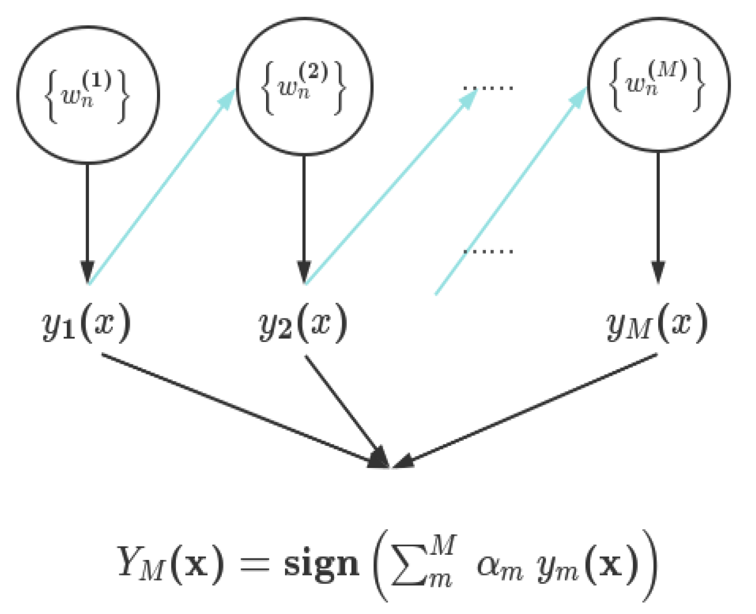
AdaBoost algorithm is an adaptive enhancement algorithm for ensemble learning, the method is used to add and train new weak decision makers serially and weight the combination of decision makers so that the loss function continues to decrease until the addition of decision makers is ineffective, and finally all the decision makers are integrated into one whole for decision making.The AdaBoost algorithm is illustrated in
Figure 4:
First, the AdaBoost algorithm defines the training data set as, where ,the learner is defined as, the training session is set as, and the initial weight distribution is set as, where.
During the training iterations, the base learner
is first obtained by learning using a training data set with a distribution of power values:

Based on
, calculate the error rate of the learner
on the training data set:

Calculate the coefficient
of
:

Update the sample weight distribution

:

where,
is the normalization factor,

, which ensures that all

constitute a distribution.
The final output of the model
:

AdaBoost algorithm can adapt to the respective training error rates of weak learners, and is suitable for a variety of classification problems that do not require a lot of tuning.AdaBoost algorithm has the following advantages, it is easy to implement and adjust, and does not require too much parameter tuning; it is not easy to over-fit, and by iteratively lowering the weight of the wrong samples, the risk of over-fitting can be reduced; it can be used in conjunction with a variety of basic classifiers of weak learners such as decision trees, neural networks, etc.; it is applicable with unbalanced data sets and deals with unbalanced data through the adjustment of weights.
④ Light Gradient Boosting Machine(lightGBM) classification method
Developed by Microsoft team, LightGBM is a fast classification and regression algorithm based on gradient boosting decision tree, which is an optimized improvement of XGBoost algorithm.The improvement of LightGBM algorithm lies in the use of Histogram algorithm to process the data, Leaf-wise growth strategy to construct the tree, and the optimal splitting point by optimizing the objective function to select the optimal splitting point. It can be understood that LightGBM algorithm is a combination of XGBoost, Histogram, GOSS, and EFB algorithms.
The construction of LightGBM algorithm model is shown in
Figure 5:
LightGBM algorithm has fast, efficient, distributed structure and high performance characteristics can be used in sorting, classification, regression and many other machine learning tasks.LightGBM algorithm's advantages are: the introduction of the histogram algorithm reduces the time complexity consumed by traversal; during the training process, the one-sided gradient algorithm can filter the samples with small gradient to reduce the amount of computation; the Leaf- wise growth strategy to build the tree is also introduced to save the computational cost; the optimized feature-parallel and data-parallel methods are used to accelerate the computation, and the ticket-parallel strategy can be adopted when the data volume is large, and the cache is also optimized.
⑤ CatBoost classification method
CatBoost algorithm is an open source gradient boosting classification algorithm that uses symmetric binary tree structure for training and introduces a new loss function and optimization method.The base learner of CatBoost algorithm adopts a fully symmetric binary tree, which is based on symmetric decision trees (oblivious trees).This algorithm has fewer parameters, supports categorical variables, and a highly accurate GBDT framework, which can efficiently and reasonably process categorical features. It also proposes methods for dealing with gradient bias and prediction shift problems to improve the accuracy and generalization ability of the algorithm.
First, the CatBoost algorithm defines the training data set as

, and then the prediction set is as:

where, represent the regression trees and K is the number of regression trees. The formula shows that given an input, the output K regression tree adds up to the predicted values.
Define the objective function, the loss function, and the regular term to obtain the optimized objective function:

where,

.
CatBoost algorithm automatically handles category features and excels in both performance and effectiveness.The advantages of CatBoost algorithm are strong ability to handle category features, robustness, high performance, support for GPU acceleration, automatic feature selection and friendly to sparse data.
⑥Random Forest (RF) classification method
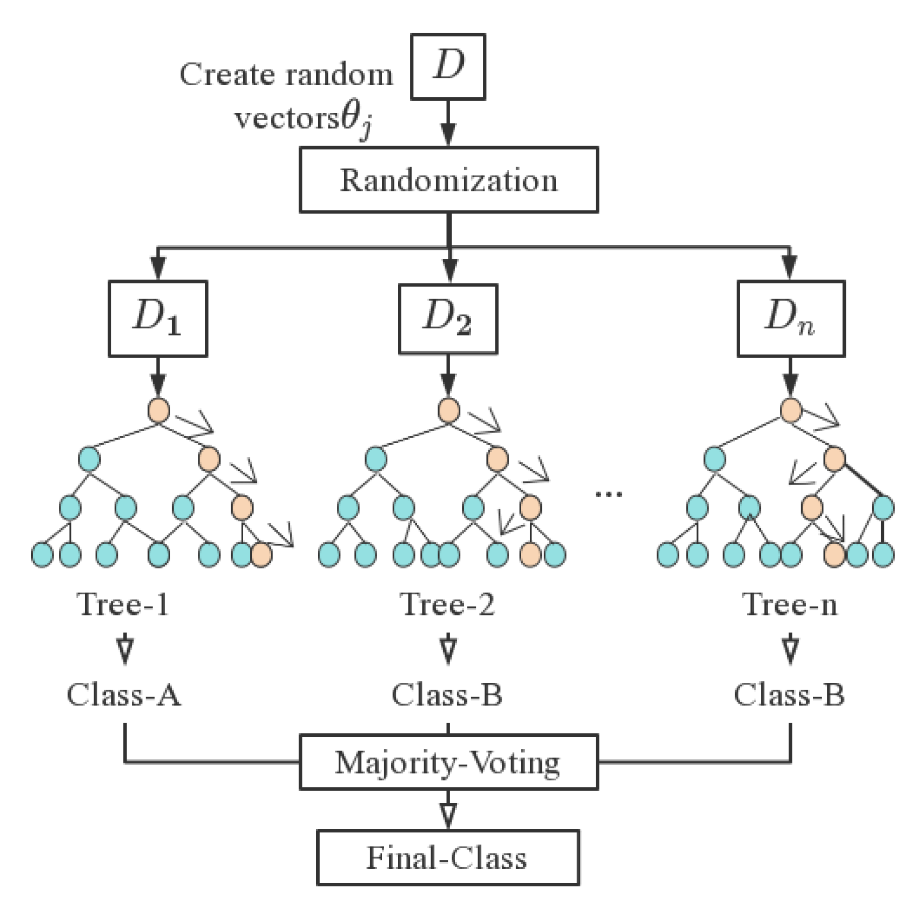
RF is a supervised classification algorithm based on decision trees, which predicts classification results by assembling multiple decision trees.In 2001 Bremen combined classification trees into a random forest, i.e., randomized the use of variables (columns) and the use of data (rows) to generate many classification trees, and then aggregated the results of the classification trees. RF improves the prediction accuracy without significant increase in arithmetic.
RF is an extension of Bagging, the model input is defined as the training data set

, the base learning algorithm

and the number of training rounds T.
Conduct the T iteration of the learning algorithm, and the base learning algorithm

is updated in the iteration:

The output model
was obtained

RF is an extended variant of Bagging that further introduces the selection of random attributes in the training process of decision trees based on the decision tree as the base learner to build the Bagging integration. RF is shown in
Figure 6:
RF increases the differences between classification models by constructing different training data sets, thus improving the extrapolated prediction ability of the combined classification model. Through training, a sequence of classification models is obtained, and then they are used to form a multi-classification model system with the final classification decision as, as in Equation 22.
RF supports parallel processing and does not require normalization of features or processing of missing values; the model is stable, generalizes well and can output the importance of features; it uses Out of Bag and does not need to divide the test set separately. However, it takes a long time to construct the tree and the algorithm occupies a large amount of memory
⑦ Neural Network (NN) classification method
Neural Networks use neural networks for classification by modeling the way the human nervous system works.
A neuron can be understood as a multi-dimensional linear function, or a unit that does a linear combination. In the figure
is the input to the neuron,

is the threshold function, and f is the output.

is the weights in the linear combination, or the slope of the line. To facilitate the representation and computation of a large number of weights, they are generally represented as vectors or matrices.
NN is the current mainstream algorithm used for image classification, which supports automatic learning of features and patterns in the data, and has good adaptability to non-linear relationships; its computational units support highly paralleled computation, which speeds up the training speed; its distributed storage and processing improves the fault-tolerance of the system; and it has a good generalization ability after sufficient training, and is able to perform accurate classification on unseen data for accurate classification. When dealing with large-scale data and complex tasks, NN requires longer training time and larger computational resources, and can be improved in terms of reasonable choice of network structure, adjustment of hyper parameters and avoidance of over-fitting to address the problem.
4. Experiments and the Results
This section describes the specific experimental process and methodology of the aeroengine classification experiment, which consists of three parts: aeroengines, spectral acquisition experimental design, data set production and spectral feature vector extraction, and classification prediction result accuracy assessment. Among them, the part of aeroengines spectral measurement experiment design describes the field arrangement of aeroengine hot jet spectral measurement experiment, the part of data set fabrication and spectral feature vector extraction describes the training data set, test data set, label set production, and spectral feature vector extraction adopted in the classification experiment, and the classification prediction result accuracy assessment section evaluates the prediction of the classification method used in this paper on the real data set.Finally, the experimental result graphs and evaluation index tables are provided.
4.1. Experimental Design of Aeroengine Spectral Measurement
First, the infrared spectral data of three different aeroengines’ types was collected by field measurement. The Fourier Transform Infrared Spectrometers used in the experiment are the EM27 and the telemetry FTIR developed by the Aerospace Information Research Institute. The specific parameters of the two devices are shown in
Table 2:
The experimental preparation stage requires the experimental devices to be set up according to the experimental conditions in the external field.
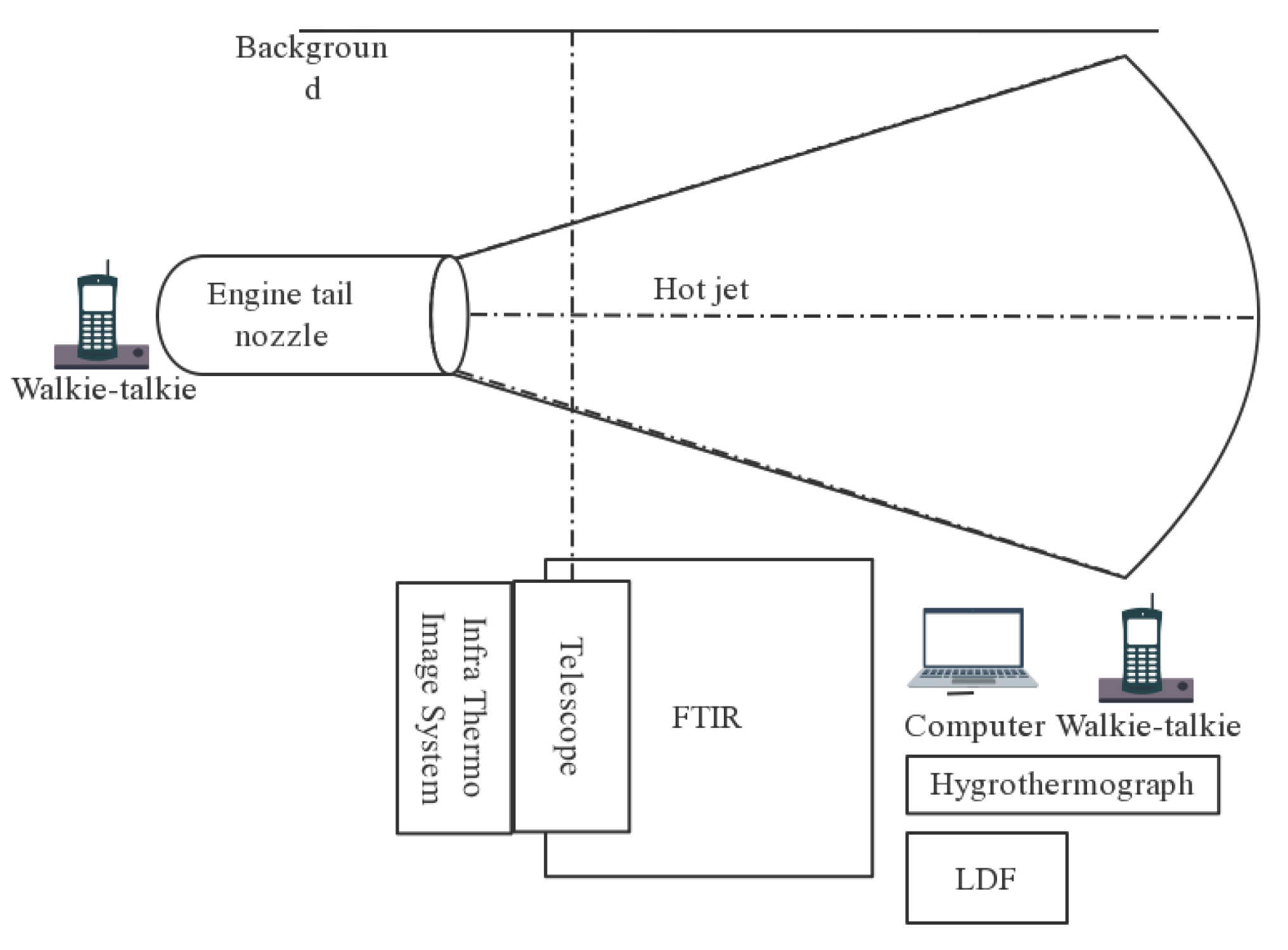
Firstly, according to the spectrometers' field of view angle and hot jet information, the measurement distance was adjusted with a telescope to make the hot jet fill the field of view. The EM27 and telemetry FTIR were mounted on two tripods respectively, and the laser and scope were used to assist the aiming, and the height and angle of the tripod were adjusted so that the optical axis of the equipment was aligned with the centre of the aeroengine tail nozzle.
Next, after fixing the position, increase the tripod counterweight to improve stability, and fix the thermos-hygrometer near the measurement position. Determine the position of the infrared thermal camera to clearly photograph the hot jet to be measured.
Finally, the workstation display time and the control room control system time were strictly aligned. After the cooling is completed, run the two upper computer software respectively, set the measurement mode, spectral resolution and superimposed number of times in EM27 software, and use the displayed ADJUST value to fine-tune the tripod angle until the maximum value is taken. After the settings were completed, the spectral data when the aeroengine was not started were collected as background data.
The layout of the experimental site is shown in
Figure 8:
During the experiment, real-time communication was conducted with the person in charge of the aeroengine through walkie-talkie, requesting real-time prompts when the rotational speed was changed, and requesting that each test rotational speed be stabilized for 1 min as much as possible (since 100% rotational speed is difficult to be maintained for 1 min in the actual measurement process, the amount of spectral data collected in this part is small). The ambient temperature and humidity were recorded at each adjustment of the rotational speed. The environmental factors of the experiment were recorded as shown in
Table 3:
4.2. Data Set Production and Spectral Feature Vectors Extraction
Based on the actual measurements of the aeroengines in the field, the controllable rotational speed ratios differed for each engine. Therefore, the infrared spectral data of 70%, 80%, 90% and 100% of the maximum rotational speed ratios common to the three aeroengines were selected as the data source. There are a total of 211 spectral data in the data source, and after removing 2 erroneous data, 209 reliable data remain.
The experiments were conducted according to the aeroengines for the measurement of infrared spectra, so the data were divided according to aeroengines. To verify the feasibility of the spectral feature vector classification algorithm in this paper, random sampling of the data source is required to generate the training and test datasets with labels. In the ratio of 3:1, the data sources were randomly sampled to divide the training and test datasets, and the datasets were generated with a total of 158 spectral data with 1 labeled set data for Train Dateset and 51 spectral data with 1 labeled set data for Test Dateset.
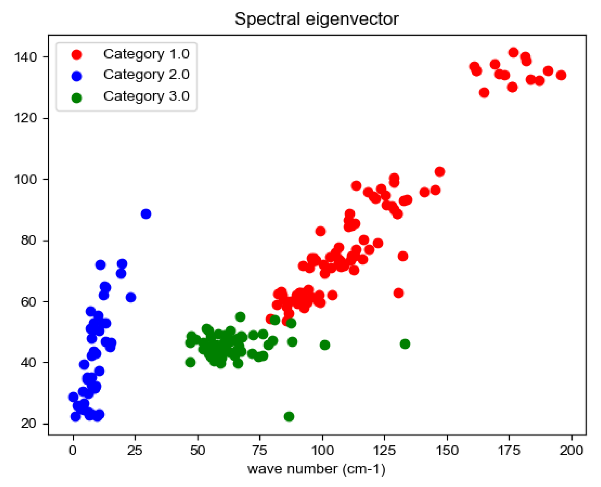
The spectral features of the experimentally measured the three aeroengines at 70%, 80%, 90% and 100% of the maximum rotational speed were counted, and the statistical results were plotted as a two-dimensional feature map (as shown in the figure below), where the horizontal coordinates are
, and the vertical coordinates are
,as shown in
Figure 9.
The aeroengines of the three aircraft are relatively sufficient for fuel combustion, and the exhaust gas spectrum at different speeds is close, so the gas composition characteristics of the gas discharged at the cruise speed of the three aircraft aeroengines are compared. Due to the different environment, temperature and other conditions of the three field experiments, the spectrograms were compared after deducting the background. From the two-dimensional feature map, it can be seen that the two-dimensional feature vectors of the three types of engines have been distributed in different regions of the feature space, and the overlap region between each other is relatively small, so the constructed spectral feature vectors initially have the ability to classify.
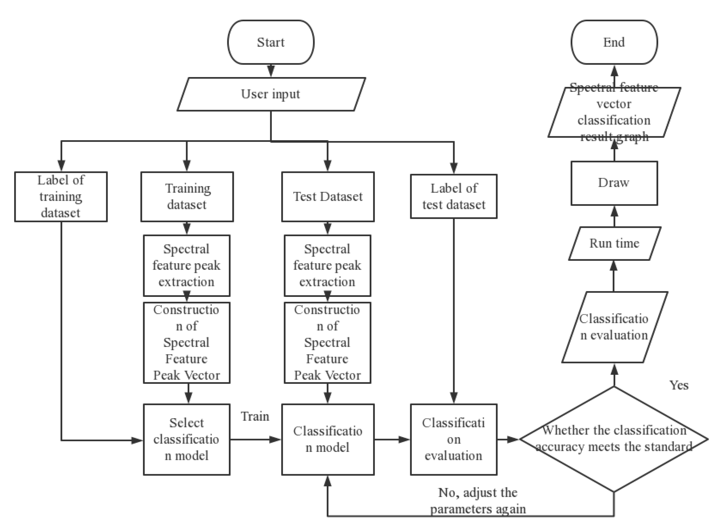
The spectral feature vectors and the classifier are combined to train and predict the spectral data. The flow chart of the classification algorithm used in the experiment is shown in
Figure 10:
4.3. Assessment of the Accuracy of Classification Prediction Results
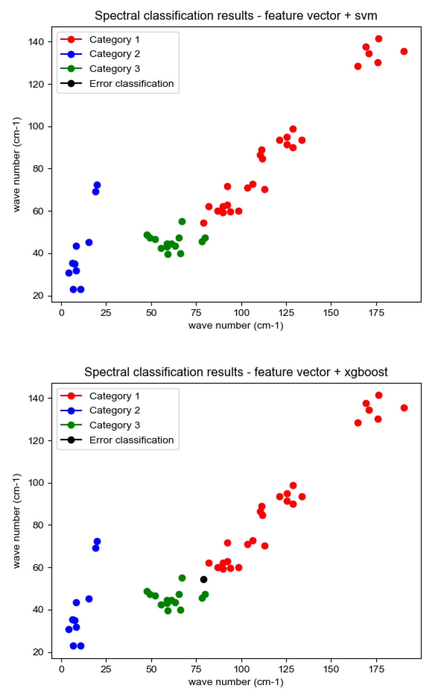
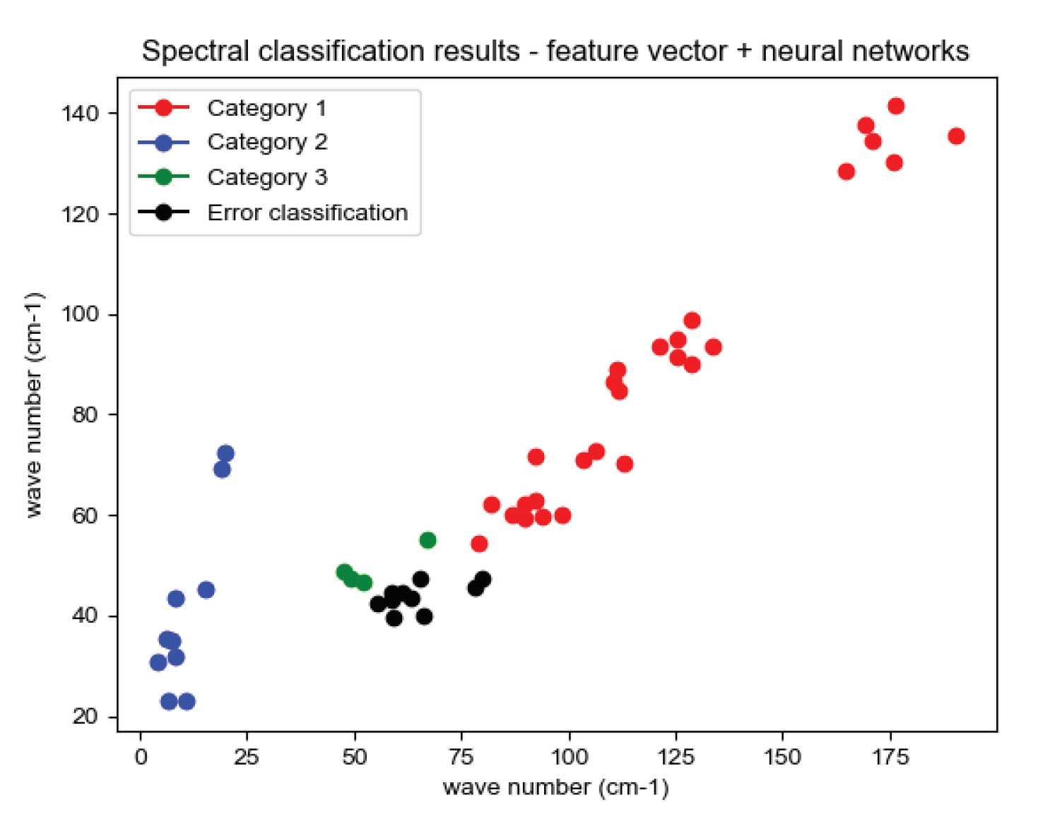
The experimentally constructed infrared spectra training data set and test data set are tested for classification of spectral feature vectors with seven classifiers, SVM, XGBoost, CatBoost, AdaBoost, Random Forest, LightGBM, and Neural Networks, and the classification results are shown in
Figure 11:
Where, red, green and blue represent the feature vectors of the three correctly classified aeroengine hot jet infrared spectra, while black represents the misclassified feature vectors. The evaluation criteria for aeroengine spectral classification consist of accuracy, precision, recall, F1 value (F1-score) with confusion matrix [23]. It is assumed that the instance is a positive class and is predicted to be positive, i.e., true class, denoted as TP (True Positive), and if it is predicted to be negative, i.e., false negative, denoted as FN (False Negative), and on the contrary, if the instance is a negative class, it is predicted to be positive, i.e., false positive, FP (False Positive), and if it is predicted to be negative, i.e., true negative. TN (True Negative). Based on the above assumptions, the accuracy, precision, recall, F1 value and confusion matrix of the evaluation criteria are defined separately:
① Accuracy: Proportion of correctly categorized samples to total samples.
② Precision: The ratio of the number of samples correctly predicted to be positive to the number of all samples predicted to be positive.
③ Recall :The ratio of the number of samples correctly predicted to be in the positive category to the number of samples in the true positive category.
④ F1-score: The F1 value combines the harmonic mean of precision and recall and is used to measure the overall performance of the model.
Among them, Represents Precision, R represents Recall.
⑤ Confusion matrix : The confusion matrix shows how well the classifier categorized the different categories, including true examples, false positive examples, true negative examples, and false negative examples. It shows the difference between the actual and predicted values, and the values on the diagonal of the confusion matrix indicate the number of correct predictions made by the classifier for that category.
According to the above five evaluation criteria for the algorithm of combining spectral feature vectors and classifiers used in this paper to predict the labels of the prediction set, the prediction results are shown in
Table 5:
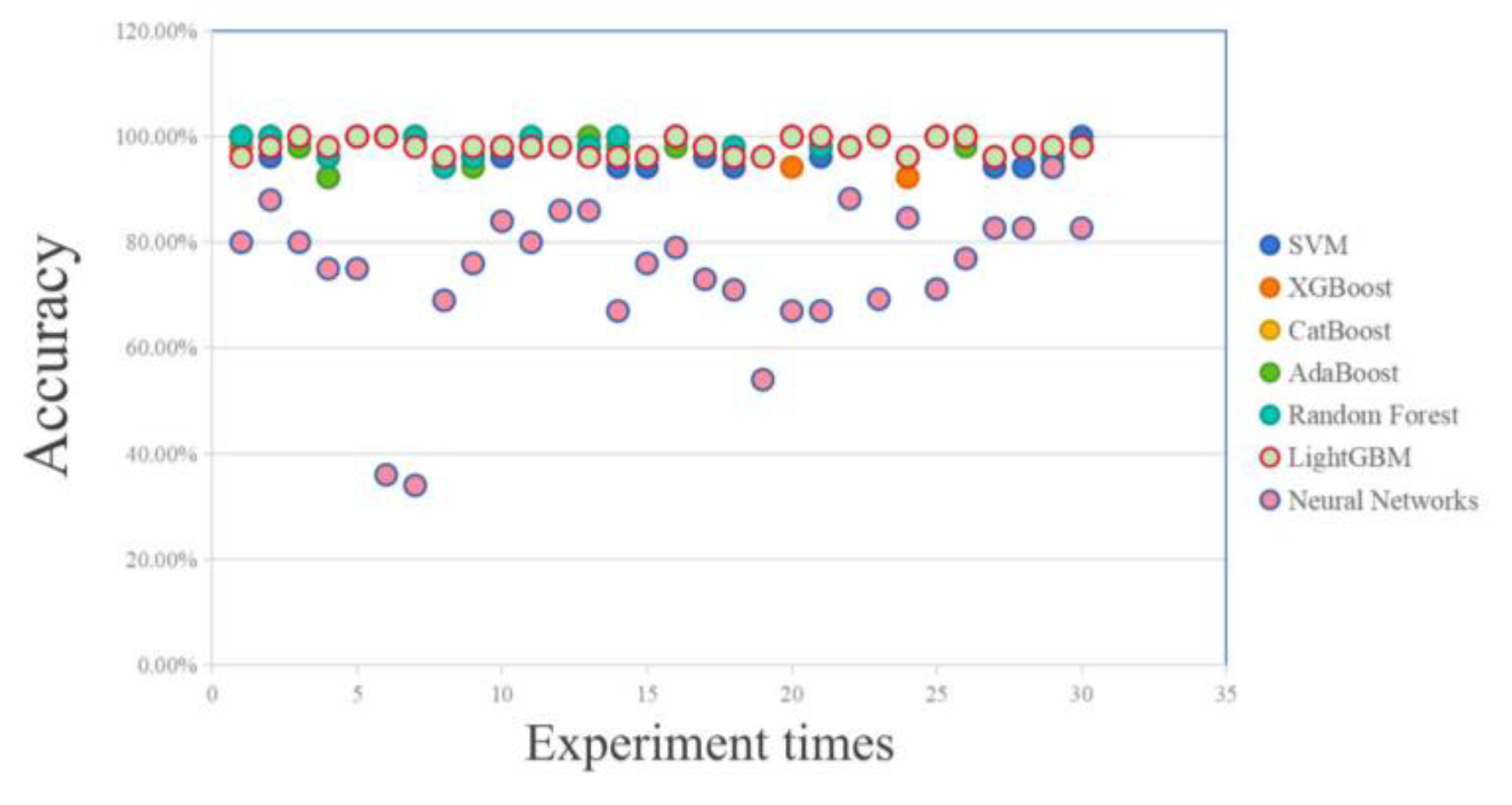
The evaluation criteria for combining the aeroengine hot jet infrared spectral feature vectors with the seven classifier combination algorithms are analyzed according to the above table. Since the experimental data set is generated by random numbering based on the experimental measurement spectra, the probability of predicting the data has a certain degree of chance. Therefore, several experiments were conducted to evaluate the overall accuracy, and the correctness is shown in
Figure 12:
The data from the 30 experiments conducted were counted to obtain the classifier prediction probability statistics as shown in
Table 7:
According to
Table 7, in terms of accuracy, CatBoost, AdaBoost, Random Forest and LightGBM maintain good accuracy in accuracy, and can achieve relatively accurate prediction in multiple experiments. The prediction accuracy of SVM is average, while Neural Networks is less effective in the classification of spectral feature vectors. In terms of time measures, the seven methods have a similar running time, while the CatBoost is slightly slower. Overall, the mainstream classifiers have achieved a relatively ideal classification accuracy.


 is the hyperplane equation,
  is the edge line equation for the positive region, and
  is the edge line equation for the region with negative values.


 evolutionary optimization of the formula is obtained:


 :
:
 , which ensures that all
  constitute a distribution.
 , and then the prediction set is as:

 .
. , the base learning algorithm
  and the number of training rounds T.
 is updated in the iteration:

 is the threshold function, and f is the output.
  is the weights in the linear combination, or the slope of the line. To facilitate the representation and computation of a large number of weights, they are generally represented as vectors or matrices.