
Submitted:
22 December 2023
Posted:
25 December 2023
You are already at the latest version
Abstract
Space and water heating for residential and commercial buildings amount to a third of the European Union’s total final energy consumption. Approximately 75% of the primary energy is still produced by burning fossil fuels, leading to high greenhouse gas emissions in the heating sector. Therefore, policymakers increasingly strive to trigger investments in sustainable and low-emission heating systems. This study forms part of the “Roll-out of Deep Geothermal Energy in North-West-Europe”-project and aims at quantifying the spatial heat demand distribution in the Interreg North-West-Europe region. An open-source geographic information system and selected Python packages for advanced geospatial processing, analysis, and visualization are utilized to constrain the maps. These were combined, streamlined, and optimized within the open-source Python package PyHeatDemand. Based on national and regional heat demand input data, three maps are developed to better constrain heat demand at a high spatial resolution of 100*100m2 for the residential and commercial sectors, and for both together (in total). The developed methodology cannot only be applied to transnational heat demand mapping but also on various scales ranging from city district level to states and countries. In addition, the workflow is highly flexible working with raster data, vector data, and tabular data. Results reveal a total heat demand of the Interreg North-West-Europe region of about 1,700TWh. The spatial distribution of the heat demand follows specific patterns, where heat demand peaks are usually in metropolitan regions like for the city of Paris (1,400MWh/ha), the city of Brussels (1,300MWh/ha), the London metropolitan area (520 MWh/ha), and the Rhine-Ruhr region (500 MWh/ha). The developed maps are compared with two international projects, Hotmaps and Heat Roadmap Europe’s Pan European Thermal Atlas. The average total heat demand difference from values obtained in this study to Hotmaps and Heat Roadmap Europe is 24 MWh/ha and 84 MWh/ha, respectively. It is assumed that the implementation of real consumption data is an improvement in spatial predictability. The heat demand maps are therefore predestined to provide a conceptual first overview for decision-makers and market investors. The developed methods will further allow for anticipated mandatory municipal heat demand analyses.

Keywords:
heat demand map
; geographic information system
; python
; spatial data analysis
; renewable energy
; sustainable energy
1. Introduction
Reducing greenhouse gas emissions by replacing fossil fuel-based energy systems with sustainable and climate-neutral systems is a major focus of the Green Deal of the European Union (EU) [1]. As 75% of the primary energy and approximately 50% of the thermal energy are still produced from fossil fuels, the EU has funded several projects regarding an efficient heat demand (HD) mapping to address possibilities for the implementation of sustainable heating systems such as the dimensioning of heat pumps, the setup, and extent of district heating networks or the required power of a (geothermal) power plant [2,3,4,5]. The European Commission further proposed in the recast Energy Efficiency Directive that heating plans will be mandatory for municipalities above a threshold of 50,000 inhabitants, which will require comprehensive heat demand analyses on local to regional scales. As shown by some countries that already performed a heat planning process, such as Denmark, the Netherlands, Scotland, and parts of Germany, it is to be expected that not all municipalities will have the corresponding consumption data available in a standardized form and of the same resolution, so that in particular heat demand analyses at the district to regional level will require tools for harmonizing and evaluating heterogeneous consumption data sets.
To address a scenario in which local to regional heat demand analyses with appropriate and user-friendly tools will become mandatory, this study has been conducted within the framework of the Interreg North-West-Europe area (Interreg NWE) project “Roll-out of Deep Geothermal Energy in North-West-Europe” (DGE-ROLLOUT) [6,7,8,9]. As part of the project, the goal of this study was to produce harmonized heat demand maps for the project area on one hand, and thereby develop a sufficient method that can be used for tool-development for heat demand analysis on variable input data sets and scales on the other hand. According to the Energy Efficiency Directive, the member states of the EU must map their HD on a high spatial resolution [10]. National HD data of several member and non-member states were available for this study (Belgium [11], Switzerland [12], Germany [13,14,15,16,17], France [18,19], The Netherlands [20,21], and Scotland [22]).
The HD describes the energy () needed for space and water heating over a certain area (e.g. ) and time period (e.g. one year after the Julian calendar with 365/366 days). Usually, the heating differs between the residential/domestic and commercial sectors. Residential buildings are exclusively used for private usage, e.g. single- or multi-family buildings. Commercial buildings refer to any property used for business activity, e.g. office, retail, and lodging. The commercial sector on the DGE-ROLLOUT HD map also includes some institutional buildings, e.g. medical, educational, religious, and governmental buildings. Industrial, military, and infrastructural buildings are not included in the HD maps as their data are not publicly available and require individual approaches to characterize the heat sources and sinks, e.g. via a pinch analysis.
For the development of an HD map, a top-down or a bottom-up approach can be used, which differ fundamentally in their methodology (Figure 1). The first calculates HD on a large scale, usually on a national level or on lower Nomenclature of Territorial Units for Statistics (NUTS), while using publicly available, low-resolution data. The latter uses high-resolution data on a regional level, usually a city or a Local Administrative Unit (LAU). However, this more detailed approach significantly increases the computational and processing requirements. Because this might represent a hurdle for many municipalities in local to regional heat demand analysis as a fundamental element of municipal heat planning, methodological simplifications as preparation for the implementation of end-user tools are inevitable.
The two projects with the largest and most comprehensive dataset for spatial mapping of HD on a European level are Hotmaps [24] and the Pan European Thermal Atlas of Heat Roadmap Europe (HRE) [25]. Both projects use well-designed top-down approaches, based on a strong level of scientific expertise [26,27,28,29,30]. The Hotmaps project uses a statistical approach, whereas HRE uses an econometric approach. Both projects present their resulting heat demands on hectare resolution (). Besides these two projects, the development of HD maps has become an emerging subject of research in recent years. A profound literature review of HD maps until 2019 has been compiled by [31]. A detailed analysis is usually done at the city or district level, aiming at evaluating the (pre-) feasibility of district heating systems or regional development plans [32,33,34,35]. The traditional approach to developing HD maps is to use a geographic information system such as QGIS or ArcGIS [23,36,37]. Recently, more approaches using scripting languages, like R or Python, appear [38,39,40]. Since the data sets and methodologies are usually not publicly accessible, these local studies were not included in this study. An exception is a recent study for the Walloon region in Belgium, where no other HD data are available [41]. Many of the aforementioned studies do not provide the tools (i.e. scripts) to replicate the results. Further, they usually focus on smaller regions whereas the developed methodology in this study is not restricted to any administrative level or level of resolution.
Within the framework of this study, the open-source Python package PyHeatDemand was developed [42]. It does not aim at replacing any of the already developed heat demand mapping methods but rather aims at providing a methodology for administrative entities to harmonize heat demand data for better district heating plans. Three HD maps of the Interreg NWE area are presented in this study applying the developed procedures using publicly available consumption data to identify hotspots of the residential HD and the commercial HD, and both combined on a hectare scale for the observation period of one year (Julian calendar). The developed approach is easy to apply to different categories of data, allows for the reproducibility of the outcomes, a constant update of the maps once new data becomes available, and an extension of the study area for previously unmapped territory. The resulting HD maps are validated against the HD maps from Hotmaps and HRE (only a top-down approach). A combination of a bottom-up and top-down approach is implemented to deliver a higher resolved result than previous mapping projects. Major sweet spots for investment projects, for example, heat production from deep geothermal power plants using doublet systems or the extension of existing or development of new district heating systems, are assumed in areas with a high degree of urbanization, as these areas have usually existing district heating networks and a high customer density.
2. Materials and Methods
2.1. General Heat Demand Map Workflow
The creation of the heat demand maps follows a general workflow (Figure 2) followed by a data-category-specific workflow for the five defined heat demand input data categories (Table 1). Depending on the scale of the heat demand map (local, regional, national, or even transnational), a global polygon mask is created from the provided administrative boundaries of for the entire administrative unit (Interreg NWE region) with a cell size of 10 km by 10 km, for instance, and the target coordinate reference system (). This mask is used to divide the study area into smaller chunks for a more reliable processing as only data within each mask will be processed separately. If necessary, the global mask will be cropped to the extent of the available heat demand input data and populated with polygons having already the final cell size such as 100 m x 100 m. It is also possible to refine a previously coarser polygon mask using a self-implemented QuadTree [42] algorithm until the final resolution of i.e. 100 m is reached. In that case, only the areas with a high data density will display cell sizes of the final resolution while areas of low data densities will be combined. This also allows for identifying areas with only a few data points but large heat demands and vice versa. For each cell, the cumulated heat demand will be calculated. This was first done without utilizing spatial indexing. At a later stage, spatial indices [RTree [43] were implemented with a significant decrease in computing times. The final regular polygon grid will be rasterized and merged with adjacent global cells to form a mosaic, the final local to transnational heat demand map. If several input datasets are available for a region, i.e. different sources of energy, they can either be included in the calculation of the heat demand or the resulting rasters can be added to a final heat demand map.
The QGIS long-term release [v. 3.28.11, 44] is used to perform simple spatial operations to verify the processability and quality of the generated data. Python [v. 3.10., 45] including different open-source libraries such as GeoPandas [v. >= 0.14.0] and Shapely [v. > 2.0.2, 46,47] are used for processing the data, in particular for advanced geospatial operations and analysis. The Rasterio package [v. >= 1.3.9, 48] is further used to create the raster data. The developed workflow can be executed in Jupyter Python Notebooks [49] allowing for reproducible outcomes or recomputation of the results once new input data is available. All methods required to create the heat demand maps are also available in the open-source Python package PyHeatDemand [42] referenced in the Data Availability Statement which was created within the framework of the DGE-ROLLOUT project. The pure Python implementation guarantees the reproducibility of the results and eliminates manual data manipulation in geoinformation systems which are now only used for verification, quality control, and map creation.
2.2. Data Categories 1 and 2
The processing of data categories 1 and 2 follows similar workflows and corresponds to a bottom-up approach. The heat demand input data of category 1 are already displayed as a raster or a polygon grid, usually with a spatial resolution of . The raster will be vectorized to continue working with a polygon grid containing the heat demand data. The heat demand input data of category 2 are buildings of similar age classes and energy requirements, grouped as one statistical unit containing the heat demand data (Figure 3.1 & Figure 4 top). Further, the heat demand data can also be represented as street segments (LineStrings). Both data categories (1 & 2) are intersected with a local mask layer consisting of polygons (Figure 3.2) or a different target resolution. This results in individual polygon fragments inside each mask-polygon j. The HD of the intersected statistical units is summed up for each mask polygon and calculated according to their share of area (Figure 3.3).
For regions that have not provided any input heat demand data, the Hotmaps HD data has been used in this study instead. Since Hotmaps data is given with a high spatial resolution of raster cells in a different CRS, the methodology is identical as for HD of category 1. If no heat demand input data is available at all, top-down or bottom-up workflows can be utilized to estimate the heat demand (see section below).
2.2.1. Data Category 3
HD data of category 3 is provided as a point or polygon layer, where each point or polygon represents the sum of the HD for regions at the Local Administration Units level (LAU) for this study or any other administrative unit. The processing of this data corresponds to a top-down approach. The centroids of the polygons are then used for further processing. The spatial distribution of HD from Hotmaps is used to increase the resolution to . These Hotmaps data are summed up for each LAU and then compared with the provided heat demand input data. Equation (2) defines a scale factor for each LAU as the heat demand input data is divided by the summed-up Hotmaps HD data . Each Hotmaps HD grid cell is then multiplied with this scale factor. This process increases the spatial resolution of the provided heat demand input data using the solid scientific approach from Hotmaps (Figure 4). Alternatively, population density grids can be utilized to increase the spatial resolution of the data.
2.2.2. Data Category 4
Category 4 comprises all the unique processing methods for HD data, which could not be categorized within the previous formats. The calculation of HD for instance for the Netherlands as presented later is based on the absolute gas demand per postal code area. Gas is used for 84% of heat generation in the residential sector and as a total energy carrier [20,21]. Equation (3) has been defined to transform the gas demand into heat demand:
refers to the annual HD in the Netherlands in . is the gas demand in . is the net calorific value of natural gas, which is set to or, to use the correct unit directly, for this region [50]. The fraction of gas used for space heating and hot water heating is set to 72% [51] and 23% [52], respectively.
Using gas usage or the usage of any source of heat can be converted into a heat demand and corresponds to a very precise bottom-up approach using billing data. This becomes increasingly important with more and more decentralized and independent heat sources. The resulting heat demands for each energy source can later be aggregated to result in the final heat demand of a respective local cell.
For the Walloon region as another example, the HD is provided for each NUTS-3 region as image data [41]. This image data is georeferenced and the color code of each NUTS-3 is extracted as point data. The HD of each point corresponds to the predefined value ranges, here, the lower limit, defined by [41]. The point layer has been manually adjusted where the color code extraction was not successful. This point layer is used as the input for processing HD in category 3.
2.3. Development of the heat demand maps
The development of the workflow to create three standardized maps for the DGE-ROLLOUT project showing the annual heat demand on a hectare resolution (in as squares) is based on existing regional heat demand input data displaying a wide range of possible data formats. The regionally collected consumption data is publicly available through project partners, authorities, and research communities. In comparison to previous projects, real measurement data (billing data) is implemented to represent the spatial conditions as accurately as possible is implemented.
The provided HD data can be divided into two categories of quality and five categories of spatial presentation, based on the region (according to [53]) or the previous studies (Hotmaps, Heat Roadmap Europe), respectively (Table 1). The two categories of quality depend on whether the provided heat demand input data is calculated or originates from billing data (Figure 5). The latter can be interpreted as a bottom-up approach.
Since the heat demand input data is usually provided in a regional coordinate reference system (CRS), it has been transformed into the reference system used by the DGE-ROLLOUT project () to avoid distortions of the spatial data.
2.4. Statistical evaluations using Rasterstats library
The compiled heat demand maps were analyzed on a national scale using the zonal statistics of the Rasterstats Python library [54] in combination with simple algebraic calculations using the Pandas Python library [55]. Hereby, the zonal statistics only account for raster cells that actually hold a value. Cells, where no heat demand has been calculated, are not considered in these calculations.
Zonal statistics cannot only be applied on a national level but also on a regional level (e.g. states, communes) or a local level (cities, districts) to evaluate and summarize the respective heat demand for heat demand planning.
2.5. Development of heat demand difference maps
To further evaluate the quality of the merged DGE-ROLLOUT HD maps, Hotmaps and HRE have been used as references. The HD data from these projects are provided as raster cells for the entire region of this study but were using a top-down approach rather than using the combined bottom-up and top-down approach also integrating billing data like for this study. The transformation of these HD data is identical to HD data from category 1. Each raster cell from each DGE-ROLLOUT HD map has been subtracted from their Hotmaps and HRE counterparts to develop the difference maps (Figure 6). Equation (4) describes the HD difference for each raster cell.
The statistical dispersion of the average HD differences between the DGE-ROLLOUT and Hotmaps/HRE is presented in the form of violin plots, presenting a probability density of the HD differences. Six violin plots, two each for the residential, commercial, and total HD difference maps (HDDM) displaying the statistical dispersion. The plots present the mean values and the corresponding standard error of means as a distribution. Furthermore, the median of the mean values and the 25th and 75th quantiles are outlined.
3. Results
3.1. Heat demand maps
Using the developed workflow including the implementation of spatial indices, three maps developed in this study present the HD in units of energy over a certain area ( raster cells) and time period for the residential and commercial sectors and the summed-up HD of both sectors (Figure 7). Since the time period is always one year (Julian calendar), it is usually not displayed for the annotation of the units. HD values below 15 are not displayed in the maps, due to calculation inaccuracies and low significance for investment projects. Data tables summarizing the heat demand data are available in the appendix.
3.1.1. Areal Statistics
Areal statistics are presented prior to the results of the heat demand mapping. As the resulting maps extend over larger parts of Europe, the ellipsoidal area measurements accounting for the curvature of the earth when working on a larger scale are favored over the planimetric measurements usually used for local area calculations. The ellipsoidal areas were extracted from QGIS and implemented in the statistical analysis instead of using the planimetric values calculated by the designated GeoPandas and Shapely libraries [46,47] as they use the planimetric area measurement approach. Overall, the planimetric area data only measures about 93% of the ellipsoidal area. Hence, there would have been a significant error when using the planimetric measurements. The total area of the Interreg NWE region amounts to 842,824 . The northern part of France contributes 33.1% (279,030 ) followed by Great Britain with 19.6% (165,486 ) and the western part of Germany with 17.4% (146,607 ). The remaining countries contribute with less than 10% each to the total Interreg NWE region with as little as 0.3% (2,596 ) for Luxembourg (Table A1, Table A2, Table A3). Neglectable area differences occur between the regional areas and the national areas. The latter ones have a total planimetric area that is 4 larger and an ellipsoidal area that is 1 larger than the regional areas. This difference arose during the creation of the national layer.
3.1.2. National Results - Level 0 of the Nomenclature of territorial units for statistics
The total HD (residential and commercial combined) of the Interreg NWE region is approximately 1,727.2 (Table A1). The residential HD accounts for 65.38% (1,129.3 , Table A2) while the commercial HD accounts for 32.26% (557.1 , Table A3). The remaining 2.35% are attributed to the HD of Scotland (40.7 ) which was only provided as total HD and was not split in residential or commercial HD, respectively. The country with the highest total heat demand is Germany (only the NWE part) with 606.9 (35.1% of the total HD) split into 340.3 (30.1% of residential HD) and 266.5 (41.4% of commercial heat demand, Figure 8). Here, it is worthwhile mentioning that the state of Saarland also contributes to industrial heat demand to the total HD.
The two other major consumers are Great Britain with 24.5% of the total heat demand, 28.4% of the residential heat demand, and 18.3% of commercial heat demand, and France (only NWE part) with 21.0%, 23.6%, and 17.2%, respectively (Figure 8). These three countries account for ∼80% of all three calculated heat demands. The remaining countries have shares ranging from 0.4% (7.5 total) to 6.7% (75.3 residential) for all three HD categories (Figure 8). The share of the residential HD to the total HD ranges between 63.4% (Luxembourg) to 75.9% Great Britain (2/3 to 3/4). In return, the commercial heat demand only accounts for 24.1% (Great Britain) to 36.6% of the total heat demand (1/4 to 1/3). In Germany as an exception, the share of the commercial sector accounts for 43.9% while the residential sector only accounts for 56.1% of the total heat demand.
The total average heat demand for the entire Interreg NWE region (842,824 km2) equals 20.5 . This corresponds to 13.4 and 6.6 for the residential and commercial heat demand. The missing 0.5 can be attributed once again to Scotland where only the total HD was provided. Splitting this into the values for the different countries indicates that Germany (41.4 , 23.2 , 18.2 ) and Belgium (34.7 , 24.6 , 10.1 ) have the highest average heat demands. They are followed by Luxembourg, the Netherlands, Great Britain, and Switzerland. Compared to Germany, the average heat demands of France are much lower at 13.0 , 9.6 , and 3.4 . The lowest average total heat demands with approximately 5 are present in Ireland and Scotland.
Using zonal statistics, it is possible to calculate statistics only for the areas of each country that actually have heat demand values present. It turns out that only 16.1% (135,542 ) of the Interreg NWE region have heat demand values present (residential and commercial combined). In return, 83.9% (707,282 ) remains unused land. The actual heated area results in an average total heat demand of 127.4 compared to 20.5 when taking the entire Interreg NWE region into account. This also results in higher average total heat demand values for the respective countries with values ranging from 71.2 for France to 197.8 for Switzerland. The share of the heated heat demand area in the single countries ranges from 4.7% for Scotland indicating a low heat demand density and up to 25.0% for Belgium indicating that heat demand is present in 1/4 of the country. Dividing this into residential and commercial heat demand results in areas of 14.7% (124,161 ) and 9.4% (79,312.0 ), respectively. The shares range excluding Scotland from 6.6% for Luxembourg to 24.9% for Belgium and from 3.7% for France and 19.3% for Germany, respectively.
3.1.3. Regional Results - Level 1 of the Nomenclature of territorial units for statistics
The regional results are evaluated on a comparable NUTS 1 Level (Table A2, Table A3, Table A4, Table A5 and Table A6). For Scotland, Switzerland, Ireland, and Luxembourg, the NUTS 1 Level is equal to the NUTS 0 Level, hence the entire country. For the Netherlands and Germany, the NUTS 1 regions are equal to the different states of the respective country. In Great Britain, France, and Belgium, the capital cities (London, Brussels) themselves or a larger region around the capital city (Ile-de-France, Paris) are enclosed by less populated regions.
All three calculated heat demand maps show similar patterns in the spatial distributions of heat demand with concentrated HD accumulations in the same conurbations. However, there are regional disparities regarding the spatial heat demand distribution.
Germany
Four out of five regions with the highest heat demand are located in Germany (North Rhine-Westphalia - DEA: 218 (12.7% of total HD), Baden-Wuerttemberg - DE1: 128.7 (7.5% of total HD), Hesse - DE7: 84.9 (4.9% of total HD) and the western part of Bavaria - DE2 only including the major cities of Nuremberg and Ingolstadt: 77.9 (4.9% of total HD, Figure 9). The heat demand in these regions is clustered around the larger metropolitan areas such as the Rhine-Ruhr area, the Rhine-Main area, and the Rhein-Neckar area also including the state of Rhineland-Palatinate as well as Stuttgart, the western part of Nuremberg and the area west of Munich. In addition to the metropolitan areas, major clusters are located along rivers such as the Main and Rhine rivers.
The Netherlands
The heat demand in the Netherlands mostly clusters towards the coastal areas in the west such as Amsterdam, Rotterdam, or The Hague. This corresponds to the West-Netherlands - NL3 with 37.2 (2.2% of total HD, Figure 9). Other clusters include the cities of Eindhoven, Tilburg, and ’s-Hertogenbosch of the South-Netherlands - NL4 with 19.6 (1.1% of total HD). The Eastern-Netherlands - NL2 with 17.2 (1.0% of total HD) comprise the cities Nijmegen along the Dutch part of the Rhine River, Arnhem, Apeldoorn, and Enschede.
Belgium
The spatial distribution of the heat demand in Belgium is governed by the topographic expression of the Ardennes covering the entire south of the country, the Walloon region - BE3 with 19.3 (1.1% of total HD). Most of the heat demand is therefore concentrated in the northern part of the country (Flanders region - BE2 and northern part of Walloon region) in cities like Liege, Namur, Charleroi, Mons, Gent, Antwerp, and in particular in Brussels. The Flanders region contributes 72.5 (4.2% of total HD). Due to the small area of Brussels - BE1 in comparison to the other regions, the city alone contributes 14.7 (0.9% of total HD, Figure 9).
France
The heat demand in France is mostly clustered around the metropolitan area of Paris, Ile-de-France, one of the top five regions in terms of total HD with 92.1 (5.3% of total HD, Figure 9). The remaining HD clusters in the north are around the city of Lille (Hauts-de-France - FR-HDF) and along the Upper Rhine Valley (Grand East - FRF). The eastern part of France is part of three national or regional parks (National Park of Forets, Regional Parks of Morvan, and Lorraine) and hence sparsely covered in terms of heat demand (Grand Est - FRF and Bourgogne-Franche-Comté - FRC). The remaining regions (Normandie - FRD, Pays de la Loire - FR-PDL, Bourgogne-Franche-Comté - FRC, Bretagne - FR-BR, and Centre-Val de Loire - FRB) contribute with 2.6% or less each of the total HD.
Luxembourg
The heat demand in Luxembourg - LU0 is clustered within the capital city and the major cities along the French border in the south of the country with 7.5 (0.4% of total HD, Figure 9).
Switzerland
Switzerland is the most alpine country within the Interreg NWE region which leads the heat demand to cluster in the valleys and the lower parts of the mountainous regions with 74.2 (4.3% of total HD, Figure 9). Major clusters include here the cities of Lausanne, Bern, Basel, Luzern, and Zurich.
Ireland
The heat demand of Ireland is highly concentrated within the cities of Dublin and Cork apart from many smaller towns within this rather rural country with 32.5 (1.9% of total HD, Figure 9).
Scotland
A similar spatial distribution for the heat demand can be observed for Scotland where clusters are located around the cities of Glasgow and Edinburgh and the area between these two cities with 40.7 (2.4% of total HD, Figure 9).
Great Britain
The heat demand in Great Britain is clustered around the metropolitan area of London (UKI) with 52.7 (3.1% of total HD) and cities like Liverpool (UKD), Manchester (UKD), Leeds (UKE) or Birmingham (UKG, Figure 9). Smaller cities between these bigger cities show higher heat demand values compared to the more rural areas. However, the region of South East England (UKJ) is the region with the highest HD in Great Britain with 62.3 (3.6% of total HD).
Average Heat Demands
While the five regions with the highest heat demand contribute more than 1/3 (34.9%), the remaining countries contribute 65.1% to the total HD with heat demands <75 each. However, looking at the average heated area of total HD in , the regions of Ile-de-France (Paris), Région de Bruxelles (Brussels), and London show the highest values with 299.2 , 429.3 and 1101.5 , respectively (Figure 10). All remaining regions but Saarland (Germany) have mostly around or below 200 (Figure 10). The extraordinarily high values for Saarland (Figure 10) are due to the fact that industrial heat demands are included in the map.
3.1.4. Urbanizational Statistics
The urbanizational statistics or the definition for the degree of urbanization [DEGURBA, Figure 11, Table A7, 56] reveal that there is a tendency for the residential heat demand to be concentrated in rural areas whereas the commercial heat demand is more concentrated in cities. Nevertheless, the residential heat demand accounts for approximately 2/3 (1: 63.6%, 2: 69.2%, 3: 72.9%) of the total heat demand whereas the commercial heat demand accounts for approximately 1/3 (1: 36.4%, 2: 30.8%, 3: 27.1%) of the total heat demand. For cities (DEGURBA 1), the residential heat demand varies between 51.3% (Switzerland) and 75.2% (Great Britain), for towns and suburbs (DEGURBA 2) between 53.7% (Germany) and 76.8% (Great Britain) and for rural areas (DEGURBA 3) between 54.1% (Luxembourg) and 84.7% (France). The shares for the commercial heat demand are complementary. The lowest variations in dependence of the degree of urbanization are observed for the UK (75.2% to 77.2% for the residential heat demand) while the highest variations are observed for Switzerland (51.3% to 75.9%).
Country-specific distributions reveal that commercial heat demand increases with the degree of urbanization in countries like Belgium, Switzerland, France, Ireland, and the UK. Countries like Germany, Luxemburg, and the Netherlands show higher fractions of commercial heat demand in towns and suburbs than in cities. The highest share of commercial heat demand in rural areas is evident for Luxembourg. The statistics also reveal that the difference between residential and commercial heat demand is the lowest for Germany and the highest for the UK.
3.1.5. Local Statistics
Local statistics evaluated on the urban areas were defined by the OECD and population statistics were made available by Eurostat. The population for the investigated urban areas ranges from approx. 25,000 inhabitants (Zug, CH) to 9.42 Mio. inhabitants (Paris, FR). The results indicate that the heat demand correlates linearly with the population per city n on a log-log plot (Figure 12, Eq. 5, Table A8). The urban areas displaying the highest heat demand include Paris (), London (), and the Ruhr area (). These are followed by the British urban areas of West Midland, Manchester, Leeds, and Liverpool among German cities like Cologne, Frankfurt (Main), Dusseldorf, Stuttgart, and Nuremberg. Cities like Brussels and Amsterdam are also among the urban areas with the highest heat demand.
The average heat demand per hectare is independent of the population and ranges between values close to for sparsely populated areas and up to approximately (Figure 13, Table A9). Outlier values include for the city of Geneva. Furthermore, cities like Brussels (), Basel (), Zurich (), Dublin () and Slough () exhibit values above . The exceptionally high average heat demands especially for Swiss cities are explained by the definition of the urban area.
3.2. Comparison to Hotmaps and Heat Roadmap Europe - Heat Demand difference maps
The HD difference maps (HDDM) present areas in which the Hotmaps and HRE HD data have a higher or lower HD compared to the total DGE-ROLLOUT HD map (Figure 14). Regions, which are based on Hotmaps data in the DGE-ROLLOUT HD map occur white since the difference between the HD raster cells equals zero. Compared to HDDM Hotmaps, HDDM HRE shows an overall greater statistical dispersion regarding the difference values. The average HD difference for Hotmaps total and HRE total is 24 and 84 , respectively. Most regions do not show clear trends and alternate between positive and negative deviations of about ±50 . The overall highest HD difference towards a positive direction has the Brussels metropolitan area (533 ) and towards negative deviation, the UK without SCT region (118 ). The HD structures in form of densely populated and less populated areas remain seen as an inverse behavior in conurbations compared to the surrounding rural areas. In all HDDMs, there are more regions with a positive deviation than with a negative deviation, with the exception of the HRE commercial HDDM. BE-VLG and DE-SL have always a clear positive trend up to .
The three violin plots for the residential, commercial, and total HDDM display the statistical dispersion of the average regional HD differences. The mean and the standard error of means from HDDM Hotmaps are always smaller compared to HDDM HRE. The medians for both HDDMs converge toward zero. The quantiles do show a higher spread, ranging from in the residential sector up to in the commercial sector. The statistical spread of standard errors of these regional means is plotted as a pale distribution in the background. The residential sector shows the lowest statistical dispersion within the standard error of the means ranging from to . The commercial sector has the highest positive and negative statistical dispersion, with HDDM HRE exceeding .
3.3. Heat demand on a regional scale
On a national scale, the heat demand maps show the same structures as a population density map (Figure 16). Whereas on a regional scale, significant differences occur. The three-countries border between Belgium (BE-WAL), the Netherlands, and Germany (DE-NW) has been chosen for a detailed view because different data sets are available for each country. Current data with a high spatial resolution has been used for the detailed population density map [57]. The population density of the city of Aachen is equally distributed over different suburbs (“Stadtteile”) of the city, whereas the heat demand density is more pronounced in the center. In the Netherlands, the village of Vaals shows a high population in the city center, which cannot be seen in the HD structure. Similar observations can be made in other cities in the Interreg NWE region. The different data sets are also reflected in the heat demand difference maps, where e.g. BE-WAL shows a lower HD in DGE-ROLLOUT compared to Hotmaps and HRE. DE-NW has a higher HD, but there are also parts of Aachen that have a lower HD (in the northeast, near the suburb of Haaren).
4. Discussion
The developed workflow allowed for the computation of three uniform heat demand (HD) maps for the residential sector, and the commercial sector, and both combined as a total, for the Interreg NWE region. The HD maps refer to a purely spatial component and do not include a temporal component, e.g. the influence of climate or singular events like particularly cold winters. The reason is the raw HD data, which were calculated during different periods of time. It is not possible to consistently derive the reference year or the time span, for which the HD data has been calculated from the description of the methodology for each region.
4.1. Spatial Distribution of heat demand on a national scale
The statistical analysis reveals that only three countries (Germany, Great Britain, and France) account for ∼80% of the residential, commercial, and combined total heat demand while the remaining six countries account for ∼20% of the heat demand in the Interreg NWE region. The total heat demand covers only 16.1% of the entire Interreg NWE region. Apart from Germany, 2/3 to 3/4 of the total heat demand is attributed to the residential sector while 1/4 to 1/3 is attributed to the commercial sector. In Germany, the share of the commercial sector is noticeably higher (43.9%) and the residential heat demand is accordingly lower (56.1%).
The average heat demand per heated area indicates that the heat demands are more decentralized in countries such as Switzerland, Germany, Great Britain, Luxembourg, the Netherlands, or Belgium (138.5 to 197.8 ) while the spatial distributions of heat demands in countries like Ireland, Scotland and especially France (71.2 to 110.7 ) are more centralized and limited to major cities. However, this calculation is biased as France represents 1/3 of the Interreg NWE region but only has the third-highest total heat demand. The same accounts for Ireland and Scotland with relatively large areas but also relatively low total heat demands. Furthermore, smaller countries like Luxembourg or Switzerland with alpine regions face different challenges discussed below.
4.2. Heat demand maps
The regional disparities regarding HD distribution are explained by politics, topography, and the raw data. A clear indication for a climatic zone-related dependence on the HD, e.g. that more southern areas have to heat less, was not evident. The HD is usually clustered around economic centers. In more centralized countries, e.g. Great Britain or France, the HD has its highest value in the capital cities. This pattern is particularly apparent in countries with only one major economic center, e.g. Ireland or Luxembourg. This contrasts with more federal states like Germany, where the HD is evenly distributed across the country. The gradient in Belgium from the lowest HD values in the Walloon region to the highest in the Brussels area can only be explained to a limited extent with the previous assumption, e.g. the Ardennes are quite prominent in the southern parts, leading to a lower HD there. There is no evidence that the different input data types and methodologies for processing used in this study lead to a systematic over- or underestimation of HD. It is more likely that the underlying data with different methodologies and assumptions lead to border-sharp offsets in the HD calculation.
A limiting factor of these maps is the age of the underlying raw data, which is sometimes older than ten years and based on the EU Census 2011 or even previous periods. Since the census 2021 has been conducted recently, updated HD data and maps can be expected in the near future. Therefore, some countries are already in the process of updating their HD maps, with the older ones now being publicly unavailable. As a positive exception, up-to-date heat atlases have been provided by France. Another limitation is that much of the available HD data has still been calculated. The Netherlands should be mentioned here as a positive exception, which, although no official heat atlas exists, made large amounts of gas billing data anonymized and publicly available. The aim to improve the existing HD maps from Hotmaps and HRE has thus only partially been achieved.
A majority of space heating and hot water is used for households and not for the commercial sector. The residential sector, therefore, predominates the HD maps primarily due to its quantity. The residential HD is spread throughout the countries with agglomerations in urban areas, while the commercial HD is predominantly concentrated in urban areas.
The share of the commercial sector increases with the degree of urbanization in most countries. The share of the commercial sector in Germany has a significantly higher level in all degrees of urbanization. This leads to the statement, that Germany has a highly developed commercial sector with a disproportionate high HD. An explanation for the reverse trends in Luxembourg may be the small area of the country with a large share of urban area. In the predominantly small settlements, there are not as many residential buildings for every commercially used building as in more urbanized areas. The small areas, in addition, cannot be compensated by larger settlements in rural areas.
The similar HD patterns of the residential map and the total HD maps can be explained by the high proportion of rural areas in the Interreg NWE region. The HD in the commercial sector is usually significantly lower than in the residential sector. Germany and the UK without SCT have a high commercial and residential HD, which explains the high share in the total HD. France with predominantly rural areas has the third highest HD because it has the largest proportion in the Interreg NWE area. The clusters with the highest HD are the most urbanized and therefore the areas with the highest population density.
Compared to energy statistics or electricity statistics, heat demand statistics are less accessible to the public. There are no official published HD values for the Interreg NWE region. A realistic conversion of national or European energy statistics to Interreg NWE HD values is beyond the scope of this work. The realistic spatial accuracy of the resulting maps is not the shown. The reliability of the results at a resolution of should be significantly higher since some of the underlying HD maps have been calculated from data with this resolution. In order to implement a local investment, e.g. implementation of a district heating network powered by geothermal energy, feasibility studies have to be carried out on-site. In addition, it should also be noted that industrial HD plays a decisive role if necessary.
Some regional data are also outdated or not available. Ireland, Switzerland, and parts of Germany (e.g. Hesse) have already announced to provide new heat demand data in the next years, which will highly improve the existing heat demand maps and can easily be integrated into the developed workflow. Including industrial heat demand data would be useful for a comprehensive mapping. For the evaluation of heat demand in the industrial sector on a regional to local scale, individual heat consumption data is required, which is publicly not available. Consortial projects on the decarbonization of heat in commercial areas could be one key driver for future data disclosure and implementation into heat demand maps.
4.3. Heat demand difference maps
The deviations at the regional level can be explained by the underlying data. Regions based on the same dataset have a similar appearance in each HDDM, such as DE-RP and DE-HE. The Netherlands has low negative values in all HDDM. The conversion from gas demand data to HD data, based on the net calorific heating value of natural gas leads to a conservative calculation of the HD in the DGE-ROLLOUT map. The positive and negative deviations in the HDDM have the same order of magnitude. Thus, systematic errors can be neglected for the whole region. Strong negative HD differences around for HDDM HRE commercial may indicate that there is a systematic underestimation of commercial HD in the DGE-ROLLOUT HD maps. The inversion from a positive HD difference inside conurbations to a negative difference in rural areas and vice versa could be caused by the insufficient use of uniform approaches for entire regions regardless of the local conditions. The exceptionally high differences of for the city of Brussels (Belgium) HD in HDDM HRE can be explained with the underlying Hotmaps data. The city of Brussels area is highly urbanized and therefore, the HD tends to be overestimated. This leads to a positively biased median value since there are no rural areas, which would average out the overestimation of the result. Since Hotmaps data has been used to create several regional HD maps, the overall statistical dispersion is lower for Hotmaps than for HRE. The raw data of Scotland, residential and commercial, contains no HD data, the HDDM for residential and commercial is therefore always negative. The spatial dispersion in the violin plots is based on a smoothed curve. With few values (16 mean and 32 standard error of mean values; for each region accordingly), outliers are very noticeable in the form of a second bulge or an abrupt end. An overall better prediction for the residential sector could be the reason for the irregularly shaped standard error of means curve. The low statistical dispersion of the mean values leads to a low statistical dispersion of positive and negative standard errors of the mean. Compared to Hotmaps and HRE, the HD in DGE-ROLLOUT tends to have slightly higher values since the averages are shifted into positive differences. The large dispersion for the commercial sector is a hint for a lower prediction quality of HD in this sector. In addition, there is an error propagation while summing up the residential and commercial sectors to the total sector, which leads to less accurate results for total HD compared to the residential sector HD.
4.4. Computational Remarks
The computational time of processing entire states or NUTS regions such as North Rhine-Westphalia in Germany with its approximately 11 million building footprints may take up to 10 days. As this duration was deemed unfeasible, the R-tree [43] spatial index implemented in GeoPandas was utilized which accelerated the processing of the North Rhine-Westphalia dataset by a factor of up to . It is, therefore, recommended to use the spatial index method implemented in PyHeatDemand for large state- to nationwide datasets [42]. This remarkable increase in computing performance also allows for a fast update once new heat demand input data becomes available or if other sources of heat need to be added.
5. Conclusions
In this study, an efficient workflow for processing multi-type heat demand input data into multi-scale (local to transnational) harmonized heat demand maps is developed. The spatial distribution of the annual heat demand can be used to dimension large-scale heat pumps, for the heat demand planning of district heating systems, for communes according to the EU Energy Directive, or for geothermal applications. The methodology has been implemented in the open-source Python package PyHeatDemand which makes it independent of geoinformation systems and guarantees reproducibility of the results. The implementation of spatial indices makes it a highly efficient tool where new available heat demand data can easily be integrated at no time. The workflow was utilized for the development of three heat demand maps of the Interreg North-West-Europe region within the framework of the DGE-ROLLOUT project to demonstrate is applicability to transnational mapping tasks which can also be performed on a regional to local level combining heat demands of i.e. different cities. In the previous, data from various entities with different spatial resolutions and of different data formats have been integrated. The maps display the annual heat demand of the residential and commercial sectors and the sum of both sectors in the Interreg North-West-Europe region. The total heat demand of the Interreg North-West-Europe regions sums up to approximately . The urban areas with the highest heat demand are the city of Paris ( ), the city of Brussels ( ), the London metropolitan area (520 ), and the Rhine-Ruhr region (500 ). Heat demand difference maps allow statements about the plausibility of the results. With some outliers, especially in Germany and Belgium, the information value of the DGE-ROLLOUT maps is comparable with other projects on a European scale. The average total heat demand difference from the DGE-ROLLOUT maps to Hotmaps and HRE is 24 and 84 , respectively. Where heat demand needs to be calculated without metering data, different calculation models for cities and rural regions are recommended.
Author Contributions
Alexander Jüstel: Methodology, Software, Validation, Formal Analysis, Investigation, Data Curation, Writing - Original Draft, Visualization, Elias Humm: Methodology, Software, Validation, Formal Analysis, Investigation, Data Curation, Writing - Original Draft, Visualization, Eileen Herbst: Methodology, Software, Validation, Formal Analysis, Investigation, Data Curation, Writing - Review and Editing, Visualization, Frank Strozyk: Conceptualization, Resources, Writing - Review and Editing, Supervision, Project administration, Funding acquisition, Peter Kukla: Writing - Review and Editing, Supervision, Rolf Bracke: Supervision
Funding
This work was supported by the Interreg North-West-Europe (Interreg NWE) Program through the Roll-out of Deep Geothermal Energy in North-West-Europe (DGE-ROLLOUT) Project (http://www.nweurope.eu/DGE-Rollout), NWE 892. The Interreg NWE Program is part of the European Cohesion Policy and is financed by the European Regional Development Fund. Activities of Fraunhofer IEG were further supported by the Federal Ministry for Economic Affairs and Energy via the subproject “Roll-out of Deep Geothermal Energy in North-West-Europe – German complementary project to Interreg North-West-Europe”.
Data Availability Statement
Heat demand input data can be requested from the respective entities. The final heat demand maps have been published in the DGE Rollout Webmap Viewer. The methodology used to create the final heat demand map is implemented in the open-source Python Package PyHeatDemand - Processing Tool for Heat Demand Data [42]. There, Jupyter Notebooks illustrate the processing of different heat demand input datasets. All further information is also available on the Documentation Page of PyHeatDemand.
Acknowledgments
The authors want to thank all DGE-ROLLOUT partners for their supportive discussions and comments on earlier versions of the manuscript. Special thanks go to the institutions that provided us with data, namely: the Energy and Climate Change Directorate (UK), the Centre for Studies on Risks, the Environment, Mobility and Urban Planning (FR), Geopunt Vlaandern (BE), Energie Beheer Nederland (NL), the Landesamt für Natur, Umwelt und Verbraucherschutz NRW, the Ministerium für Wirtschaft, Arbeit, Energie und Verkehr, the Landesanstalt für Umwelt Baden-Württemberg, the Bayerisches Landesamt für Umwelt and the Forschungsstelle für Energiewirtschaft (all DE), the Bundesamt für Energie (CH).
Conflicts of Interest
The authors declare no conflict of interest. The funders had no role in the design of the study; in the collection, analyses, or interpretation of data; in the writing of the manuscript; or in the decision to publish the results.
Abbreviations
The following abbreviations are used in this manuscript:
| a | Year |
| BE | Belgium |
| BR | Bretagne |
| BW | Baden Wuerttemberg |
| BY | Bavaria |
| CH | Switzerland |
| CRS | Coordinate Reference System |
| CV | Calorific value |
| DE | Germany |
| DEA | North Rhine-Westphalia |
| DEGURBA | Degree of Urbanization |
| DGE | Deep Geothermal Energy |
| EPSG | European Petroleum Survey Group |
| ETRS | European Terrestrial Reference System |
| EU | European Union |
| FR | France |
| FRB | Centre-Val de Loire |
| FRC | Bourgogne-Franche-Comté |
| FRD | Normandie |
| FRF | Grand East |
| GIS | Geographic Information System |
| ha | hectare (100 m x 100 m) |
| HD | Heat Demand |
| HDDM | Heat Demand Difference Map |
| HDF | Hauts-de-France |
| HE | Hesse |
| HRE | Heat Roadmap Europe |
| i | Index |
| ISO | International Organization for Standardization |
| j | Index |
| km | Kilometer |
| kWh | Kilowatt Hour |
| LAU | Local Administrative Units |
| LCC | Lambert Conformal Conic |
| LU/LUX | Luxembourg |
| m | Meter |
| MJ | Megajoules |
| MP | Mask Polygon |
| MWh | Megawatt Hour |
| NL | The Netherlands |
| NUTS | Nomenclature of territorial units for statistics |
| NW | North Rhine-Westphalia |
| NWE | North West Europe |
| OECD | Organisation for Economic Co-operation and Development |
| P | Individual polygon fragment |
| PDL | Pays de la Loire |
| q | Scaling factor |
| RP | Rhineland-Palatinate |
| SCT | Scotland |
| SL | Schleswig-Holstein |
| TWh | Terawatt Hour |
| UK | United Kingdom |
| UKD | Liverpool/Manchester |
| UKE | Leeds |
| UKG | Birmingham |
| UKI | Metropolitan area of London |
| UKJ | South East England |
| v | Version |
| VLG | Flemish Region |
| WAL | Walloon Region |
| x | Share of area |
Appendix A

Table A1.
Statistical values for the total heat demand of the Interreg NWE region.
| Region | Area (planimetric) [] | Area (ellipsoidal) [] | Share of Total Area [%] | Combined/ Total HD [TWh] | Share of Total HD [%] | Average of Total HD [MWh/ha] | Average of heated area of Total HD [MWh/ha] | Area of heat demand [] | Share of heated heat demand area [%] |
| Interreg NWE | 788,016 | 842,824 | 100 | 1727.2 | 100 | 20.5 | 127.4 | 135542 | 16.1 |
| Germany | 136,800 | 146,607 | 17.4 | 606.8 | 35.1 | 41.4 | 186.1 | 32613.9 | 22.2 |
| Great Britain | 154,556 | 165,486 | 19.6 | 422.6 | 24.5 | 25.5 | 159.3 | 26,529.6 | 16 |
| France | 260768 | 279,030 | 33.1 | 362.4 | 21 | 13 | 71.2 | 50934.6 | 18.3 |
| Belgium | 28,595 | 30,665 | 3.6 | 106.4 | 6.2 | 34.7 | 138.5 | 7,680.8 | 25 |
| Switzerland | 38,663 | 41,263 | 4.9 | 74.2 | 4.3 | 18 | 197.8 | 3749.5 | 9.1 |
| Netherlands | 26,826 | 28,755 | 3.4 | 74 | 4.3 | 25.7 | 139.9 | 5,289.4 | 18.4 |
| Scotland | 74,237 | 78,684 | 9.3 | 40.7 | 2.4 | 5.2 | 110.7 | 3,681.6 | 4.7 |
| Ireland | 65,150 | 69,738 | 8.3 | 32.5 | 1.9 | 4.7 | 71.2 | 4,572.7 | 6.6 |
| Luxembourg | 2,421 | 2,596 | 0.3 | 7.5 | 0.4 | 29 | 153.8 | 490.3 | 18.9 |
Table A2.
Statistical values for the residential heat demand of the Interreg NWE region.
| Region | Area (planimetric) [] | Area (ellipsoidal) [] | Share of Total Area [%] | Residential HD [TWh] | Share of Residential HD [%] | Average of Residential HD [MWh/ha] | Average of heated area of Residential HD [MWh/ha] | Area of heat demand [] | Share of heated heat demand area [%] |
| Interreg NWE | 788016 | 842824 | 100 | 1129.3 | 100 | 13.4 | 91.0 | 124161 | 14.7 |
| Germany | 136800 | 146607 | 17.4 | 340.3 | 30.1 | 23.2 | 123 | 27673.1 | 18.9 |
| Great Britain | 154556 | 165486 | 19.6 | 320.6 | 28.4 | 19.4 | 120.8 | 26529.4 | 16 |
| France | 260768 | 279030 | 33.1 | 266.7 | 23.6 | 9.6 | 54 | 49371.1 | 17.7 |
| Belgium | 28595 | 30665 | 3.6 | 75.3 | 6.7 | 24.6 | 98.6 | 7640.9 | 24.9 |
| Netherlands | 26826 | 28755 | 3.4 | 52.2 | 4.6 | 18.2 | 122.8 | 4250.3 | 14.8 |
| Switzerland | 38663 | 41263 | 4.9 | 47.3 | 4.2 | 11.5 | 130.1 | 3636.8 | 8.8 |
| Ireland | 65150 | 69738 | 8.3 | 22.1 | 2 | 3.2 | 48.3 | 4569.1 | 6.6 |
| Luxembourg | 2421 | 2596 | 0.3 | 4.8 | 0.4 | 18.4 | 97.5 | 490.2 | 18.9 |
| Scotland | 74237 | 78684 | 9.4 | No data | No data | No data | No data | No data | No data |
Table A3.
Statistical values for the commercial heat demand of the Interreg NWE region.
| Region | Area (planimetric) [] | Area (ellipsoidal) [] | Share of Total Area [%] | Commer- cial HD [TWh] | Share of Commercial HD [%] | Average of Commercial HD [MWh/ha] | Average of heated area of Commercial HD [MWh/ha] | Area of heat demand [] | Share of heated heat demand area [%] |
| Interreg NWE | 788016 | 842824 | 100 | 557.1 | 100 | 6.6 | 70.2 | 79312 | 9.4 |
| Germany | 136800 | 146607 | 17.4 | 266.4 | 47.8 | 18.2 | 94.3 | 28263.4 | 19.3 |
| Great Britain | 154556 | 165486 | 19.6 | 102 | 18.3 | 6.2 | 38.5 | 26529.4 | 16 |
| France | 260768 | 279030 | 33.1 | 95.7 | 17.2 | 3.4 | 92.8 | 10316.7 | 3.7 |
| Belgium | 28595 | 30665 | 3.6 | 31.1 | 5.6 | 10.1 | 72.1 | 4314.9 | 14.1 |
| Switzerland | 38663 | 41263 | 4.9 | 26.9 | 4.8 | 6.5 | 96.3 | 2788.5 | 6.8 |
| Netherlands | 26826 | 28755 | 3.4 | 21.8 | 3.9 | 7.6 | 106.9 | 2039.4 | 7.1 |
| Ireland | 65150 | 69738 | 8.3 | 10.4 | 1.9 | 1.5 | 22.7 | 4569.1 | 6.6 |
| Luxembourg | 2421 | 2596 | 0.3 | 2.8 | 0.5 | 10.6 | 56.3 | 490.2 | 18.9 |
| Scotland | 74237 | 78684 | 9.4 | No data | No data | No data | 11.9 | 0.1 | 0 |
Table A4.
Summary of the heat demand data for the total HD of the Interreg NWE region.
| Region | Region Name | Area (planimetric) [] | Area (ellipsoidal) [] | Share of Total Area [%] | Combined/ Total HD [TWh] | Share of Total HD [%] | Average of Total HD [MWh/ha] | Average of heated area of Total HD [MWh/ha] | Area of heat demand [] | Share of heated heat demand area [%] |
|---|---|---|---|---|---|---|---|---|---|---|
| Interreg NWE | Interreg NWE | 788012 | 842823 | 100 | 1727.2 | 100 | 20.5 | 127.4 | 135542 | 16.1 |
| DEA | Nordrhein-Westfalen | 31807 | 34106 | 4 | 218.6 | 12.7 | 64.1 | 191.2 | 11434.4 | 33.5 |
| DE1 | Baden-Württemberg | 33587 | 35961 | 4.3 | 128.7 | 7.5 | 35.8 | 168.6 | 7636 | 21.2 |
| FR1 | Ile-de-France | 11268 | 12068 | 1.4 | 92.1 | 5.3 | 76.3 | 299.2 | 3077.4 | 25.5 |
| DE7 | Hessen | 19678 | 21102 | 2.5 | 84.9 | 4.9 | 40.2 | 218 | 3896.1 | 18.5 |
| DE2 | Bayern | 30810 | 33012 | 3.9 | 77.9 | 4.5 | 23.6 | 145.6 | 5348.8 | 16.2 |
| CH0 | Switzerland | 38663 | 41263 | 4.9 | 74.2 | 4.3 | 18 | 197.8 | 3749.5 | 9.1 |
| BE2 | Vlaams Gewest | 12678 | 13597 | 1.6 | 72.5 | 4.2 | 53.3 | 207.7 | 3490.3 | 25.7 |
| DEB | Rheinland-Pfalz | 18518 | 19853 | 2.4 | 62.5 | 3.6 | 31.5 | 167.4 | 3735.8 | 18.8 |
| UKJ | South East (England) | 17816 | 19105 | 2.3 | 62.3 | 3.6 | 32.6 | 141.6 | 4395.6 | 23 |
| FRF | Grand Est | 53904 | 57725 | 6.8 | 55.2 | 3.2 | 9.6 | 89.7 | 6152.2 | 10.7 |
| UKI | London | 1470 | 1577 | 0.2 | 52.7 | 3.1 | 334.1 | 429.3 | 1227.3 | 77.8 |
| UKD | North West (England) | 13227 | 14139 | 1.7 | 52.3 | 3 | 37 | 177.6 | 2945.4 | 20.8 |
| FR-HDF | Hauts-de-France | 29779 | 31927 | 3.8 | 50.9 | 2.9 | 15.9 | 86.6 | 5881.5 | 18.4 |
| FRD | Normandie | 28055 | 30060 | 3.6 | 44.1 | 2.6 | 14.7 | 58.3 | 7560.4 | 25.2 |
| UKH | East of England | 17869 | 19151 | 2.3 | 42.6 | 2.5 | 22.2 | 137.8 | 3089 | 16.1 |
| UKG | West Midlands (England) | 12144 | 13013 | 1.5 | 41.7 | 2.4 | 32.1 | 156.5 | 2665.7 | 20.5 |
| FR-PDL | Pays de la Loire | 30248 | 32329 | 3.8 | 41.5 | 2.4 | 12.8 | 53.4 | 7761.3 | 24 |
| UKM | Scotland | 74237 | 78684 | 9.4 | 40.7 | 2.4 | 5.2 | 110.7 | 3681.6 | 4.7 |
| UKE | Yorkshire & the Humber | 14431 | 15429 | 1.8 | 40.2 | 2.3 | 26 | 184.1 | 2182.4 | 14.1 |
| UKK | South West (England) | 22278 | 23891 | 2.8 | 39.7 | 2.3 | 16.6 | 126.2 | 3149.9 | 13.2 |
| NL3 | West-Nederland | 9351 | 10023 | 1.2 | 37.2 | 2.2 | 37.1 | 184.8 | 2011.2 | 20.1 |
| DEC | Saarland | 2400 | 2573 | 0.3 | 34.1 | 2 | 132.4 | 605.4 | 562.8 | 21.9 |
| UKF | East Midlands (England) | 14604 | 15641 | 1.9 | 34 | 2 | 21.7 | 151.3 | 2246 | 14.4 |
| IE0 | Ireland | 65150 | 69738 | 8.3 | 32.5 | 1.9 | 4.7 | 71.2 | 4572.7 | 6.6 |
| FRC | Bourgogne-Franche-Comte | 44977 | 48048 | 5.7 | 28.5 | 1.6 | 5.9 | 46.5 | 6122.7 | 12.7 |
| FR-BRE | Bretagne | 25558 | 27352 | 3.2 | 27 | 1.6 | 9.9 | 31.8 | 8474.5 | 31 |
| UKL | Wales | 19415 | 20806 | 2.5 | 24.3 | 1.4 | 11.7 | 135.2 | 1797.4 | 8.6 |
| FRB | Centre-Val de Loire | 36977 | 39520 | 4.7 | 23.3 | 1.3 | 5.9 | 39.4 | 5904.6 | 14.9 |
| UKC | North East (England) | 8069 | 8606 | 1 | 20.4 | 1.2 | 23.8 | 183.2 | 1116 | 13 |
| NL4 | Zuid-Nederland | 6801 | 7293 | 0.9 | 19.6 | 1.1 | 26.9 | 130.8 | 1498.4 | 20.5 |
| BE3 | Region wallonne | 15765 | 16905 | 2 | 19.2 | 1.1 | 11.4 | 47.3 | 4056.8 | 24 |
| NL2 | Oost-Nederland | 10232 | 10966 | 1.3 | 17.2 | 1 | 15.7 | 97 | 1775.1 | 16.2 |
| BE1 | Region de Bruxelles-Capitale/Brussels Hoofdstedelijk Gewest | 151 | 162 | 0 | 14.7 | 0.9 | 908.6 | 1101.5 | 133.6 | 82.5 |
| UKN | Northern Ireland | 13232 | 14128 | 1.7 | 12.4 | 0.7 | 8.8 | 72.2 | 1714.7 | 12.1 |
| LU0 | Luxembourg | 2421 | 2596 | 0.3 | 7.5 | 0.4 | 29 | 153.8 | 490.3 | 18.9 |
| NL1 | Noord-Nederland | 442 | 474 | 0.1 | 0 | 0 | 0.8 | 85 | 4.7 | 1 |
Table A5.
Summary of the heat demand data for the residential HD of the Interreg NWE region.
| Region | Region Name | Area (planimetric) [] | Area (ellipsoidal) [] | Share of Total Area [%] | Residential HD [TWh] | Share of Residential HD [%] | Average of Residential HD [MWh/ha] | Average of heated area of Residential HD [MWh/ha] | Area of heat demand [] | Share of heated heat demand area [%] |
|---|---|---|---|---|---|---|---|---|---|---|
| Interreg NWE | Interreg NWE | 788012 | 842823 | 100 | 1110.1 | 100 | 13.2 | 90.7 | 122364 | 14.5 |
| DEA | Nordrhein-Westfalen | 31807 | 34106 | 4 | 136.1 | 12.3 | 39.9 | 138.4 | 9837.6 | 28.8 |
| DE2 | Bayern | 30810 | 33012 | 3.9 | 64.5 | 5.8 | 19.5 | 120.5 | 5348.3 | 16.2 |
| DE1 | Baden-Württemberg | 33587 | 35961 | 4.3 | 55.1 | 5 | 15.3 | 125.4 | 4393.6 | 12.2 |
| FR1 | Ile-de-France | 11268 | 12068 | 1.4 | 54.9 | 4.9 | 45.5 | 190.1 | 2887.5 | 23.9 |
| BE2 | Vlaams Gewest | 12678 | 13597 | 1.6 | 53 | 4.8 | 39 | 153.7 | 3450.6 | 25.4 |
| CH0 | Switzerland | 38663 | 41263 | 4.9 | 47.3 | 4.3 | 11.5 | 130.1 | 3636.8 | 8.8 |
| UKJ | South East (England) | 17816 | 19105 | 2.3 | 45.3 | 4.1 | 23.7 | 103.1 | 4395.6 | 23 |
| DE7 | Hessen | 19678 | 21102 | 2.5 | 42.5 | 3.8 | 20.1 | 109 | 3895.9 | 18.5 |
| FRF | Grand Est | 53904 | 57725 | 6.8 | 42 | 3.8 | 7.3 | 71.2 | 5890.8 | 10.2 |
| UKI | London | 1470 | 1577 | 0.2 | 40.9 | 3.7 | 259.2 | 333 | 1227.3 | 77.8 |
| UKD | North West (England) | 13227 | 14139 | 1.7 | 40.8 | 3.7 | 28.8 | 138.5 | 2945.4 | 20.8 |
| FR-HDF | Hauts-de-France | 29779 | 31927 | 3.8 | 38.3 | 3.4 | 12 | 67.5 | 5670.3 | 17.8 |
| FRD | Normandie | 28055 | 30060 | 3.6 | 37.7 | 3.4 | 12.5 | 50.9 | 7394.7 | 24.6 |
| FR-PDL | Pays de la Loire | 30248 | 32329 | 3.8 | 33.5 | 3 | 10.4 | 44.5 | 7530.5 | 23.3 |
| UKH | East of England | 17869 | 19151 | 2.3 | 31.6 | 2.9 | 16.5 | 102.5 | 3089 | 16.1 |
| UKG | West Midlands (England) | 12144 | 13013 | 1.5 | 31.5 | 2.8 | 24.2 | 118 | 2665.7 | 20.5 |
| DEB | Rheinland-Pfalz | 18518 | 19853 | 2.4 | 31.3 | 2.8 | 15.8 | 83.7 | 3735.7 | 18.8 |
| UKE | Yorkshire & the Humber | 14431 | 15429 | 1.8 | 30.5 | 2.7 | 19.8 | 139.8 | 2182.4 | 14.1 |
| UKK | South West (England) | 22278 | 23891 | 2.8 | 29.4 | 2.6 | 12.3 | 93.3 | 3149.9 | 13.2 |
| UKF | East Midlands (England) | 14604 | 15641 | 1.9 | 26 | 2.3 | 16.6 | 115.9 | 2246 | 14.4 |
| NL3 | West-Nederland | 9351 | 10023 | 1.2 | 25.6 | 2.3 | 25.6 | 158.6 | 1616.4 | 16.1 |
| IE0 | Ireland | 65150 | 69738 | 8.3 | 22.1 | 2 | 3.2 | 48.3 | 4569.1 | 6.6 |
| FR-BRE | Bretagne | 25558 | 27352 | 3.2 | 21.3 | 1.9 | 7.8 | 25.6 | 8301.6 | 30.4 |
| FRC | Bourgogne-Franche-Comte | 44977 | 48048 | 5.7 | 20.9 | 1.9 | 4.4 | 35.2 | 5947 | 12.4 |
| FRB | Centre-Val de Loire | 36977 | 39520 | 4.7 | 18.2 | 1.6 | 4.6 | 31.7 | 5748.8 | 14.5 |
| UKC | North East (England) | 8069 | 8606 | 1 | 16 | 1.4 | 18.6 | 143.3 | 1116 | 13 |
| BE3 | Region wallonne | 15765 | 16905 | 2 | 14.4 | 1.3 | 8.5 | 35.5 | 4056.7 | 24 |
| NL4 | Zuid-Nederland | 6801 | 7293 | 0.9 | 13.9 | 1.3 | 19.1 | 114.4 | 1218.5 | 16.7 |
| NL2 | Oost-Nederland | 10232 | 10966 | 1.3 | 12.6 | 1.1 | 11.5 | 89.4 | 1412.3 | 12.9 |
| DEC | Saarland | 2400 | 2573 | 0.3 | 10.9 | 1 | 42.5 | 237 | 462 | 18 |
| UKN | Northern Ireland | 13232 | 14128 | 1.7 | 9.4 | 0.8 | 6.6 | 54.6 | 1714.7 | 12.1 |
| BE1 | Region de Bruxelles-Capitale/Brussels Hoofdstedelijk Gewest | 151 | 162 | 0 | 7.9 | 0.7 | 485.2 | 588.2 | 133.6 | 82.5 |
| LU0 | Luxembourg | 2421 | 2596 | 0.3 | 4.8 | 0.4 | 18.4 | 97.5 | 490.2 | 18.9 |
| NL1 | Noord-Nederland | 442 | 474 | 0.1 | 0 | 0 | 0.5 | 70.1 | 3.1 | 0.7 |
| UKM | Scotland | 74237 | 78684 | 9.4 | No data | No data | No data | 35.8 | 0.1 | 0 |
| UKL | Wales | 19415 | 20806 | 2.5 | 0 | 0 | 0 | 0 | 0 | 0 |
Table A6.
Summary of the heat demand data for the commercial HD of the Interreg NWE region.
| Region | Region Name | Area (planimetric) [] | Area (ellipsoidal) [] | Share of Total Area [%] | Commercial HD [TWh] | Share of Commercial HD [%] | Average of Commercial HD [MWh/ha] | Average of heated area of Commercial HD [MWh/ha] | Area of heat demand [] | Share of heated heat demand area [%] |
|---|---|---|---|---|---|---|---|---|---|---|
| Interreg NWE | Interreg NWE | 788012 | 842823 | 100 | 552 | 100 | 6.5 | 71.2 | 77514 | 9.2 |
| DEA | Nordrhein-Westfalen | 31807 | 34106 | 4 | 82.5 | 14.9 | 24.2 | 107.4 | 7683.2 | 22.5 |
| DE1 | Baden-Württemberg | 33587 | 35961 | 4.3 | 73.6 | 13.3 | 20.5 | 99.5 | 7399.9 | 20.6 |
| DE7 | Hessen | 19678 | 21102 | 2.5 | 42.5 | 7.7 | 20.1 | 109 | 3896 | 18.5 |
| FR1 | Ile-de-France | 11268 | 12068 | 1.4 | 37.2 | 6.7 | 30.8 | 247.4 | 1503 | 12.5 |
| DEB | Rheinland-Pfalz | 18518 | 19853 | 2.4 | 31.3 | 5.7 | 15.8 | 83.7 | 3735.5 | 18.8 |
| CH0 | Switzerland | 38663 | 41263 | 4.9 | 26.9 | 4.9 | 6.5 | 96.3 | 2788.5 | 6.8 |
| DEC | Saarland | 2400 | 2573 | 0.3 | 23.1 | 4.2 | 89.9 | 1155.8 | 200 | 7.8 |
| BE2 | Vlaams Gewest | 12678 | 13597 | 1.6 | 19.5 | 3.5 | 14.3 | 1324.7 | 146.9 | 1.1 |
| UKJ | South East (England) | 17816 | 19105 | 2.3 | 16.9 | 3.1 | 8.9 | 38.5 | 4395.6 | 23 |
| DE2 | Bayern | 30810 | 33012 | 3.9 | 13.4 | 2.4 | 4.1 | 25.1 | 5348.7 | 16.2 |
| FRF | Grand Est | 53904 | 57725 | 6.8 | 13.2 | 2.4 | 2.3 | 75.8 | 1747.9 | 3 |
| FR-HDF | Hauts-de-France | 29779 | 31927 | 3.8 | 12.6 | 2.3 | 4 | 78.9 | 1602.1 | 5 |
| UKI | London | 1470 | 1577 | 0.2 | 11.8 | 2.1 | 74.9 | 96.3 | 1227.3 | 77.8 |
| UKD | North West (England) | 13227 | 14139 | 1.7 | 11.5 | 2.1 | 8.2 | 39.2 | 2945.4 | 20.8 |
| NL3 | West-Nederland | 9351 | 10023 | 1.2 | 11.5 | 2.1 | 11.5 | 147.3 | 782.8 | 7.8 |
| UKH | East of England | 17869 | 19151 | 2.3 | 10.9 | 2 | 5.7 | 35.3 | 3089 | 16.1 |
| IE0 | Ireland | 65150 | 69738 | 8.3 | 10.4 | 1.9 | 1.5 | 22.7 | 4569.1 | 6.6 |
| UKK | South West (England) | 22278 | 23891 | 2.8 | 10.4 | 1.9 | 4.3 | 32.9 | 3149.9 | 13.2 |
| UKG | West Midlands (England) | 12144 | 13013 | 1.5 | 10.3 | 1.9 | 7.9 | 38.5 | 2665.7 | 20.5 |
| UKE | Yorkshire and the Humber | 14431 | 15429 | 1.8 | 9.7 | 1.8 | 6.3 | 44.3 | 2182.4 | 14.1 |
| FR-PDL | Pays de la Loire | 30248 | 32329 | 3.8 | 8 | 1.4 | 2.5 | 64.2 | 1242.9 | 3.8 |
| UKF | East Midlands (England) | 14604 | 15641 | 1.9 | 7.9 | 1.4 | 5.1 | 35.4 | 2246 | 14.4 |
| FRC | Bourgogne-Franche-Comte | 44977 | 48048 | 5.7 | 7.5 | 1.4 | 1.6 | 66.1 | 1138.9 | 2.4 |
| BE1 | Region de Bruxelles-Capitale/Brussels Hoofdstedelijk Gewest | 151 | 162 | 0 | 6.9 | 1.2 | 423.5 | 513.7 | 133.5 | 82.4 |
| FRD | Normandie | 28055 | 30060 | 3.6 | 6.4 | 1.2 | 2.1 | 62.1 | 1031.9 | 3.4 |
| FR-BRE | Bretagne | 25558 | 27352 | 3.2 | 5.7 | 1 | 2.1 | 51 | 1121 | 4.1 |
| NL4 | Zuid-Nederland | 6801 | 7293 | 0.9 | 5.7 | 1 | 7.8 | 99.9 | 566.4 | 7.8 |
| FRB | Centre-Val de Loire | 36977 | 39520 | 4.7 | 5 | 0.9 | 1.3 | 54.1 | 928.9 | 2.4 |
| BE3 | Region wallonne | 15765 | 16905 | 2 | 4.8 | 0.9 | 2.8 | 11.8 | 4034.4 | 23.9 |
| NL2 | Oost-Nederland | 10232 | 10966 | 1.3 | 4.6 | 0.8 | 4.2 | 66.7 | 687.9 | 6.3 |
| UKC | North East (England) | 8069 | 8606 | 1 | 4.5 | 0.8 | 5.2 | 40 | 1116 | 13 |
| UKN | Northern Ireland | 13232 | 14128 | 1.7 | 3 | 0.5 | 2.1 | 17.6 | 1714.7 | 12.1 |
| LU0 | Luxembourg | 2421 | 2596 | 0.3 | 2.8 | 0.5 | 10.6 | 56.3 | 490.2 | 18.9 |
| NL1 | Noord-Nederland | 442 | 474 | 0.1 | 0 | 0 | 0.4 | 76.6 | 2.3 | 0.5 |
| UKM | Scotland | 74237 | 78684 | 9.4 | No data | No data | No data | 11.9 | 0.1 | 0 |
| UKL | Wales | 19415 | 20806 | 2.5 | 0 | 0 | 0 | 0 | 0 | 0 |
Table A7.
Summary of the urbanizational statistics.
| Country Code | Degree of Urbanization | Fraction Commercial Heat demand | Fraction Residential Heat Demand |
| BE | 1 | 0.40708297 | 0.59291703 |
| BE | 2 | 0.23721044 | 0.76278956 |
| BE | 3 | 0.19336296 | 0.80663704 |
| CH | 1 | 0.48681316 | 0.51318684 |
| CH | 2 | 0.31393162 | 0.68606838 |
| CH | 3 | 0.24082955 | 0.75917045 |
| DE | 1 | 0.42923594 | 0.57076406 |
| DE | 2 | 0.46289831 | 0.53710169 |
| DE | 3 | 0.39485123 | 0.60514877 |
| FR | 1 | 0.373158 | 0.626842 |
| FR | 2 | 0.30279633 | 0.69720367 |
| FR | 3 | 0.15276189 | 0.84723811 |
| IE | 1 | 0.40428138 | 0.59571862 |
| IE | 2 | 0.24606587 | 0.75393413 |
| IE | 3 | 0.25444055 | 0.74555945 |
| LU | 1 | 0.2939474 | 0.7060526 |
| LU | 2 | 0.34473184 | 0.65526816 |
| LU | 3 | 0.45883434 | 0.54116566 |
| NL | 1 | 0.26983419 | 0.73016581 |
| NL | 2 | 0.3251651 | 0.6748349 |
| NL | 3 | 0.24352946 | 0.75647054 |
| UK | 1 | 0.24849108 | 0.75150892 |
| UK | 2 | 0.23164551 | 0.76835449 |
| UK | 3 | 0.22779316 | 0.77220684 |
Table A8.
Summary of the heat demand data for the total HD of the Interreg NWE region.
| FUA Code | Urban Area | Heat Demand [TWh] | Area of Urban Area [] | Population |
| FR001 | Paris | 71.7 | 1894.4 | 9424207 |
| UK001 | London | 61.7 | 2741.4 | 9407769 |
| DE038 | Ruhr | 40.1 | 1762.1 | 3388559 |
| UK002 | West Midlands urban area | 19.0 | 851.9 | 2498462 |
| UK008 | Manchester | 18.7 | 1193.7 | 2605447 |
| UK003 | Leeds | 15.7 | 1557.3 | 1959745 |
| BE001 | Brussels | 14.7 | 151.5 | 1110528 |
| DE004 | Cologne | 13.3 | 530.2 | 1262283 |
| DE005 | Frankfurt am Main | 10.1 | 345.8 | 913447 |
| UK006 | Liverpool | 9.4 | 516.7 | 1157842 |
| DE011 | Dusseldorf | 9.0 | 294.9 | 716810 |
| DE007 | Stuttgart | 8.6 | 327.1 | 818200 |
| DE014 | Nuremberg | 8.5 | 306.9 | 693229 |
| NL002 | Amsterdam | 7.8 | 1067.8 | 1950357 |
| UK010 | Sheffield | 7.7 | 920.6 | 1027017 |
| UK013 | Newcastle upon Tyne | 6.9 | 379.3 | 791306 |
| FR009 | Lille | 6.2 | 241.7 | 858561 |
| DE084 | Mannheim-Ludwigshafen | 6.1 | 288.8 | 537112 |
| BE002 | Antwerp | 6.0 | 190.0 | 486398 |
| UK025 | Coventry | 5.2 | 761.3 | 693138 |
| DE040 | Saarbrucken | 5.0 | 157.7 | 168352 |
| CH001 | Zurich | 4.9 | 82.7 | 379610 |
| NL003 | Rotterdam | 4.8 | 653.6 | 1261294 |
| IE001 | Dublin | 4.6 | 108.3 | 502621 |
| DE017 | Bielefeld | 4.3 | 241.7 | 309850 |
Table A9.
Summary of local heat demand statistics.
| FUA Code | Urban Area | Heat Demand [TWh] | Average Heat Demand [MWh/ha] | Area of Urban Area [] | Population |
| CH002 | Geneva | 2.1 | 1374.5 | 15.0 | 176588 |
| BE001 | Brussels | 14.7 | 971.8 | 151.5 | 1110528 |
| CH003 | Basel | 1.9 | 866.3 | 22.3 | 157244 |
| CH001 | Zurich | 4.9 | 586.5 | 82.7 | 379610 |
| IE001 | Dublin | 4.6 | 428.1 | 108.3 | 502621 |
| UK567 | Slough | 1.3 | 419.8 | 30.4 | 123026 |
| UK552 | Reading | 1.5 | 388.4 | 37.6 | 139669 |
| FR001 | Paris | 71.7 | 378.7 | 1894.4 | 9424207 |
| CH004 | Bern | 1.8 | 374.4 | 48.5 | 129979 |
| UK029 | Nottingham | 2.6 | 373.3 | 69.9 | 301790 |
| CH005 | Lausanne | 1.4 | 370.1 | 38.9 | 124007 |
| LU001 | Luxembourg | 1.8 | 367.8 | 48.3 | 106198 |
| FR069 | Cherbourg | 2.3 | 362.1 | 62.7 | 71769 |
| UK532 | Luton | 1.4 | 355.7 | 39.8 | 186700 |
| CH008 | Lucerne | 1.0 | 344.4 | 27.6 | 69352 |
| UK011 | Bristol | 3.5 | 343.7 | 103.2 | 419913 |
| IE002 | Cork | 1.2 | 336.8 | 36.2 | 111482 |
| UK023 | Portsmouth | 2.0 | 328.9 | 60.4 | 253789 |
| UK014 | Leicester | 2.2 | 324.1 | 68.9 | 311777 |
| BE002 | Antwerp | 6.0 | 316.7 | 190.0 | 486398 |
| DE040 | Saarbrucken | 5.0 | 315.5 | 157.7 | 168352 |
| UK553 | Blackpool | 1.0 | 312.4 | 32.4 | 120486 |
| UK569 | Ipswich | 1.1 | 310.5 | 36.5 | 117886 |
| UK560 | Oxford | 1.3 | 305.8 | 42.7 | 124838 |
| DE011 | Dusseldorf | 9.0 | 303.6 | 294.9 | 716810 |
References
- European Council, European Economic and Social Committee, Committee of the Regions. The European Green Deal. https://commission.europa.eu/strategy-and-policy/priorities-2019-2024/european-green-deal_en, 2019.
- Reiter, U.; Catenazzi, G.; Jakob, M.; Naegeli, C. Mapping and analyses of the current and future (2020 - 2030) heating/cooling fuel deployment (fossil/renewables) - Work package 1: Final energy consumption for the year 2012. https://energy.ec.europa.eu/publications/mapping-and-analyses-current-and-future-2020-2030-heatingcooling-fuel-deployment-fossilrenewables_en, 2016.
- TU Wien.; Fraunhofer ISI.; DTU Denmark.; OÖ Energiesparverband.; IREES.; EE Energy Engineers GmbH.; Gate 21.; INEGI Portugal.; ABMEE Romania.; City of Litoměřice und Energy Cities France. progRESsHEAT. https://www.isi.fraunhofer.de/en/competence-center/energietechnologien-energiesysteme/projekte/317179_progressheat.html, 2014 - 2017.
- European Geothermal Energy Council. GeoDH - Geothermal District Heating. http://geodh.eu/, 2011 - 2014.
- Politechnika Kraskowska. GRESHeat - Renewable Energy System for Residential Building Heating and Electricity Production. https://doi.org/10.3030/956255, 2020. [CrossRef]
- Geological Survey of NRW.; DMT Group.; EBN B.V..; Flemish Institute for Technological Research.; Fraunhofer IEG.; French geological survey.; Royal Belgian Institute for Natural Sciences.; RWE Power AG.; Technische Universität Darmstadt.; TNO Netherlands. DGE-ROLLOUT - Roll-out of Deep Geothermal Energy in NWE. https://www.nweurope.eu/projects/project-search/dge-rollout-roll-out-of-deep-geothermal-energy-in-nwe/, 2018 - 2022.
- Salamon, M.; Thiel, A. Heißes Wasser aus der Erde. gdReport 2019, 2019, 4–7. https://www.gd.nrw.de/zip/gd_gdreport_1901s.pdf. 2019.
- Fritsche, T.; Petitclerc, E.; van Melle, T.; Broothaers, M.; Passamonti, A.; ....; Arndt, M. DGE-ROLLOUT: Promoting deep geothermal energy in North-West Europe. https://www.geothermal-energy.org/pdf/IGAstandard/WGC/2020/40006.pdf, 2021.
- Bracke, R.; Huenges, E.; Acksel, D.; Amann, F.; Bremer, J.; Bruhn, D.; Budt, M.; Bussmann, G.; Görke, J.; Grün, G.; Hahn, F.; Hanßke, A.; Kohl, T.; Kolditz, O.; Regenspurg, S.; Reinsch, T.; Rink, K.; Sass, I.; Schill, E.; Schneider, C.; Shao, H.; Teza, D.; Thien, L.; Utri, M.; Will, H. Roadmap Tiefe Geothermie für Deutschland - Handlungsempfehlungen für Politik, Wirtschaft und Wissenschaft für eine erfolgreiche Wärmewende - Strategiepaper von sechs Einrichtungen der Fraunhofer Gesellschaft und der Helmholtz-Gemeinschaft, 2022. [CrossRef]
- EU Parliament and Council. Directive 2012/27/EU of the European Parliament and of the Council. https://eur-lex.europa.eu/LexUriServ/LexUriServ.do?uri=OJ:L:2012:315:0001:0056:en:PDF, 2012.
- Peeters, L. Warmte in Vlaanderen, rapport 2020. https://www.vlaanderen.be/publicaties/warmte-in-vlaanderen-rapport-2020, 2021.
- Rohrbach, N. Thermische Netze: Nachfrage Wohn- und Dienstleistungsgebäude. https://www.bfe.admin.ch/bfe/de/home/versorgung/statistik-und-geodaten/geoinformation/geodaten/thermische-netze/waerme-und-kaeltenachfrage-wohn-und-dienstleistungsgebaeude.html#:~:text=Die%20W%C3%A4rmenachfrage%20von%20Wohn%2D%20und,%C2%B0C%20versorgt%20werden%20k%C3%B6nnen., 2020.
- Landesanstalt für Umwelt Baden-Württemberg (LUBW). Methodologie der Wärmebedarfsdichte, 2017.
- Schmid, T. Data based partly on his PhD thesis and various energy statistics of Germany, 2021.
- Koch, J. Informationen zu den Rahmendaten: Wärmebedarf, Energie-Atlas Bayern - Mischpult "Energiemix Bayern vor Ort". https://www.energieatlas.bayern.de/kommunen/mischpult, 2020.
- Landesamt für Natur, Umwelt und Verbraucherschutz Nordrhein-Westfalen. Methodologie Raumwärmebedarfsmodell NRW. https://www.opengeodata.nrw.de/produkte/umwelt_klima/klima/raumwaermebedarfsmodell/, 2021.
- Institut für ZukunftsEnergie- und Stoffstromsysteme. Wärmekataster Saarland. https://www.izes.de/de/projekte/w%C3%A4rmekataster-saarland, 2017.
- Berry, M.; Melfort, C.; Potier, V. Cartographie des besoins en chaleur - Méthodologie de calcul - Secteur Residentiel. https://reseaux-chaleur.cerema.fr/donnees-et-cartographies/carte-nationale-des-besoins-chaleur-secteur-residentiel-et-tertiaire, 2020.
- Berry, M.; Melfort, C.; Potier, V. Cartographie des besoins en chaleur - Méthodologie de calcul - Sectur Tertiaire. https://reseaux-chaleur.cerema.fr/donnees-et-cartographies/carte-nationale-des-besoins-chaleur-secteur-residentiel-et-tertiaire, 2020.
- Centraal Bureau voor De Statistiek (CBS). Woningen; hoofdverwarmingsinstallaties, wijken en buurten. https://www.cbs.nl/nl-nl/cijfers/detail/85080NED, 2019.
- Centraal Bureau voor De Statistiek (CBS). Elektriciteit en warmte; productie en inzet naar energiedrager. https://www.cbs.nl/nl-nl/cijfers/detail/80030ned, 2019.
- A/S, R. Scotland Heat Map Public Sector Analysis. https://www.heatnetworksupport.scot/wp-content/uploads/2015/12/DistrictHeatingPublicSectorAnalysis.pdf, 2015.
- Meha, M.; Novosel, T.; Duić, N. Bottom-up and top-down heat demand mapping methods for small municipalities, case Gllogoc. Energy 2020, 199, 117429. [Google Scholar] [CrossRef]
- Aalborg University. Hotmaps - The open source mapping and planning tool for heating and cooling. https://www.hotmaps-project.eu/, 2016 - 2020. last access on 18 Feb. 2022.
- Aalborg University.; et al.. Heat Roadmap Europe 4. https://heatroadmap.eu/, 2012. last access on 18 Feb. 2022.
- Persson, U.; Möller, B.; Werner, S. Heat Roadmap Europe: Identifying strategic heat synergy regions. Energy Policy 2014, 74, 663–681. [Google Scholar] [CrossRef]
- Hansen, K.; Connolly, D.; Lund, H.; Drysdale, D.; Thellufsen, J. Heat Roadmap Europe: Identifying the balance between saving heat and supplying heat. Energy 2016, 115, 1663–1671. [Google Scholar] [CrossRef]
- Möller, B.; Wiechers, E.; Persson, U.; Grundahl, L.; Lund, R.; Mathiesen, B. Heat Roadmap Europe: Towards EU-Wide, local heat supply strategies. Energy 2019, 177, 554–564. [Google Scholar] [CrossRef]
- Bertelsen, N.; Vad Mathiesen, B. EU-28 Residential Heat Supply and Consumption: Historical Development and Status. Energies 2020, 13. [Google Scholar] [CrossRef]
- Nastasi, B.; Manfren, M.; Noussan, M. Open Data and Energy Analytics. Energies 2020, 13. [Google Scholar] [CrossRef]
- Müller, A.; Hummel, M.; Kranzl, L.; Fallahnejad, M.; Büchele, R. Open Source Data for Gross Floor Area and Heat Demand Density on the Hectare Level for EU 28. Energies 2019, 12. [Google Scholar] [CrossRef]
- Fry, N. Building-level heat demand mapping of commercial-residential areas for simulated district heating assessments in Montana, Idaho, and Washington. Energy and Buildings 2021, 245, 111075. [Google Scholar] [CrossRef]
- Péter, C.; José, C.; Tamás, S.; Ádám, H.; Gábor, C.; Béla, M., Eds. Validation of Household Heat Demand in Rural Settlements using Software-Based Heat Atlases. International Conference of 3rd Smart Communities Academy, 2021.
- Thomson, L.; Jenkins, D. The Use of Real Energy Consumption Data in Characterising Residential Energy Demand with an Inventory of UK Datasets. Energies 2023, 16, 6069. [Google Scholar] [CrossRef]
- Vaisi, S.; Mohammadi, S.; Habibi, K. Heat Mapping, a Method for Enhancing the Sustainability of the Smart District Heat Networks. Energies 2021, 14, 5462. [Google Scholar] [CrossRef]
- Novosel, T.; Pukšec, T.; Duić, N.; Domac, J. Heat demand mapping and district heating assessment in data-pour areas. Renewable and Sustainable Energy Reviews 2020, 131, 109987. [Google Scholar] [CrossRef]
- Schwanebeck, M.; Krüger, M.; Duttmann, R. Improving GIS-Based Heat Demand Modelling and Mapping for Residential Buildings with Census Data Sets at Regional and Sub-Regional Scales. Energies 2021, 14. [Google Scholar] [CrossRef]
- Canet, A.; Qadrdan, M.; Jenkins, N. Heat demand mapping and assessment of heat supply options for local areas – The case study of Neath Port Talbot. Energy 2021, 217, 119298. [Google Scholar] [CrossRef]
- Fesefeldt, M.; Capezzali, M.; Bozorg, M.; de Lapparent, M. Evaluation of future scenarios for gas distribution networks under hypothesis of decreasing heat demand in urban zones. Energy 2021, 231, 120909. [Google Scholar] [CrossRef]
- Peronato, G.; Boghetti, R. ; Kämpf, J. A machine-learning model for the prediction of aggregated building heating demand from pan-European land-use maps. Journal of Physics: Conference Series 2021, 2042, 012019. [Google Scholar] [CrossRef]
- Nishimwe, A.; Reiter, S. Estimation, analysis and mapping of electricity consumption of a regional building stock in a temperate climate in Europe. Energy and Buildings 2021, 253, 111535. [Google Scholar] [CrossRef]
- Finkel, R.; Bentley, J. Quad trees a data structure for retrieval on composite keys. Acta Informatica 1974, 4, 1–9. [Google Scholar] [CrossRef]
- Guttman, A. R-Trees: A Dynamic Index Structure for Spatial Searching. Proceedings of the 1984 ACM SIGMOD International Conference on Management of Data; Association for Computing Machinery: New York, NY, USA, 1984; SIGMOD ’84, p. 47–57. [CrossRef]
- QGIS Development Team. QGIS Geographic Information System. Open Source Geospatial Foundation, 2009.
- Van Rossum, G.; Drake Jr., Fred, L. The Python Language Reference Manual, 1995.
- Jordahl, K.; den Bossche, J.V.; Fleischmann, M.; Wasserman, J.; McBride, J.; Gerard, J.; Tratner, J.; Perry, M.; Badaracco, A.; Farmer, C.; Hjelle, G.; Snow, A.; Cochran, M.; Gillies, S.; Culbertson, L.; Bartos, M.; Eubank, N.; M..; Bilogur, A.; Rey, S.; Ren, C.; Arribas-Bel, D.; Wasser, L.; Wolf, L.; Journois, M.; Wilson, J.; Greenhall, A.; Holdgraf, C.; Leblanc, F.; Leblanc, F. Geopandas: v0.8.1, 2020. [CrossRef]
- Gillies, S.; others. Shapely: manipulation and analysis of geometric objects. https://github.com/Toblerity/Shapely, 2023.
- Gillies, S.; others. Rasterio: geospatial raster I/O for Python programmers. https://github.com/mapbox/rasterio, 2013.
- Kluyver, T.; Ragan-Kelley, B.; Pérez, F.; Granger, B.; Bussonnier, M.; Frederic, J.; Kelley, K.; Hamrick, J.; Grout, J.; Corlay, S.; Ivanov, P.; Avila, D.; Abdalla, S.; Willing, C. Jupyter Notebooks – a publishing format for reproducible computational workflows. Positioning and Power in Academic Publishing: Players, Agents and Agendas; Loizides, F.; Schmidt, B., Eds. IOS Press, 2016, pp. 87–90.
- Zijlema, P. The Netherlands: list of fuels and standard CO2 emission factors version - Annual update of fuel list for the Netherlands. https://www.rvo.nl/sites/default/files/2023-08/The%20Netherlands%20list%20of%20fuels%20and%20standard%20CO2%20emission%20factors%20January%202022.pdf, 2019.
- Majcen, D.; Itard, L.; Visscher, H. Theoretical vs. actual energy consumption of labeled dwellings in the Netherlands: Discrepancies and policy implications. Energy Policy 2013, 54, 125–136. [Google Scholar] [CrossRef]
- Yang, X.; Hu, M.; Heeren, N.; Zhang, C.; Verhagen, T.; Tukker, A.; Steubing, B. A combined GIS-archetype approach to model residential space heating energy: A case study for the Netherlands including validation. Applied Energy 2020, 280, 115953. [Google Scholar] [CrossRef]
- International Organization for Standardization. ISO/IEC 3166-1:2020: Codes for the representation of names of countries and their subdivisions; International Organization for Standardization: Geneva, Switzerland, 2020; p. 31.
- Perry, M. Rasterstats. https://github.com/perrygeo/python-rasterstats, 2023.
- The pandas development team. Pandas, 2023. [CrossRef]
- Eurostat. Degree of Urbanization. https://ec.europa.eu/eurostat/web/degree-of-urbanisation/background, 2016.
- Facebook Population. WiPe Paper – Social Media in Crisis and Conflicts, 2019.
Figure 1.
Input and output data for top-down and bottom-up approaches. Note, that the resulting spatial resolution can be the same for both approaches, but the spatial value of information is usually lower using a top-down approach (after [23]).
Figure 1.
Input and output data for top-down and bottom-up approaches. Note, that the resulting spatial resolution can be the same for both approaches, but the spatial value of information is usually lower using a top-down approach (after [23]).
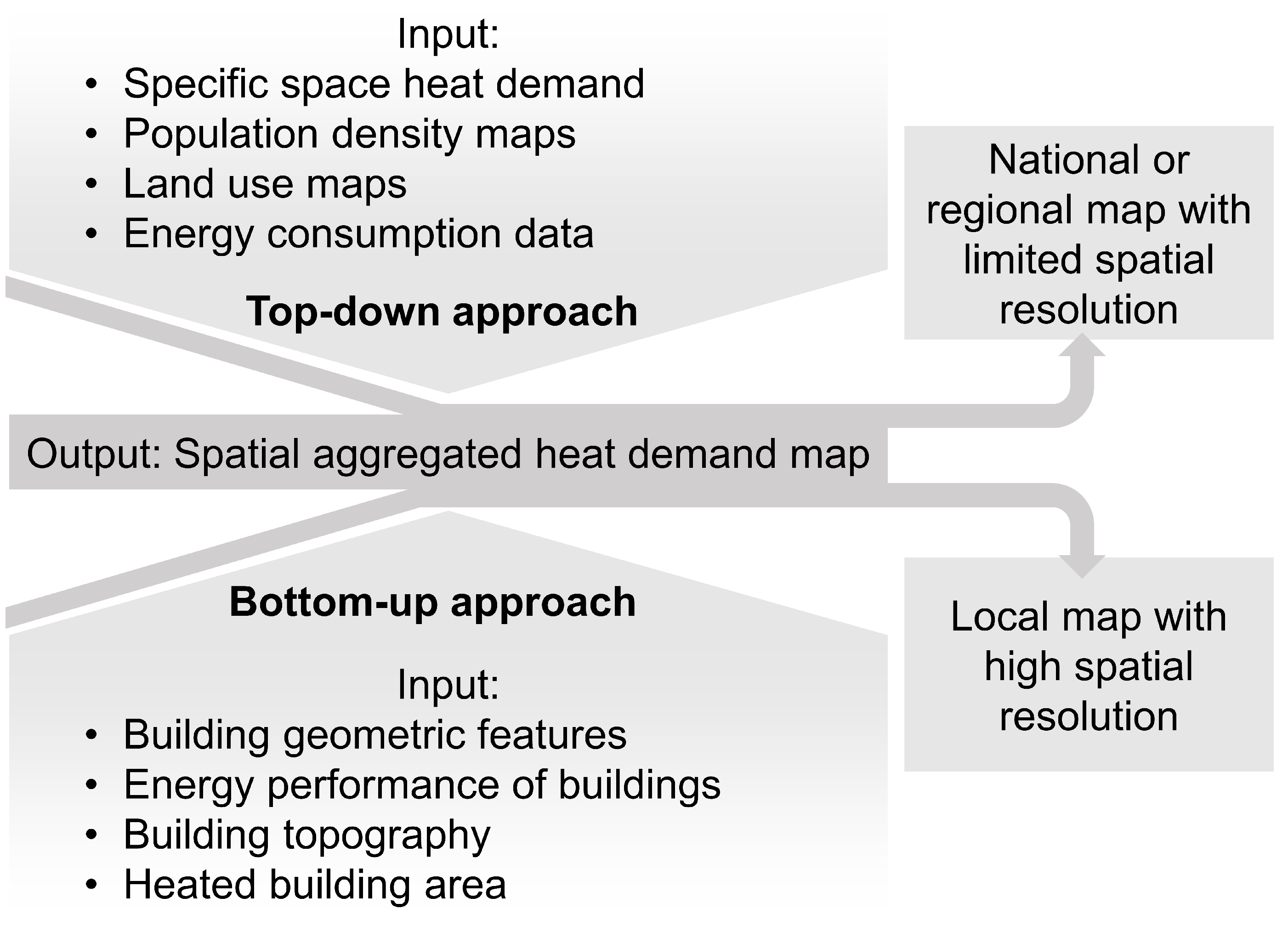
Figure 2.
The main steps from creating a coarse matrix to a fine matrix to calculating the final heat demand data.
Figure 2.
The main steps from creating a coarse matrix to a fine matrix to calculating the final heat demand data.

Figure 3.
The main steps of the methodology to process the provided HD polygons for the heat demand data categories 1 and 2.
Figure 3.
The main steps of the methodology to process the provided HD polygons for the heat demand data categories 1 and 2.
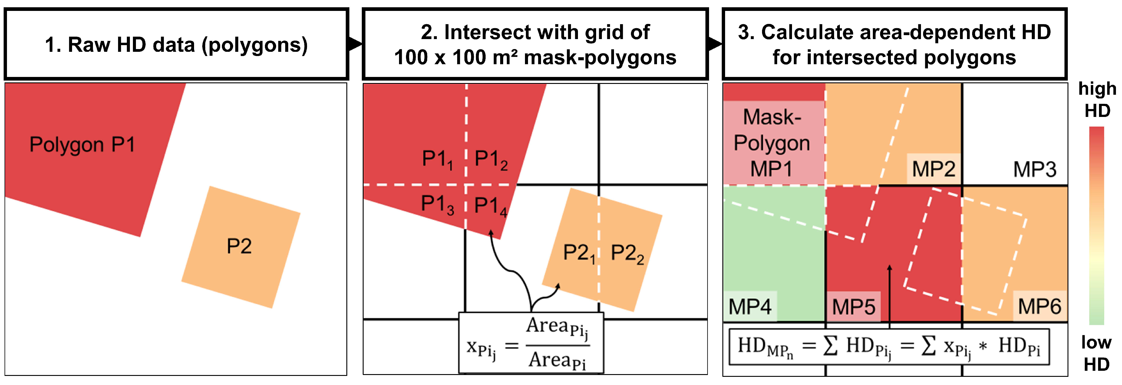
Figure 4.
The methodologies used for different heat demand input data. Top: Methodology used for heat demand categories 1, 2, and 4. For the methodology of heat demand category 3 (bottom), two input data types have been used: (a) the provided HD data with a low spatial resolution (point data per LAU) and (b) the Hotmaps data with a high spatial resolution (). The calculated scaling factor has been used to rescale the Hotmaps data for the DGE-ROLLOUT HD map.
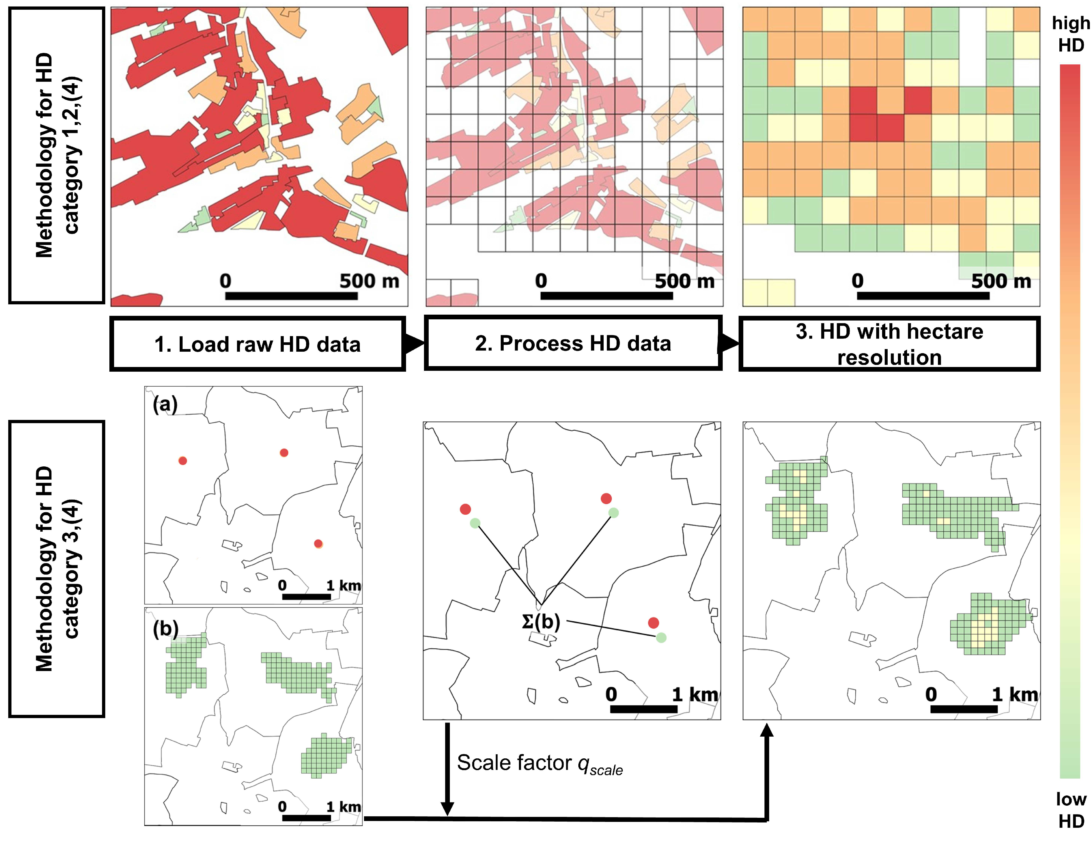
Figure 5.
The Interreg NWE region and the quality and spatial representation categories of each heat demand input data delivered by the responsible entities.
Figure 5.
The Interreg NWE region and the quality and spatial representation categories of each heat demand input data delivered by the responsible entities.
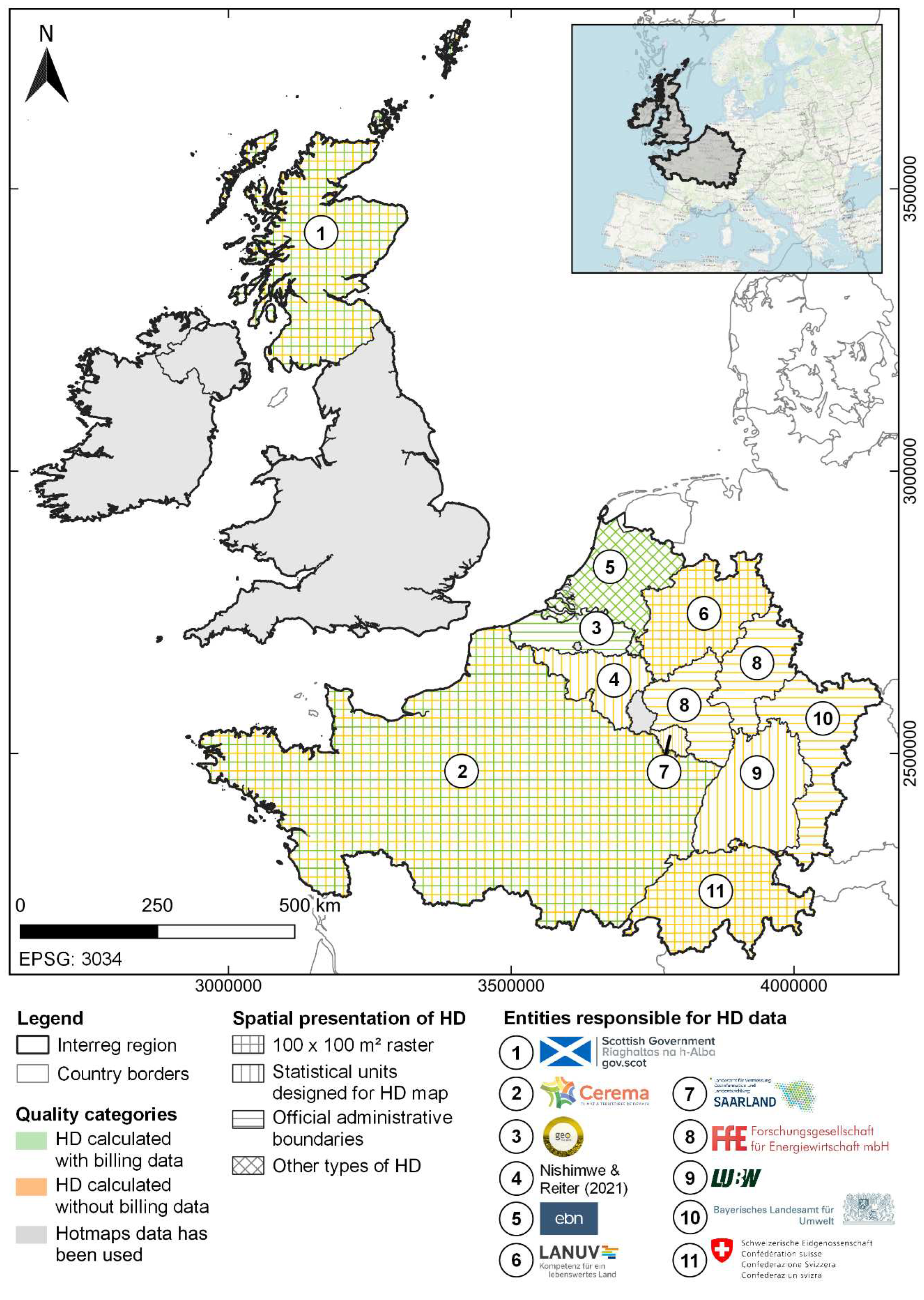
Figure 6.
The main steps of developing the heat demand difference maps.
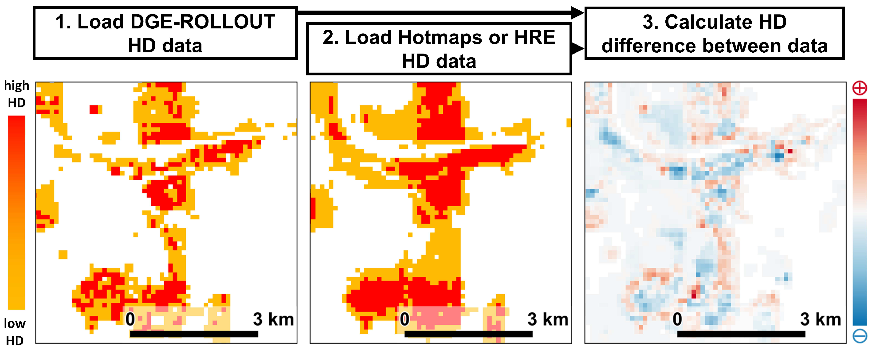
Figure 7.
Heat demand in MWh/ha per year of the Interreg NWE region for the residential and commercial sector and both sectors summed up (total HD). The legend applies to all three maps. There is no data with subclassification for the different sectors in Scotland, so it is not shown in the residential and commercial heat demand maps.
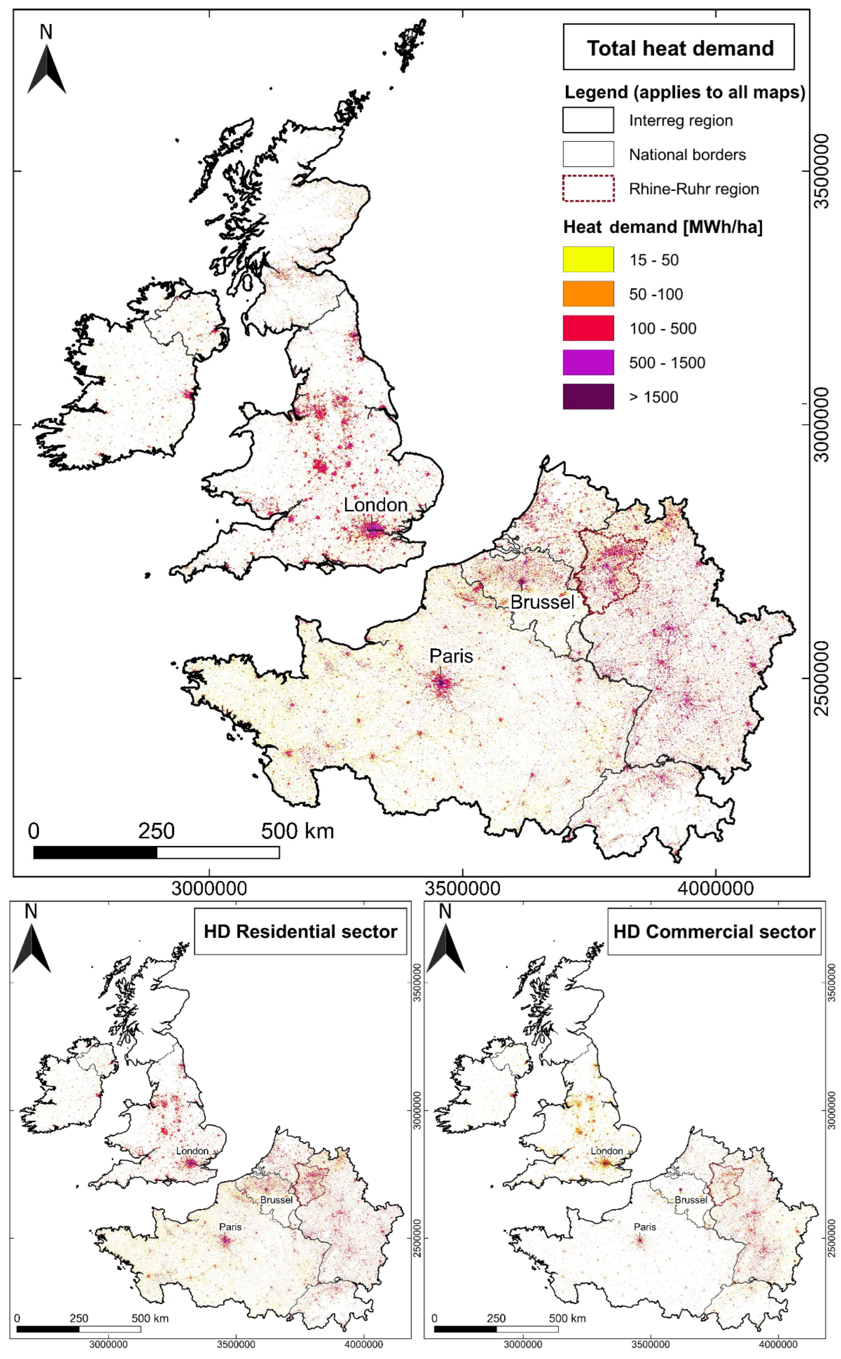
Figure 8.
(a) Country share of the total Interreg NWE heat demand. Share of the residential (b) and commercial (c) heat demand per country.
Figure 8.
(a) Country share of the total Interreg NWE heat demand. Share of the residential (b) and commercial (c) heat demand per country.
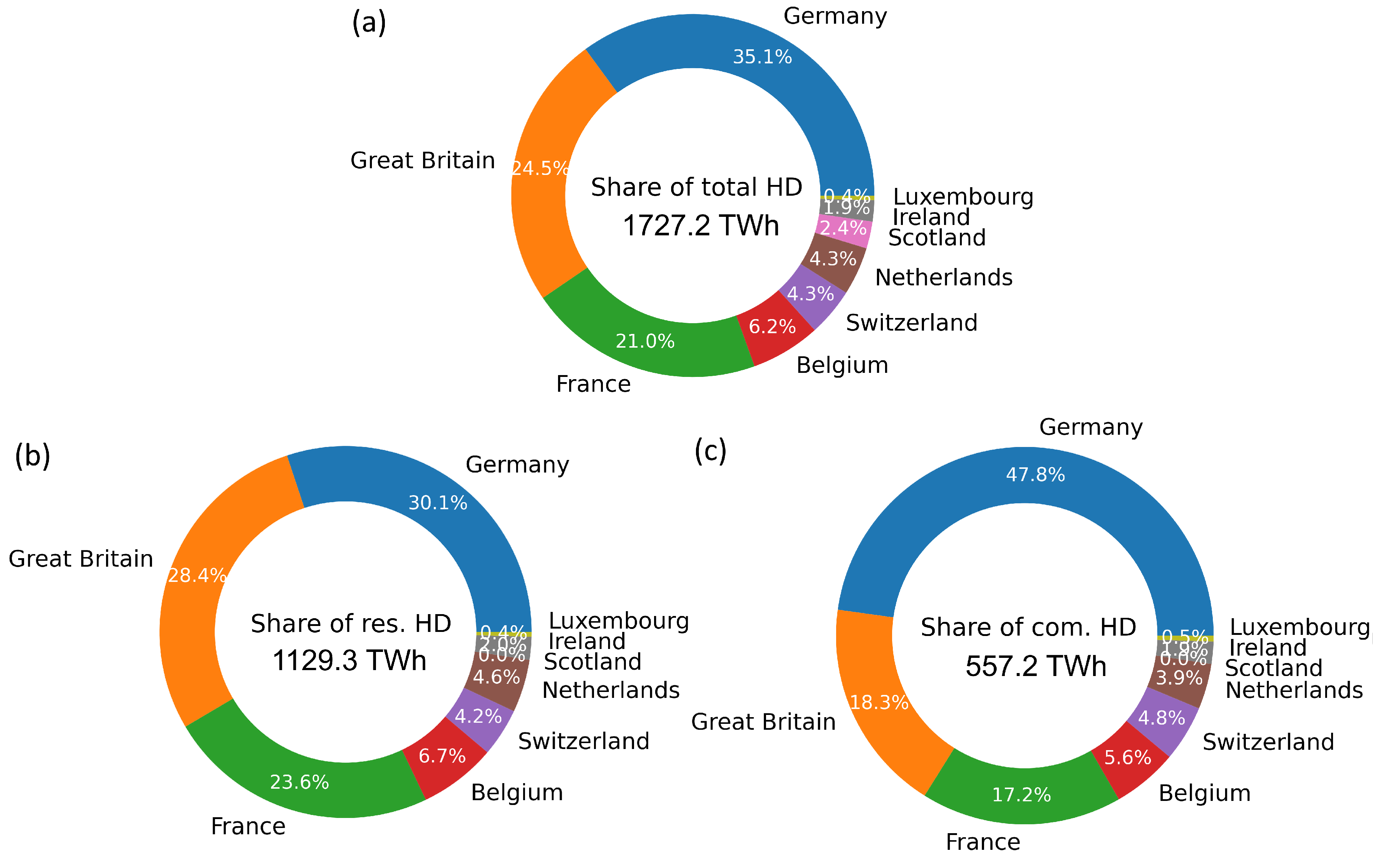
Figure 9.
Total Heat Demand [] for the different NUTS-1 regions. Values are sorted by total HD.
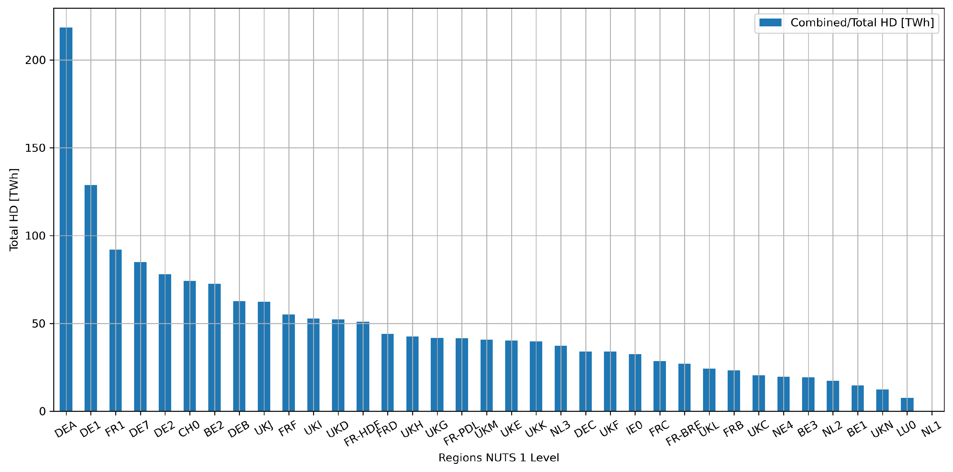
Figure 10.
Average of heated area of total HD [] for the different NUTS-1 regions. Values are sorted according to the total HD values shown in Figure 9.
Figure 10.
Average of heated area of total HD [] for the different NUTS-1 regions. Values are sorted according to the total HD values shown in Figure 9.
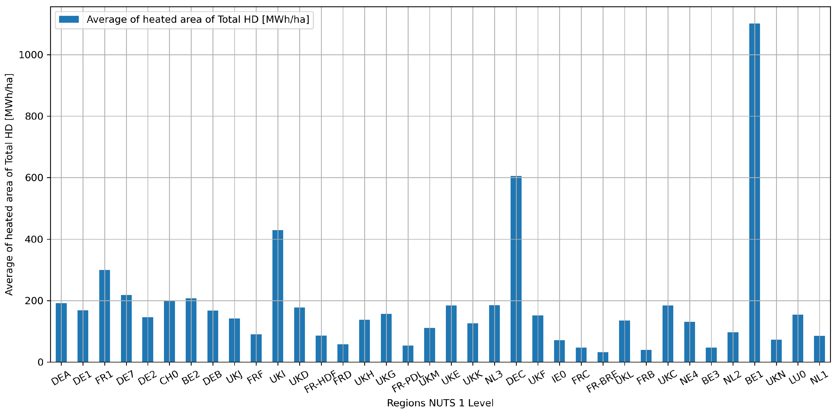
Figure 11.
Share of the residential and commercial sector in heat demand depending on the degree of urbanization in each country.
Figure 11.
Share of the residential and commercial sector in heat demand depending on the degree of urbanization in each country.
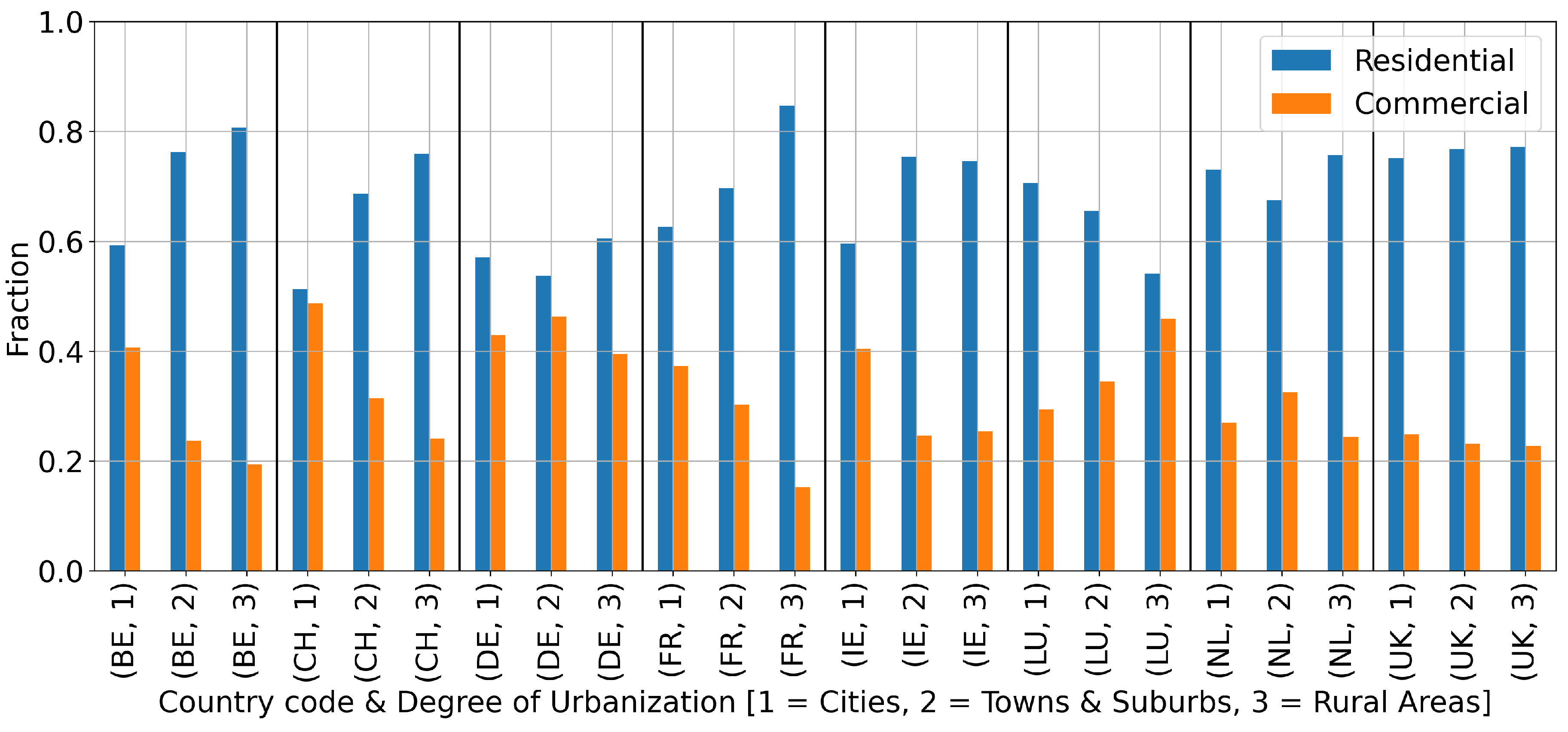
Figure 12.
Ratios between population per city and summed up total heat demand per area definition according to the urban areas of the OECD.
Figure 12.
Ratios between population per city and summed up total heat demand per area definition according to the urban areas of the OECD.
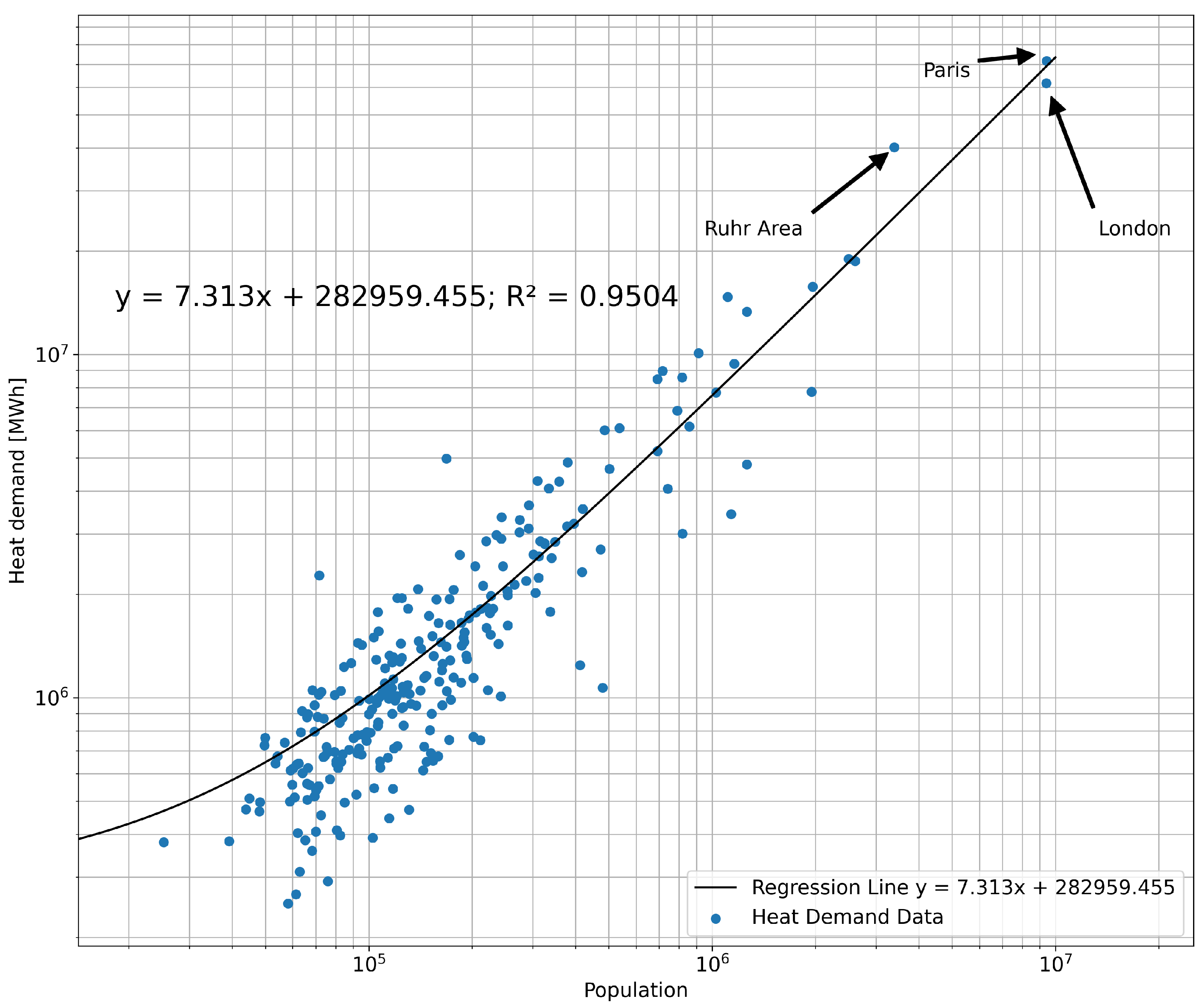
Figure 13.
The ratios between population per city and summed up total heat demand per hectare per area definition according to the urban areas of the OECD.
Figure 13.
The ratios between population per city and summed up total heat demand per hectare per area definition according to the urban areas of the OECD.
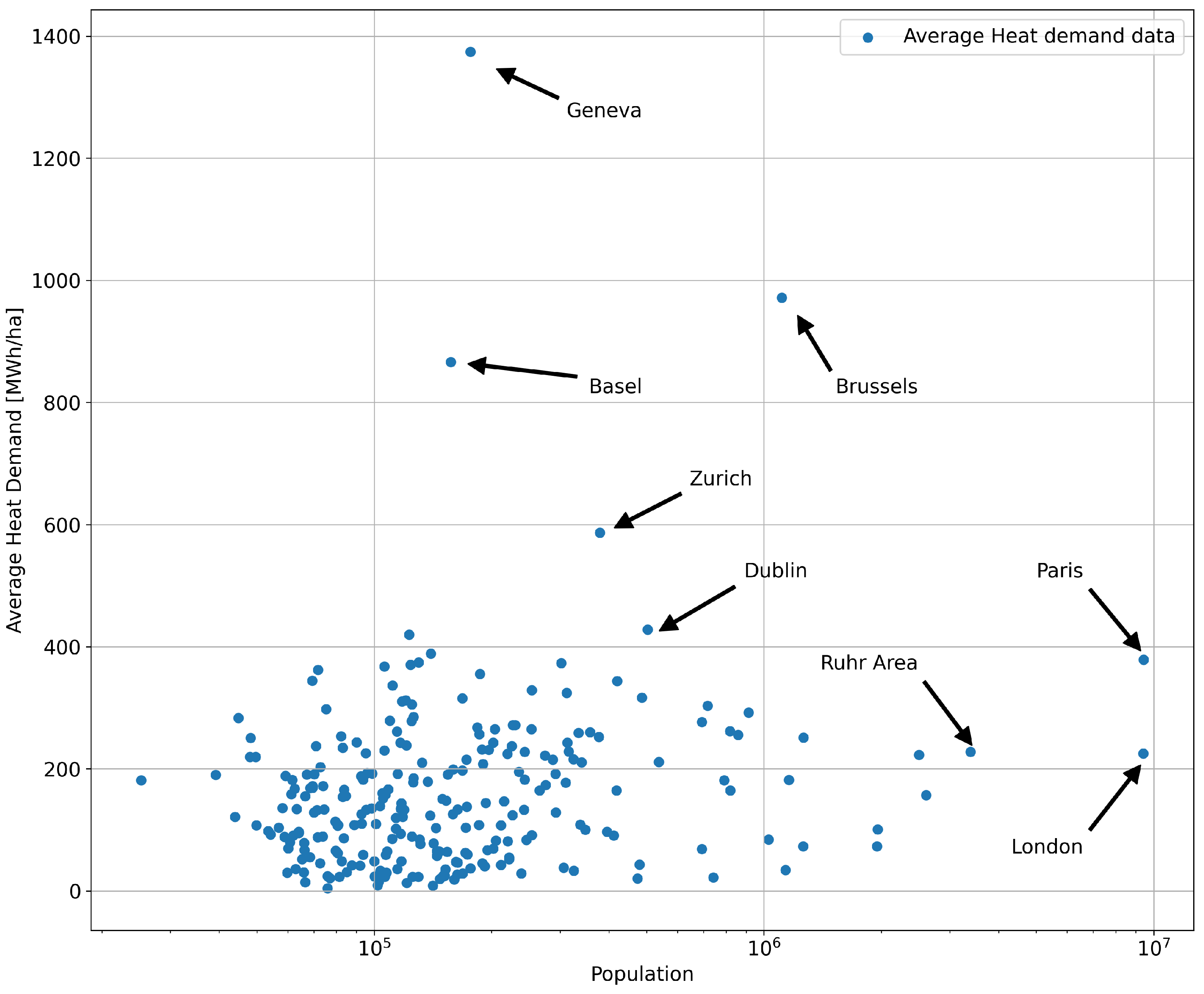
Figure 14.
Series of HD difference maps, where the Hotmaps and HRE HD maps were subtracted from the DGE-ROLLOUT HD map for each raster cell in the residential, the commercial sector, and in total. For IR, the UK without SCT and LUX HD, data from Hotmaps has been used in the DGE-ROLLOUT HD map.
Figure 14.
Series of HD difference maps, where the Hotmaps and HRE HD maps were subtracted from the DGE-ROLLOUT HD map for each raster cell in the residential, the commercial sector, and in total. For IR, the UK without SCT and LUX HD, data from Hotmaps has been used in the DGE-ROLLOUT HD map.
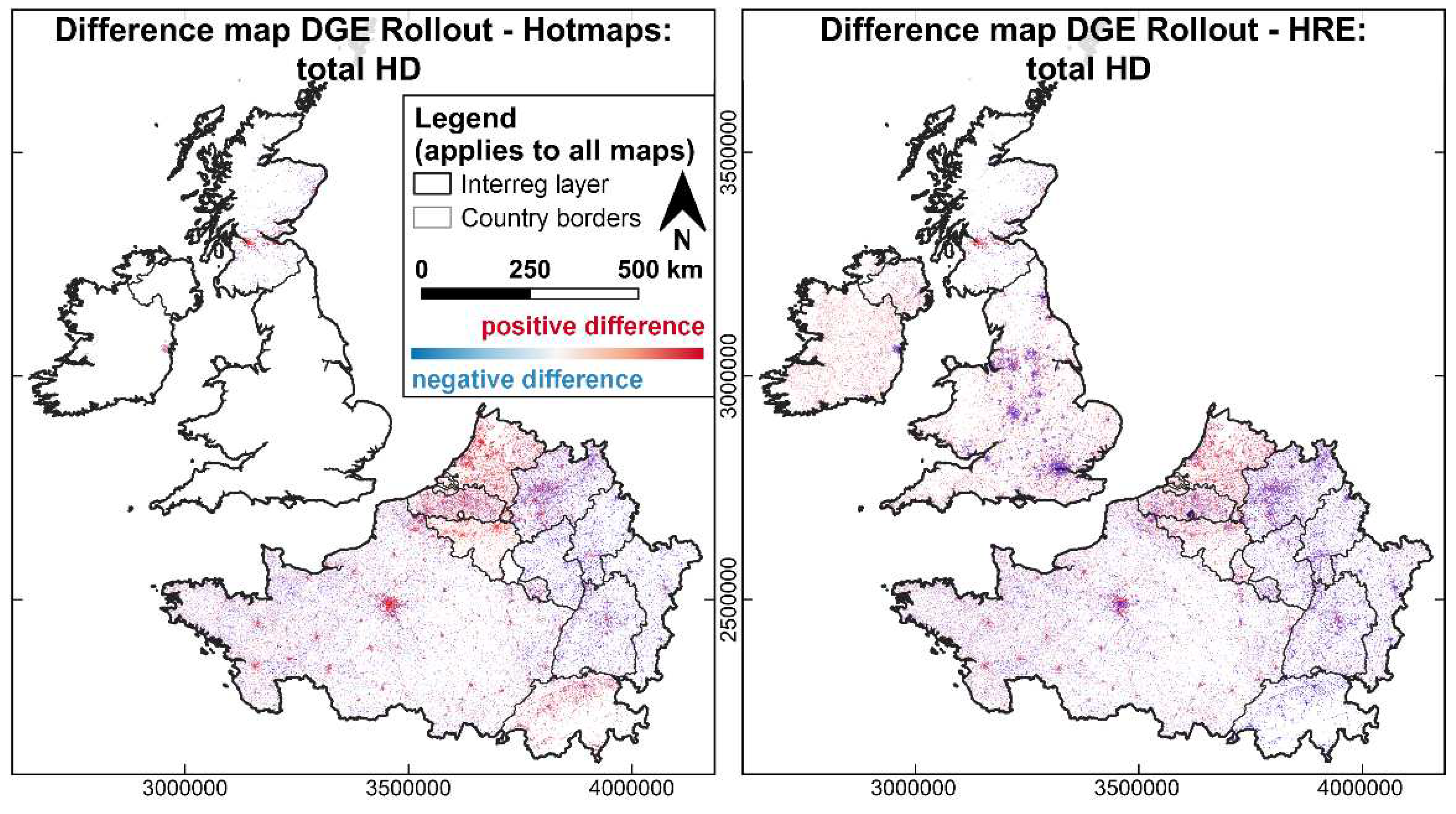
Figure 15.
Violin plots showing the statistical dispersion of mean values for the residential sector, commercial sector, and for total HD difference with Hotmaps and HRE in comparison. The pale envelope in the background displays the statistical dispersion of the standard mean error.
Figure 15.
Violin plots showing the statistical dispersion of mean values for the residential sector, commercial sector, and for total HD difference with Hotmaps and HRE in comparison. The pale envelope in the background displays the statistical dispersion of the standard mean error.
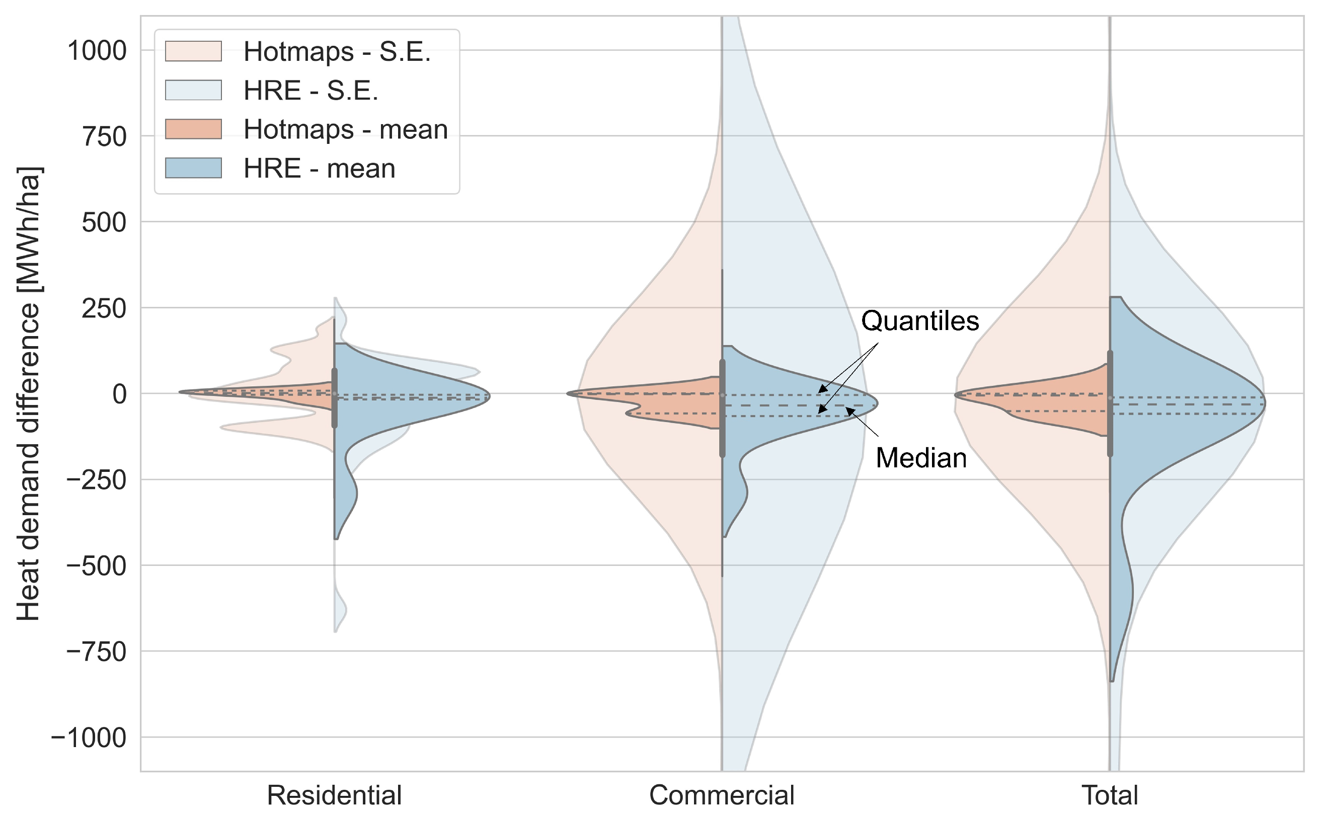
Figure 16.
The DGE-ROLLOUT HD map shown of the city of Aachen and the three-country border between BE-WAL (data category 4), DE-NW (data category 1), and NL (data category 4). Note, that NL is based on real consumption data, whereas the other HD data are based on a modeled top-down approach.
Figure 16.
The DGE-ROLLOUT HD map shown of the city of Aachen and the three-country border between BE-WAL (data category 4), DE-NW (data category 1), and NL (data category 4). Note, that NL is based on real consumption data, whereas the other HD data are based on a modeled top-down approach.
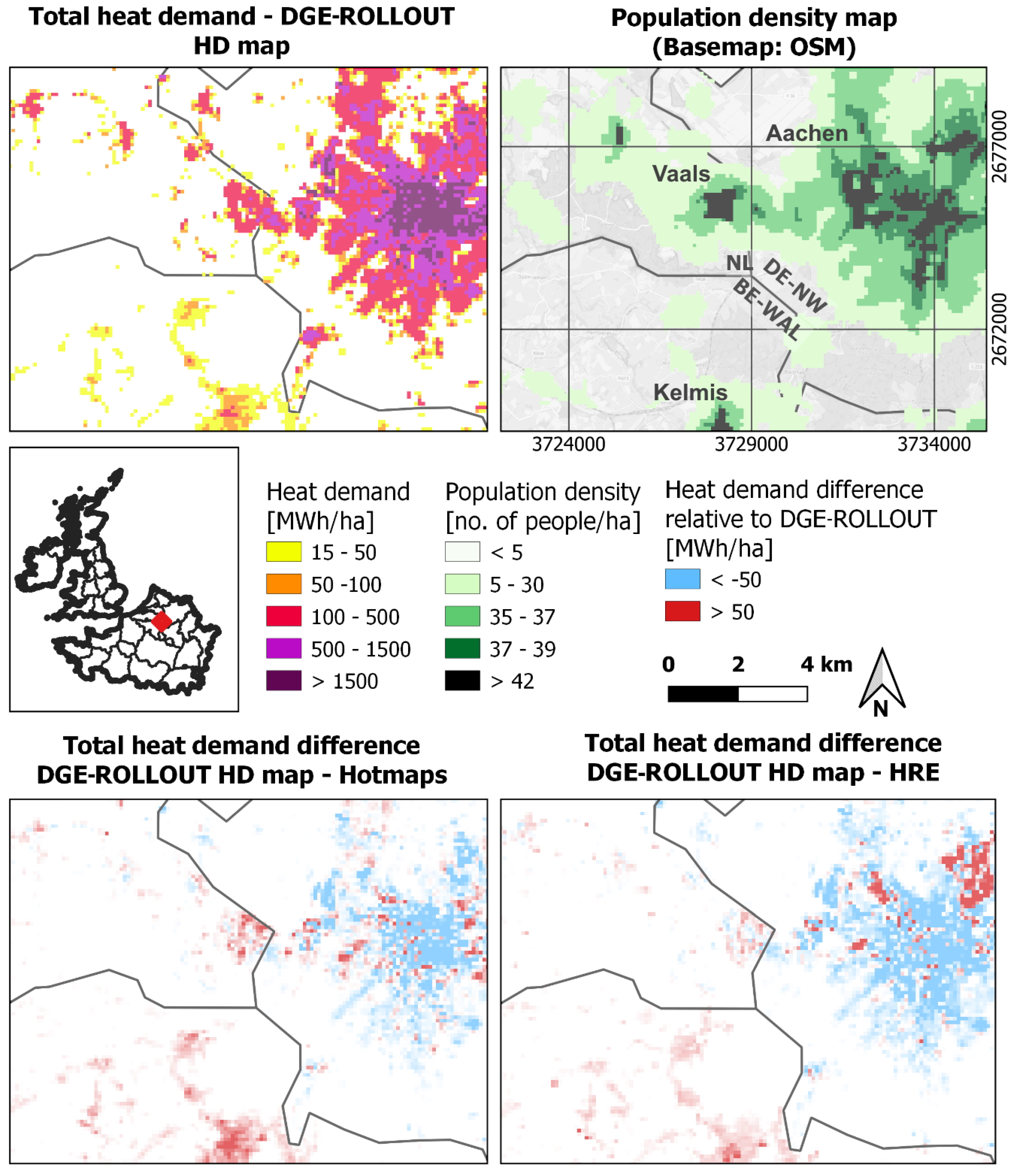
Table 1.
The different spatial categories of the provided heat demand data for the DGE-ROLLOUT project. The exact citation can be found in the references.
Table 1.
The different spatial categories of the provided heat demand data for the DGE-ROLLOUT project. The exact citation can be found in the references.
| Data category | Description | Regions (ISO 3166) and prev. studies |
| 1 | HD data provided as (e.g. ) raster or polygon grid with the same or in a different coordinate reference system | CH [12], FR [18,19], DE-NW [16], UK-SCT [22], Hotmaps [24], HRE [25] |
| 2 | HD data provided as building footprints or street segments | BE-VLG [11], DE-BW [13], DE-SL [17] including industrial parts |
| 3 | HD data provided as a point or polygon layer, which contains the sum of the HD for regions of official administrative units | DE-BY [15], DE-HE & DE-RP [14] |
| 4 | HD data provided in other data formats such as HD data associated with addresses | NL [20,21], BE-WAL [41] |
| 5 | No HD data available for the region | Luxembourg, United Kingdom excl. Scotland |
Disclaimer/Publisher’s Note: The statements, opinions and data contained in all publications are solely those of the individual author(s) and contributor(s) and not of MDPI and/or the editor(s). MDPI and/or the editor(s) disclaim responsibility for any injury to people or property resulting from any ideas, methods, instructions or products referred to in the content. |
© 2023 by the authors. Licensee MDPI, Basel, Switzerland. This article is an open access article distributed under the terms and conditions of the Creative Commons Attribution (CC BY) license (http://creativecommons.org/licenses/by/4.0/).
Copyright: This open access article is published under a Creative Commons CC BY 4.0 license, which permit the free download, distribution, and reuse, provided that the author and preprint are cited in any reuse.


