
Submitted:
19 February 2024
Posted:
20 February 2024
You are already at the latest version
Abstract
Eutrophication, a global concern, impacts water quality, ecosystems, and human health. It’s crucial to monitor algal blooms in freshwater reservoirs, as they indicate the trophic condition of a waterbody through Chlorophyll-a (Chla) concentration. Traditional monitoring methods, however, are expen-sive and time-consuming. Addressing this hindrance, we developed models using remotely sensed data from the Sentinel-2 satellite for large-scale coverage, including its bands and spectral indexes, to estimate the Chla concentration on 149 freshwater reservoirs in Ceará, Brazil. Several machine learning models were trained and tested, including k-nearest neighbours, random forests, extreme gradient boosting, the least absolute shrinkage, group method of data handling (GMDH), and sup-port vector machine models. A stepwise approach determined the best subset of input parameters. Using a 70/30 split for the training and testing datasets, the best-performing model was the GMDH, achieving an R2 of 0.91, MAPE of 102.34%, and RMSE of 20.38 g/L, which are values consistent with the ones found in the literature. Nevertheless, the predicted Chla concentration values were most sensitive to the red, green, and near infra-red bands.
Keywords:
Chlorophyll-a
; Sentinel-2 satellite
; Machine learning
; Freshwater Reservoirs
; Eutrophication
1. Introduction
Eutrophication, an essential manifestation of water pollution in freshwater reservoirs, results from the excessive nutrient loads that cause algal blooms [1,2]. The excessive algae and aquatic plant growth result in oxygen depletion, ultimately causing severe impacts on aquatic ecosystems and considerably increasing the costs related to water treatment [3,4,5,6].
Chlorophyll-a (Chla), a photosynthetic pigment in major algae groups, is widely used as a critical indicator of phytoplankton presence [7,8]. Because the abundance of algae can reflect the state of eutrophication, Chla is one of the most important parameters for evaluating the trophic condition of water bodies [9,10]. While Chla concentration has long served as a critical parameter in monitoring harmful blooms, accurately predicting Chla in reservoirs has proven to be a persistent challenge [11,12]. This difficulty is mainly due to the non-linear and non-stationary characteristics of Chla concentration, which are influenced by anthropogenic and hydrometeorological factors [2].
In regions characterized by semi-arid climates, such as Northeastern Brazil, establishing an extensive network of multi-purpose artificial reservoirs has emerged as a reliable solution to confront the water scarcity challenges imposed by environmental constraints [13,14]. These reservoirs are notably susceptible to eutrophication due to hydroclimatic characteristics that combined favor photosynthesis and biodegradation [15,16], such as interannual variability of precipitation and stored volume [17], high temperatures and evaporation rates [18], and prolonged hydraulic retention time [19]. Moreover, this susceptibility is further aggravated by continued anthropogenic pressure on water bodies due to internal enrichment from aquaculture practice [3,20], inadequate coverage of sanitation systems [21], and a dense reservoir network [22,23].
Therefore, regularly monitoring Chla concentrations is crucial for implementing effective water quality management strategies to prevent further deterioration [24]. However, traditional sampling methods are expensive, time-consuming, and impractical for many reservoirs [25,26]. As an attractive option, satellite remote sensing and machine learning (ML) techniques offer a cost-effective approach for monitoring Chla concentrations and their spatiotemporal variations, providing large-scale data on complex environmental systems [27]. The Sentinel-2 constellation has been proved to be a valuable asset in monitoring inland and coastal waters once it has improved spatial resolution compared to other freely available sensing systems data, such as Landsat 8 [28,29].
The ML approach retrieves complex non-linear relationships within satellite data, capturing the underlying structure bonding the satellite data and the desired target variable [30,31]. Combining ML architectures with remote sensing data has been able to provide top-notch results in a plethora of scientific fields, such as solar irradiance forecasting [32], mapping of mineral extraction sites [33], forest fire mapping [34], and crop water stress evaluation [35].
ML and satellite data performance has also been explored for Chla monitoring inland and ocean waters. For ocean water, including coastal waters, specific Chla ML forecasting models, namely OLCI Neural Network Swarm (ONNS) and Ocean Colour 4 for MERIS (OC4ME), using Sentinel-3 satellite data, showed good performance for such a task [36,37]. However, other possible ML paradigms can be found for inland and coastal waters. A random forest (RF) based model was developed in [38]. In their study, the authors used Sentinel-2 imagery to retrieve Chla concentrations for lake Chagan in China. Their proposed model provided good performance in determining the Chla concentrations and complyingwith the biological mechanism in lakes, offering robust results to seasonal changes.
In Cao et al. [9], the authors used Landsat-8 remote sensing data together with extreme gradient boosting tree model (XGBoost) ML to determine Chla in lakes located in China. Their approach was implemented to analyze the spatiotemporal data from 2013 to 2018, and it demonstrated satisfactory performance in identifying the Chla behavior in the study location. In Hu et al. [39], the authors developed methodologies to mitigate spectral noise in satellite data to improve the performance of ML models to estimate Chla in global oceans using remote sensing from several satellites. Their results proved that the support vector regression (SVR) was the best-performing ML approach, surpassing the traditional band-ratio models and providing reduced image noise.
The Group Method of Data Handling (GMDH) has also been applied to hydrological scenarios, including Chla estimation [40], water quality prediction [41], and image classification for plant diseases [42]. However, there is a gap in the knowledge regarding the usage of this approachin modeling Chla concentration using satellite data, which the present study aims to fulfill. Additionally, the present study seeks to provide a deep insight into the performance of ML paradigms when applied to a vast area containing heterogeneous reservoirs.
Given this scenario, the potential to increase algae blooms and further degradation of these aquatic systems has increased the need to study often poorly monitored reservoirs in semi-arid regions. Therefore, this study aims to estimate Chla concentration through combined remote sensing and machine learning techniques. For this, the following specific objectives were pursued in this research:
- A comprehensive investigation on several input parameters for Chla modeling, including all the 13 bands of the MSI onboard of Sentinel-2 constellation and 16 different spectral indexes.
- A comprehensive analysis and characterization of all the 149 tropical reservoirs extensively spread across the state of Ceará, located in the Brazilian semi-arid region.
- The usage of stepwise approach on parameters selection.
- The investigation of different machine learning paradigms for modeling Chla values in heterogeneous reservoirs distributed over a vast region.
- To fulfill the gap in the knowledge regarding the usage of the GMDH ML model for Chla modeling using remote sensed data and spectral indexes.
2. Materials and Methods
2.1. Study site location
The Brazilian semi-arid region is one of the most populated semi-arid regions in the world, with approximately 28 million inhabitants and an area that occupies 12% of the national territory [43]. The state of Ceará, inhabited by around nine million people, covers an area comparable in size to England of 150,000 km², where 98.6% of its territory is in the semi-arid region [44]. The region is characterized by extreme climatic events such as recurrent droughts, sporadic flooding and high inter-annual variability [45,46]. According to the Köppen classification [47], the climate is 'BSh', characterized by a mean precipitation of 750 mm per year, a potential evaporation rate of 2000 mm per year, a mean annual temperature of 31°C and negative water balances for most of the year [13,48]. Moreover, Ceará's state is influenced by two distinct seasons: a rainy season from January to April, when 80% of the total precipitation occurs, and a dry season during the rest of the year [49].
Since Ceará's water supply relies predominantly on artificial reservoirs, the state has a dense reservoir network, serving as the primary source for over 90% of the region’s water resources [20] and with a storage capacity of approximately 18.6 billion cubic meters. Notably, the three largest reservoirs in the state, Castanhão (6,700 hm³), Orós (1,940 hm³), and Banabuiú (1,600 hm³) collectively represent approximately 55% of the total storage capacity [50].
The study area includes data from 149 monitored reservoirs distributed across Ceará in twelve watersheds. The longitude, latitude, and basic information of the reservoirs are listed in Table S1 in the supplementary material. These reservoirs are mainly used for human water supply, aquaculture, fish farming, and irrigation. As a result, pollution is predominantly attributed to nonpoint sources such as livestock, agriculture, and soil erosion, and point sources originating from sewage and fish farming [51]. The trophic condition of these reservoirs fluctuates with seasonal changes and flooding or drought events [52]. Figure 1 illustrates the geographical location of Ceará within the Brazilian territory and in the semi-arid region, as well as the location of the reservoirs distributed across its area.
2.2. Water quality data
This study used data from 149 spatially distributed reservoirs (Figure 1), covering the years 2015 to 2021, including 1,399 Chla samples. This information was collected from the database provided by the Portal Hidrológico do Ceará platform, a system in which monitoring has been carried out by the Water Resources Management Company (COGERH) [50], a public agency maintained by the local government, presenting consistent time series of hydrological and water quality parameters. The company carries out monitoring campaigns in all seasons of the year through quarterly sampling campaigns and in situ measurements of parameters.
The Chla concentration data provided by the COGERH was obtained through in-situ water samples. The samples were gathered at each reservoir sampling point at 0.3 meters from the surface, collected into a dark flask to avoid exposure to light. Later, the sample’s pigments were extracted using a solution of 90% acetone to cold extract them. Finally, the pigments were used to assess the Chla concentration for each sample were analyzed by accredited laboratories according to a standardized protocol APHA 10200 H spectrometric method [13,53].
2.3. Sentinel-2 satellite data
2.3.1. Band data
The Sentinel-2 mission is an effort of the European Space Agency (ESA) to monitor the Earth’s environment. This mission comprises a constellation of two polar-orbiting satellites, namely Sentinel-2A and Sentinel-2B. Both satellites are placed in the same sun-synchronous orbit, aiming to monitor the Earth’s environmental changes [54,55]. The mission started with the launch of the first Sentinel-2A satellite in June 2015. The latter deployment of the second satellite, Sentinel-2B, in March 2017 reduced the revisiting time from 10 days to 5 days [56].
Besides the brief revisiting time, the Sentinel-2 mission is equipped with Multispectral Instruments (MSI), which provide information for different spatial resolutions, ranging from 10 m to 60 m, given the state-of-the-art anastigmatic telescope within it [55,57,58]. The MSI can register data from 13 spectral bands, varying from visible to near-infrared (NIR) and short-wave infrared (SWIR), providing high-resolution data for both inland and coastal areas [29,55,59].
The remote-sensed data used in the present work undergoes Level-1C processing. For this level of data processing the Earth’s spatial region is partitioned into tiles based on the UTM/WGS84 projection, with each tile separated by a distance of 100 km. Radiometric values for each tile’s pixel are determined for the top-of-atmosphere reflectances, which are later converted to radiance [60,61]. The quality of Level-1C processing is ensured by the ESA monthly, following rigorous quality standards [62].
The combination of reduced revisiting time, high spatial resolution, and wide range of spectral bands deem the Sentinel-2 an important mission with agriculture applications and forest monitoring [28]. Table 1 compiles the information for each spectral band.
Table 1 informs the wavelength for each band captured by the MSI. It is possible to notice that the wavelengths around 700 nm (NIR) suggest that the Sentinel-2 constellation is suited for capturing the phytoplankton spectral characteristics, including Chla, as the microscopic organisms cause a surge in spectral reflectance around the 700 nm mark [13,29,64].
Furthermore, given the satellite resolution, the water samples from the reservoirs were taken at a minimum distance of 60 meters from the shoreline. This precaution ensures that the pixel, corresponding to the smallest spatial resolution is entirely encompassed within the reservoir boundaries. Also, given the satellite revisiting time, most of the remotely sensed data had an interval of 1 to 2 days. Given that the Chla concentration does not vary significantly for the given period, this time-range is valid for our study application.
2.3.2. Satellite spectral indexes
Satellite spectral indexes are derived from mathematical equations combining two or more spectra of the satellite bands. These indices are a helpful approach to extracting information from the spectral bands pixelwise to model terrestrial processes and features, like vegetation, water, urban development, and agriculture [63,65,66]. A comprehensive investigation of 16 different indices and their impact on the model’s result was performed in the present study. Their mathematical formulations are displayed in equations 1 to 16.
In Equation 1, we have the normalized difference vegetation index (NDVI) formulation. This index is vastly used in remote sensing, being primarily used for the evaluation of green areas and the changes related to them. It is a valuable input on different remote sensing applications [67,68].
Equation 2 shows the formulation for the Green Normalized Difference Vegetation Index (GNDVI), an adapted version of the NDVI index aimed explicitly at detecting Chla in the vegetation [69,70].
The enhanced vegetation index (EVI) is similar to the previous NDVI but removes the impacts of the atmosphere and the soil over the vegetation signal [71,72].
The soil-adjusted vegetation index (SAVI) improves the NDVI index by considering the soil effects due to multiple scattering of soil [72,73].
The normalized difference moisture index (NDMI) is used to verify changes in vegetation physiology by determining its water content [74,75].
The moisture stress index (MSI) is used to evaluate changes in the water content in the vegetation via canopy stress analysis. It is also used to indicate water concentration in the soil [76,77].
The green chlorophyll vegetation Index (GCI), as its name implies, is applied to the remote sensed data to estimate chlorophyll concentration in the vegetation and, consequently, determine the health of the analyzed vegetation [78,79].
The normalized burned ratio index (NBRI) seeks to identify the occurrence and severity of natural or man-made fires in vegetation areas [80,81].
The bare soil index (BSI) formulated in Equation 9 retrieves information from the vegetation in cases where its coverage is less than half of the assessed area. This index allows us to determine the vegetation health concerning the exposed soil area [82,83].
The normalized difference water index (NDWI) retrieves information from water bodies effectively from remote sensing data [84,85].
The Normalized Difference Snow Index (NDSI) is a tool that detects snow cover in a specific area by analyzing the light reflection properties of ice. This index retrieves information by distinguishing snow coverage from other surfaces and adjusting for atmospheric and terrain effects [86,87,88].
The normalized difference glacier index (NDGI), similar to NDSI, identifies glacier coverage in a region mainly composed of snow, ice, and debris [89,90].
The atmospherically resistant vegetation index (ARVI) is an improvement over the NDVI index by implementing atmospheric corrections. The ARVI is especially useful for regions under dense aerosol coverage [91,92].
The structure-insensitive pigment index (SIPI) was initially proposed to identify vegetation stress via the ratio between carotenoid and chlorophyll in vegetation. It is also useful for analyzing vegetation structures with different canopy configurations [93,94].
The sentinel water mask (SWM) specifically seeks to detect water data from the Sentinel-2 constellation [95].
The automated water extraction index (AWEI) is used to accurately detect water given various environmental interferences [96,97].
A first analysis of the indexes may result in the conclusion that some of them, e.g., NDSI and NDGI, may not be suitable for the study location due to the semi-arid characterization of the Ceara state. However, a careful examination of Equations 11 and 12, together with Table 1, elucidates that the mentioned indexes result from bands within the spectral range that favour Chla identification and are of high spatial resolution [13,29,64]. Therefore, these indexes may still carry relevant spatiotemporal information that may help uncover the latent relationship between the input parameters and Chla, thus improving the performance of the ML models. This potential improvement provides a compelling reason for further investigation into the participation of these indices in Chla modeling. Figure 2 and Figure 3 show the correlation between the satellite bands and Chla and the indexes and Chla, respectively. In both images, the lighter the color, the more correlated the variables are.
Figure 2 shows that the bands share a significant correlation between themselves, but band 10. In contrast, in Figure 3, the indexes show less correlation with each other, indicating potential to be used by ML models due to their low collinearity. Regarding the correlation with the Chla attribute, the bands present significantly lower values, up to ten times smaller than the correlation between the indexes and Chla.
The elevated correlation within the bands’ data does not necessarily mean a positive impact on the performance of the forecasting model. Highly correlated variables, when used as inputs on a predictive model, may add noise to the dataset, increasing the model’s variance and thus reducing its performance [96,97]. However, discarding highly and low correlated variables altogether may also harm the model’s performance since they may still carry relevant spatiotemporal information relating to the inputs' and outputs' attributes, leading to improved forecasting performance [30].
2.4. Machine learning models
Chla was estimated using satellite data and machine learning models. The first implemented approach was the random forest (RF). The RF is a model composed of trees trained using the bagging method of resampling considering just a subset of predictors (Figure 2 and Figure 3) [100,101], deeming it an ensemble model. The trained trees are low correlated, reducing the ensemble model variance and improving performance [98,99,100]. Different published works have investigated the RF methodology [101,102,103].
XGBoost [104] was also implemented as a standalone model and used as benchmark for the models' performance. This tree-based approach is an ensemble model and an extreme improvement over the random forest. It consists of bag sampling smaller tree models, which are combined into a larger and more robust tree-model, reducing the model variance while improving its generalization and reducing the model's tendency to overfit [98,105]. The XGBoost model can handle missing data and manipulate increasing dataset size, keeping its generalization. This approach reached excellent results when applied to different time-series forecasting tasks [106,107,108].
Another ML used in Chla prediction in this work was the k-nearest neighbors (k-NN). The k-NN algorithm is a supervised ML model, which uses non-parametric vectors to determine an unknow point [109]. However, given that it is also based on the distance between points distributed on a possible multi-dimensional space, a distance metric must be implemented, often the Euclidean distance [109,110,111]. The k-NN architecture can be applied to data classification and regression model cases [109,112]. For the former application, the model classifies an unknow datapoint considering its neighbors by a simple voting system, assigning the unknow point the label of the most common class around it. The latter approach has a similar implementation, but this time, a continuous value is assigned to an unknow point given the average value of the target attribute of its neighbors [109,112,113]. Despite its simplicity, the regression performed by the k-NN approach offers competitive results within the ML field and has been explored for different scenarios in previous studies [114,115,116].
The Support Vector Machine (SVM) was also implemented in this study. The SVM is a flexible ML approach with diverse applications for classification, regression, and outlier detection [117]. Initially proposed by Cortes and Vapnik in 1995 [118], with previous formulations dating back to the 1960s, the SVM is a generalization of the maximal margin classifier [112]. The SVM learns a boundary function discriminating the dataset when implemented for classification. At the same time, regression provides a best-fitting function describing the data behavior by taking into consideration its extreme attribute vectors. A unique feature of SVM is the use of kernel functions that allow the dataset to be manipulated into higher-dimensional spaces, making it possible for the model to learn complex non-linear relationships by applying convex optimization without being computationally expensive, reducing the training error [109,119,120]. However, one drawback of the SVM approach is that it does not handle large datasets efficiently, requiring extended computational time to be trained [121,122].
The least absolute shrinkage and selection operator (LASSO) regression [123] was another implemented ML methodology. This approach is a more straightforward ML methodology, which seeks to implement the best linear regression line in the dataset. Besides that, the LASSO paradigm is also a regularization and parameter selection approach, making its results more interpretable than other traditional ML models [98,123].
Lastly, using satellite data, we investigated the GMDH ML model for the Chla modeling. It was first proposed by Ivakhnenko [124] as an alternative to address the challenges of linear dependency and equation complexity for higher dimensional problems and small data sequences [40,125]. This methodology is a feedforward unidirectional ML model, similar to a multilayer perceptron [126,127]. It is also a self-organizing model, indicating that its parameters are selected automatically, not needing parameter tuning [128]. The resulting value by the GMDH model is a quadratic approximation, using pair combinations of the input variables [129,130], which are used to model the relationship between input and the output parameters [131]. Unlike other artificial neural network paradigms, the GMDH does not need vast training data, as the estimation of its parameters is automatically determined without recursion [40]. The performance of the GMDH model was verified in previous studies for time-series challenges, including hydrological applications [132,133,134].
2.5. Evaluation metrics
To assess the forecasts by the proposed models, we opted to calculate the metrics root mean squared error (RMSE), normalized RMSE (nRMSE), mean absolute error (MAE), mean absolute percentage error (MAPE), mean bias error (MBE), and coefficient of determination (R2). Their equations can be verified in [135] for R2, and [136] for the remaining metrics.
2.6. Dataset preprocessing and attribute selection.
The dataset standardization seeks to restrain the dataset to within the same dimensionless scale, setting the mean value equal to zero and the standard deviation to one, often improving the model’s performance [32]. Besides the data standardization, in this study, the Yeo-Johnson transformation [137] was implemented for some of the ML models. This transformation is an improvement over the Box-Cox approach, which is restricted to handling positive numbers only. The Yeo-Johnson transformation is based on the power transformation with different parameters to positive and negative values and is presented in Equation 18 [137].
Where the transformed value ψ is a function of the original attribute value, , and a parameter , which is determined via maximum likelihood [101,102]. This transformation seeks to reduce the data skewness, approximating the original dataset distribution to a normal distribution as [138,139].
The best parameters were selected among the bands and indexes. To this end, using a step-by-step approach [112], we started investigating the influence of the bands only. First, we investigated the performance of just one band at a time, from band 1 to 12, and we selected the best one that returned the best R2, using the XGBoost model as the benchmarking approach. After that, we tested the combination of the already selected bands, with the remaining ones, again, one by one, and kept the band that returned the highest coefficient of determination value (forward variable selection). This process was repeated until all the bands were investigated and their best combination was kept [112].
The same procedure was repeated for the selection of the indexes. This time, we started the investigation with the best band selection previously set. Then, we added one index at a time to the input parameters, selecting the index which yielded the highest R2. Again, the process was repeated until all the indexes were assessed. The selection of the best bands and indexes are presented in Figure 4 and Figure 5, respectively.
As depicted in Figure 4, the modeling for Chla substantially improved with the combination of bands 6, 4, 10, 7, 8a, 9, 5, 12, and 3, resulting in an R2 of 0.36. Figure 5 shows that the addition of the indexes also managed to increase the coefficient of determination to 0.50 after including NBRI, NDSI, AWEI, SAVI, NDVI, MSI, GCI, GNDVI, and ARVI in the selected input data. Interestingly, the NDSI, an index related to snow coverage, promoted improvements over the Chla identification, as indicated in Figure 5, proving that it conveyed spatiotemporal information for the modeling approach. Therefore, the results discussed in the subsequent section are based on grouping the aforementioned spectral bands and indexes.
3. Results
3.1. Limnological behavior
The mean value for Chlorophyll varied widely among reservoirs and according to seasonality. Considering the complete dataset, Chla values ranged from a minimum of 1 μg/L to a maximum of 1001.78 μg/L, with a mean value of 39.62 μg/L and a standard deviation of 65.78 μg/L. The boxplot in Figure 6-A shows the inter-annual and intra-annual distribution of the dataset. Mean values decreased throughout the years (from 81.34 μg/L in 2015 to 27.84 μg/L in 2021), while maximum values did not reflect this tendency, with recorded values increasing, for example, from 707.06 in 2015 to 1001.78 in 2016, indicating the occurrence of concentration blooms. Regarding the intra-annual distribution of Chla, higher concentrations were detected in the rainy seasons for most of the studied years, except in 2017.
The state’s three largest reservoirs were also analyzed (Figure 7-B). The mean recorded values for Orós were the highest (31.89 μg/L), between 9.20 and 60.94 μg/L, while Chla for Banabuiú was found in lower mean concentrations (21.64 μg/L) between 1.82 and 54.55 μg/L. For Castanhão, values ranged from 5.65 and 78.72 μg/L with mean Chla value of 29.03 μg/L.
3.2. Results for Chla estimation by the ML models
The proposed models were built using the variables presented in Figure 4 and Figure 5 as input parameters. We used data from the Sentinel-2 satellite and on-site measurements from the 149 reservoirs to train and test these models. We adopted a 70/30 split for the training and validation datasets. These datasets were randomly assembled using data spanning from 2015 to 2021. It is important to notice that given the random separation for the training and validation data, not all the reservoirs may have been included in the validation dataset. However, this does not mean that the validation dataset is not significant and statistical characteristics similar to the training dataset.
The hyperparameters of the used ML models, except for the GMDH self-organizing approach, were selected using the GridSearch tool for Scikit-Learn, with 5-fold cross-validation [140,141]. The outcomes for Chla modeling by each one of the assessed models are presented in Table 2.
Table 2 shows that the ML approaches reached similar results regarding the RMSE metric, but for the GMDH, which surpassed all of the assessed paradigms, achieving RMSE of 20.38 μg/L. The LASSO model achieved the highest error value for RMSE, with 89.87 μg/L, followed by the k-NN model, with RMSE value of 61.82 μg/L. The tree-based models XGBoost and RF achieved similar RMSE values of 55.60 μg/L and 56.75 μg/L, respectively. The SVR output scored an RMSE value equal to 50.64 μg/L. It is essential to disclose that an analysis of the RMSE alone may be misleading to assess the performance of the models. The coefficient of determination is another crucial factor to consider in this scenario. This parameter indicates the total variance of the dependent variable Chla, which can be adequately forecasted by the input parameters and may be understood as an indication of the accuracy achieved by the model [142]. This behavior can be better visualized in Figure 7.
Figure 7 shows how the predicted data compares with the actual measured Chla values. We used log values to facilitate the comparison due to differences in the variables’ scales. The histograms showcase the normal distribution of the data after the logarithm transformation. In Figure 7, given the log scale, minor fluctuations in Chla values correspond to negligible alterations in the satellite-captured data. This is not related to the used GMDH model itself but is a consequence of the chosen scale. In fact, the remote sensed data lacks the sensibility to convey sufficient information for low Chla values, since the main characteristics of high Chla concentrations are their tendency to converge to a specific spectral pattern of green, while for low values they tend to converge to different spectral patterns that depend on the characteristics of each reservoir.
Still in Figure 7, it is possible to observe that both predicted and real data present similar distributions, which indicates the GMDH model's good performance in predicting Chla levels. The regression line displayed in the plotting area shows a positive correlation between the predicted and real Chla data, further attesting to the robust GMDH performance. The points clustered around the regression line also indicate the superior performance of the GMDH algorithm, especially for extreme values as depicted by the top-rightmost points in the graph area. Comparing the results in Table 2, we can observe that the highest R² value reached by the GMDH model was 0.91, representing a significant improvement of 57% over the SVR result, the second best-performing approach regarding the same parameter. The third- and fourth-best performing models were the tree-based ones XGBoost and RF, which achieved R² equal to 0.50 and 0.48, respectively. The k-NN performance, R2 equal to 0.38, and the LASSO model, R2, equal to 0.38, achieving a coefficient of determination equal to 0.41, was the worst-performing modeling paradigms. Analysis on the values of MAE and MAPE indicates that the GMDH is able to output more accurate and precise results when compared to the others assessed models. The negative values for MBE is a trend presented in all the investigated paradigms. It indicates that the ML models share the tendency to underestimate the outputs for Chla value.
4. Discussion of the results
Mainly in tropical regions, the mechanisms that regulate phytoplankton growth require an advanced analysis due to the complexity and nonlinearity of the relationship between chlorophyll and physicochemical/environmental factors [13,143]. The approach presented in this study achieves this analysis using a highly heterogeneous collection of in-situ observations, investigating the performance of different ML models to determine Chla levels in 149 dams in the Brazilian state of Ceará. Although most dams were predominantly eutrophic throughout the years, different human activities and pollution sources have contributed to eutrophication processes lead to Chla spatiotemporal fluctuations and algal blooms [17,20,144,145].
We applied the forward stepwise approach to select the parameters, including bands and spectral indexes. To our knowledge, this method has not yet been applied in previous remote sensing studies. The forward stepwise approach s, significantly improving the Chla determination for the ML models. Existing literature regarding the influence of spectral bands on Chla determination can be found. In work [146], the authors applied the SHAP analysis to explain the influence of the Sentinel-2 spectral bands for estimating Chla values. Their results elucidated that band 3, band 2, and band 8 were the top three most influential parameters for Chla determination. Bands 3 and 2 exhibited a positive correlation with the Chla, while band 8 showed a relevant negative correlation with the same parameter. A similar approach was conducted by Kim et al. [147]. In their work, the SHAP analysis showed relevant participation in Chla prediction of red bands, i.e., bands 4, 5, and 6, and blue and green bands (Table 1), a similar conclusion found by Ha et al. [148].
The influence of different spectral indexes for Chla modeling was investigated in previous works. Castro et al. [149] showed that indexes merging red and NIR bands yielded the best outcomes for determining Chla concentrations in small reservoirs. Similar conclusions were drawn by Buma and Lee [150] and by Aubriot et al. [151], which attested to the importance of bands within the red spectral range for Chla characterization in a lake in Chad, and for the Rio de La Plata, respectively. On the other hand, Viso-Vazquez et al. [152], showed that the green band, i.e., band 3, promoted the highest correlation between the remote sensing data and Chla levels.
Our results show the GMDH methodology could efficiently identify the latent non-linear ties ruling input and output attributes. Moreover, the GMDH approach proved to be a more robust model for analyzing satellite imagery, being more resilient to noises and satisfactory results when handling different band information, which also can be attributed to its improved performance.
To better understand where the GMDH results lie within the literature, we compared our results with those found in previously published works. Such evaluation, however, may not be representative given the different methodologies used in different studies, models, input attributes, and the study area. Yet, comparing their evaluation metrics is still a viable approach to assess the performance of different models [153]. Table 4 compiles the results for the GMDH model, while Table 5 gathers the results found in the literature.
Table 5 shows that the models based on the deep learning methodology all performed remarkably well in determining Chla levels. Compared to the results found in our study, it is possible to notice that the R-squared values for references [154,155] are in the same range, over 90%. Nevertheless, regarding the work by Guo et al. [154], the combined utilization of Sentinel-2 and Landsat-8 data significantly enhances the machine learning model's performance. This improvement is primarily due to the reduction in the revisit time, which subsequently minimizes the variance in the dataset. Consequently, this leads to a more robust and accurate machine-learning model. It is important to note that, although their results are slightly superior, the study location is limited to only one place.
Adding more water bodies is expected to add variance to the dataset. The model in reference [156] was built using modeled data, including 11 times more water bodies than the previous studies. Their results proved to be slightly inferior to the other two previous works and more relatable to the ones found in this present assessment, with RMSE in the same magnitude order.
Regarding the R2, our GMDH model showed a nearly 10% superior value. However, it must be stated that since the data used for training the ML model was simulated, it may not consider several naturally occurring situations. This would lead to a more homogeneous dataset with less variance, improving the ML model performance compared to the model proposed in our study. Another significant difference is the time window used for testing the developed model in reference [156], which is significantly smaller than the one used in our model [160], which reduces the dataset variance, improving the ML performance.
The DL approaches presented in Table 5 still require a considerable amount of data to yield reliable outputs. Depending on the data availability for the study location, this characteristic may pose a major drawback. On the other hand, the GMDH paradigm can be promptly implemented with less information available and does not require extensive training datasets [40], deeming them more flexible for different situations.
References [157,158] applied SVR to determine Chla. It is noticeable that although the models are the same, their methodology was disparate. Regarding reference [157], the RMSE values were within the same order of magnitude. Besides that, the R2 values were relatively close to each other. Contrarywise, reference [158] performed a much broader study regarding several lakes spread across the Chinese territory. As previously mentioned, the inclusion of different lakes allows the forecasting model to generalize its results better, and thus provide more robust outcomes. Another critical difference between these two works is that the former implemented as input information just the spectral bands of the MSI onboard of Sentinel-2, while the latter used both bands and indexes. In this aspect, the present study achieved superior performance, attesting the GMDH model benefited from the inclusion of spectral indexes, which improved their Chla outcomes.
The work conducted by Aranha et al. [13] shares the same location as the one used in this study. However, they used only a subset of 5 reservoirs of 149. In their approach, the authors fitted a regression line to their dataset using the three-band spectral index (3BSI), showing a good agreement between the index and the Chla values. A similar methodology was implemented in reference [152], where the Toming’s index was used to fit a regression line for Chla values. These two studies implemented spectral bands to estimate Chla concentrations. By evaluating the R2 metric values for [13,152], the proposed GMDH was superior over both studies, with significant improvements of 12% and 5%, respectively. Furthermore, a major difference between these two studies and the methodology presented in this work, is the data handling. The other studies used methodologies of fitting a regression line using the proposed indexes over the entire dataset, making no distinction between training and testing datasets. This is analogous to assessing our ML model's performance considering the training dataset only. Therefore, their methodologies lack generalization, being bound to a particular time and geographic location. In addition, while these approaches are considerably less complex than the proposed ML model, they provide valuable insights into Chla's behavior when analyzed using the evaluated indexes.
In the work conducted by Pompêo et al. [159], the Sentinel Application Platform (SNAP) algorithm was evaluated for modeling the Secchi disk depth, the Chla concentration and the number of Cyanobacteria cells. The study location was the Cantareira System (CS) in the Brazilian state of São Paulo, Brazil. In their study, authors used in situ collected water samples from 6 reservoirs in the CS as ground truth for the evaluated water quality parameters. These data were latter compared with the Case 2 Regional Coast Color (C2RCC) atmospheric correction algorithm. It is a machine learning paradigm based on neural networks trained to reproduce top-of-atmosphere reflectance [161]. The results of their study showed a good correlation between the modeled data and the real collected samples for the Chla, achieving an RMSE value of 2.3 μg/L and R2 of 0.75.
A direct comparison of these results with the ones found in our study shows an R-squared value 16% superior for the GMDH approach, while the C2RCC had better RMSE values. The reasoning behind this discrepancy for the error metric is twofold. Firstly, even though both studies were conducted in Brazilian territory, the state of São Paulo is characterized with having a subtropical and tropical climate type [162]. Such climatic configuration is much less prone to dry seasons compared to the studied semi-arid region of the Ceará state. This consistency leads to less fluctuation in Chla levels. Consequently, this could decrease the model’s variance, thus enhancing the model’s performance. Secondly, the work presented by Pompêo et al. used significantly fewer reservoirs compared to the present work. As previously mentioned, the reduced number of reservoirs hinders the model capacity to generalize unknown data while diminishing the dataset's variance, leading to improved error outcomes. However, despite improved error, the C2RCC model is a less robust approach when compared to the GMDH algorithm, as evidenced by comparing the R2 metric of both models.
It is important to disclose that our study was conducted in a tropical semi-arid region, considering 149 dams, considerably larger than any of the presented literature. In addition, a broader investigation of the spectral indexes for the Sentinel-2 constellation was assessed compared to the references in Table 5. This allows us to gather further insight into the impact of the spatiotemporal influence of both bands and indexes on the Chla prediction. From the results for parameter selection in Figure 4 and Figure 5, we observe that bands 8 and 11 do not compose the selected bands set. However, they are still present in the form of indexes. Moreover, a careful assessment of the GMDH results (available at Supplementary Spreadsheet 1) showcases the relevant contribution of bands 3, 4, 5, 7, 8, and 11 to the Chla prediction. This indicates that the predictive models benefit from a higher spatial resolution, as well as from green, red and infra-red bands composing the indexes, according to the literature [13,29,64].
5. Conclusions
This study evaluated several input parameters for Chla modeling in a vast spatial coverage of 149 freshwater reservoirs spanning a semi-arid tropical region across the Brazilian state of Ceará. This evaluation was conducted based on satellite remotely sensed data and ground-truth Chla concentration measurements that reflected the temporal and spatial distribution, notably impacted by interannual rainfall variability. To this end, we investigated the performance of several ML approaches, namely the k-nearest neighbours, random forests, extreme gradient boosting, the least absolute shrinkage and selection operator, support vector machine, and GMDH.
Forward stepwise parameter selection was implemented to determine the best input attribute selection among the 13 bands from the Sentinel-2 constellation and 16 spectral indexes derived from such bands. The usage of this methodology applied to the remote sensing field is, to the best knowledge of the authors, new and proven to improve the outcomes of the investigated Chla forecasting models. Figure 7 elucidates the performance of the GMDH model, showing that the model under investigation yielded excellent values for the Chla concentrations, achieving R2 value greater than 90%.
It is important to emphasize that our methodology ensures a clear separation between training and testing data, unlike some studies found in the literature. The approach is substantial for applying ML models, as a way to promote more robust results and capacity to generalize unseen data. This approach is especially crucial for a large dataset such as the one used in the present work, comprising 149 reservoirs in a semi-arid region similar in size to England, where the spatiotemporal variation of the data is substantial. Regarding the spectral bands and indexes, we showed that the Chla modeling benefited primarily from red, NIR, and green bands.
Extensive comparison with the literature found studies showed that the used models in this work offer competitive results. It is important to note that such a comparison may be misleading due to the disparate methodologies and study locations, directly influencing the ML outcomes.
In future works, the addition of more indexes, as well as the merge of Sentinel-2 data with Landsat-8 could be investigated. Including more spectral indexes and the Landsat-8 MODIS data would provide more spatiotemporal information and reduce data variance due to the finer temporal resolution. Furthermore, implementing atmosphere correction preprocessing could also benefit the predictive paradigms, as it would reduce data noise, diminish the error variance, and improve the forecasting of Chla concentration.
Supplementary Materials
The following supporting information can be downloaded at the website of this paper posted on Preprints.org.
Author Contributions
Conceptualization, I.E.L.N. and P.A.C.R.; methodology, I.E.L.N., P.A.C.R., F.A.S.F., J.V.G.T., and B.G.; software, P.A.C.R.; validation, I.E.L.N., P.A.C.R., F.A.S.F., J.V.G.T., and B.G.; formal analysis, I.E.L.N. and P.A.C.R.; investigation, I.E.L.N., P.A.C.R., F.A.S.F., J.V.G.T., and B.G.; resources, I.E.L.N. and P.A.C.R.; data curation, I.E.L.N. and P.A.C.R.; writing—original draft preparation, B.M.D.M.G., V.O.S., I.E.L.N. and P.A.C.R.; writing—review and editing, B.M.D.M.G., V.O.S., I.E.L.N., F.A.S.F., J.V.G.T., and B.G.; visualization, B.M.D.M.G., V.O.S., I.E.L.N. and P.A.C.R.; supervision, I.E.L.N., P.A.C.R., J.V.G.T. and B.G.; project administration, I.E.L.N., P.A.C.R., J.V.G.T. and B.G.; funding acquisition, B.G. and J.V.G.T. All authors have read and agreed to the published version of the manuscript.
Funding
This research study was funded by the Natural Sciences and Engineering Research Council of Canada (NSERC) Alliance, grant No. 401643, in association with Lakes Environmental Software Inc., and by the Conselho Nacional de Desenvolvimento Científico e Tecnológico—Brasil (CNPq), grant no. 303585/2022-6 and grant no. 312308/2020-5, and by Coordenação de Aperfeiçoamento de Pessoal de Nível Superior—Brasil (CAPES), grant no. PROEX 04/2021.
Data Availability Statement
Publicly available datasets were analyzed in this study. This data can be found here: https://drive.google.com/drive/folders/1ALvoqdtj1nbfdNWmna0PpJnD1xUgzLqw (accessed on 20 December 2023).
Conflicts of Interest
The authors declare no conflict of interest.
References
- Mamun, M.; Kwon, S.; Kim, J.-E.; An, K.-G. Evaluation of Algal Chlorophyll and Nutrient Relations and the N:P Ratios along with Trophic Status and Light Regime in 60 Korea Reservoirs. Science of The Total Environment 2020, 741, 140451. [Google Scholar] [CrossRef] [PubMed]
- Zhang, X.; Chen, X.; Zheng, G.; Cao, G. Improved Prediction of Chlorophyll-a Concentrations in Reservoirs by GRU Neural Network Based on Particle Swarm Algorithm Optimized Variational Modal Decomposition. Environmental Research 2023, 221, 115259. [Google Scholar] [CrossRef]
- Rocha, M.D.J.D.; Lima Neto, I.E. Internal Phosphorus Loading and Its Driving Factors in the Dry Period of Brazilian Semiarid Reservoirs. Journal of Environmental Management 2022, 312, 114983. [Google Scholar] [CrossRef] [PubMed]
- Rodríguez-López, L.; Usta, D.B.; Duran-Llacer, I.; Alvarez, L.B.; Yépez, S.; Bourrel, L.; Frappart, F.; Urrutia, R. Estimation of Water Quality Parameters through a Combination of Deep Learning and Remote Sensing Techniques in a Lake in Southern Chile. Remote Sensing 2023, 15, 4157. [Google Scholar] [CrossRef]
- Rolim, S.B.A.; Veettil, B.K.; Vieiro, A.P.; Kessler, A.B.; Gonzatti, C. Remote Sensing for Mapping Algal Blooms in Freshwater Lakes: A Review. Environ Sci Pollut Res 2023, 30, 19602–19616. [Google Scholar] [CrossRef] [PubMed]
- Rocha, P.A.C.; Santos, V.O.; Thé, J.V.G.; Gharabaghi, B. New Graph-Based and Transformer Deep Learning Models for River Dissolved Oxygen Forecasting. 2023. [CrossRef]
- Kayastha, P.; Dzialowski, A.R.; Stoodley, S.H.; Wagner, K.L.; Mansaray, A.S. Effect of Time Window on Satellite and Ground-Based Data for Estimating Chlorophyll-a in Reservoirs. Remote Sensing 2022, 14, 846. [Google Scholar] [CrossRef]
- Zhu, W.-D.; Qian, C.-Y.; He, N.-Y.; Kong, Y.-X.; Zou, Z.-Y.; Li, Y.-W. Research on Chlorophyll-a Concentration Retrieval Based on BP Neural Network Model—Case Study of Dianshan Lake, China. Sustainability 2022, 14, 8894. [Google Scholar] [CrossRef]
- Cao, Z.; Ma, R.; Duan, H.; Pahlevan, N.; Melack, J.; Shen, M.; Xue, K. A Machine Learning Approach to Estimate Chlorophyll-a from Landsat-8 Measurements in Inland Lakes. Remote Sensing of Environment 2020, 248, 111974. [Google Scholar] [CrossRef]
- Fu, L.; Zhou, Y.; Liu, G.; Song, K.; Tao, H.; Zhao, F.; Li, S.; Shi, S.; Shang, Y. Retrieval of Chla Concentrations in Lake Xingkai Using OLCI Images. Remote Sensing 2023, 15, 3809. [Google Scholar] [CrossRef]
- Dzurume, T.; Dube, T.; Shoko, C. Remotely Sensed Data for Estimating Chlorophyll-a Concentration in Wetlands Located in the Limpopo Transboundary River Basin, South Africa. Physics and Chemistry of the Earth, Parts A/B/C 2022, 127, 103193. [Google Scholar] [CrossRef]
- Karimian, H.; Huang, J.; Chen, Y.; Wang, Z.; Huang, J. A Novel Framework to Predict Chlorophyll-a Concentrations in Water Bodies through Multi-Source Big Data and Machine Learning Algorithms. Environ Sci Pollut Res 2023, 30, 79402–79422. [Google Scholar] [CrossRef]
- Aranha, T.R.B.T.; Martinez, J.-M.; Souza, E.P.; Barros, M.U.G.; Martins, E.S.P.R. Remote Analysis of the Chlorophyll-a Concentration Using Sentinel-2 MSI Images in a Semiarid Environment in Northeastern Brazil. Water 2022, 14, 451. [Google Scholar] [CrossRef]
- Barros, M.U.G.; Wilson, A.E.; Leitão, J.I.R.; Pereira, S.P.; Buley, R.P.; Fernandez-Figueroa, E.G.; Capelo-Neto, J. Environmental Factors Associated with Toxic Cyanobacterial Blooms across 20 Drinking Water Reservoirs in a Semi-Arid Region of Brazil. Harmful Algae 2019, 86, 128–137. [Google Scholar] [CrossRef] [PubMed]
- Lu, K.; Gao, X.; Yang, F.; Gao, H.; Yan, X.; Yu, H. Driving Mechanism of Water Replenishment on DOM Composition and Eutrophic Status Changes of Lake in Arid and Semi-Arid Regions of Loess Area. Science of The Total Environment 2023, 899, 165609. [Google Scholar] [CrossRef]
- Raulino, J.B.S.; Silveira, C.S.; Lima Neto, I.E. Assessment of Climate Change Impacts on Hydrology and Water Quality of Large Semi-Arid Reservoirs in Brazil. Hydrological Sciences Journal 2021, 66, 1321–1336. [Google Scholar] [CrossRef]
- Guimarães, B.M.D.M.; Neto, I.E.L. Chlorophyll-a Prediction in Tropical Reservoirs as a Function of Hydroclimatic Variability and Water Quality. Environ Sci Pollut Res 2023, 30, 91028–91045. [Google Scholar] [CrossRef] [PubMed]
- Rocha Junior, C.A.N.D.; Costa, M.R.A.D.; Menezes, R.F.; Attayde, J.L.; Becker, V. Water Volume Reduction Increases Eutrophication Risk in Tropical Semi-Arid Reservoirs. Acta Limnol. Bras. 2018, 30. [Google Scholar] [CrossRef]
- Rocha, M.D.J.D.; Lima Neto, I.E. Modeling Flow-Related Phosphorus Inputs to Tropical Semiarid Reservoirs. Journal of Environmental Management 2021, 295, 113123. [Google Scholar] [CrossRef] [PubMed]
- Wiegand, M.C.; Do Nascimento, A.T.P.; Costa, A.C.; Lima Neto, I.E. Trophic State Changes of Semi-Arid Reservoirs as a Function of the Hydro-Climatic Variability. Journal of Arid Environments 2021, 184, 104321. [Google Scholar] [CrossRef]
- Freire, L.L.; Costa, A.C.; Neto, I.E.L. Effects of Rainfall and Land Use on Nutrient Responses in Rivers in the Brazilian Semiarid Region. Environ Monit Assess 2023, 195, 652. [Google Scholar] [CrossRef]
- Rabelo, U.P.; Dietrich, J.; Costa, A.C.; Simshäuser, M.N.; Scholz, F.E.; Nguyen, V.T.; Lima Neto, I.E. Representing a Dense Network of Ponds and Reservoirs in a Semi-Distributed Dryland Catchment Model. Journal of Hydrology 2021, 603, 127103. [Google Scholar] [CrossRef]
- Rabelo, U.P.; Costa, A.C.; Dietrich, J.; Fallah-Mehdipour, E.; Van Oel, P.; Lima Neto, I.E. Impact of Dense Networks of Reservoirs on Streamflows at Dryland Catchments. Sustainability 2022, 14, 14117. [Google Scholar] [CrossRef]
- Li, J.; Pei, Y.; Zhao, S.; Xiao, R.; Sang, X.; Zhang, C. A Review of Remote Sensing for Environmental Monitoring in China. Remote Sensing 2020, 12, 1130. [Google Scholar] [CrossRef]
- Pahlevan, N.; Smith, B.; Schalles, J.; Binding, C.; Cao, Z.; Ma, R.; Alikas, K.; Kangro, K.; Gurlin, D.; Hà, N.; et al. Seamless Retrievals of Chlorophyll-a from Sentinel-2 (MSI) and Sentinel-3 (OLCI) in Inland and Coastal Waters: A Machine-Learning Approach. Remote Sensing of Environment 2020, 240, 111604. [Google Scholar] [CrossRef]
- Song, K.; Wang, Q.; Liu, G.; Jacinthe, P.-A.; Li, S.; Tao, H.; Du, Y.; Wen, Z.; Wang, X.; Guo, W.; et al. A Unified Model for High Resolution Mapping of Global Lake (>1 Ha) Clarity Using Landsat Imagery Data. Science of The Total Environment 2022, 810, 151188. [Google Scholar] [CrossRef] [PubMed]
- Shi, J.; Shen, Q.; Yao, Y.; Li, J.; Chen, F.; Wang, R.; Xu, W.; Gao, Z.; Wang, L.; Zhou, Y. Estimation of Chlorophyll-a Concentrations in Small Water Bodies: Comparison of Fused Gaofen-6 and Sentinel-2 Sensors. Remote Sensing 2022, 14, 229. [Google Scholar] [CrossRef]
- Segarra, J.; Buchaillot, M.L.; Araus, J.L.; Kefauver, S.C. Remote Sensing for Precision Agriculture: Sentinel-2 Improved Features and Applications. Agronomy 2020, 10, 641. [Google Scholar] [CrossRef]
- Bramich, J.; Bolch, C.J.S.; Fischer, A. Improved Red-Edge Chlorophyll-a Detection for Sentinel 2. Ecological Indicators 2021, 120, 106876. [Google Scholar] [CrossRef]
- Oliveira Santos, V.; Costa Rocha, P.A.; Thé, J.V.G.; Gharabaghi, B. Graph-Based Deep Learning Model for Forecasting Chloride Concentration in Urban Streams to Protect Salt-Vulnerable Areas. Environments 2023, 10, 157. [Google Scholar] [CrossRef]
- Oliveira Santos, V.; Costa Rocha, P.A.; Scott, J.; Van Griensven Thé, J.; Gharabaghi, B. Spatiotemporal Air Pollution Forecasting in Houston-TX: A Case Study for Ozone Using Deep Graph Neural Networks. Atmosphere 2023, 14, 308. [Google Scholar] [CrossRef]
- Rocha, P.A.C.; Santos, V.O. Global Horizontal and Direct Normal Solar Irradiance Modeling by the Machine Learning Methods XGBoost and Deep Neural Networks with CNN-LSTM Layers: A Case Study Using the GOES-16 Satellite Imagery. Int J Energy Environ Eng 2022, 13, 1271–1286. [Google Scholar] [CrossRef]
- Shirmard, H.; Farahbakhsh, E.; Müller, R.D.; Chandra, R. A Review of Machine Learning in Processing Remote Sensing Data for Mineral Exploration. Remote Sensing of Environment 2022, 268, 112750. [Google Scholar] [CrossRef]
- Mohajane, M.; Costache, R.; Karimi, F.; Bao Pham, Q.; Essahlaoui, A.; Nguyen, H.; Laneve, G.; Oudija, F. Application of Remote Sensing and Machine Learning Algorithms for Forest Fire Mapping in a Mediterranean Area. Ecological Indicators 2021, 129, 107869. [Google Scholar] [CrossRef]
- Virnodkar, S.S.; Pachghare, V.K.; Patil, V.C.; Jha, S.K. Remote Sensing and Machine Learning for Crop Water Stress Determination in Various Crops: A Critical Review. Precision Agric 2020, 21, 1121–1155. [Google Scholar] [CrossRef]
- Hieronymi, M.; Müller, D.; Doerffer, R. The OLCI Neural Network Swarm (ONNS): A Bio-Geo-Optical Algorithm for Open Ocean and Coastal Waters. Front. Mar. Sci. 2017, 4, 140. [Google Scholar] [CrossRef]
- Moutzouris-Sidiris, I.; Topouzelis, K. Assessment of Chlorophyll-a Concentration from Sentinel-3 Satellite Images at the Mediterranean Sea Using CMEMS Open Source in Situ Data. Open Geosciences 2021, 13, 85–97. [Google Scholar] [CrossRef]
- Shi, X.; Gu, L.; Jiang, T.; Zheng, X.; Dong, W.; Tao, Z. Retrieval of Chlorophyll-a Concentrations Using Sentinel-2 MSI Imagery in Lake Chagan Based on Assessments with Machine Learning Models. Remote Sensing 2022, 14, 4924. [Google Scholar] [CrossRef]
- Hu, C.; Feng, L.; Guan, Q. A Machine Learning Approach to Estimate Surface Chlorophyll a Concentrations in Global Oceans From Satellite Measurements. IEEE Trans. Geosci. Remote Sensing 2021, 59, 4590–4607. [Google Scholar] [CrossRef]
- Alizamir, M.; Heddam, S.; Kim, S.; Mehr, A.D. On the Implementation of a Novel Data-Intelligence Model Based on Extreme Learning Machine Optimized by Bat Algorithm for Estimating Daily Chlorophyll-a Concentration: Case Studies of River and Lake in USA. Journal of Cleaner Production 2021, 285, 124868. [Google Scholar] [CrossRef]
- Loc, H.H.; Do, Q.H.; Cokro, A.A.; Irvine, K.N. Deep Neural Network Analyses of Water Quality Time Series Associated with Water Sensitive Urban Design (WSUD) Features. Journal of Applied Water Engineering and Research 2020, 8, 313–332. [Google Scholar] [CrossRef]
- Chen, J.; Yin, H.; Zhang, D. A Self-Adaptive Classification Method for Plant Disease Detection Using GMDH-Logistic Model. Sustainable Computing: Informatics and Systems 2020, 28, 100415. [Google Scholar] [CrossRef]
- INSA O Semiárido Brasileiro. Available online: https://www.gov.br/insa/pt-br/semiarido-brasileiro/o-semiarido-brasileiro (accessed on 1 December 2023).
- IBGE Ceará | Cidades e Estados | IBGE. Available online: https://www.ibge.gov.br/cidades-e-estados/ce.html (accessed on 1 December 2023).
- Alvalá, R.C.S.; Cunha, A.P.M.A.; Brito, S.S.B.; Seluchi, M.E.; Marengo, J.A.; Moraes, O.L.L.; Carvalho, M.A. Drought Monitoring in the Brazilian Semiarid Region. An. Acad. Bras. Ciênc. 2019, 91, e20170209. [Google Scholar] [CrossRef]
- Pontes Filho, J.D.; Souza Filho, F.D.A.; Martins, E.S.P.R.; Studart, T.M.D.C. Copula-Based Multivariate Frequency Analysis of the 2012–2018 Drought in Northeast Brazil. Water 2020, 12, 834. [Google Scholar] [CrossRef]
- Beck, H.E.; Zimmermann, N.E.; McVicar, T.R.; Vergopolan, N.; Berg, A.; Wood, E.F. Present and Future Köppen-Geiger Climate Classification Maps at 1-Km Resolution. Sci Data 2018, 5, 180214. [Google Scholar] [CrossRef] [PubMed]
- Sacramento, E.M. do; Carvalho, P.C.M.; de Araújo, J.C.; Riffel, D.B.; Corrêa, R.M. da C.; Pinheiro Neto, J.S. Scenarios for Use of Floating Photovoltaic Plants in Brazilian Reservoirs. IET Renewable Power Generation 2015, 9, 1019–1024. [Google Scholar] [CrossRef]
- Raulino, J.B.S.; Silveira, C.S.; E.L. Neto, I. Eutrophication Risk Assessment of a Large Reservoir in the Brazilian Semiarid Region under Climate Change Scenarios. An. Acad. Bras. Ciênc. 2022, 94, e20201689. [Google Scholar] [CrossRef] [PubMed]
- COGERH Portal Hidrológico Do Ceará. Available online: http://www.hidro.ce.gov.br/ (accessed on 1 December 2023).
- COGERH Matriz Dos Usos Mútiplos Dos Açudes. Available online: http://www.hidro.ce.gov.br/hidro-ce-zend/mi/midia/show/149 (accessed on 1 December 2023).
- COGERH Qualidade Das Águas Dos Açudes Monitorados Pela COGERH.
- Standard Methods for the Examination of Water and Wastewater, 22nd ed.; American public health association, American water works association, Water environment federation, Eds.; American public health association: Washington (D.C.), 2012; ISBN 978-0-87553-013-0. [Google Scholar]
- Phiri, D.; Simwanda, M.; Salekin, S.; Nyirenda, V.; Murayama, Y.; Ranagalage, M. Sentinel-2 Data for Land Cover/Use Mapping: A Review. Remote Sensing 2020, 12, 2291. [Google Scholar] [CrossRef]
- Drusch, M.; Del Bello, U.; Carlier, S.; Colin, O.; Fernandez, V.; Gascon, F.; Hoersch, B.; Isola, C.; Laberinti, P.; Martimort, P.; et al. Sentinel-2: ESA’s Optical High-Resolution Mission for GMES Operational Services. Remote Sensing of Environment 2012, 120, 25–36. [Google Scholar] [CrossRef]
- Zhang, T.; Su, J.; Liu, C.; Chen, W.-H.; Liu, H.; Liu, G. Band Selection in Sentinel-2 Satellite for Agriculture Applications. In Proceedings of the 2017 23rd International Conference on Automation and Computing (ICAC); IEEE: Huddersfield, United Kingdom, September 2017; pp. 1–6. [Google Scholar] [CrossRef]
- Ienco, D.; Interdonato, R.; Gaetano, R.; Ho Tong Minh, D. Combining Sentinel-1 and Sentinel-2 Satellite Image Time Series for Land Cover Mapping via a Multi-Source Deep Learning Architecture. ISPRS Journal of Photogrammetry and Remote Sensing 2019, 158, 11–22. [Google Scholar] [CrossRef]
- Zhang, T.-X.; Su, J.-Y.; Liu, C.-J.; Chen, W.-H. Potential Bands of Sentinel-2A Satellite for Classification Problems in Precision Agriculture. Int. J. Autom. Comput. 2019, 16, 16–26. [Google Scholar] [CrossRef]
- Ma, Y.; Xu, N.; Liu, Z.; Yang, B.; Yang, F.; Wang, X.H.; Li, S. Satellite-Derived Bathymetry Using the ICESat-2 Lidar and Sentinel-2 Imagery Datasets. Remote Sensing of Environment 2020, 250, 112047. [Google Scholar] [CrossRef]
- European Space Agency User Guides - Sentinel-2 MSI - Level-1C Product - Sentinel Online. Available online: https://copernicus.eu/user-guides/sentinel-2-msi/product-types/level-1c (accessed on 3 February 2024).
- European Space Agency Sentinel-2 MSI Level-1C TOA Reflectance. Available online: https://sentinels.copernicus.eu/web/sentinel/sentinel-data-access/sentinel-products/sentinel-2-data-products/collection-1-level-1c (accessed on 3 February 2024).
- European Space Agency Annual Performance Report. Available online: https://sentinels.copernicus.eu/web/sentinel/technical-guides/sentinel-2-msi/data-quality-reports (accessed on 3 February 2024).
- Prasad, A.D.; Ganasala, P.; Hernández-Guzmán, R.; Fathian, F. Remote Sensing Satellite Data and Spectral Indices: An Initial Evaluation for the Sustainable Development of an Urban Area. Sustain. Water Resour. Manag. 2022, 8, 19. [Google Scholar] [CrossRef]
- Gitelson, A. The Peak near 700 Nm on Radiance Spectra of Algae and Water: Relationships of Its Magnitude and Position with Chlorophyll Concentration. International Journal of Remote Sensing 1992, 13, 3367–3373. [Google Scholar] [CrossRef]
- Hamunzala, B.; Matsumoto, K.; Nagai, K. Improved Method for Estimating Construction Year of Road Bridges by Analyzing Landsat Normalized Difference Water Index 2. Remote Sensing 2023, 15, 3488. [Google Scholar] [CrossRef]
- Abd El-Sadek, E.; Elbeih, S.; Negm, A. Coastal and Landuse Changes of Burullus Lake, Egypt: A Comparison Using Landsat and Sentinel-2 Satellite Images. The Egyptian Journal of Remote Sensing and Space Science 2022, 25, 815–829. [Google Scholar] [CrossRef]
- Moravec, D.; Komárek, J.; López-Cuervo Medina, S.; Molina, I. Effect of Atmospheric Corrections on NDVI: Intercomparability of Landsat 8, Sentinel-2, and UAV Sensors. Remote Sensing 2021, 13, 3550. [Google Scholar] [CrossRef]
- Huang, S.; Tang, L.; Hupy, J.P.; Wang, Y.; Shao, G. A Commentary Review on the Use of Normalized Difference Vegetation Index (NDVI) in the Era of Popular Remote Sensing. J. For. Res. 2021, 32, 1–6. [Google Scholar] [CrossRef]
- Gitelson, A.A.; Kaufman, Y.J.; Merzlyak, M.N. Use of a Green Channel in Remote Sensing of Global Vegetation from EOS-MODIS. Remote Sensing of Environment 1996, 58, 289–298. [Google Scholar] [CrossRef]
- Ge, Y.; Atefi, A.; Zhang, H.; Miao, C.; Ramamurthy, R.K.; Sigmon, B.; Yang, J.; Schnable, J.C. High-Throughput Analysis of Leaf Physiological and Chemical Traits with VIS–NIR–SWIR Spectroscopy: A Case Study with a Maize Diversity Panel. Plant Methods 2019, 15, 66. [Google Scholar] [CrossRef]
- Huete, A. A Comparison of Vegetation Indices over a Global Set of TM Images for EOS-MODIS. Remote Sensing of Environment 1997, 59, 440–451. [Google Scholar] [CrossRef]
- Zhen, Z.; Chen, S.; Yin, T.; Gastellu-Etchegorry, J.-P. Globally Quantitative Analysis of the Impact of Atmosphere and Spectral Response Function on 2-Band Enhanced Vegetation Index (EVI2) over Sentinel-2 and Landsat-8. ISPRS Journal of Photogrammetry and Remote Sensing 2023, 205, 206–226. [Google Scholar] [CrossRef]
- Huete, A.R. A Soil-Adjusted Vegetation Index (SAVI). Remote Sensing of Environment 1988, 25, 295–309. [Google Scholar] [CrossRef]
- Ghazaryan, G.; Dubovyk, O.; Graw, V.; Kussul, N.; Schellberg, J. Local-Scale Agricultural Drought Monitoring with Satellite-Based Multi-Sensor Time-Series. GIScience & Remote Sensing 2020, 57, 704–718. [Google Scholar] [CrossRef]
- Lastovicka, J.; Svec, P.; Paluba, D.; Kobliuk, N.; Svoboda, J.; Hladky, R.; Stych, P. Sentinel-2 Data in an Evaluation of the Impact of the Disturbances on Forest Vegetation. Remote Sensing 2020, 12, 1914. [Google Scholar] [CrossRef]
- Welikhe, P.; Quansah, J.E.; Fall, S.; McElhenney, W. Estimation of Soil Moisture Percentage Using LANDSAT-Based Moisture Stress Index. J Remote Sensing & GIS 2017, 06. [Google Scholar] [CrossRef]
- Hunt, Jr., E.; Rock, B. Detection of Changes in Leaf Water Content Using Near- and Middle-Infrared Reflectances☆. Remote Sensing of Environment 1989, 30, 43–54. [Google Scholar] [CrossRef]
- Gitelson, A.A.; Gritz †, Y.; Merzlyak, M.N. Relationships between Leaf Chlorophyll Content and Spectral Reflectance and Algorithms for Non-Destructive Chlorophyll Assessment in Higher Plant Leaves. Journal of Plant Physiology 2003, 160, 271–282. [Google Scholar] [CrossRef] [PubMed]
- Vasudeva, V.; Nandy, S.; Padalia, H.; Srinet, R.; Chauhan, P. Mapping Spatial Variability of Foliar Nitrogen and Carbon in Indian Tropical Moist Deciduous Sal (Shorea Robusta) Forest Using Machine Learning Algorithms and Sentinel-2 Data. International Journal of Remote Sensing 2021, 42, 1139–1159. [Google Scholar] [CrossRef]
- Escuin, S.; Navarro, R.; Fernández, P. Fire Severity Assessment by Using NBR (Normalized Burn Ratio) and NDVI (Normalized Difference Vegetation Index) Derived from LANDSAT TM/ETM Images. International Journal of Remote Sensing 2008, 29, 1053–1073. [Google Scholar] [CrossRef]
- Meneses, B.M. Vegetation Recovery Patterns in Burned Areas Assessed with Landsat 8 OLI Imagery and Environmental Biophysical Data. Fire 2021, 4, 76. [Google Scholar] [CrossRef]
- Xu, N.; Tian, J.; Tian, Q.; Xu, K.; Tang, S. Analysis of Vegetation Red Edge with Different Illuminated/Shaded Canopy Proportions and to Construct Normalized Difference Canopy Shadow Index. Remote Sensing 2019, 11, 1192. [Google Scholar] [CrossRef]
- Saha, S.; Saha, M.; Mukherjee, K.; Arabameri, A.; Ngo, P.T.T.; Paul, G.C. Predicting the Deforestation Probability Using the Binary Logistic Regression, Random Forest, Ensemble Rotational Forest, REPTree: A Case Study at the Gumani River Basin, India. Science of The Total Environment 2020, 730, 139197. [Google Scholar] [CrossRef]
- McFeeters, S.K. The Use of the Normalized Difference Water Index (NDWI) in the Delineation of Open Water Features. International Journal of Remote Sensing 1996, 17, 1425–1432. [Google Scholar] [CrossRef]
- Yang, X.; Zhao, S.; Qin, X.; Zhao, N.; Liang, L. Mapping of Urban Surface Water Bodies from Sentinel-2 MSI Imagery at 10 m Resolution via NDWI-Based Image Sharpening. Remote Sensing 2017, 9, 596. [Google Scholar] [CrossRef]
- Dozier, J. Spectral Signature of Alpine Snow Cover from the Landsat Thematic Mapper. Remote Sensing of Environment 1989, 28, 9–22. [Google Scholar] [CrossRef]
- Salomonson, V.V.; Appel, I. Estimating Fractional Snow Cover from MODIS Using the Normalized Difference Snow Index. Remote Sensing of Environment 2004, 89, 351–360. [Google Scholar] [CrossRef]
- Gascoin, S.; Grizonnet, M.; Bouchet, M.; Salgues, G.; Hagolle, O. Theia Snow Collection: High-Resolution Operational Snow Cover Maps from Sentinel-2 and Landsat-8 Data. Earth System Science Data 2019, 11, 493–514. [Google Scholar] [CrossRef]
- Keshri, A.K.; Shukla, A.; Gupta, R.P. ASTER Ratio Indices for Supraglacial Terrain Mapping. International Journal of Remote Sensing 2009, 30, 519–524. [Google Scholar] [CrossRef]
- Dirscherl, M.; Dietz, A.J.; Kneisel, C.; Kuenzer, C. Automated Mapping of Antarctic Supraglacial Lakes Using a Machine Learning Approach. Remote Sensing 2020, 12, 1203. [Google Scholar] [CrossRef]
- Kaufman, Y.J.; Tanre, D. Atmospherically Resistant Vegetation Index (ARVI) for EOS-MODIS. IEEE Trans. Geosci. Remote Sensing 1992, 30, 261–270. [Google Scholar] [CrossRef]
- Somvanshi, S.S.; Kumari, M. Comparative Analysis of Different Vegetation Indices with Respect to Atmospheric Particulate Pollution Using Sentinel Data. Applied Computing and Geosciences 2020, 7, 100032. [Google Scholar] [CrossRef]
- Penuelas, J.; Frederic, B.; Filella, I. Semi-Empirical Indices to Assess Carotenoids/Chlorophyll a Ratio from Leaf Spectral Reflectance. 2013.
- Zhang, N.; Su, X.; Zhang, X.; Yao, X.; Cheng, T.; Zhu, Y.; Cao, W.; Tian, Y. Monitoring Daily Variation of Leaf Layer Photosynthesis in Rice Using UAV-Based Multi-Spectral Imagery and a Light Response Curve Model. Agricultural and Forest Meteorology 2020, 291, 108098. [Google Scholar] [CrossRef]
- Robak, A.; Gadawska, A.; Milczarek, M.; Lewiński, S. The detection of water on Sentinel-2 imagery.
- Dawoud, I.; Abonazel, M.R. Robust Dawoud–Kibria Estimator for Handling Multicollinearity and Outliers in the Linear Regression Model. Journal of Statistical Computation and Simulation 2021, 91, 3678–3692. [Google Scholar] [CrossRef]
- Chan, J.Y.-L.; Leow, S.M.H.; Bea, K.T.; Cheng, W.K.; Phoong, S.W.; Hong, Z.-W.; Chen, Y.-L. Mitigating the Multicollinearity Problem and Its Machine Learning Approach: A Review. Mathematics 2022, 10, 1283. [Google Scholar] [CrossRef]
- Ghojogh, B.; Crowley, M. The Theory Behind Overfitting, Cross Validation, Regularization, Bagging, and Boosting: Tutorial 2023.
- Breiman, L. Random Forests. Machine Learning 2001, 45, 5–32. [Google Scholar] [CrossRef]
- Liaw, A.; Wiener, M. Classification and Regression by randomForest. 2002, 2.
- Gislason, P.O.; Benediktsson, J.A.; Sveinsson, J.R. Random Forests for Land Cover Classification. Pattern Recognition Letters 2006, 27, 294–300. [Google Scholar] [CrossRef]
- Chen, X.; Ishwaran, H. Random Forests for Genomic Data Analysis. Genomics 2012, 99, 323–329. [Google Scholar] [CrossRef] [PubMed]
- Mei, J.; He, D.; Harley, R.; Habetler, T.; Qu, G. A Random Forest Method for Real-Time Price Forecasting in New York Electricity Market. In Proceedings of the 2014 IEEE PES General Meeting | Conference & Exposition; IEEE: National Harbor, MD, USA, July 2014; pp. 1–5. [Google Scholar]
- Chen, T.; Guestrin, C. XGBoost: A Scalable Tree Boosting System. In Proceedings of the Proceedings of the 22nd ACM SIGKDD International Conference on Knowledge Discovery and Data Mining; ACM: San Francisco California USA, 13 August 2016; pp. 785–794. [Google Scholar]
- Bentéjac, C.; Csörgő, A.; Martínez-Muñoz, G. A Comparative Analysis of Gradient Boosting Algorithms. Artif Intell Rev 2021, 54, 1937–1967. [Google Scholar] [CrossRef]
- Dai, H.; Huang, G.; Zeng, H.; Zhou, F. PM2.5 Volatility Prediction by XGBoost-MLP Based on GARCH Models. Journal of Cleaner Production 2022, 356, 131898. [Google Scholar] [CrossRef]
- Zhang, C.; Hu, D.; Yang, T. Anomaly Detection and Diagnosis for Wind Turbines Using Long Short-Term Memory-Based Stacked Denoising Autoencoders and XGBoost. Reliability Engineering & System Safety 2022, 222, 108445. [Google Scholar] [CrossRef]
- Sanders, W.; Li, D.; Li, W.; Fang, Z.N. Data-Driven Flood Alert System (FAS) Using Extreme Gradient Boosting (XGBoost) to Forecast Flood Stages. Water 2022, 14, 747. [Google Scholar] [CrossRef]
- Goodfellow, I.; Bengio, Y.; Courville, A. Deep Learning; MIT Press, 2016; ISBN 978-0-262-03561-3. [Google Scholar]
- Song, Y.; Liang, J.; Lu, J.; Zhao, X. An Efficient Instance Selection Algorithm for k Nearest Neighbor Regression. Neurocomputing 2017, 251, 26–34. [Google Scholar] [CrossRef]
- Huang, L.; Song, T.; Jiang, T. Linear Regression Combined KNN Algorithm to Identify Latent Defects for Imbalance Data of ICs. Microelectronics Journal 2023, 131, 105641. [Google Scholar] [CrossRef]
- James, G.; Witten, D.; Hastie, T.; Tibshirani, R.; Taylor, J. An Introduction to Statistical Learning: With Applications in Python; Springer International Publishing, 2023; ISBN 978-3-031-38746-3. [Google Scholar]
- Uddin, S.; Haque, I.; Lu, H.; Moni, M.A.; Gide, E. Comparative Performance Analysis of K-Nearest Neighbour (KNN) Algorithm and Its Different Variants for Disease Prediction. Sci Rep 2022, 12, 6256. [Google Scholar] [CrossRef] [PubMed]
- Cai, L.; Yu, Y.; Zhang, S.; Song, Y.; Xiong, Z.; Zhou, T. A Sample-Rebalanced Outlier-Rejected $k$ -Nearest Neighbor Regression Model for Short-Term Traffic Flow Forecasting. IEEE Access 2020, 8, 22686–22696. [Google Scholar] [CrossRef]
- Liu, W.; Wang, P.; Meng, Y.; Zhao, C.; Zhang, Z. Cloud Spot Instance Price Prediction Using kNN Regression. Hum. Cent. Comput. Inf. Sci. 2020, 10, 34. [Google Scholar] [CrossRef]
- Ho, W.T.; Yu, F.W. Chiller System Optimization Using k Nearest Neighbour Regression. Journal of Cleaner Production 2021, 303, 127050. [Google Scholar] [CrossRef]
- Géron, A. Hands-On Machine Learning with Scikit-Learn, Keras, and TensorFlow; O’Reilly Media, Inc., 2022; ISBN 978-1-09-812246-1. [Google Scholar]
- Cortes, C.; Vapnik, V. Support-Vector Networks. Mach Learn 1995, 20, 273–297. [Google Scholar] [CrossRef]
- Chollet, F. Deep Learning with Python, Second Edition; Simon and Schuster, 2021; ISBN 978-1-63835-009-5. [Google Scholar]
- Tanveer, M.; Rajani, T.; Rastogi, R.; Shao, Y.H.; Ganaie, M.A. Comprehensive Review on Twin Support Vector Machines. Ann Oper Res 2022. [Google Scholar] [CrossRef]
- Bansal, M.; Goyal, A.; Choudhary, A. A Comparative Analysis of K-Nearest Neighbor, Genetic, Support Vector Machine, Decision Tree, and Long Short Term Memory Algorithms in Machine Learning. Decision Analytics Journal 2022, 3, 100071. [Google Scholar] [CrossRef]
- Manoharan, A.; Begam, K.M.; Aparow, V.R.; Sooriamoorthy, D. Artificial Neural Networks, Gradient Boosting and Support Vector Machines for Electric Vehicle Battery State Estimation: A Review. Journal of Energy Storage 2022, 55, 105384. [Google Scholar] [CrossRef]
- Tibshirani, R. Regression Shrinkage and Selection Via the Lasso. Journal of the Royal Statistical Society: Series B (Methodological) 1996, 58, 267–288. [Google Scholar] [CrossRef]
- Ivakhnenko, A.G. The Group Method of Data Handling, A Rival of the Method of Stochastic Approximation. Soviet Automatic Control 1968, 13, 43–55. [Google Scholar]
- Walton, R.; Binns, A.; Bonakdari, H.; Ebtehaj, I.; Gharabaghi, B. Estimating 2-Year Flood Flows Using the Generalized Structure of the Group Method of Data Handling. Journal of Hydrology 2019, 575, 671–689. [Google Scholar] [CrossRef]
- Elkurdy, M.; Binns, A.D.; Bonakdari, H.; Gharabaghi, B.; McBean, E. Early Detection of Riverine Flooding Events Using the Group Method of Data Handling for the Bow River, Alberta, Canada. International Journal of River Basin Management 2022, 20, 533–544. [Google Scholar] [CrossRef]
- Zaji, A.H.; Bonakdari, H.; Gharabaghi, B. Reservoir Water Level Forecasting Using Group Method of Data Handling. Acta Geophys. 2018, 66, 717–730. [Google Scholar] [CrossRef]
- Azimi, H.; Bonakdari, H.; Ebtehaj, I.; Gharabaghi, B.; Khoshbin, F. Evolutionary Design of Generalized Group Method of Data Handling-Type Neural Network for Estimating the Hydraulic Jump Roller Length. Acta Mech 2018, 229, 1197–1214. [Google Scholar] [CrossRef]
- Stajkowski, S.; Laleva, A.; Farghaly, H.; Bonakdari, H.; Gharabaghi, B. Modelling Dry-Weather Temperature Profiles in Urban Stormwater Management Ponds. Journal of Hydrology 2021, 598, 126206. [Google Scholar] [CrossRef]
- Stajkowski, S.; Hotson, E.; Zorica, M.; Farghaly, H.; Bonakdari, H.; McBean, E.; Gharabaghi, B. Modeling Stormwater Management Pond Thermal Impacts during Storm Events. Journal of Hydrology 2023, 620, 129413. [Google Scholar] [CrossRef]
- Bonakdari, H.; Ebtehaj, I.; Gharabaghi, B.; Vafaeifard, M.; Akhbari, A. Calculating the Energy Consumption of Electrocoagulation Using a Generalized Structure Group Method of Data Handling Integrated with a Genetic Algorithm and Singular Value Decomposition. Clean Techn Environ Policy 2019, 21, 379–393. [Google Scholar] [CrossRef]
- Ashrafzadeh, A.; Kişi, O.; Aghelpour, P.; Biazar, S.M.; Masouleh, M.A. Comparative Study of Time Series Models, Support Vector Machines, and GMDH in Forecasting Long-Term Evapotranspiration Rates in Northern Iran. J. Irrig. Drain Eng. 2020, 146, 04020010. [Google Scholar] [CrossRef]
- Ebtehaj, I.; Sammen, S.Sh.; Sidek, L.M.; Malik, A.; Sihag, P.; Al-Janabi, A.M.S.; Chau, K.-W.; Bonakdari, H. Prediction of Daily Water Level Using New Hybridized GS-GMDH and ANFIS-FCM Models. Engineering Applications of Computational Fluid Mechanics 2021, 15, 1343–1361. [Google Scholar] [CrossRef]
- Wang, W.; Du, Y.; Chau, K.; Chen, H.; Liu, C.; Ma, Q. A Comparison of BPNN, GMDH, and ARIMA for Monthly Rainfall Forecasting Based on Wavelet Packet Decomposition. Water 2021, 13, 2871. [Google Scholar] [CrossRef]
- Weisberg, S. Applied Linear Regression; John Wiley & Sons, 2005; ISBN 978-0-471-70408-9. [Google Scholar]
- Yang, D.; Kleissl, J.; Gueymard, C.A.; Pedro, H.T.C.; Coimbra, C.F.M. History and Trends in Solar Irradiance and PV Power Forecasting: A Preliminary Assessment and Review Using Text Mining. Solar Energy 2018, 168, 60–101. [Google Scholar] [CrossRef]
- Yeo, I.-K.; Johnson, R.A. A New Family of Power Transformations to Improve Normality or Symmetry. Biometrika 2000, 87, 954–959. [Google Scholar] [CrossRef]
- He, Y.; Zheng, Y. Short-Term Power Load Probability Density Forecasting Based on Yeo-Johnson Transformation Quantile Regression and Gaussian Kernel Function. Energy 2018, 154, 143–156. [Google Scholar] [CrossRef]
- Vidal Batista, L. Turbidity classification of the Paraopeba River using machine learning and Sentinel-2 images. IEEE Latin Am. Trans. 2022, 20, 799–805. [Google Scholar] [CrossRef]
- Pedregosa, F.; Varoquaux, G.; Gramfort, A.; Michel, V.; Thirion, B.; Grisel, O.; Blondel, M.; Prettenhofer, P.; Weiss, R.; Dubourg, V.; et al. Scikit-Learn: Machine Learning in Python. Journal of Machine Learning Research 2011, 12, 2825–2830. [Google Scholar]
- Vidal Bezerra, F.D.; Pinto Marinho, F.; Costa Rocha, P.A.; Oliveira Santos, V.; Van Griensven Thé, J.; Gharabaghi, B. Machine Learning Dynamic Ensemble Methods for Solar Irradiance and Wind Speed Predictions. Atmosphere 2023, 14, 1635. [Google Scholar] [CrossRef]
- Chicco, D.; Warrens, M.J.; Jurman, G. The Coefficient of Determination R-Squared Is More Informative than SMAPE, MAE, MAPE, MSE and RMSE in Regression Analysis Evaluation. PeerJ Computer Science 2021, 7, e623. [Google Scholar] [CrossRef] [PubMed]
- Mendonça, J.C.D.; Lopes, F.B.; Andrade, E.M.D.; Praxedes, C.F.; Lima, F.J.D.O.; Silva, F.H.O.D. Qualitative Vulnerability of the Waters of a Surface Reservoir Subjected to Drought in a Tropical Semi-Arid Region. RCA 2023, 54. [Google Scholar] [CrossRef]
- Nunes Carvalho, T.M.; Lima Neto, I.E.; Souza Filho, F.D.A. Uncovering the Influence of Hydrological and Climate Variables in Chlorophyll-A Concentration in Tropical Reservoirs with Machine Learning. Environ Sci Pollut Res 2022, 29, 74967–74982. [Google Scholar] [CrossRef]
- Wilkinson, G.M.; Walter, J.A.; Buelo, C.D.; Pace, M.L. No Evidence of Widespread Algal Bloom Intensification in Hundreds of Lakes. Frontiers in Ecology and the Environment 2022, 20, 16–21. [Google Scholar] [CrossRef]
- Zhu, X.; Guo, H.; Huang, J.J.; Tian, S.; Xu, W.; Mai, Y. An Ensemble Machine Learning Model for Water Quality Estimation in Coastal Area Based on Remote Sensing Imagery. Journal of Environmental Management 2022, 323, 116187. [Google Scholar] [CrossRef] [PubMed]
- Woo Kim, Y.; Kim, T.; Shin, J.; Lee, D.-S.; Park, Y.-S.; Kim, Y.; Cha, Y. Validity Evaluation of a Machine-Learning Model for Chlorophyll a Retrieval Using Sentinel-2 from Inland and Coastal Waters. Ecological Indicators 2022, 137, 108737. [Google Scholar] [CrossRef]
- Ha, N.T.T.; Thao, N.T.P.; Koike, K.; Nhuan, M.T. Selecting the Best Band Ratio to Estimate Chlorophyll-a Concentration in a Tropical Freshwater Lake Using Sentinel 2A Images from a Case Study of Lake Ba Be (Northern Vietnam). IJGI 2017, 6, 290. [Google Scholar] [CrossRef]
- Cillero Castro, C.; Domínguez Gómez, J.A.; Delgado Martín, J.; Hinojo Sánchez, B.A.; Cereijo Arango, J.L.; Cheda Tuya, F.A.; Díaz-Varela, R. An UAV and Satellite Multispectral Data Approach to Monitor Water Quality in Small Reservoirs. Remote Sensing 2020, 12, 1514. [Google Scholar] [CrossRef]
- Buma, W.G.; Lee, S.-I. Evaluation of Sentinel-2 and Landsat 8 Images for Estimating Chlorophyll-a Concentrations in Lake Chad, Africa. Remote Sensing 2020, 12, 2437. [Google Scholar] [CrossRef]
- Aubriot, L.; Zabaleta, B.; Bordet, F.; Sienra, D.; Risso, J.; Achkar, M.; Somma, A. Assessing the Origin of a Massive Cyanobacterial Bloom in the Río de La Plata (2019): Towards an Early Warning System. Water Research 2020, 181, 115944. [Google Scholar] [CrossRef]
- Viso-Vázquez, M.; Acuña-Alonso, C.; Rodríguez, J.L.; Álvarez, X. Remote Detection of Cyanobacterial Blooms and Chlorophyll-a Analysis in a Eutrophic Reservoir Using Sentinel-2. Sustainability 2021, 13, 8570. [Google Scholar] [CrossRef]
- Nevo, S.; Morin, E.; Gerzi Rosenthal, A.; Metzger, A.; Barshai, C.; Weitzner, D.; Voloshin, D.; Kratzert, F.; Elidan, G.; Dror, G.; et al. Flood Forecasting with Machine Learning Models in an Operational Framework. Hydrology and Earth System Sciences 2022, 26, 4013–4032. [Google Scholar] [CrossRef]
- Guo, H.; Zhu, X.; Jeanne Huang, J.; Zhang, Z.; Tian, S.; Chen, Y. An Enhanced Deep Learning Approach to Assessing Inland Lake Water Quality and Its Response to Climate and Anthropogenic Factors. Journal of Hydrology 2023, 620, 129466. [Google Scholar] [CrossRef]
- Aptoula, E.; Ariman, S. Chlorophyll-a Retrieval From Sentinel-2 Images Using Convolutional Neural Network Regression. IEEE Geosci. Remote Sensing Lett. 2022, 19, 1–5. [Google Scholar] [CrossRef]
- Maier, P.M.; Keller, S.; Hinz, S. Deep Learning with WASI Simulation Data for Estimating Chlorophyll a Concentration of Inland Water Bodies. Remote Sensing 2021, 13, 718. [Google Scholar] [CrossRef]
- Li, S.; Song, K.; Wang, S.; Liu, G.; Wen, Z.; Shang, Y.; Lyu, L.; Chen, F.; Xu, S.; Tao, H.; et al. Quantification of Chlorophyll-a in Typical Lakes across China Using Sentinel-2 MSI Imagery with Machine Learning Algorithm. Science of The Total Environment 2021, 778, 146271. [Google Scholar] [CrossRef] [PubMed]
- Chegoonian, A.M.; Pahlevan, N.; Zolfaghari, K.; Leavitt, P.R.; Davies, J.-M.; Baulch, H.M.; Duguay, C.R. Comparative Analysis of Empirical and Machine Learning Models for Chl a Extraction Using Sentinel-2 and Landsat OLI Data: Opportunities, Limitations, and Challenges. Canadian Journal of Remote Sensing 2023, 49, 2215333. [Google Scholar] [CrossRef]
- Pompêo, M.; Moschini-Carlos, V.; Bitencourt, M.D.; Sòria-Perpinyà, X.; Vicente, E.; Delegido, J. Water Quality Assessment Using Sentinel-2 Imagery with Estimates of Chlorophyll a, Secchi Disk Depth, and Cyanobacteria Cell Number: The Cantareira System Reservoirs (São Paulo, Brazil). Environ Sci Pollut Res 2021, 28, 34990–35011. [Google Scholar] [CrossRef] [PubMed]
- Maier, P.M.; Keller, S. SpecWa: Spectral Remote Sensing Data and Chlorophyll a Values of Inland Waters.
- Brockmann, C.; Doerffer, R.; Peters, M.; Stelzer, K.; Embacher, S.; Ruescas, A. Evolution of the C2rcc Neural Network for Sentinel 2 and 3 for the Retrieval of Ocean Colour Products in Normal and Extreme Optically Complex Waters. In Proceedings of the Living Planet Symposium; Prague, Czech Republic.
- De Souza Rolim, G.; De, O. Aparecido, L.E. Camargo, Köppen and Thornthwaite Climate Classification Systems in Defining Climatical Regions of the State of São Paulo, Brazil. Intl Journal of Climatology 2016, 36, 636–643. [Google Scholar] [CrossRef]
Figure 1.
Geographical context of the study area and distribution of sampling points. Each blue marker represents a reservoir chlorophyll-a sampling point. Red markers indicate Ceara’s largest reservoirs: A) Castanhão; B) Orós and C) Banabuiú.
Figure 1.
Geographical context of the study area and distribution of sampling points. Each blue marker represents a reservoir chlorophyll-a sampling point. Red markers indicate Ceara’s largest reservoirs: A) Castanhão; B) Orós and C) Banabuiú.
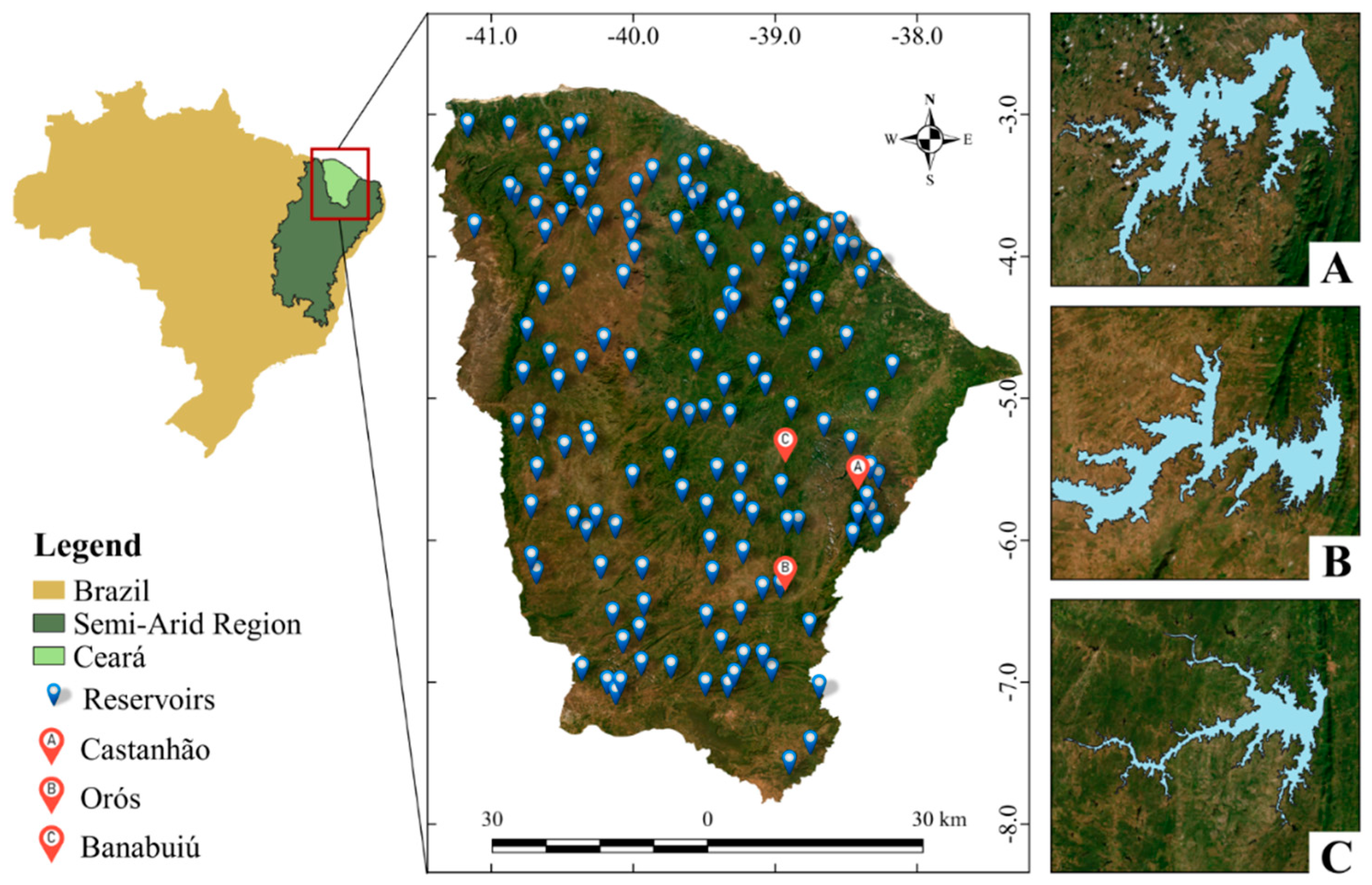
Figure 2.
Correlation matrix for the satellite spectral bands and the Chla.
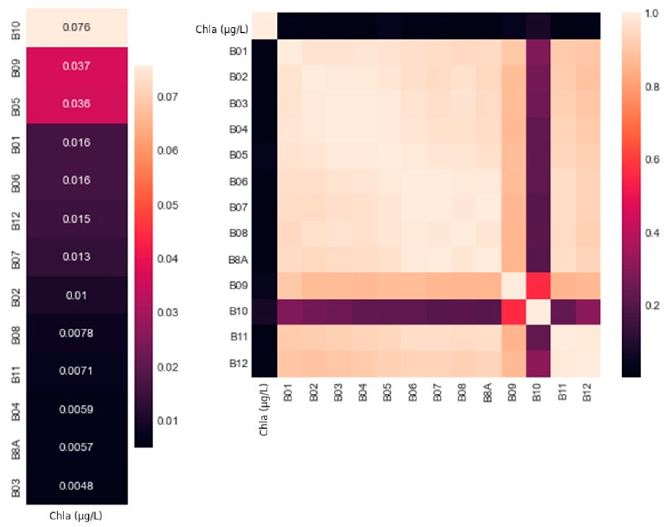
Figure 3.
Correlation matrix for the satellite indexes and the Chla.
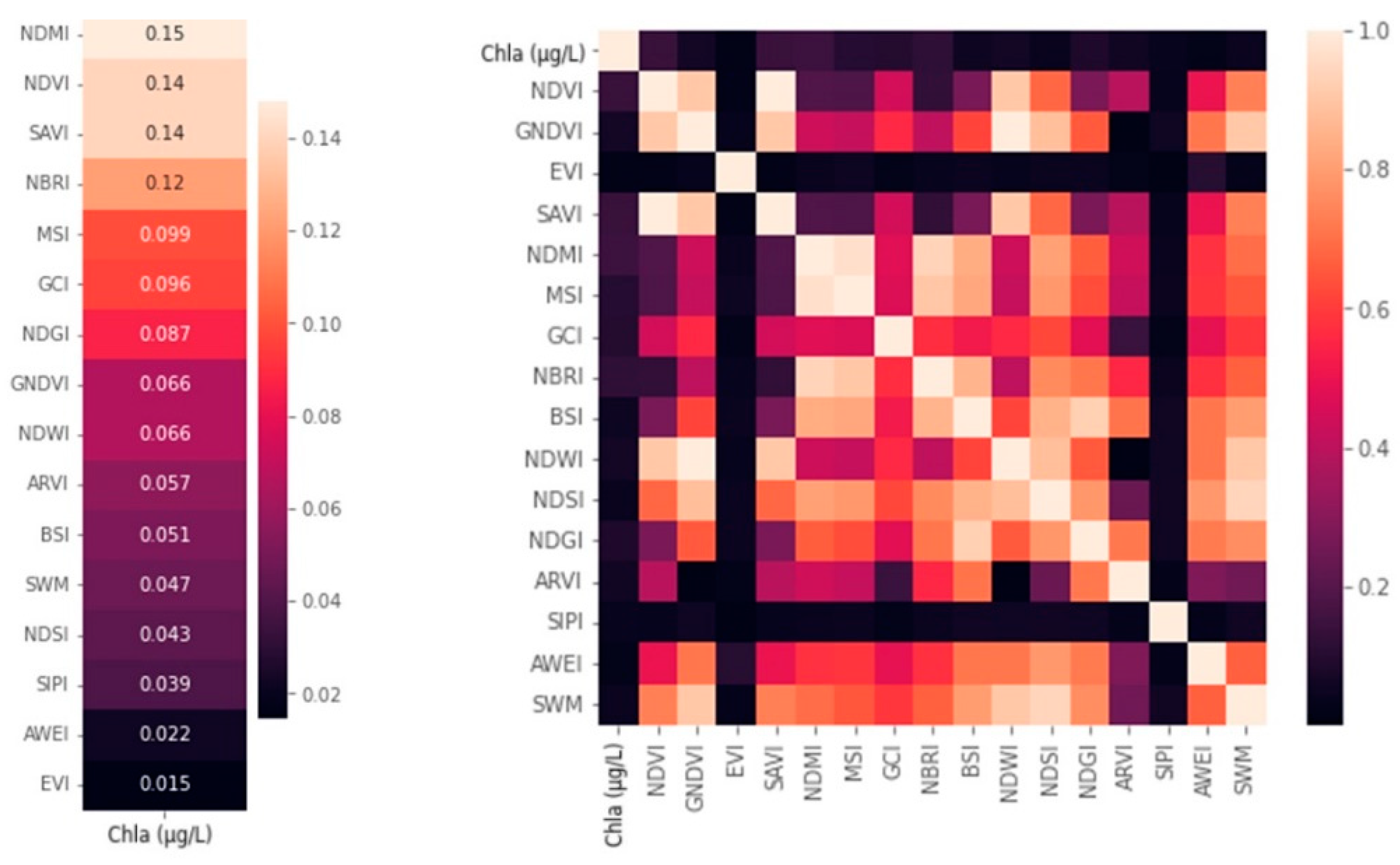
Figure 4.
Selected spectral bands combination. The darker color indicates the best result in terms of R2.
Figure 4.
Selected spectral bands combination. The darker color indicates the best result in terms of R2.
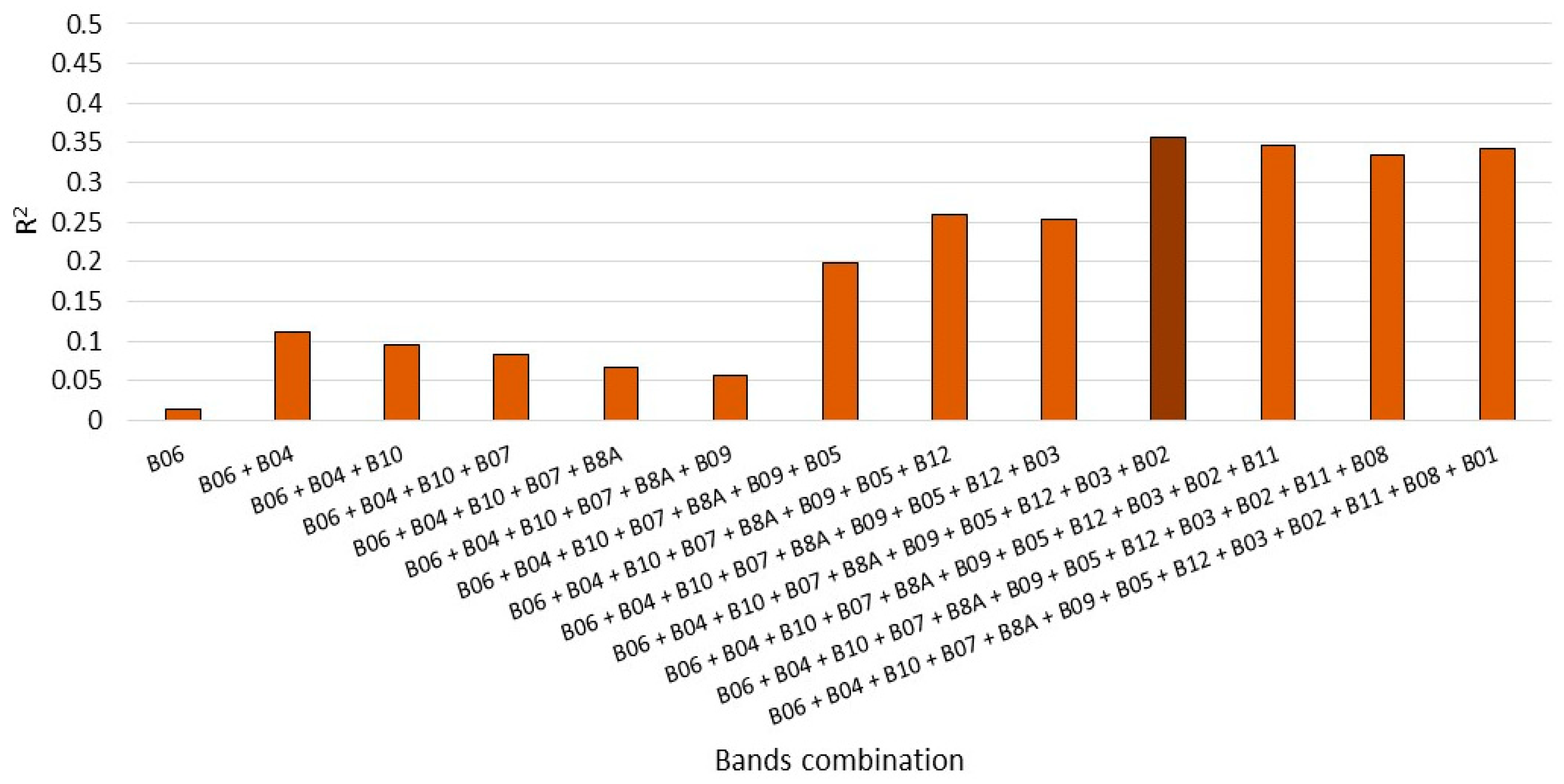
Figure 5.
Selected bands plus the selected spectral indexes combination. The darker color indicates the best result in terms of R2.
Figure 5.
Selected bands plus the selected spectral indexes combination. The darker color indicates the best result in terms of R2.
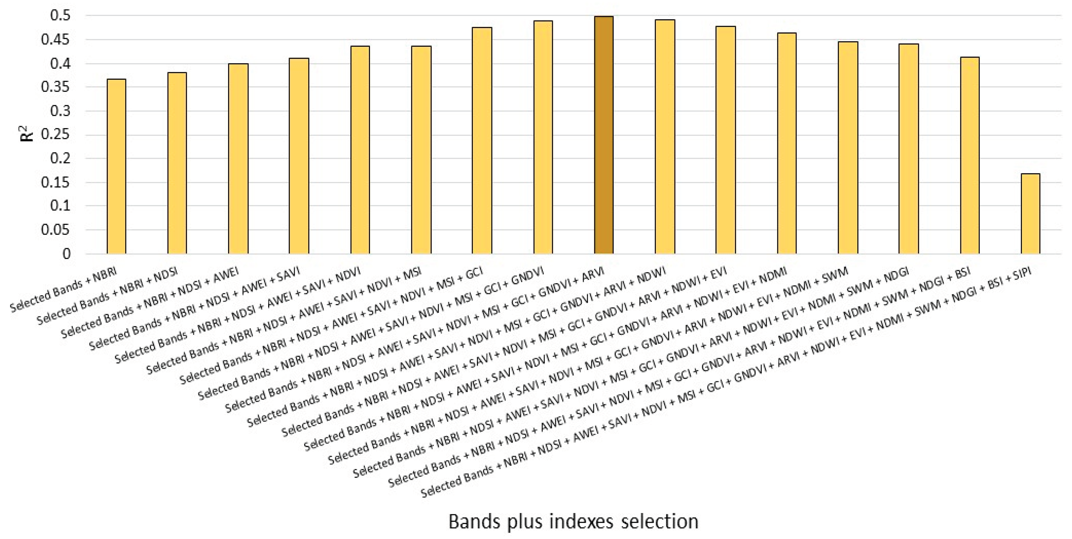
Figure 6.
Boxplots presenting basic statistics of Chla concentrations in logarithmic scale: (A) grouped by sampling year and categorized by season (Rainy: January from April, Dry: remaining months); (B) grouped by the state’s largest reservoirs (Castanhão, Banabuiú and Orós) and all studied reservoirs. The lower and upper limits represent minimum and maximum values. The bottom and top of the box represent the first and third quartiles. Inner lines, asterisks, and circles indicate media, means, and outliers.
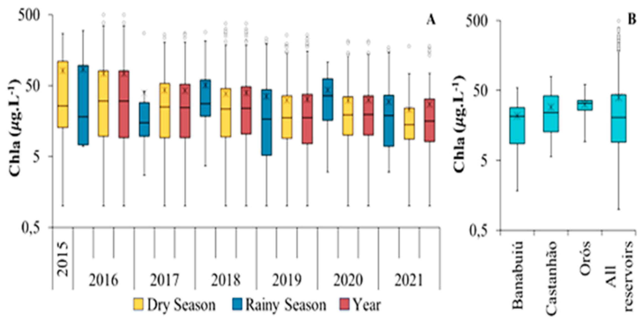
Figure 7.
Scatter plot with marginal distribution for the Chla forecasting by the GMDH model.
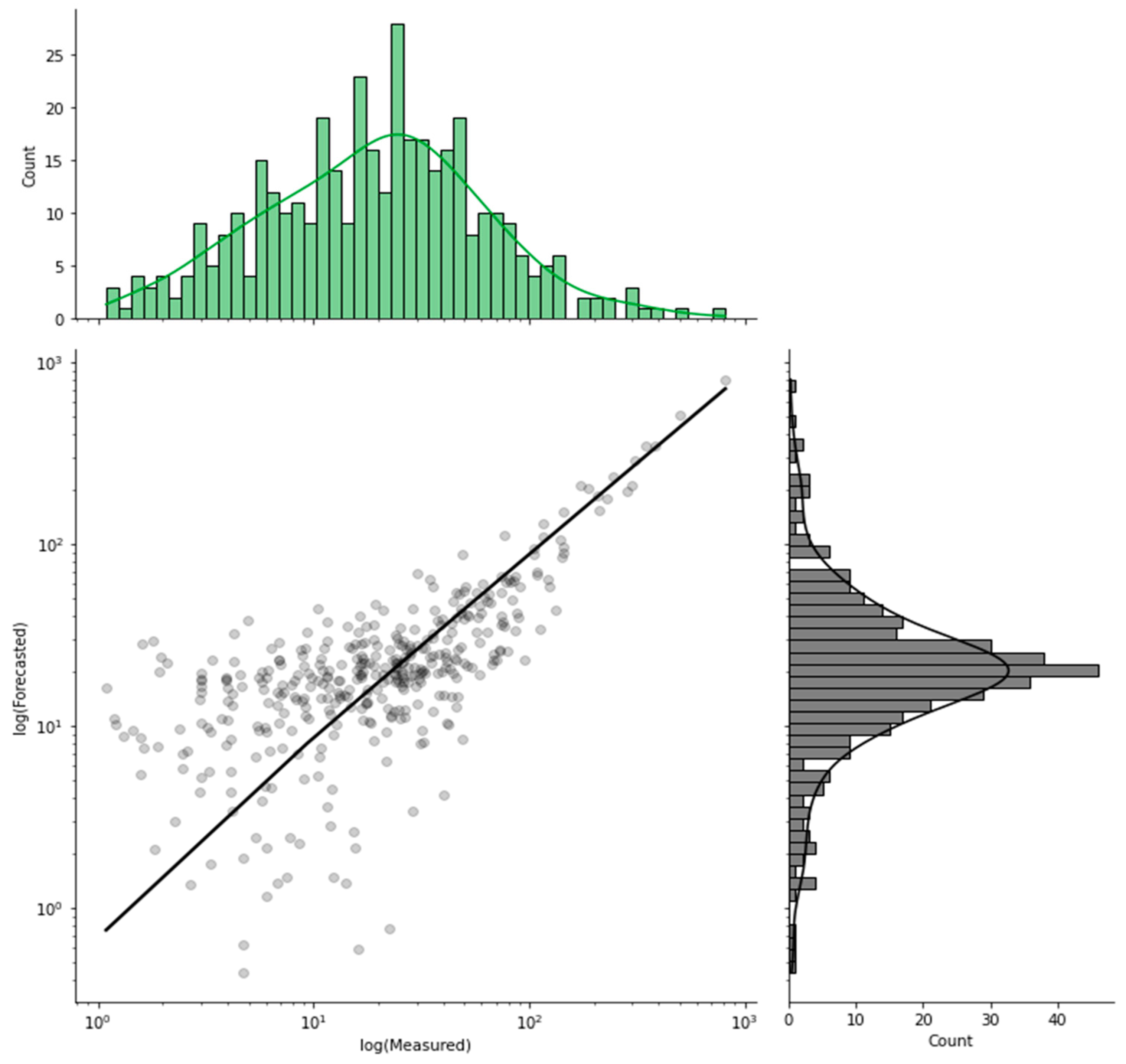

| Band | Central wavelength (nm) |
Band width (nm) |
Spatial resolution (m) |
Band spectral range |
|---|---|---|---|---|
| 1 | 443 | 20 | 60 | Coastal aerosol |
| 2 | 490 | 65 | 10 | Blue |
| 3 | 560 | 35 | 10 | Green |
| 4 | 665 | 30 | 10 | Red |
| 5 | 705 | 15 | 20 | Vegetation red edge 1 |
| 6 | 740 | 15 | 20 | Vegetation red edge 2 |
| 7 | 783 | 20 | 20 | Vegetation red edge 3 |
| 8 | 842 | 115 | 10 | NIR |
| 8A | 865 | 20 | 20 | Narrow NIR |
| 9 | 945 | 20 | 60 | Water vapor |
| 10 | 1380 | 30 | 60 | SWIR-Cirrus |
| 11 | 1610 | 90 | 20 | SWIR 1 |
| 12 | 2190 | 180 | 20 | SWIR 2 |
Table 2.
Results for Chla estimation for the standalone models.
| Model | RMSE (μg/L) |
nRMSE (%) |
MAE (μg/L) |
MAPE (%) |
MBE (μg/L) |
R² | Yeo-Johnson Transformation |
|---|---|---|---|---|---|---|---|
| k-NN | 61.82 | 146.07 | 30.90 | 260.60 | -4.91 | 0.38 | Yes |
| XGBoost | 55.60 | 131.36 | 29.41 | 288.34 | -2.53 | 0.50 | No |
| RF | 56.75 | 134.10 | 29.92 | 311.58 | -1.54 | 0.48 | No |
| SVR | 50.64 | 119.64 | 25.07 | 182.60 | -6.97 | 0.58 | Yes |
| LASSO | 89.87 | 212.34 | 47.41 | 466.35 | -3.60 | 0.41 | Yes |
| GMDH | 20.38 | 53.20 | 14.09 | 102.34 | -4.86 | 0.91 | Yes |
Table 4.
Results for the GMDH model estimation of Chla.
| Model | RMSE (μg/L) |
MAE (μg/L) |
MBE (μg/L) |
MAPE (%) |
R² |
|---|---|---|---|---|---|
| GMDH | 20.38 | 14.09 | -4.86 | 102.34 | 0.91 |
Table 5.
Compilation of results for Chla modeling found in the literature.
| Model | Location | Dataset | RMSE μg/L | R2 | Reference |
|---|---|---|---|---|---|
| Multimodal Deep Learning | Lake Simcoe, Canada | Sentinel-2 and Landsat-8 imagery | 60 | 0.92 | [154] |
| Convolutional Neural Network | Lake Balik, Turkey | Sentinel-2 imagery | 2.9 | 0.95 | [155] |
| Convolutional Neural Network | 11 Lakes in Karlsruhe, Germany | Simulated Chla data used for training, data from SpecWa used for evaluation | 12.4 | 0.82 | [156] |
| SVR | 45 Lakes across China | Sentinel-2 imagery | 6.3 | 0.88 | [157] |
| SVR | Buffalo Pound Lake, Canada | Sentinel-2 imagery | 13.9 | 0.66 | [158] |
| Toming’s index | A Baxe reservoir, Spain | Sentinel-2 imagery | - | 0.86 | [152] |
| 3BSI index | 5 Reservoirs in Ceará, Brazil | Sentinel-2 imagery | - | 0.80 | [13] |
| C2RCC Atmospheric Correction | 6 Reservoirs in São Paulo, Brazil | Sentinel-2 imagery | 2.3 | 0.75 | [159] |
Disclaimer/Publisher’s Note: The statements, opinions and data contained in all publications are solely those of the individual author(s) and contributor(s) and not of MDPI and/or the editor(s). MDPI and/or the editor(s) disclaim responsibility for any injury to people or property resulting from any ideas, methods, instructions or products referred to in the content. |
© 2024 by the authors. Licensee MDPI, Basel, Switzerland. This article is an open access article distributed under the terms and conditions of the Creative Commons Attribution (CC BY) license (http://creativecommons.org/licenses/by/4.0/).
Copyright: This open access article is published under a Creative Commons CC BY 4.0 license, which permit the free download, distribution, and reuse, provided that the author and preprint are cited in any reuse.


