Submitted:
22 December 2023
Posted:
26 December 2023
You are already at the latest version
Abstract
One of the frequently used classes of the sparse reconstruction algorithms is based on the iterative shrinkage/thresholding procedure, where the thresholding parameter controls a trade-off between the algorithm accuracy and the execution time. In order to avoid this trade-off, we propose using a fast intersection of confidence interval method in order to adaptively control the threshold value through the reconstruction algorithm iterations. We have upgraded the two-step iterative shrinkage thresholding algorithm with a such procedure, improving its performance. The proposed algorithm, denoted as the FICI-TwIST, along with a few selected state-of-the-art sparse reconstruction algorithms have been tested on the classical problem of image recovery by emphasizing the image sparsity in the discrete cosine and the discrete wavelet domain. Furthermore, we have derived a single wavelet transformation matrix which avoids wrapping effects achieving significantly faster execution times when compared to more traditional function based transformation. The obtained results indicate competitive performance of the proposed algorithm, even in cases where all algorithm parameters have been individually fine-tuned for best performances.
Keywords:
Compressive sensing
; Fast intersection of confidence intervals
; Image reconstruction
; Iterative soft thresholding
; Signal sparsity
; Sparse reconstruction algorithm.
1. Introduction
The signal sparsity is a signal property which has been used for many decades, mostly for the lossy multimedia compression [1]. The signal is considered K-sparse when most of its energy is located in only K samples, while most of the signal samples are close to zero. In most cases, signals do not exhibit sparsity in the observation domain (e.g. temporal or spatial), however they are sparse in some alternative domain, enabling the lossy compression by discarding the low energy samples. The discrete cosine transform (DCT) and the discrete wavelet transform (DWT) are examples of the sparsity inducing transformations widely used in the popular file formats such as JPEG, JPEG2000, MP3, etc.
The compressive sensing (CS) is a new developing paradigm, which gained interest of many researchers in the last decade, especially after the ground-breaking papers [2,3]. It also exploits the signal sparsity, but in a slightly different way. Instead of recording a full data-set, only a small subset of the original data is recorded, while the missing samples are calculated in a way which will produce the sparsest representation in the a priori known sparse domain. In the real-life situations, the partial unavailability of samples can happen due to the various physical constraints or corrupted data, resulting in the wide-spread application of the CS based methods in the multimedia [1,4,5,6,7], medicine [8,9], geoscience [10,11], radar [12,13], wireless communication [14,15], etc.
In this paper we continue our previous research [6,7] in which we have augmented the two-step iterative shrinkage thresholding (TwIST) algorithm [4] with the fast intersection of confidence interval (FICI) method [16], providing a data-driven threshold value for the TwIST algorithm. This modification has resulted in the sparse reconstruction algorithm, denoted as the FICI-TwIST, in which we have remove the dependency on the user defined threshold value which controls a trade-off between the solution accuracy and the convergence rate of a considered class of the reconstruction algorithms. In this paper we have derived a single wrapped Cohen-Daubechies-Feauveau 9/7 (CDF97) matrix which enabled us to test the previously proposed algorithm not only by emphasizing the sparsity in the DCT domain, but also in the DWT domain. Using such matrix, which to the best knowledge of the authors could not be found in the literature, significantly decreased the algorithm execution times, as shown in this paper.
The rest of the paper is organized as follows. Section 2 gives a theoretical background behind the sparse image reconstruction, derives the used transformation matrices, and introduces the proposed reconstruction algorithm, while Section 3 presents the simulation results. Section 4 gives the concluding remarks.
2. Sparse Image Reconstruction
2.1. Problem Formulation
Let denote a grey-scale image with pixels, and let denote an invertible linear transformation, such that:
resulting in being K-sparse, where . For more convenient mathematical notation, we will rewrite (1), where both and are column vectors:
where is the transformation matrix performing equivalent transformation as in (1). Section 2.3 provides more detailed discussion about the used transformation matrices , their 1D equivalents , and their inverses.
Let denote a column vector of available image pixels randomly selected from , where is the measurement matrix, where each row contains a single entry with the value of 1 (the rest being zeroes), connecting a available pixel with a image pixel. By combining with (2) we define the sparse reconstruction problem:
where is the truncated backward transformation matrix with deleted rows corresponding to the missing samples. In the similar way, matrix , used in future expressions, represents the expanded forward transformation, where the missing samples are set to zero prior to the forward transformation. Since matrix is not invertible, the following unconstrained optimization problem has to be solved [4,5]:
where is the regularization function, while is the regularization parameter. The first term can be interpreted as the error measuring function weighted by the 1/2, while the second term, weighted by , measures the signal property which we want to attain through the optimization procedure. Because of this, can be interpreted as a parameter which controls the solution accuracy: for larger values, the second term becomes more important in the minimization, that is, the first term (i.e. reconstruction error) becomes less important [4,5].
2.2. Problem solution with the -norm minimization
The regularization function plays the most significant role in the previously described optimization problems, as it is a function to be minimized. As already stated, its role is to emphasize the a priori known solution property which in this case is the signal sparsity. In other words, minimizing should maximize the number of zero valued samples in . The best function for this task is the -norm, as it counts the number of non-zero samples. However, the downside of the -norm minimization is that it is a NP-hard combinatorial problem, usually solved with the greedy algorithms, by searching for a good local minima, instead of the global one [17]. Because of this, this problem is often relaxed with the easier to solve convex problem of the -norm minimization [4,5,17,18], hence introducing a new problem: the objective function does not measure an exact signal property which we want to attain. A more detailed survey of the sparse reconstruction algorithms is given in [1,19,20].
By using the -norm based regularization function, we can rewrite (4) as:
allowing a small difference, , between the available pixels and their reconstructed counterparts in order to account for noise. This expression can be further simplified by using the Moreau proximity operator [21]:
Note that the soft-thresholding parameter is the regularization parameter from (4), and in a content of (6) can be interpreted in a similar fashion: a parameter which controls a trade-off between the solution accuracy and the convergence rate. With a higher value, the input signal is going to be thresholded more strictly, resulting in a lower accuracy and a faster convergence rate, and vice versa [4,5].
An example of the sparse reconstruction algorithm which achieves the -norm minimization through iterative soft-thresholding is the TwIST algorithm [4]:
where and are the user defined TwIST relaxation parameters controlling the averaging weights between the current and the previous two solutions. The final solution is obtained by iterating (7) until the stopping criterion is satisfied. In this paper we have used two stopping criteria: (1) the relative change of -norm between the solution of two consecutive algorithm iterations drops bellow , or (2) the maximum number of iterations, , has been reached.
2.3. DCT and DWT Transformation Matrices
The DCT matrix is given by:
for . The transformation matrix, , used in (2), is then simply defined through the Kronecker product as:
Note that is real and orthonormal for the DCT, thus inverse calculation is not needed since . The follows the same property, thus , and most importantly .
Unlike the DCT, the DWT matrix is more complex to construct, hence it is usually represented with the filter banks; the analysis bank performs forward, while the synthesis bank backward transformation. In the analysis bank, the approximation vector in the 1st scale is created by filtering the input vector with a low-pass filter, while the detail vector by filtering with a high-pass filter, followed by the down-sampling with a factor of two. In this fashion, all subsequent scales perform filtering and down-sampling of the approximation vector from the previous scale, ultimately resulting in the scale approximation vector and the 1st - scale detail vectors. In the synthesis bank, the approximation and detail vector of the scale are up-sampled by a factor of two, respectively filtered with a low-pass and a high-pass filter, and summed, creating the approximation vector of the scale. When the input signal is 2D, both filters are applied both row- and column-wise, decomposing it into the approximation and three detail matrices (vertical, horizontal and diagonal) with every subsequential scale further decomposing only the approximation matrix.
In order to construct the CDF97 matrix of the scale, lets start with the pair of biorthogonal low-pass filters of length and , with the following coefficients, already pre-scaled by a factor of and , respectively [22]:
By using the filter coefficients, we can construct a low-pass portion of the transformation matrix on the scale:
for , , and where , , while the conditions - are listed in the first row of Table 1. Such definition of the wavelet matrix negates the wrapping effects, caused by the filter coefficients wrapping around the matrix edges, avoiding the need for input signal periodization. The first condition sums the coefficients in the last columns of the first rows with the appropriate coefficients in the first columns. In the similar way, the second condition sums the coefficients in the first columns of the last rows with the appropriate coefficients in the last columns. These two conditions, involving indexes and , are only valid for a handful of elements, mainly in the top left and the bottom right corner, while most of the coefficients are calculated just as .
Note, however, such matrix definition restricts the DWT scale in two ways: (1) and have to be divisible by , and (2) . The first condition is easily avoided by zero-padding, however the second one seriously limits the DWT scale. Since the DWT domain is more sparse the larger the DWT scale is, it is imperative to avoid this restriction. To better understand (11), the coefficient placement in the matrix row is depicted by Figure 1. The second limiting factor ensures that the depicted coefficient wrapping happens no more than once per row, that is, that no more than two coefficients are summed, since (11) requires such condition. However, using the same logic of turning back when the first or last column is reached, with multiple turns we can place all of the filter coefficients regardless the number of columns, resulting in the matrix entries which are sums of more than two filter coefficients.
In a similar fashion, we can design a high-pass portion of the transformation matrix on the scale. Filter coefficients are calculated as , and matrix is generated analogous to (11), with the conditions - listed in the second row of Table 1. The only difference is caused by the indexing difference between and , since the coefficients are shifted by one.
Matrix performs a single scale transformation from the scale to the scale. In order to create a complete transformation matrix from the 0 to the scale we need to consecutively multiply corresponding matrices, defining the complete matrix representation of the analysis filter bank [23]:
However, due to the image 2D nature, if we apply such matrix to (1), or use the Kronecker product (9) for (2), the result will differ from the traditional DWT definition. Not only the approximation sub-matrix is going to be decomposed in all subsequent DWT scales, but the horizontal and vertical detail sub-matrices as well. Although not ’wrong’, we wanted to maintain the traditional DWT definition, thus is calculated by applying the Kronecker product for each sub-matrix block separately [23]:
As in the DCT case, we again want to avoid the inverse calculation of the relatively large matrix . However, the DWT matrix is not orthonormal, thus , , and most importantly , and this is where the biorthogonal property helps. Although quite possible, we will not calculate the inverse in a traditional way, but rather construct a matrix , using the same coefficients (10), with a similar procedure. The low-pass filter matrix, , is constructed from the coefficients , while the high-pass filter matrix, , is constructed from the coefficients . Both matrices are generated analogous to (11), while the conditions - are listed in the last two rows of Table 1. While most of the coefficients are calculated in the same way (as ), the wrapping effects in the synthesis filter bank are dealt column-wise, resulting in a slight condition differences. The matrix , representing the entire synthesis filter bank, is then constructed analogous to (13).
It is also worth mentioning that (11) is only valid for all four matrices if the filter coefficients are symmetric; in the backward mode we did not take into account mirroring in the wrapping effects. Such compromise has been taken in order to provide elegancy of a single expression valid for all four matrices. In more general terms, both and should be multiplied with in the backward mode, while in both indexes have an additional shift after the multiplication.
2.4. FICI based adaptive thresholding
As already stated, the performance of the sparse reconstruction algorithms which achieve minimization through soft-thresholding is highly dependent on the regularization parameter in (4), that is, the threshold value in (6), controlling a trade-off between the solution accuracy and the convergence rate. In order to achieve both benefits, can be variable through the algorithm iterations: starting relatively high and decreased as the algorithm is converging towards the optimal solution. In our previous research [6,7], we have proposed the FICI-TwIST algorithm, providing an adaptive threshold value calculation in every TwIST iteration. The FICI method searches the vicinity of the specific signal sample for a region with statistically similar amplitude values, which we have used in order to find a region with the statistically lowest amplitudes to be thresholded. The complete FICI-TwIST pseudo-code is given in Algorithm 1, while more detailed discussion can be found in [6,7].
| Algorithm 1 The FICI-TwIST algorithm. |
Ensure: , , , , , , , ,
|
3. Results and Discussion
The reconstruction performance of the proposed algorithm has been tested on a standard grey-scale test image lenna, pre-scaled to pixels for both the DCT and the DWT as the sparsity inducing transformations in two scenarios: (1) the image has been divided into blocks with each block processed individually; (2) without the block division. The DWT scale was set to its maximum: (1) and (2) in order to produce the sparsest domain. In the first scenario the transformations have been implemented exactly as described in Section 2.3, while the second scenario implements the DWT with lifting scheme, while the DCT using MATLAB build-in function, since the transformation matrix would require 16GB of memory space using a single precision float.
The reconstruction performance has been evaluated in terms of the mean square error (MSE) and the algorithm execution time, while the FICI-TwIST algorithm has been compared with the following state-of-the-art reconstruction algorithms: the TwIST [4], the Split augmented Lagrangian shrinkage algorithm (SALSA) [5], the Nesterov algorithm (NESTA) [18], and the your augmented Lagrangian algorithm for (YALL1) [17]. The simulations have been performed for a range of CS ratios, , while the stopping criteria have been set to and . For each CS ratio, the results have been averaged over runs with the randomly generated measuring matrices. All algorithm parameters have been fine-tuned for best performance with the CS ratio of 0.4, which in the hindsight, did not highlighted the main advantage of the proposed algorithm: its adaptivity; however, ’sabotaging’ other algorithms would be, lightly said, dishonest.
The obtained MSE values are presented in Figure 2, while the algorithm execution times are presented in Figure 3. When image is divided into blocks, SALSA (for the DCT) and TwIST (for the DWT) run significantly worst than the other algorithms for lower CS ratios, however, in general all algorithms have very similar reconstruction performances, likely due to the mentioned parameter fine-tuning. In the block scenarios, the FICI-TwIST runs very similar to the NESTA, almost completely overlapping over the entire CS range, together being the most successful algorithms: in the DCT case the FICI-TwIST is slightly worst, while in the DWT case slightly better. When image is not divided into blocks, the FICI-TwIST, in general, is the second best for the lower CS ratios, and worst for the higher CS ratios. In both scenarios, our simulations have shown that the DCT outperforms the DWT in MSE terms. This is specially noticeable in the block scenario where a possible explanation is that the selected block size results in the less-sparse transformation due to the DWT scale limit.
The algorithm execution times are, in general, constant over the entire CS range, having relatively similar ratios between the algorithms in all four scenarios. The FICI-TwIST runs slowest, while the TwiST algorithm runs fastest. This was to be expected, since FICI-TwIST requires constant re-calculation of the mean value and the standard deviation over the increasing window length, while TwIST is the relatively simple algorithm. This fact could be alleviated by skipping the threshold calculation in some of the FICI-TwIST iterations. In the block scenarios, there is very little difference in the algorithm execution times between the DCT and DWT, which was expected, since both transformations involve matrix multiplication. In addition, the block scenario is, in general, two times faster, regardless the algorithm and the sparsity inducing domain. Due to our simulation setup, it is hard to distinguish between the impacts of different implementations vs block size on this fact; however using the function based transformation in block scenario increased the execution times by a factor of and , for the respective algorithm and domain. It is also mention worthy a FICI-TwIST strange behavior: in the DCT case there is very little difference in the execution times between the block and non-block scenario, resulting in the second best execution time for the non-block scenario. On the other hand, in the non-block DWT scenario, execution time started to increase in the middle CS ratios.
In our simulations, the CS ratio of 0.4 have shown to be borderline, with lower ratio resulting in the visually significantly worse reconstruction performance, while on the other hand a higher CS ratio results in a visually undistinguishable images. This fact guided us to fine-tune parameters for this specific ratio, and this is why we have shown the algorithm convergence rate (in terms of MSE) and cumulative execution times over algorithm iterations in Figure 4 and Figure 5, respectively. Figure 5 reveals that all iterations within a specific algorithm take relatively similar time; with an exception of the proposed algorithm in the DWT block scenario. In all cases, the MSE value settles between the 150th and 200th iteration; however only TwIST and NESTA did not exit due to the iteration limit, with all other algorithms running full iterations. This reveals a shortcoming of the selected exit criterium (the relative -norm change), and reveals a possibility for decreasing the execution times by selecting some other, more appropriate criterium. However, in a real-life implementation, not having access to the original image, limits the design space for such criterium. Also to note, the proposed algorithm in the block scenarios experiences the second best convergence rate in the starting iterations, with only YALL1 having better MSE improvement per iteration.
A single, randomly selected run with the CS ratio of 0.4 is shown in Figure 6, Figure 7, Figure 8 and Figure 9 for all four cases. By visual inspection, we can confirm that all scenarios run very competitive, with blocked DWT being an outlier due to already mentioned DWT scale limit. In this scenario, the TwIST algorithm did not converge for some of the blocks. If we compare Figure 6 and Figure 9, in authors opinion two best visually performing cases, Figure 6 (blocked DCT) seems to be a little more sharper, revealing more of the reconstruction defects, while Figure 9 (whole DWT) is much smoother, and (perhaps) visually better looking. However, we leave a task of subjective image quality assessment to a reader, since such task is hard, if not impossible to numerically evaluate.
We have also performed simulations on two more standard test images: barbara and cameraman with a same simulation setup. The obtained results are not significantly different to the previously discussed results for lenna, thus we have shown only the MSE values throughout different CS ratios in Figure 10 and Figure 11.
4. Conclusion
In this paper we have demonstrated the effectiveness of the sparsity based image recovery: in our test scenarios images with up to 60% of missing pixels have been successfully recovered. More importantly, we have derived a matrix-based wavelet transformation which is based on the CDF97 wavelet, achieving a significant reduction (by a factor of 10) in the considered sparse reconstruction algorithms execution times when compared to the function-based transformation. This allowed us to expand our previous research in which we have proposed the sparse reconstruction algorithm with its main advantage being its adaptivity by taking the variable iterative thresholding steps. In our simulations, we have shown that even in the scenarios where all individual parameters of the considered state-of-the-art algorithms were fine-tuned, the proposed algorithm runs very competitively, even outperforming them in some specific cases.
Our simulations have also revealed that the DCT domain outperforms the DWT domain by a great margin in the reconstruction process, at least in the MSE terms; however, more detailed simulations with variable block sizes should be performed in order to confirm such conclusion. In addition, the relative -norm change has shown to be inadequate algorithm exit criterion; thus designing a more image specific criteria would further decrease the reconstruction execution times.
Author Contributions
Conceptualization, I.V. and V.S.; methodology, I.V.; software, I.V.; validation, I.V. and V.S.; formal analysis, I.V.; investigation, I.V.; resources, I.V.; data curation, I.V.; writing—original draft preparation, I.V.; writing—review and editing, V.S.; visualization, I.V.; supervision, V.S.; project administration, V.S.; funding acquisition, V.S. All authors have read and agreed to the published version of the manuscript.
Funding
This work has been fully supported by the University of Rijeka under the project number UNIRI-TEHNIC-18-67.
Data Availability Statement
The data presented in this paper is available on request from the corresponding author.
Conflicts of Interest
The authors declare no conflict of interest.
References
- Stanković, S.; Orović, I.; Sejdić, E. Multimedia Signals and Systems; SpringerLink: Bücher, Springer US, 2012. [Google Scholar]
- Donoho, D. Compressed sensing. IEEE Transactions on Information Theory 2006, 52, 1289–1306. [Google Scholar] [CrossRef]
- Candés, E.; Romberg, J.; Tao, T. Robust uncertainty principles: exact signal reconstruction from highly incomplete frequency information. IEEE Transactions on Information Theory 2006, 52, 489–509. [Google Scholar] [CrossRef]
- Bioucas-Dias, J.M.; Figueiredo, M.A.T. A New TwIST: Two-Step Iterative Shrinkage/Thresholding Algorithms for Image Restoration. IEEE Transactions on Image Processing 2007, 16, 2992–3004. [Google Scholar] [CrossRef] [PubMed]
- Afonso, M.V.; Bioucas-Dias, J.M.; Figueiredo, M.A.T. Fast Image Recovery Using Variable Splitting and Constrained Optimization. IEEE Transactions on Image Processing 2010, 19, 2345–2356. [Google Scholar] [CrossRef] [PubMed]
- Volaric, I.; Sucic, V. Sparse Image Reconstruction via Fast ICI Based Adaptive Thresholding. 2022 30th Telecommunications Forum (TELFOR), 2022, pp. 1–4. [CrossRef]
- Volaric, I.; Sucic, V. Adaptive Thresholding for Sparse Image Reconstruction. Telfor Journal 2023, 15, 8–13. [Google Scholar] [CrossRef]
- Da Poian, G.; Bernardini, R.; Rinaldo, R. Separation and Analysis of Fetal-ECG Signals From Compressed Sensed Abdominal ECG Recordings. IEEE Transactions on Biomedical Engineering 2016, 63, 1269–1279. [Google Scholar] [CrossRef] [PubMed]
- Lingala, S.G.; Jacob, M. Blind Compressive Sensing Dynamic MRI. IEEE Transactions on Medical Imaging 2013, 32, 1132–1145. [Google Scholar] [CrossRef] [PubMed]
- Zhou, Y.; Gao, J.; Chen, W.; Frossard, P. Seismic Simultaneous Source Separation via Patchwise Sparse Representation. IEEE Transactions on Geoscience and Remote Sensing 2016, 54, 5271–5284. [Google Scholar] [CrossRef]
- Kumlu, D.; Erer, I. Improved Clutter Removal in GPR by Robust Nonnegative Matrix Factorization. IEEE Geoscience and Remote Sensing Letters 2020, 17, 958–962. [Google Scholar] [CrossRef]
- Stanković, L. ISAR image analysis and recovery with unavailable or heavily corrupted data. IEEE Transactions on Aerospace and Electronic Systems 2015, 51, 2093–2106. [Google Scholar] [CrossRef]
- Akhtar, J.; Olsen, K.E. Formation of Range-Doppler Maps Based on Sparse Reconstruction. IEEE Sensors Journal 2016, 16, 5921–5926. [Google Scholar] [CrossRef]
- Barceló-Lladó, J.E.; Morell, A.; Seco-Granados, G. Amplify-and-Forward Compressed Sensing as an Energy-Efficient Solution in Wireless Sensor Networks. IEEE Sensors Journal 2014, 14, 1710–1719. [Google Scholar] [CrossRef]
- Draganić, A.; Orović, I.; Stanković, S. Blind signals separation in wireless communications based on Compressive Sensing. 2014 22nd Telecommunications Forum Telfor (TELFOR), 2014, pp. 561–564. [CrossRef]
- Volaric, I.; Lerga, J.; Sucic, V. A Fast Signal Denoising Algorithm Based on the LPA-ICI Method for Real-Time Applications. Circuits, Systems, and Signal Processing 2017, 36, 4653–4669. [Google Scholar] [CrossRef]
- Zhang, Y. User’s Guide For YALL1: Your Algorithms for L1 Optimization. Technical report, 2009.
- Becker, S.; Bobin, J.; Candés, E.J. NESTA: A Fast and Accurate First-Order Method for Sparse Recovery. SIAM Journal on Imaging Sciences 2011, 4, 1–39. [Google Scholar] [CrossRef]
- Zhang, Z.; Xu, Y.; Yang, J.; Li, X.; Zhang, D. A Survey of Sparse Representation: Algorithms and Applications. IEEE Access 2015, 3, 490–530. [Google Scholar] [CrossRef]
- Crespo Marques, E.; Maciel, N.; Naviner, L.; Cai, H.; Yang, J. A Review of Sparse Recovery Algorithms. IEEE Access 2019, 7, 1300–1322. [Google Scholar] [CrossRef]
- Combettes, P.L.; Wajs, V.R. Signal Recovery by Proximal Forward-Backward Splitting. Multiscale Modeling & Simulation 2005, 4, 1168–1200. [Google Scholar] [CrossRef]
- Van Fleet, P.J. Discrete Wavelet Transformations: An Elementary Approach with Applications; Wiley, 2019. [CrossRef]
- Wang, H.; Vieira, J. 2-D Wavelet Transforms in the Form of Matrices and Application in Compressed Sensing. 2010 8th World Congress on Intelligent Control and Automation, 2010, pp. 35–39. [CrossRef]
Figure 1.
Placement of the filter coefficients in the matrix row. The first column is skipped based on the conditions listed in Table 1. Only the placement of negative indexes is depicted, however, the same logic applies for positive indexes, which are summed with the existing entries.
Figure 1.
Placement of the filter coefficients in the matrix row. The first column is skipped based on the conditions listed in Table 1. Only the placement of negative indexes is depicted, however, the same logic applies for positive indexes, which are summed with the existing entries.
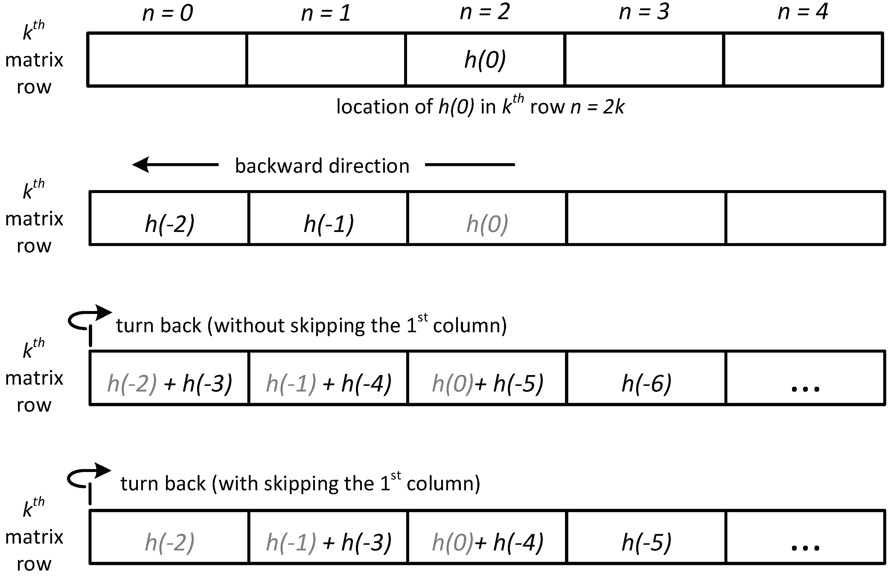
Figure 2.
Average reconstructed MSE values for TwIST (red), SALSA (green), NESTA (blue), YALL1 (magenta), and FICI-TwIST (black) over range; and scenario: (a) DCT blocked, (b) DCT whole, (c) DWT blocked, (d) DWT whole. Range of the zoom inset is .
Figure 2.
Average reconstructed MSE values for TwIST (red), SALSA (green), NESTA (blue), YALL1 (magenta), and FICI-TwIST (black) over range; and scenario: (a) DCT blocked, (b) DCT whole, (c) DWT blocked, (d) DWT whole. Range of the zoom inset is .
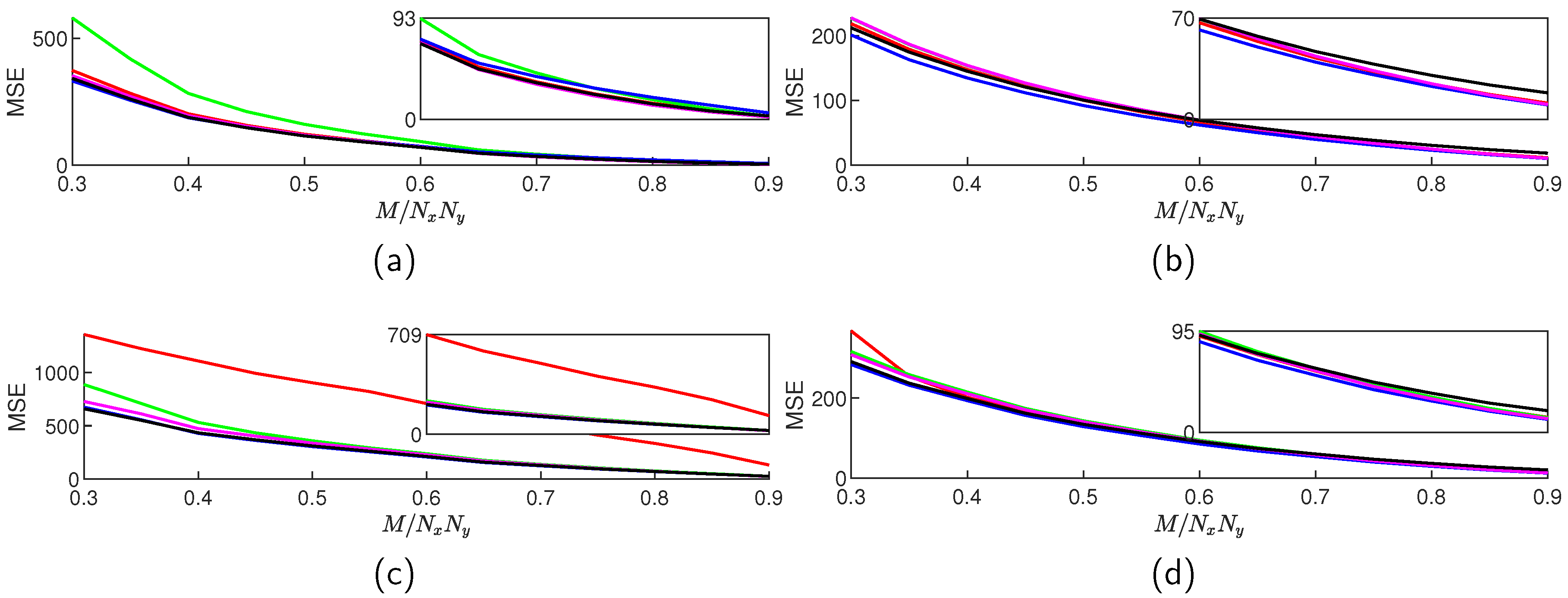
Figure 3.
Average algorithm execution time for TwIST (red), SALSA (green), NESTA (blue), YALL1 (magenta), and FICI-TwIST (black) over range; and scenario: (a) DCT blocked, (b) DCT whole, (c) DWT blocked, (d) DWT whole.
Figure 3.
Average algorithm execution time for TwIST (red), SALSA (green), NESTA (blue), YALL1 (magenta), and FICI-TwIST (black) over range; and scenario: (a) DCT blocked, (b) DCT whole, (c) DWT blocked, (d) DWT whole.
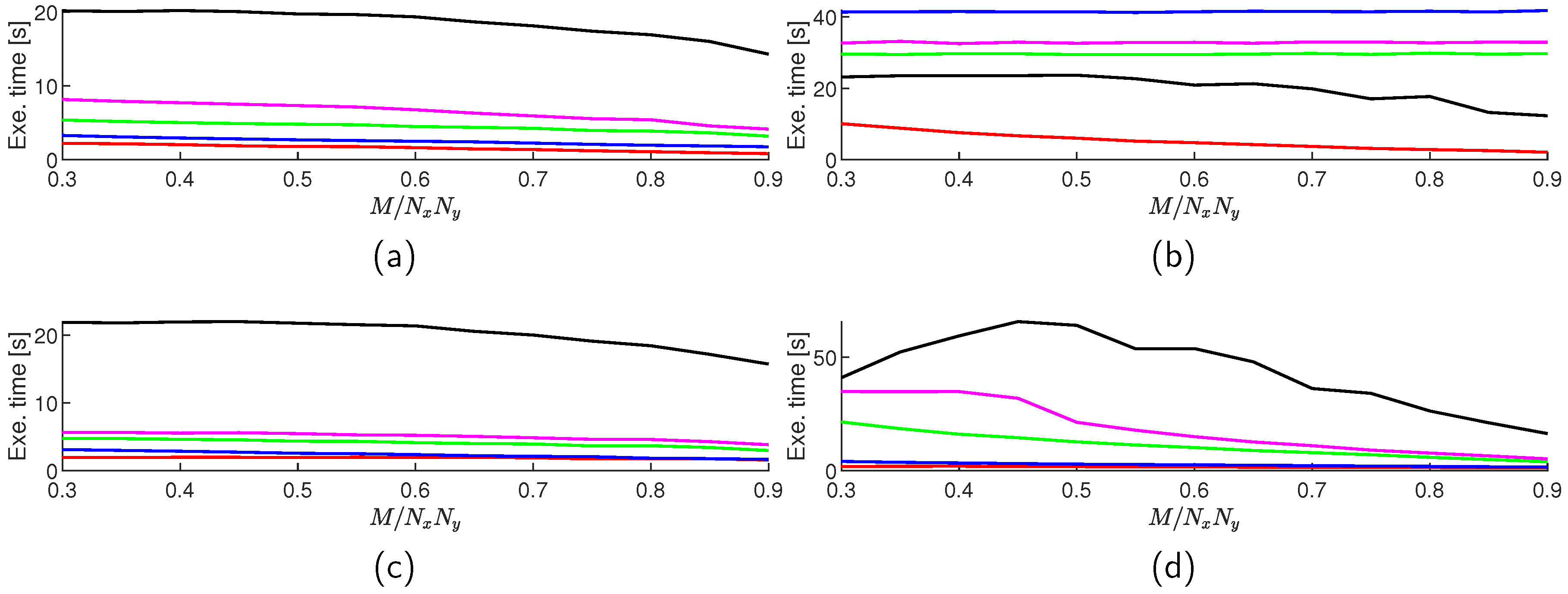
Figure 4.
Average reconstructed MSE values () for TwIST (red), SALSA (green), NESTA (blue), YALL1 (magenta), and FICI-TwIST (black) over algorithm iterations; and scenario: (a) DCT blocked, (b) DCT whole, (c) DWT blocked, (d) DWT whole.
Figure 4.
Average reconstructed MSE values () for TwIST (red), SALSA (green), NESTA (blue), YALL1 (magenta), and FICI-TwIST (black) over algorithm iterations; and scenario: (a) DCT blocked, (b) DCT whole, (c) DWT blocked, (d) DWT whole.
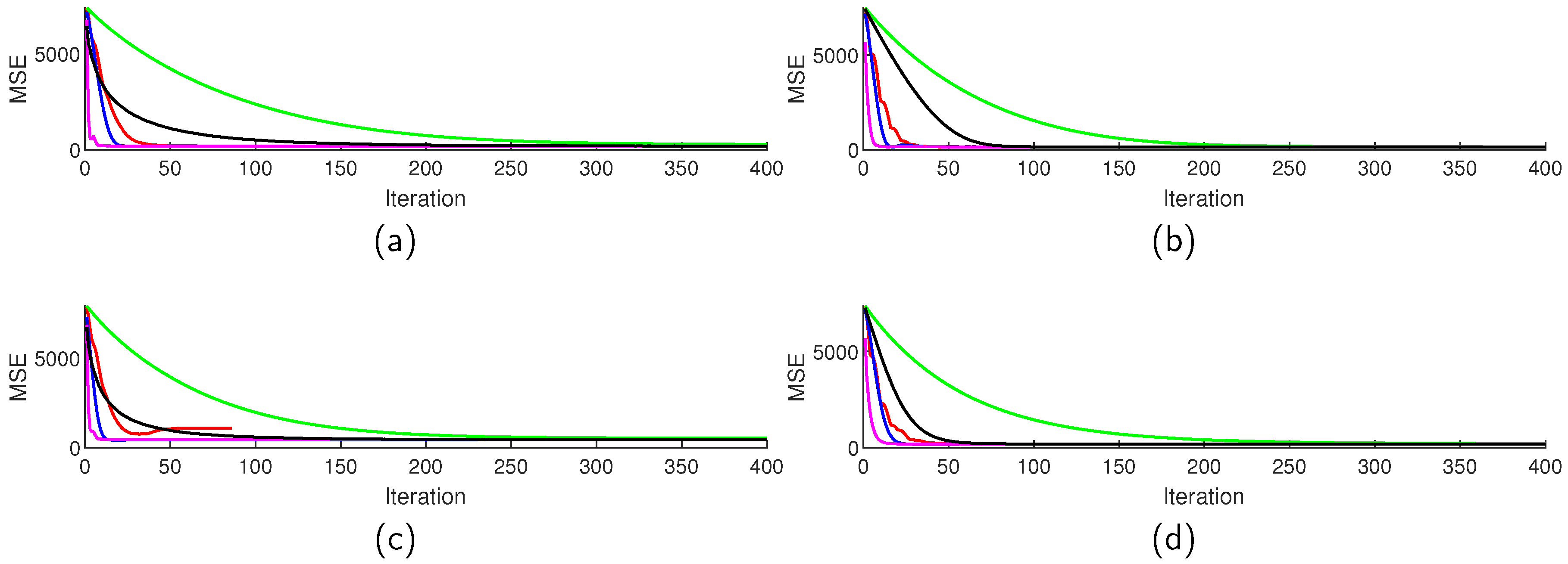
Figure 5.
Average cumulative algorithm execution times () for TwIST (red), SALSA (green), NESTA (blue), YALL1 (magenta), and FICI-TwIST (black) over algorithm iterations; and scenario: (a) DCT blocked, (b) DCT whole, (c) DWT blocked, (d) DWT whole.
Figure 5.
Average cumulative algorithm execution times () for TwIST (red), SALSA (green), NESTA (blue), YALL1 (magenta), and FICI-TwIST (black) over algorithm iterations; and scenario: (a) DCT blocked, (b) DCT whole, (c) DWT blocked, (d) DWT whole.
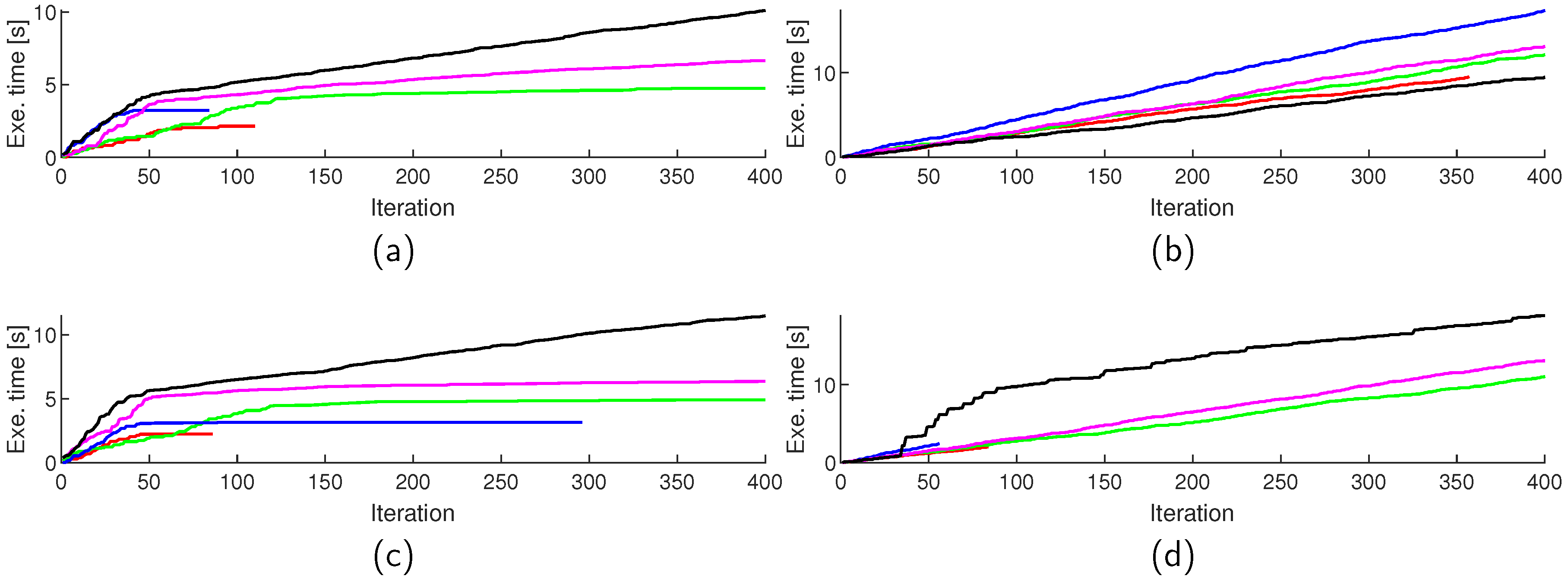
Figure 6.
Sparse reconstruction results for blocked DCT scenario: (a) CSed image (); (b) reconstructed by the TwIST (); (c) reconstructed by the SALSA (); (d) reconstructed by the NESTA (); (e) reconstructed by the YALL1 (); (f) reconstructed by the FICI-TwIST ().
Figure 6.
Sparse reconstruction results for blocked DCT scenario: (a) CSed image (); (b) reconstructed by the TwIST (); (c) reconstructed by the SALSA (); (d) reconstructed by the NESTA (); (e) reconstructed by the YALL1 (); (f) reconstructed by the FICI-TwIST ().
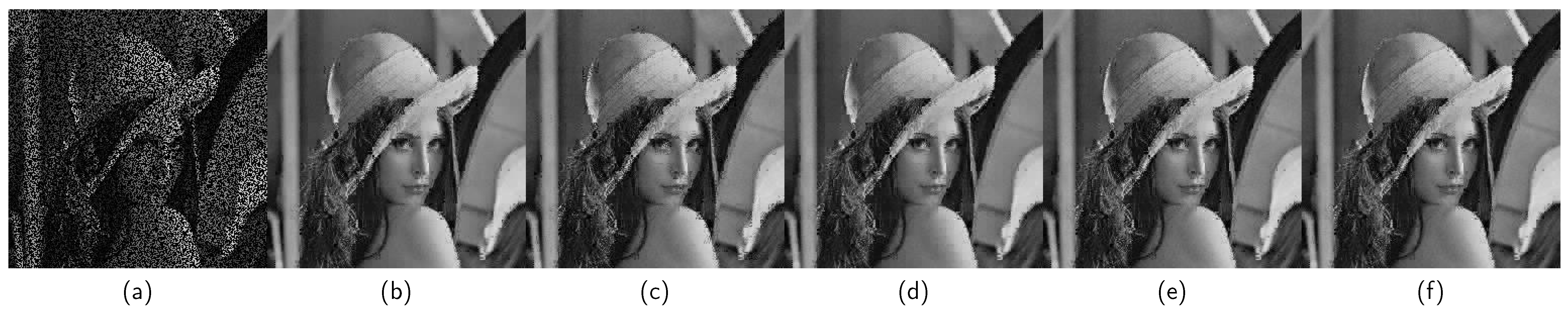
Figure 7.
Sparse reconstruction results for whole DCT scenario: (a) CSed image (); (b) reconstructed by the TwIST (); (c) reconstructed by the SALSA (); (d) reconstructed by the NESTA (); (e) reconstructed by the YALL1 (); (f) reconstructed by the FICI-TwIST ().
Figure 7.
Sparse reconstruction results for whole DCT scenario: (a) CSed image (); (b) reconstructed by the TwIST (); (c) reconstructed by the SALSA (); (d) reconstructed by the NESTA (); (e) reconstructed by the YALL1 (); (f) reconstructed by the FICI-TwIST ().

Figure 8.
Sparse reconstruction results for blocked DWT scenario: (a) CSed image (); (b) reconstructed by the TwIST (); (c) reconstructed by the SALSA (); (d) reconstructed by the NESTA (); (e) reconstructed by the YALL1 (); (f) reconstructed by the FICI-TwIST ().
Figure 8.
Sparse reconstruction results for blocked DWT scenario: (a) CSed image (); (b) reconstructed by the TwIST (); (c) reconstructed by the SALSA (); (d) reconstructed by the NESTA (); (e) reconstructed by the YALL1 (); (f) reconstructed by the FICI-TwIST ().
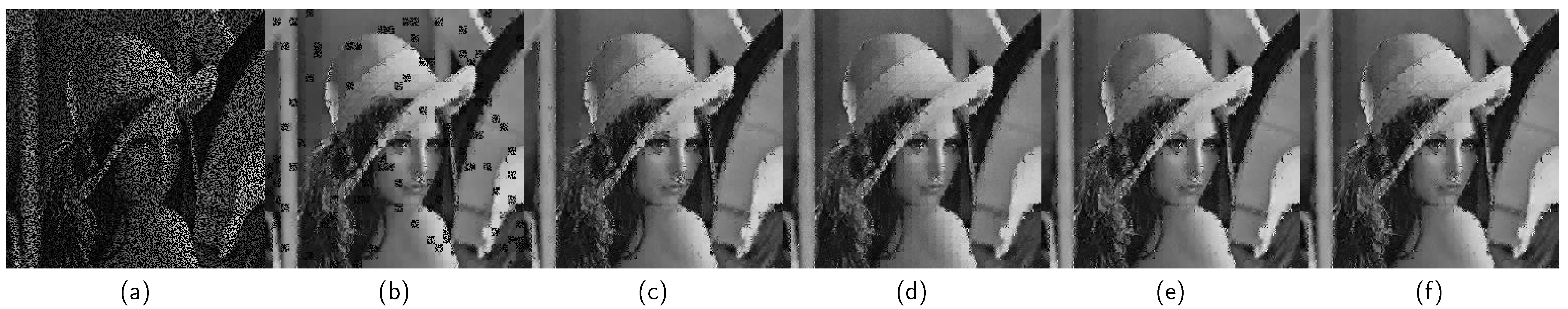
Figure 9.
Sparse reconstruction results for whole DWT scenario: (a) CSed image (); (b) reconstructed by the TwIST (); (c) reconstructed by the SALSA (); (d) reconstructed by the NESTA (); (e) reconstructed by the YALL1 (); (f) reconstructed by the FICI-TwIST ().
Figure 9.
Sparse reconstruction results for whole DWT scenario: (a) CSed image (); (b) reconstructed by the TwIST (); (c) reconstructed by the SALSA (); (d) reconstructed by the NESTA (); (e) reconstructed by the YALL1 (); (f) reconstructed by the FICI-TwIST ().
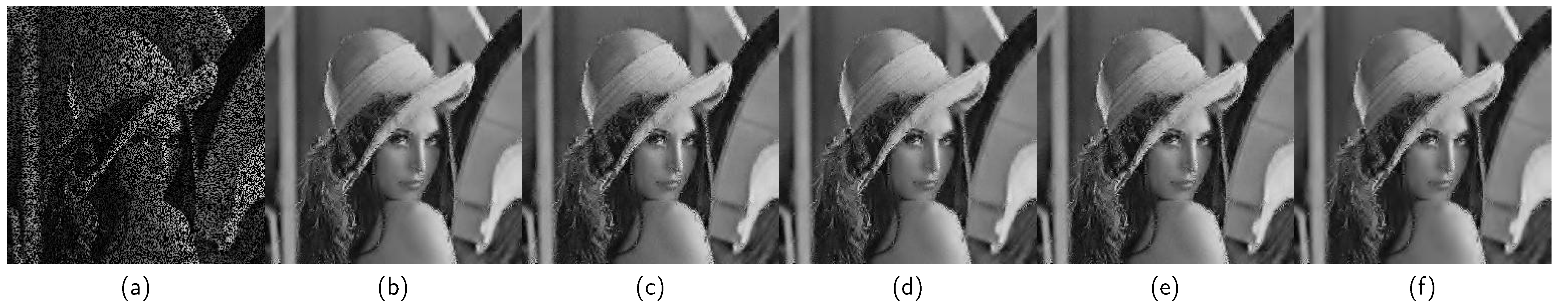
Figure 10.
Average reconstructed barbara MSE values for TwIST (red), SALSA (green), NESTA (blue), YALL1 (magenta), and FICI-TwIST (black) over range; and scenario: (a) DCT blocked, (b) DCT whole, (c) DWT blocked, (d) DWT whole. Range of the zoom inset is .
Figure 10.
Average reconstructed barbara MSE values for TwIST (red), SALSA (green), NESTA (blue), YALL1 (magenta), and FICI-TwIST (black) over range; and scenario: (a) DCT blocked, (b) DCT whole, (c) DWT blocked, (d) DWT whole. Range of the zoom inset is .
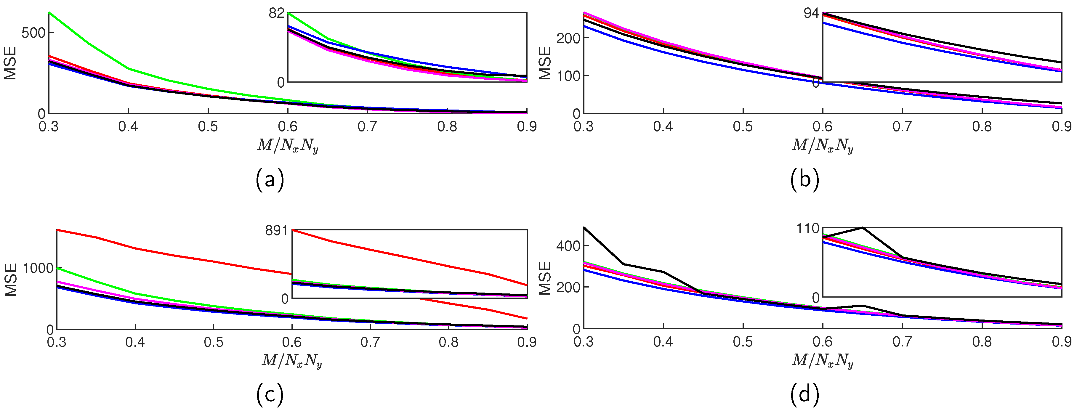
Figure 11.
Average reconstructed cameraman MSE values for TwIST (red), SALSA (green), NESTA (blue), YALL1 (magenta), and FICI-TwIST (black) over range; and scenario: (a) DCT blocked, (b) DCT whole, (c) DWT blocked, (d) DWT whole. Range of the zoom inset is .
Figure 11.
Average reconstructed cameraman MSE values for TwIST (red), SALSA (green), NESTA (blue), YALL1 (magenta), and FICI-TwIST (black) over range; and scenario: (a) DCT blocked, (b) DCT whole, (c) DWT blocked, (d) DWT whole. Range of the zoom inset is .
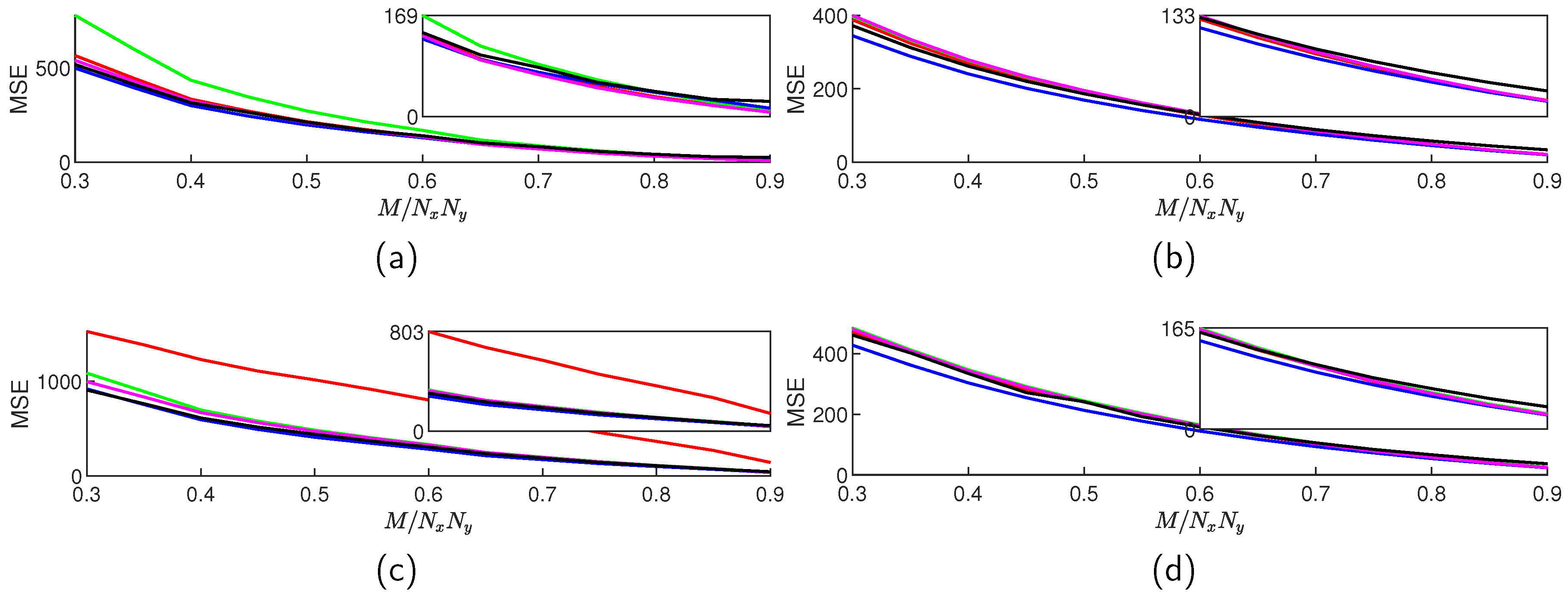

Table 1.
Index restrictions for DWT matrices.
| c1 | c2 | c3 | |
|---|---|---|---|
| and | and | ||
| and | and | ||
| and | |||
| and |
Disclaimer/Publisher’s Note: The statements, opinions and data contained in all publications are solely those of the individual author(s) and contributor(s) and not of MDPI and/or the editor(s). MDPI and/or the editor(s) disclaim responsibility for any injury to people or property resulting from any ideas, methods, instructions or products referred to in the content. |
© 2023 by the authors. Licensee MDPI, Basel, Switzerland. This article is an open access article distributed under the terms and conditions of the Creative Commons Attribution (CC BY) license (http://creativecommons.org/licenses/by/4.0/).
Copyright: This open access article is published under a Creative Commons CC BY 4.0 license, which permit the free download, distribution, and reuse, provided that the author and preprint are cited in any reuse.


