1. Introduction
Foreign object detection is widely used in the industrial field, mainly because industrial products generally have high output value, so people are more willing to invest expensive technologies and devices in this field. However, compared to industrial products, agricultural products have lower value, and these expensive devices are rarely widely used in the agricultural field. Especially, in the early stage in agricultural production, there are foreign objects as metal screw and rubber from ageing machines, and clod rock from farmland, these object will damage the equipment if not be moved timely, due to the complex environment, some precise and active devices are difficult to deploy. Therefore, in agricultural of object detection, there is an urgent need for a detection method that is fast, accurate, low-cost, and convenient for on-line deployment. In recent years, wireless sensing methods based on Radio Frequency have been attracted people’s great attention. It is a widely used technology in the field of the Internet of Things (IoT), smart agriculture and so on, and it is considered as one of the most influential technologies in this century. The RFID based wireless sensing is one the core technologies in many fields, due to its low-cost, labeling, easy deployment, and high sensing accuracy, such as indoor scene sensing and positioning [
1,
2,
3], smart agriculture [
4,
5,
6,
7], humidity detection [
8], trajectory tracking and attitude recognition [
9,
10,
11]. In the application of metal detection and material sensing [
12], especially in localization [
13,
14], RFID technologies have been developed many product devices due to their low-cost and convenient deployment [
15]. More recently, the widespread of these applications in indoor positioning has gradually received great attention from researchers, brought us very meaningful ideas.
The LANDMARC system [
16] used RFID technology to locate objects inside buildings. It is an early RFID based indoor positioning system. However, the RFID tags in this system are customized active tags, which are costly and difficult to deploy. Subsequently, [
17] utilized commercial RFID tags to locate the target, it achieved localization without hardware modification, which can greatly reduce the costs. However, due to the coarse-grained of RSS, the localization accuracy is not satisfied. [
2] proposed a hierarchical classification localization system to accurately locate the target position, which divides the environment into multiple regions to reduce the number of training and prediction classes for the classifier. The system can achieves precise positioning, while its robustness is challenged because it significantly reliance on classifier design and the number of training samples. The authors in [
18,
19,
20] all utilized RFID methods to achieve the localization of moving objects, where [
18] offered a way to identify objects without any contact, it proposed a new and innovative approach for the localization of moving object using a particle filter by incorporating RFID phase and laser-based clustering. [
19] proposed a method based on an RFID tag array and laser ranging information to locate humans movement, which is similar to the method used in our paper, However, it requires the human to be equipped with a tag array limiting its application. [
20] Chen presented an approach to integrate RFID phase and laser range information for the tracking of dynamic objects in an environment, it determined the locations of objects by comparing the velocities estimated from two different systems. These proposed approaches uses the commercial off the shelf RFID devices and does not require the modelling of radio signal propagation, which attempts to overcome the shortcomings of [
2] and uses mathematical models to locate the target. However, the mathematical model failed to be universally applied in various tasks. In addition, although phase can accurately sense the target position, its periodic characteristics limit its application. [
21,
22,
23] all proposed a 3D localization scheme based on RFID tag arrays, where [
22] only used one mobile RFID antenna for target localization, [
21] used the signal arrival angles as features for localization, In addition, and [
23] deployed multiple tags on the upper parts of human limbs, used dual antennas to obtain the tag phase, and used phase changes to track the 3D position of human bones. They have achieved relatively satisfactory accuracy, but the tag need be attached to the target, which limits the practical application.
Inspired by the above, we use multi RFID tags to form tag matrices to achieve sensing, recognition and localizing in NLOS scene. The principle of sensing and localizing foreign objects in medium is that, when RFID tags receive electromagnetic waves from RFID antenna, they will be activated, and emit signals back to space in the form of scattering. When the signal propagates in the medium and encounters foreign objects, they will be changed. The system detects and senses foreign objects using the changing features in the signals when there are objects in medium.
In summary, most RFID based sensing technologies either use coarse-grained RSS [
25,
26,
27] or fine-grained phase [
29,
30,
31] to sense targets. Different from the previous studies, we use the scattering coefficient
combined with the RSS as features for sensing the target, which can compensate for the problem of inaccurate caused by coarse-grained of RSS and can eliminate the localization ambiguity caused by phase periodicity. Moreover, previous studies have mostly focused on attaching tags to targets in Line-Of-Sight (LOS) scenarios to sense their properties, however in many applications (such as in NLOS scenarios), the targets are unknown or invisible, i.e. whether the target exists are unknown, and the positions are also unknown, which is a challenging issue. Based on the above, we propose a recognition and localizing system using non-contact method in NLOS scenarios. There are two steps for sensing in this system, the first steps is to detect whether there are foreign objects in medium (such as wheat and Seedless cotton), the second step is to determine the 3-D positions of objects. We use the vector V(
,RSS) as features and propose Euclidean-distance-ratio (EDR) method to detect if there are foreign objects. A projection method is proposed to determine the position of object. The cost of the system is low, and each tag only costs about 0.3 RMB, making it possible for large-scale application. Moreover, the system can work well in many deployment environment, as long as the RFID antenna can communicate with the tags, the system can sense foreign objects in NLOS with bad and complex environment.
2. Architecture of the sensing system based on tag matrix
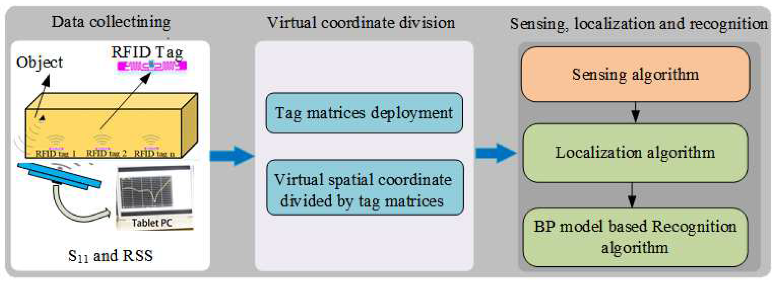
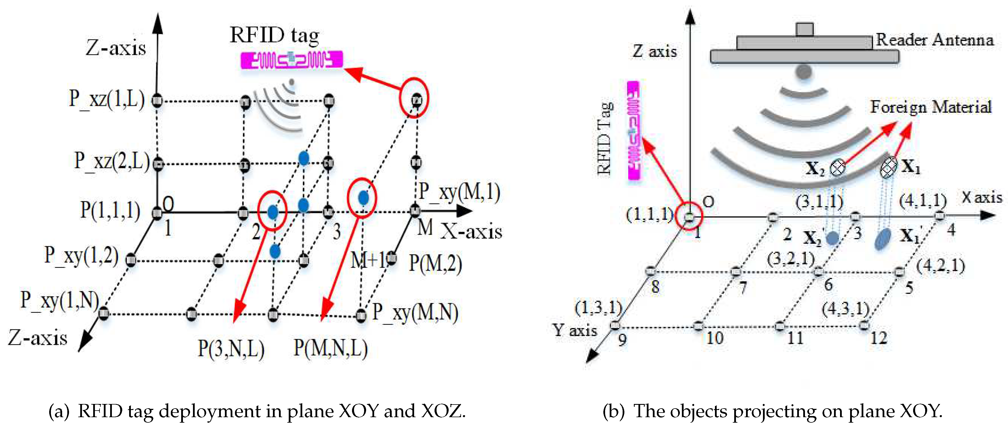
There are four modules in this system, including data collecting, virtual spatial coordinates division, foreign object localization and recognition. In the data collecting module, it uses a wireless and passive sensing method based on RFID, which is easy to deploy with low cost. In virtual spatial coordinates division module, the sensing space is divided into multiple virtual coordinates based on the tags matrices deployed on two different planes, i.e. XOZ plane and XOY plane, as shown in Figure 5, the blue solid points represent the virtual position, black hollow points represent tags matrix points deployed in XOZ plane and the XOY plane respectively. If there is a foreign object, it will be located near these virtual intersections, and the intersection closest to the foreign object is considered as its coordinate. For object sensing module, since the object to be sensed is unknown (the presence or absence of foreign objects is unknown), the system first collects the signal features when there are no foreign objects, the signal features collection is one-time and they are stored in the database for comparison to determine the presence of foreign objects. The system detects a foreign object by comparing the changes of the signal before and after the appearance of the foreign object in the sensing space. In the sensing and localization module, the main purpose of sensing foreign objects is to find and remove them. System determines objects position in the coordinates by virtual coordinates, so that people can remove objects timely. We use a "projection" method to determine the virtual coordinates of foreign objects in the sensing space by deploying tag matrices on two planes (XOZ plane and XOY plane). In the recognition module, we utilized BP network model to recognize the types of the objects using the collected data.
Figure 1 shows the system flowchart of the four modules.
3. Feasibility analysis
This section presents the preliminaries study in sensing and localization object using scattering coefficient () and received signal strength (RSS) in a medium (such as cotton and wheat).
3.1. based sensing model
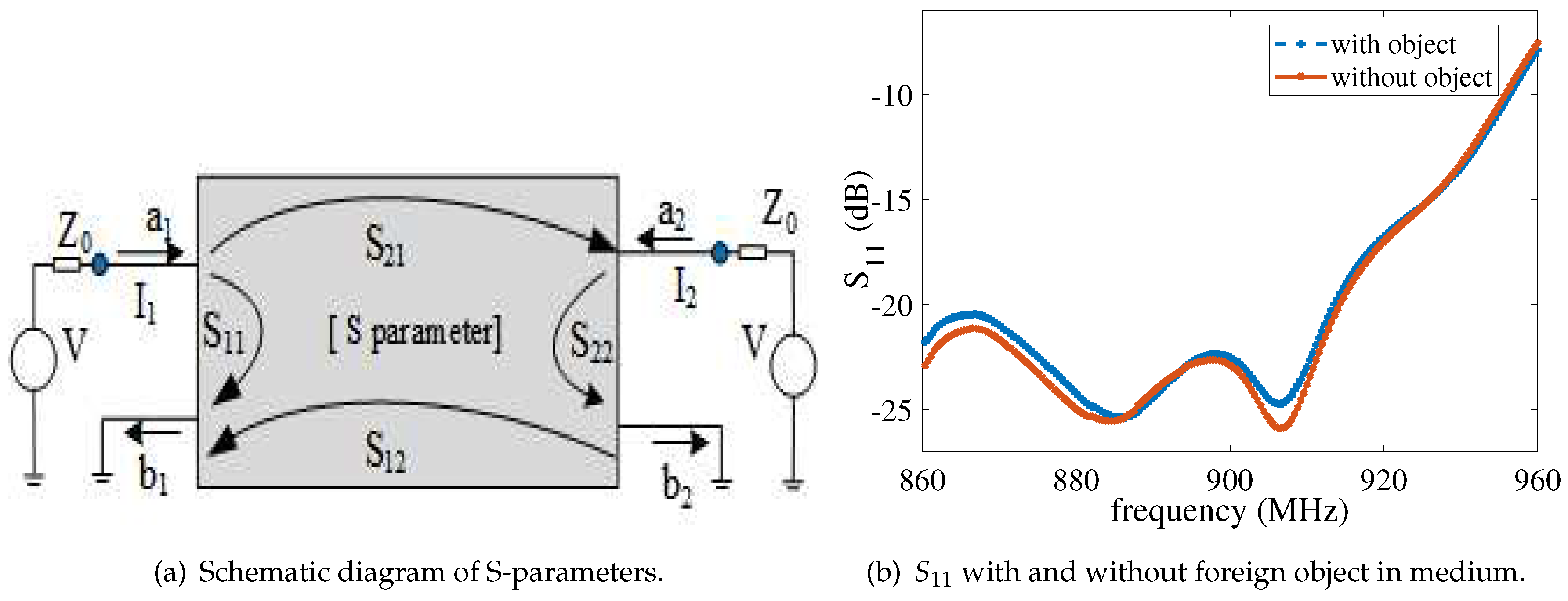
represents scattering parameters in a system, it is an important parameter in microwave transmission,
is also known as reflection coefficient, which describes the frequency domain characteristics of the transmission channel. Through the S-parameter, almost all the characteristics of the transmission channel can be known, as shown in
Figure 2a, it denotes the two ports network, where
denotes load impedance,
and
represent the incident and reflected signals from Port 1,
and
represent signals that of Port 2. We use Eq.
1 to represent the signals propagation in a circuit, where
and
represent
and
, respectively, and
and
represent the voltage and current of the corresponding ports. If
is used to represent the input reflection coefficient, i.e., input echo loss. Then we have the following expression
. In general, the S-parameter is a complex number. In this design, Eq.
2 is used to represent the value of
, where
denotes the amplitude of
, which is a real number.
For this system, single port (port 1) is utilized to perform the work of
as shown in
Figure 2a, the
can be read from a VNA device, we aim to sense the object by observing the changes of
using Eq.
2. According to the theory of electromagnetic wave transmission, signals will change if they are passing through two different media, thus, the signals will be scattered when the foreign objects are present in medium, some of the signals are reflected, some transmitted, and some are absorbed by the foreign object.
will be changed by the above reasons, indicating that it can be used to represent the presence of the object.
3.2. RSS based sensing model
Received Signal Strength (RSS) denotes the signal intensity when passing through a transmission line, in a clean wireless electromagnetic environment, the strength of the RFID received signal is obtained using the formula
, where
and
represent the power of the receiving and transmitting ports respectively, and
and
represent the antenna gain at the receiving and transmitting ports.
d denotes the distance between receiving and transmitting port. The above formula indicates that the RSS is only related to the distance
d if receiving and transmitting power is known. However, obtaining RSS through the above formula can be challenging. Typically, Eq.
3 is used to illustrate how RSS changes with
d [
32],
where
denotes the strength with distance
d from antenna to tag, in decibels.
denotes reference distance from a reference tag to antenna, it is a constant, so
is also a constant,
denotes the path loss factor,
denotes Gaussian noise with a mean of 0 and a variance
. To simplify the model, we use
RSS to show the RSS changes before and after there is/no foreign objects as illustrated in Eq.
4.
where d and d′ represent the paths of signal propagation in the medium before and after the objects are present. Assuming that the propagation path d′ is not changed after objects are present in medium, then we have
, there should be
. However, there is
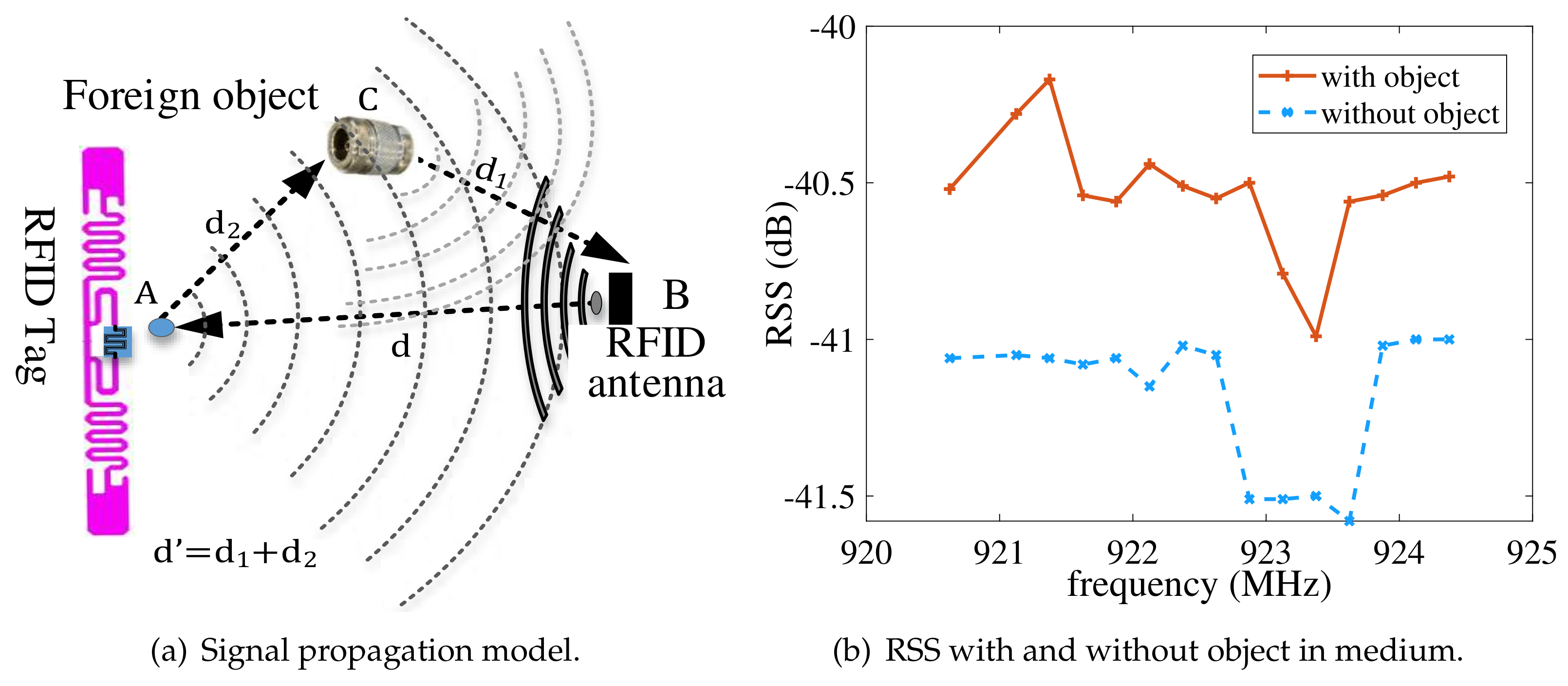
upon observation, indicating that the objects indeed change the signals paths. We plot
Figure 3b to illustrate RSS when there are objects in medium, indicating
can be a feature to sense foreign objects.
We provide a visual representation of the signal propagation path when a foreign object is present in the sensing space, as depicted in
Figure 3a. In the figure, points A, B, and C denote the tag, RFID antenna (responsible for receiving and transmitting), and the foreign object, respectively. When the electromagnetic wave from antenna B activates tag A, the tag responds by transmitting the signal back into the medium. In a uniform medium without object C, the signal path of the tag would be
with distance of
d. However, in the presence of object C, the transmission path can be mainly divided into two ways:
and
. The propagation paths of the signal is the superposition of the two paths, indicating that the object alters the signal’s trajectory. This alteration is in line with the triangle theorem, which states that the third side of a triangle is greater than the sum of the other two sides, i.e.
). Consequently, any changes in the signal path can lead to a corresponding change in
.
4. Design of sensing and localization algorithm
This section presents the design of the sensing and localization algorithm, consisting of two parts. Firstly, we investigate a method to determine the presence of foreign objects in the medium by observing changes in the tag signal when there are or are no objects. Secondly, leveraging the propagation characteristics of signals in the medium, we develop a mathematical model to determine the object’s position in a non-line-of-sight (NLOS) scene.
4.1. ’Euclidean distance ratio’ sensing algorithm
We have previously demonstrated the feasibility for sensing the object using RSS and
. In this section, we introduce the design of a foreign object sensing algorithm called the
algorithm, which relies on the Euclidean distance ratio. Assuming the Euclidean distance between two vectors
and
in space is defined as
, we utilize
to represent the feature vector of tag (i) collected by the system, and
d to represent the distance of signal propagation path,
=
and
=
represent the collected feature vectors of tag(i) when there is or is no object in the sensing medium. Then, the euclidean distance between
and
is expressed as Eq.
5,
Then, the sensing algorithm
is formulated as Eq.
6, where
represents Euclidean distance between vectors
and
for tag(i), Eq.
6 illustrates the euclidean distance ratio between the two feature vectors with and without foreign objects in medium. IF there is an object in the medium, the
will will changes according Eq.
6, because the object affects the propagation path of d’. In theory, when there is no foreign object near the tag, i.e. the signal path is not altered
, then
, otherwise
, which is referred to as abnormal
in tags. Thus,
can be used to sense the object near
, and its value vaguely indicates how far the object is from the tag. If there are multiple foreign objects in the sensing medium, their number can be determined by observing the abnormal
. However, in practical applications,
is usually greater than zero for there are noise in the Lab., and we address this issue by setting a threshold. If
from a tag exceeds the threshold, it is considered as an abnormal
that can be used to sense the foreign objects.
4.2. ’Projection’ localization algorithm
We have presented the sensing algorithm that can determine whether there are foreign objects or not in
Section 4.1. However, in practice, we urgently need to know their positions in order to remove them promptly. Therefor, in the following section, We introduce a method to locate the object based on
and RSS in NLOS scenes.
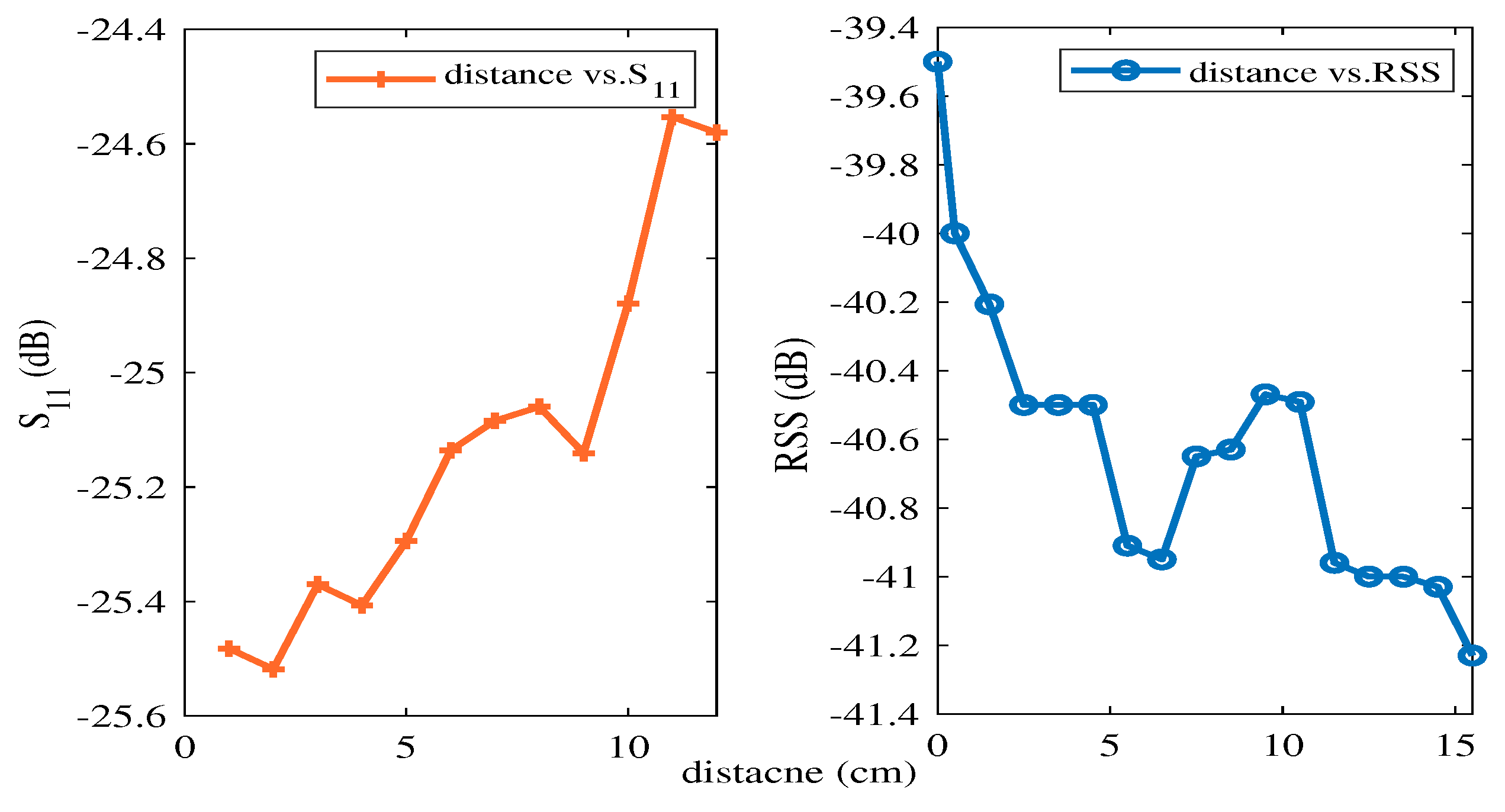
To verify the feasibility using
and RSS for localization,we conducted the following experiments to test the sensitivity of the above two features to position. We placed the foreign object C between the tag and the RFID antenna, moved its position, and observed the changes in
and RSS. As shown in
Figure 3a, C was gradually moved from A to B, and the impact of the position of C on
and RSS was observed separately (
can be read from an analog vector network analyzer, and RSS can be read from an RFID reader). The results showed that
and RSS vary with the foreign object position, indicating that the foreign object position is sensitive to both
and RSS, as illustrated in
Figure 4.
Based on the above observations, we conclude that
and RSS not only can sense the foreign objects, but also are sensitive to their positions. To obtain the 3-D position of foreign objects more accurately, we divided the sensing space into grids, as shown in
Figure 5a. We deployed
and
RFID tags on the planes XOY and XOZ respectively (represented by black hollow dots). These tags intersect with each other in the vertical direction of their respective planes, forming virtual intersection points (represented by blue solid dots). We use P(X, Y, Z) to represent the 3-D position virtual coordinates, while
and
represent the coordinates of RFID tags on the plane XOY and XOZ, respectively. If the point ’O’ is set as the coordinate of P(1,1,1), then the other points in the sensing space can be determined.
There are two steps to locate the object’s position, first, the system projects the objects onto the tag positions in plane XOY and plane XOZ respectively, then the intersection of the tags from the two planes is taken as object’s position in 3-D coordinate. Eq.
7 is used to obtain the tag projection position through the largest
, where tag(i) denotes the object’s projected position with tag number (i) whose
is the most abnormal.
denotes the possibility that object is projected on tag(i),
. It is reasonable to use probability to represent the projection position, as this system cannot accurately project foreign objects onto the tags but only in their vicinity. In fact, a object’s 3-D position is also a probability that is nearest to the grid, because the system uses the
from two planes to determine the position of the object in 3-D. So, this method may fail to locate the object. For example, the system obtains the positions
and
, and there is
, then no virtual intersection can be found, the localization fails.
To improve the success rate of localization, we propose a "sub-optimal" method to address the above issues. When the initial localization fails, the system selects the tag(k) and tag(l) with the second maximum from plane XOY and XOZ, respectively, the corresponding plane positions are and , if the system successes in localization, it will stop and return to position or , otherwise, if the localization is unsuccessful, the system persists in selecting the third maximum until successful localization is achieved.
4.3. BP neural network based object recognition
The Back-propagation (BP) network is the most widely applied model, it is a multi-layer feed-forward network trained using the error back-propagation algorithm, comprising input, hidden, and output layers. In comparison to deep learning networks with complex structures, BP network tends to perform more reliably on smaller datasets due to their relatively simple structure, which makes them less prone to overfitting. Here, we utilized RSS and as feature datasets to ’learn’ and ’train’ the network using a provided batch of corresponding input-output data to establish a specific network model. It identifies the signal features of various foreign objects, thereby achieving the desired outcome. The establishment of network models currently lacks a unified and comprehensive theoretical method and is generally determined by experience. In fact, the determination of parameters such as the input layer, hidden layer, and output layer constitutes the process of building the BP network model.
Input layer: The number of neurons in the input layer of the network is consistent with the tag feature parameters, which means that each feature value corresponds to a neuron in the input layer. This paper takes RSS and as feature parameters, therefore, the input layer contains two input neurons.
Hidden Layer: The number of neurons and layers in the hidden layer is generally determined based on the size of the data and personal experience. After repeated experiments, we set the optimal configuration for this layer as a single hidden layer with 25 neurons.
Output layer: This layer is determined by the output target of the network, which is determined by the number of foreign objects to be identified. There are four types of targets to be identified: metal, rock, rubber, and clod. Therefore, the number of neurons in this layer is set as 4.
After determining factors such as the number of layers, neurons in each layer, initial weight coefficients, transfer functions, learning algorithms, etc., a BP network is thereby established. Training a neural network system with ’expert knowledge’ is achieved only through continuous modification of network parameters. The network model is illustrated in
Figure 6, where
and
denote the weight of BP network. The excitation function is set as ’sigmod’, transfer function as ’tansig’, gradient descent BP training function as ’traingd’, network learning function as ’learngdm’, mean square error performance analysis function as ’mse’. The BP network model is integrated and encapsulated in the Matlab 6.5 toolbox, making it convenient to use for modeling.
5. Experiment and analysis
5.1. Experimental setup
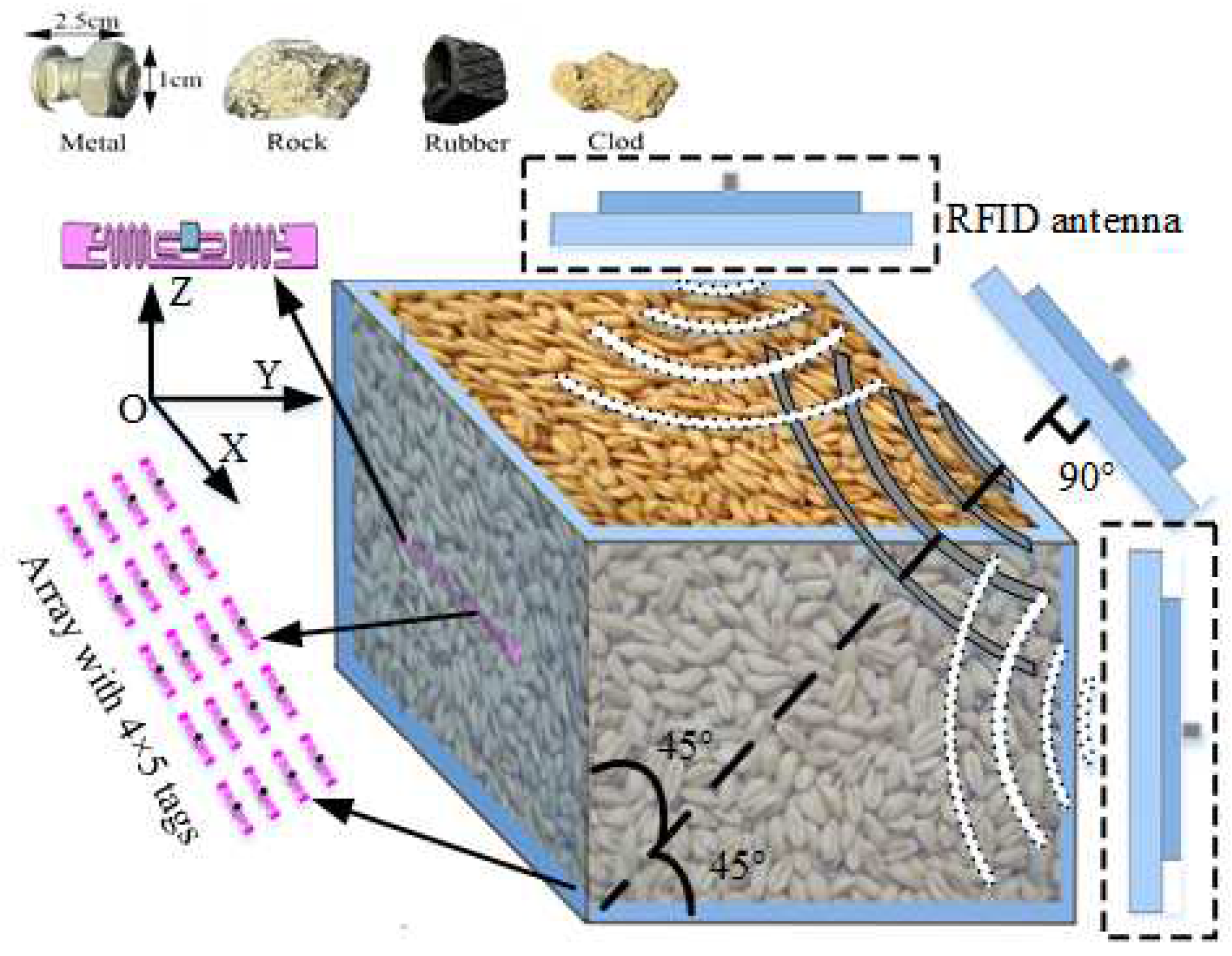
The experiment is performed in the sensing space with a size of 945mm× 520mm× 510mm. Seedless cotton and wheat are used as transmission medium to observe the properties of signal propagation in different media, Metal screws, rock, rubber block, and clod are taken as foreign objects for sensing target, as shown in
Figure 7. Alien 9640 with Higgs 3 chip is chosen as a tag, Laird2 S9028 polarized antenna as an RFID antenna, Impinj Speedway R220 as an RFID reader, and tektronix TTR506A as an analog Vector Network Analyzer. The system operates on a desktop computer with windows 10 OS. The RSS is read from Speedway R220 device, and
is read from Tektronix TTR506A.
Two tag matrices are deployed in the sensing medium, with one placed at the bottom (XOY plane) and the other on the side (XOZ plane). These tag matrices are designed to mitigate the coupling effect between the tags, following the recommendations mentioned in reference [
33]. According to the reference, it keeps a horizontal spacing of 22 cm and a vertical spacing of 17 cm between the tags. Consequently, two tag matrices are set up, with each comprised of a 5×4 matrix of tags, placed at the bottom (XOY plane) and on the side (XOZ plane), respectively, as shown in
Figure 7. To facilitate the data collection, one S9028 RFID antenna is placed above the XOY and XOZ planes, with 45-degree angle to the two planes (illustrated without dash box in
Figure 7) to enable effective communication with each tag from the two matrices on both planes, the RFID antenna move along the X axis of the container, collecting the feature vectors
each 50mm, where k=1,2 ⋯ 19. For a container with a length of 945mm, a total of 19 sets of feature vectors are recorded. In the deployment of this system,
represents the overall reflection coefficient in the tag matrix because the VNA cannot read
for a single tag. However, during the movement the antenna, the tag closest to the antenna tends to contribute the most to the reflection measured by
. This information proves valuable as it helps accurately associate the sensed objects with their corresponding tag positions. On the other hand, RFID reader has the capability to individually read
from each tag. This allows the RSS to provide signal indicators for a single tag, further enhancing the overall performance and functionality of the system.
We set the coordinates as illustrated in
Figure 5a, the 3-D coordinate is represented as P(X, Y, Z), with origin coordinate point ’O’ as the first point. If ’O’ is set as P(1,1,1), the positive direction of the X-axis should be P(2, 1, 1), P(3, 1, 1), P(4, 1, 1), P(5, 1, 1), respectively. Similarly, the positive direction of the Z-axis should be P(1, 1, 2), P(1, 1, 3), P(1, 1, 4), respectively. Therefore, there are 5×4×4 virtual point coordinates in space illustrated in
Figure 5.
5.2. Foreign object sensing
In this section, we validate the performance of the sensing algorithm when there are one or more foreign objects in the sensing space with media of seedless cotton and wheat, respectively.
Foreign objects are placed in the sensing space (filled with cotton or wheat), and the
values of each tag are obtained using the proposed algorithm, the
are plotted for each tag, as shown in
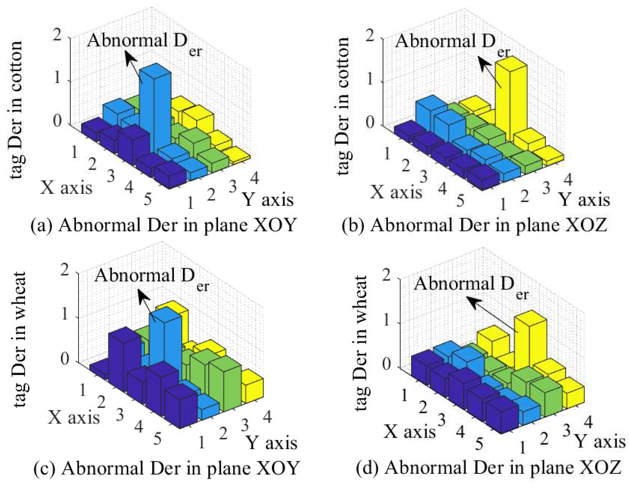
Figure 8, it presents the
when there is one object appears in medium, the indices of the X-axis, Y-axis represent the number of the tags, and Z-axis represent tag
respectively.
Figure 8a,b represent tag
in cotton,
Figure 8c,d represent tag
in wheat.
Figure 8 illustrated that the abnormal tag
can be an indicator to sense the target both in cotton and wheat, and the object in cotton is more easier sensed than that of in wheat because there are more noise
in wheat than in cotton. In addition, the properties of the media are also the factors impact the
algorithm performance.
However, in practice, there may be more objects in sensing space. So, in the following, we present the performance of the sensing algorithm when there are more objects.
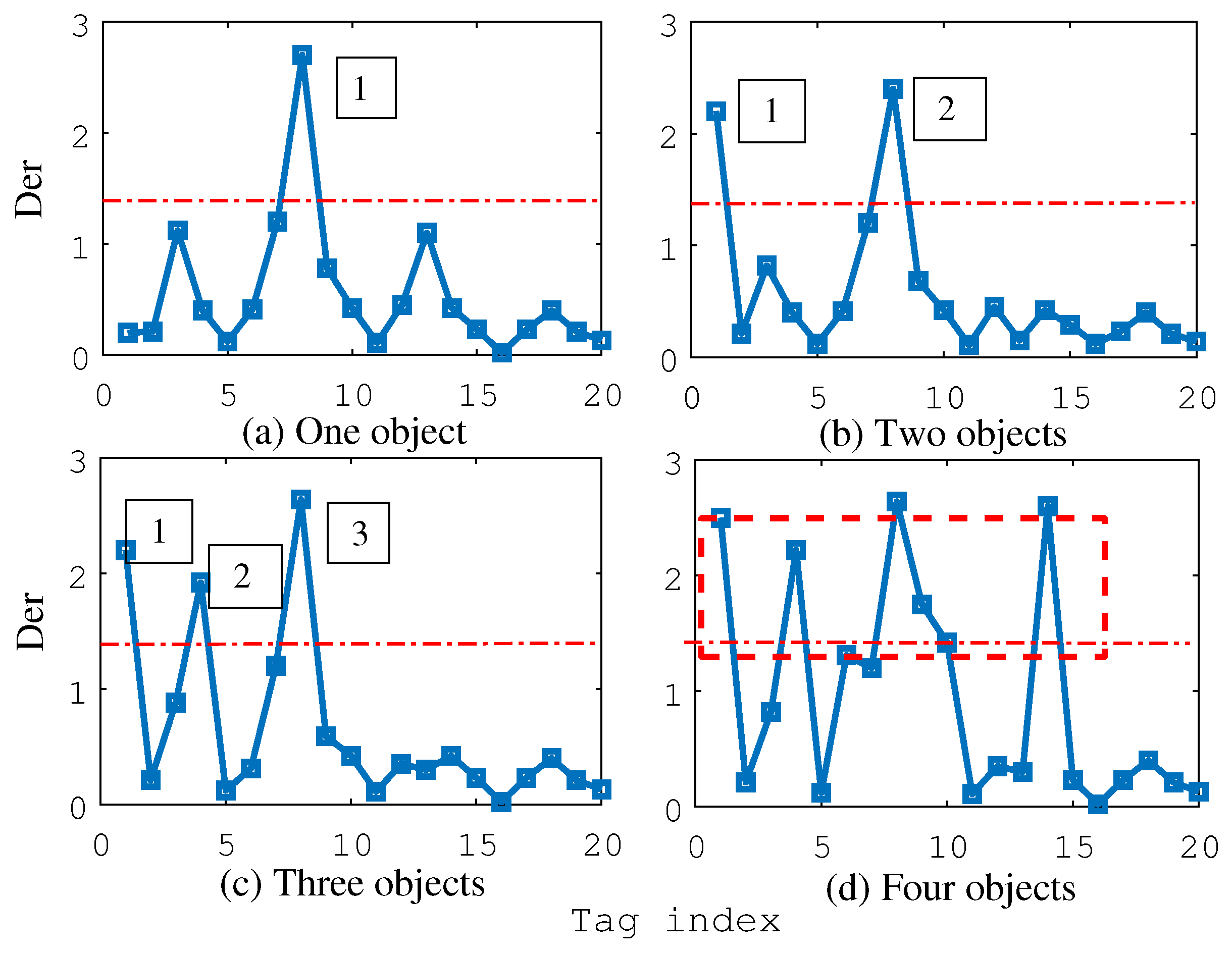
Figure 9 is plotted to show the abnormal
.
Figure 9a–d represent tag
corresponding to object of {rubber block}, {rubber block, rock}, {rubber block, rock, clod} and {rubber block, rock, clod, metal screw}, where red dashed line denotes the threshold for sensing objects (
>1.4).
is considered as abnormal if it is greater than 1.4.
The system can accurately determine the number of objects by counting the number of the abnormal tag
, as shown in
Figure 9a–c. However, it fails to count the correct number when there are more than four objects in the sensing space, as shown in
Figure 9d. The reason for this limitation is that the deployed tag matrix is too small to distinguish such a large number of targets. To address this issue, it is possible to consider increasing the size of the tag matrix, which would enhance the system’s ability to sense more targets. Furthermore, when metal foreign objects are present in medium, there are many abnormal
due to the strong shielding effect on electromagnetic signal. Therefore, for single object sensing, we predict that the system performs better when one metal object appears both in cotton and wheat medium because metal object has great impact on the signal. We will validate the idea in the following section by the projection localization algorithm.
5.3. Foreign object localization
In this section, we present the performance of the proposed localization algorithm through two steps: projecting the targets onto planes and achieving the virtual intersection (coordinate) in 3D space.
5.3.1. Projecting objects onto planes
Eq.
7 illustrated that the object’s position on planes can be represented using probability issue. Taking plane XOY as an example, in a matrix with
tags, each tag is assigned the probability of
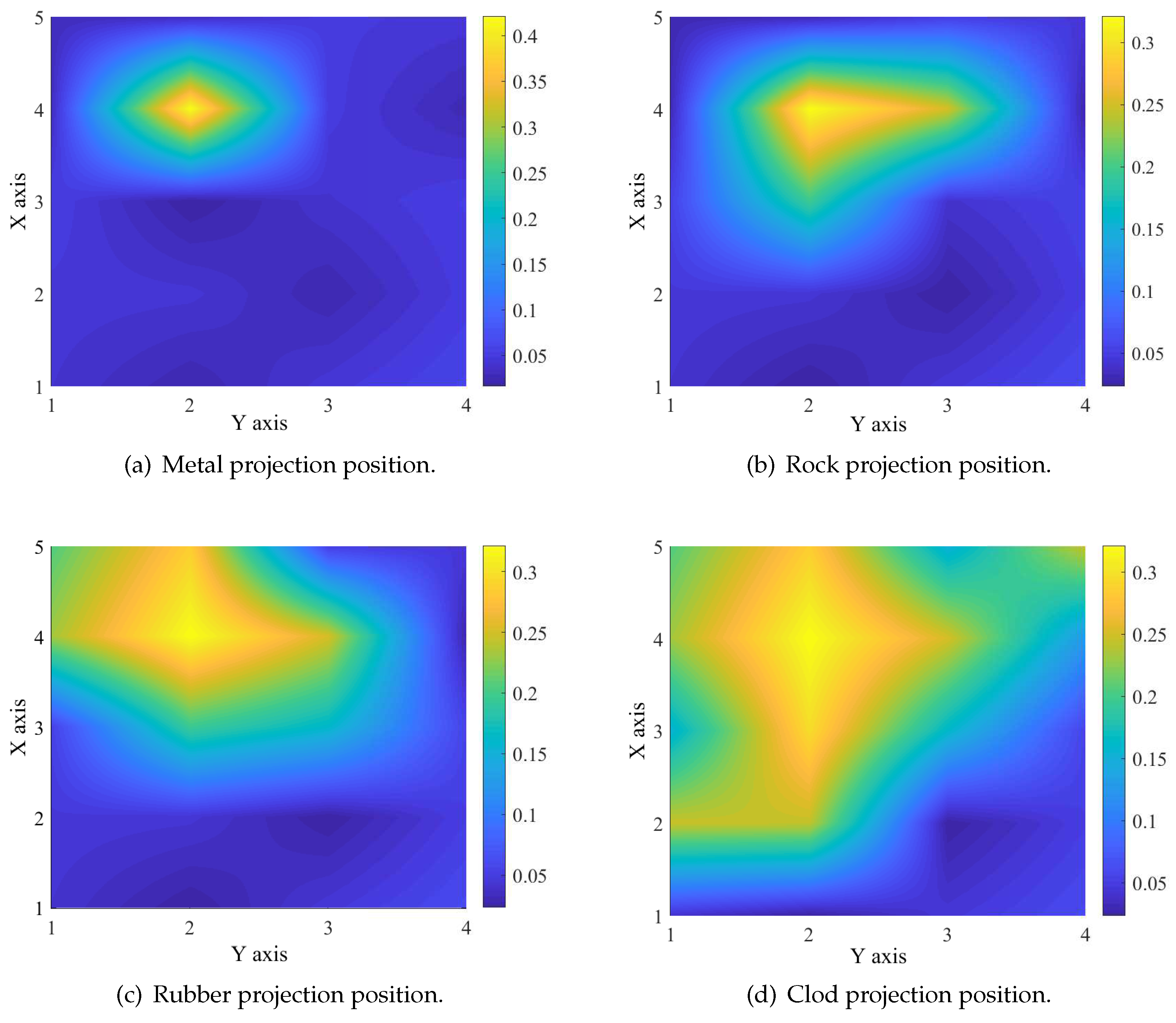
, a linear interpolation method is used to interpolate the matrix to creat a heat map that visualizes the possible projecting positions on the XOY plane, as shown in
Figure 10 and
Figure 11. These figures show the object projected onto the XOY plane in cotton and wheat medium, respectively. For metal and rock object, the figures show an accurate position both in cotton and wheat, as shown in
Figure 10a,b and
Figure 11a,b with position of
. For rubber block,
Figure 10c shows an accurate position in cotton medium, while, it achieves the exact projection position difficultly in wheat medium, as shown in
Figure 11c. For clod in wheat, We cannot achieve its projecting position at all, as shown in
Figure 11d.
From these observations, we can conclude that the accuracy of projecting varies depending on the properties of the objects. Metal objects can be accurately projected onto a plane, while the projection position of the clod is relatively blurry in wheat.
Figure 10 and
Figure 11 also depict the influence of the medium on the system. The projection accuracy is better in cotton medium than in wheat medium, which can be attributed to the dielectric properties of cotton and wheat. Cotton, being a non-magnetic substance without moisture content, allows for easier penetration of electromagnetic waves compared to wheat, which is a weakly magnetic substance due to its moisture content.
5.3.2. Locating objects in 3D space
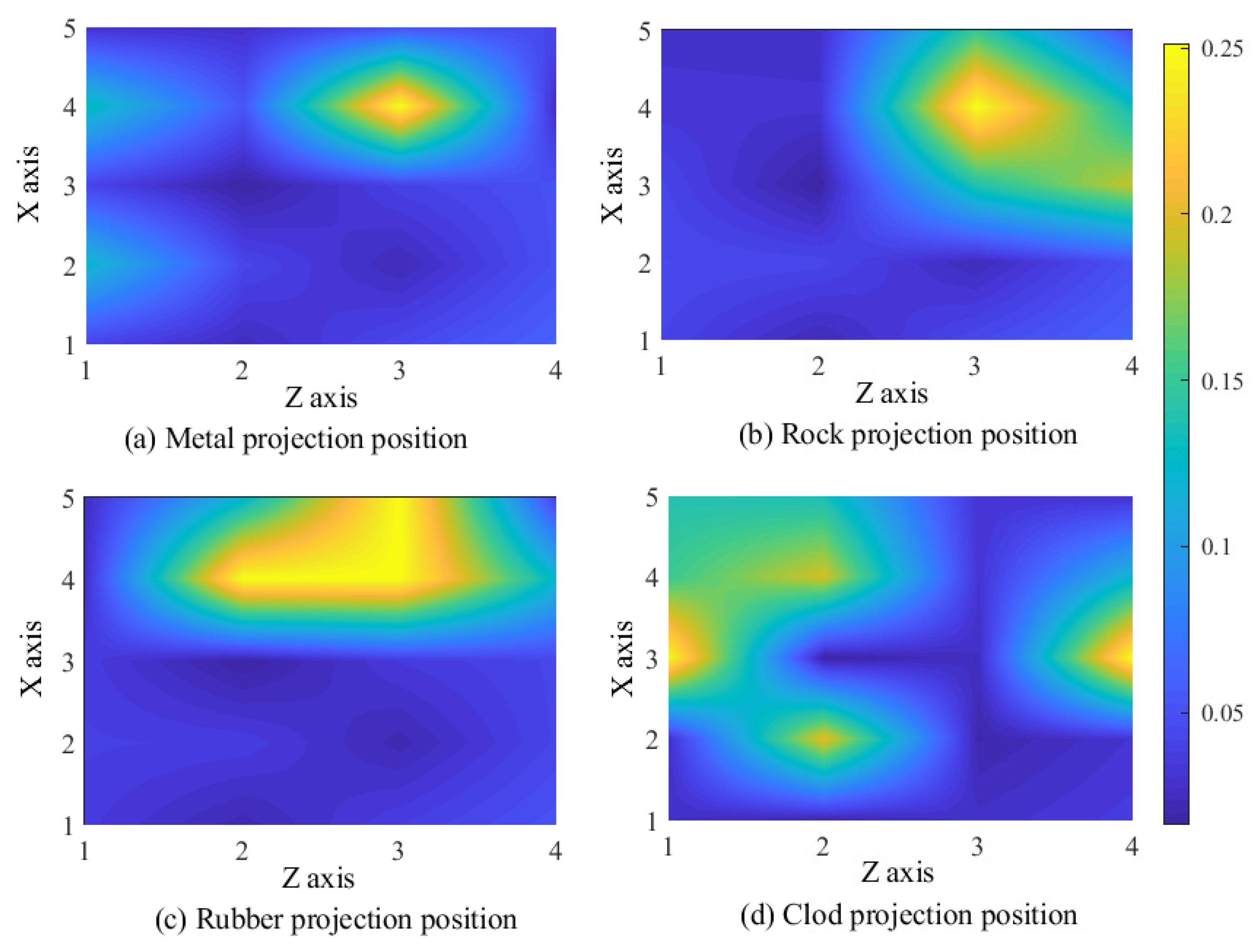
To locate the object in 3D space, we need to obtain the projection position both on XOY and XOZ plane. So, we plot the projection position in plane XOZ as shown in
Figure 12a–d, which represent the possible position of metal, rock, rubber and clod in wheat, respectively. By observing the figures, we obtained the projection positions of the object on two planes and recorded these positions in
Table 1. According to the localization algorithm, when
, the localization is considered successful.
Table 1 illustrated that metal and stone can be easily located, while rubber block have two possible positions (one of which is the incorrect position of
, whereas clod fail to be located. This once again indicates the conclusion that clod is difficult to be located.
For comparison, we take non-magnetic cotton as an example and use the same method to test the localization performance of foreign objects in cotton. The results are shown in
Table 2. The metal, rubber and rock blocks were also accurately located, however the clod was positioned with two possible locations, one of which is correct. This indicates that clod failed to be located in wheat, but succeeded in cotton. This verifies that object localization algorithm is not only related to the properties of the objects themselves, but also to the media where the objects are placed.
To quantify the positioning performance of the algorithm, we employed a statistical approach to determine the system’s localization accuracy. We randomly placed the objects in the sensing space, obtained the positions of these objects using the projection localization algorithm, repeated this process 88 times, and compared the results with the actual positions. The successful localization rate is presented in
Table 3, it indicates that the initial localization accuracy of metals is highest both in wheat and cotton, however, the localization rate of clod is only 55.6%, which is not satisfactory. Overall, the localization accuracy in cotton is higher than that in wheat, which once again validates the conclusion that electromagnetic wave signals perform better in non-magnetic media than in magnetic or weak magnetic media.
In
Table 1 and
Table 2, there are the cases that algorithm fails in localization for clod. For example, while clod in wheat was not successfully located, clod in cotton was located at two different positions. This affects the reliability of the system. To address this issue, we are considering two methods to enhance the system’s performance. The first approach involves implementing the "sub-optimal solution" method mentioned in previous sections, i.e., if the initial localization failure, the system searching for the second potential location of the object until successful localization is achieved. The second approach is to add one more RFID antenna and adjust the positions of the two antennas (as shown in
Figure 7, the RFID antennas with black dashed box). This adjustment is made to align them directly with two tag matrices (in XOY plane and XOZ plane), ensuring that the electromagnetic wave propagation direction is perpendicular to the tag matrices. This aims to improve the overall reliability and accuracy of the system.
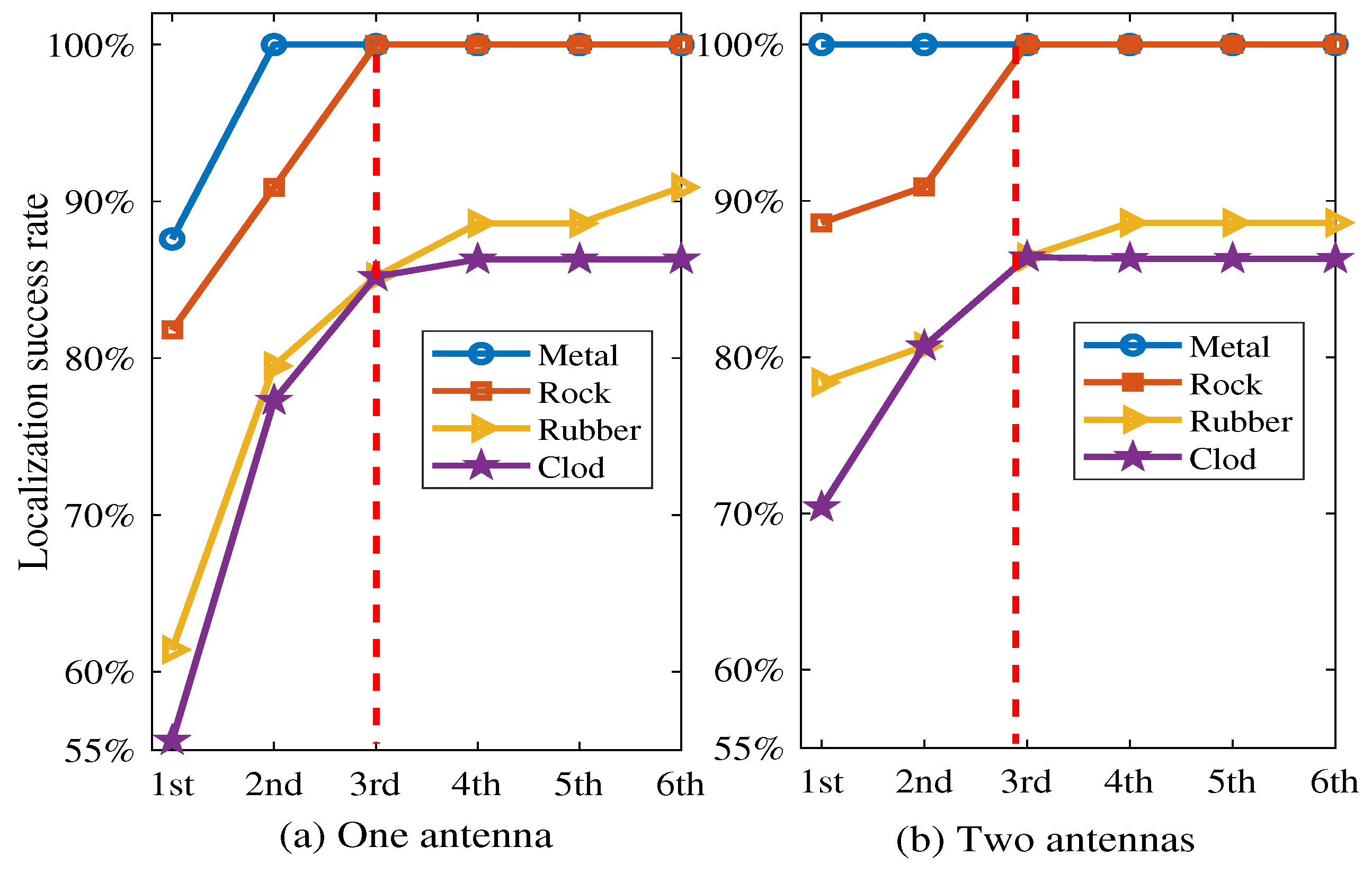
Figure 13a shows the success rate of object localization after applying the Sub-optimal algorithm using only one RFID antenna. The vertical axis in the figure represents the success rate of localization, the horizontal axis represents the number of re-locations, where ’1st’ represents the success rate for the initial localization. The localization success rate of metals and stones reached 100% after the second and the third re-location, the rubber and clod improved from 55.6% and 61.4% to around 85% after three re-locations. However, the accuracy improvement of rubber and clod is not significant after three more re-locations. This indicates that the system performance has reached its upper limit.
To further improve the system performance, we adjusted the deployment of RFID antennas, as illustrated in
Figure 7. The two dashed boxes represent the deployment positions of the two RFID antennas. They are oriented towards the tag matrices separately, collecting the corresponding tag features for each. The original intention of this deployment is to facilitate the projection of foreign objects near the correct tags, with the expectation of improving projection accuracy, the result is plotted in
Figure 13b shows the variation in localization success rate as the number of re-locations increases when two RFID antennas are deployed in the sensing space. Compared with
Figure 13a, it can be seen that the first localization success rate has been significantly improved when using dual RFID antennas. However, after using sub-optimal algorithms to improve system performance, it was found that the overall localization success rate of the system did not significantly improve. Although the design of dual antennas increases system costs, it fails to bring significant improvements to system performance. On the contrary, although a single antenna has a lower success rate in initial localization, the sub-optimal algorithm can compensate for this deficiency and also reduce system costs. Therefore, the single antenna combined with Sub-optimal algorithm can work well to show a satisfactory performance.
5.4. Objects recognition
BP neural network is a tool packaged in Matlab 6.5, which is very convenient. Based on the parameters set by developers, a network model can be established through data training. we represent the output target of the network model in the form of a vector. As there are four types of objects to be recognized, we set the output targets as , they represent the output targets for metal, rock, rubber, and clod,respectively. The closer the output vector is to the target vector T, the greater the similarity.
In experiment, we selected tags from two planes as the collection targets. There are
tags in each plane, and 2 features sensed from each tag. For one RFID antenna method, it needs to move 19 steps to scan the entire sensing space (2 planes of XOY and XOZ), resulting in a data volume of
being collected. Furthermore, to make the BP model more robust, the experimental data from cotton and wheat (2 media) were mixed together, resulting in
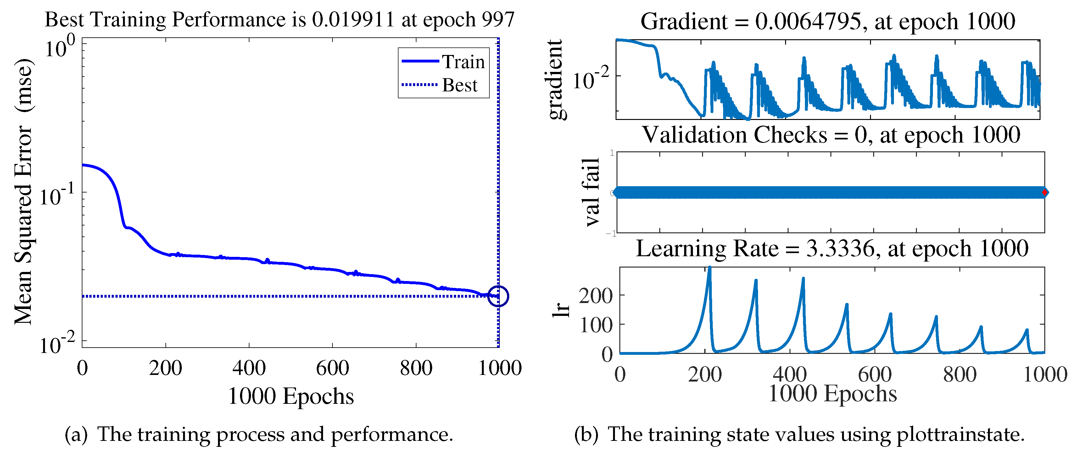
=3040 samples. Therefore, for such a small-scale samples, the BP neural network model is fully capable with better efficiency. We set the maximum training steps to 2000, with a training minimum error of 0.001. The learning rate was set to 0.005. The training process and results are illustrated in
Figure 14 and
Table 4.
We placed the four types of objects in the media, collected data, and fed them into the model, the output vectors is illustrated in the
Table 4, from left to right, they represent rock, metal, clod, and rubber. It can be observed that for the output target vectors of rock (
) and metal (
), their corresponding elements are very close to 1 (0.99959, 0.999691), while the other elements are close to 0, indicating that the model can recognize these two types of objects well. The output vectors of the clod (
) and the rubber (
) correspond to elements 0.97990 and 0.910530, respectively. However, the highest values for other elements are 0.634173 and 0.303177. This implies a slight weaker capability of the BP model in identifying clod and rubber.
6. Conclusions
We introduced a method for wireless object localization and recognition under NLOS, investigated the propagation patterns of RFID signals in weak magnetic and non-magnetic media, revealing the principle of foreign object recognition and localization based on tag feature signals. Unlike traditional sensing methods based on RFID, this method does not require attaching tags to the target, we achieved non-contact sensing, recognition and localization through a tag matrix. The research results indicate that using a single RFID antenna combined with Sub-optimal algorithm can successfully sense, locate and recognize four common objects in wheat and cotton.
The study has a wide range of practical applications and can be directly applied in other fields, such as airport security, liquid foreign material detection, etc. However, it is still in preliminary, and there are still some limitations. For instance, this paper did not conduct research on the sensing depth in media, resulting in the inability to sense the maximum measurement range. Furthermore, a more extensive range of media should be examined. The current presentation of system performance is limited to two media (cotton and wheat), which may not be sufficiently representative. Testing the system’s robustness would require the inclusion of a broader range of media in future studies.
Author Contributions
Conceptualization, E.S. and W.Y.; methodology, W.Y. and S.D.; validation, E.S., S.G.; investigation, E.S., S.G.; resources, W.Y.; data curation, E.S., S.G.; writing—original draft preparation, E.S. and S.G.; writing—review and editing, E.S.; visualization, E.S.; supervision, W.Y.; project administration, E.S. and W.Y.; funding acquisition, E.S. and W.Y. All authors have read and agreed to the published version of the manuscript.
Funding
This research was funded by the National Science Foundation of Henan (No.222300420004) and Major Public Welfare Special Projects of Henan Province (No.201300210100), NSFC (No. 62172141, 61772173, 61741107), and Key scientific Research Projects of Colleges and Universities in Henan Province in 2022 (22B520021).
Institutional Review Board Statement
Not applicable.
Informed Consent Statement
Not applicable.
Data Availability Statement
The data presented in this study are available in
Table 1,
Table 2 and
Table 3, and
Figure 14. The other data are available upon request from the corresponding author.
Conflicts of Interest
The authors declare no conflict of interest.
References
- Yang, C.; Wang, X.; Mao, S. RFID tag localization with a sparse tag array. IEEE Internet of Things Journal 2022, 9, 16976–16989. [Google Scholar] [CrossRef]
- Gomes, E.L.; Fonseca, M.; Lazzaretti, A.E.; Munaretto, A.; Guerber, C. Clustering and Hierarchical Classification for High-Precision RFID Indoor Location Systems. IEEE Sensors Journal 2022, 22, 5141–5149. [Google Scholar] [CrossRef]
- Zhang, J.; Lyu, Y.; Patton, J.; Periaswamy, S.C.G.; Roppel, T. BFVP: A Probabilistic UHF RFID Tag Localization Algorithm Using Bayesian Filter and a Variable Power RFID Model. IEEE Transactions on Industrial Electronics 2018, 65, 8250–8259. [Google Scholar] [CrossRef]
- Mahajan, P. Internet of things revolutionizing Agriculture to Smart Agriculture. In Proceedings of the 2021 2nd Global Conference for Advancement in Technology (GCAT), Bangalore, India, 2021; pp. 1–6. [Google Scholar]
- Liang, B.; Liu, X.; Wan, Y.; Cheng, S.; Liu, J.; Xu, C. Poster: Empower Smart Agriculture with RFID Reference Infrastructure. In Proceedings of the 2023 20th Annual IEEE International Conference on Sensing, Communication, and Networking (SECON), Madrid, Spain, 2023; pp. 72–73. [Google Scholar]
- Bothe, A.; Bauer, J.; Aschenbruck, N. RFID-assisted Continuous User Authentication for IoT-based Smart Farming. In Proceedings of the 2019 IEEE International Conference on RFID Technology and Applications (RFID-TA), Pisa, Italy, 2019; pp. 505–510. [Google Scholar]
- Pezzuolo, A.; Guo, H.; Guercini, S.; Marinello, F. Non-contact feed weight estimation by RFID technology in cow-feed alley. In Proceedings of the 2020 IEEE International Workshop on Metrology for Agriculture and Forestry (MetroAgriFor), Trento, Italy, 2020; pp. 170–174. [Google Scholar]
- Manzari, S.; Occhiuzzi, C.; Nawale, S.; Catini, A.; Di Natale, C.; Marrocco, G. Humidity Sensing by Polymer-Loaded UHF RFID Antennas. IEEE Sensors Journal 2012, 12, 2851–2858. [Google Scholar] [CrossRef]
- F. Bernardini et al. RFID-Based Tracking for Worker Safety in Industrial Scenario. 2021 IEEE International Conference on RFID Technology and Applications (RFID-TA), Delhi, India, 2021, pp. 44-47.
- Raptopoulos, A.; Yioultsis, T.; Dimitriou, A.G. Particle Filter Object Tracking by a Handheld UHF RFID Reader. In Proceedings of the 2019 IEEE International Conference on RFID Technology and Applications (RFID-TA), Pisa, Italy, 2019; pp. 342–347. [Google Scholar]
- Yang, C.; Wang, Z.; Mao, S. RFPose-GAN: Data Augmentation for RFID based 3D Human Pose Tracking. In Proceedings of the 2022 IEEE 12th International Conference on RFID Technology and Applications (RFID-TA), Cagliari, Italy, 2022; pp. 138–141. [Google Scholar]
- Yang, C.; Tao, Y.; Man, H.; Zhu, W. Dielectric Sensing-aid Structure for RFID Tag. In Proceedings of the 2019 IEEE International Conference on RFID Technology and Applications (RFID-TA), Pisa, Italy, 2019; pp. 248–251. [Google Scholar]
- Kumar, D.; Muhammad, N. A Survey on Localization for Autonomous Vehicles. IEEE Access 2023, 11, 115865–115883. [Google Scholar] [CrossRef]
- Feng, J.; Wang, L.; Li, J.; Xu, Y.; Bi, S.; Shen, T. Novel LiDAR-assisted UWB positioning compensation for indoor robot localization. In Proceedings of the 2021 International Conference on Advanced Mechatronic Systems (ICAMechS), Tokyo, Japan, 2021; pp. 215–219. [Google Scholar]
- Haider, U.A.; Noman, M.; Ullah, H.; Tahir, F.A. A Compact Chip-less RFID Tag for IoT Applications. In Proceedings of the 2020 IEEE International Symposium on Antennas and Propagation and North American Radio Science Meeting, Montreal, QC, Canada, 2020; pp. 1449–1450. [Google Scholar]
- Ni, L.M.; Liu, Y.; Lau, Y.C.; Patil, A.P. LANDMARC:indoor location sensing using active RFID. In Proceedings of the First IEEE International Conference on Pervasive Computing and Communications, 2003. (PerCom 2003), Fort Worth, TX, USA, 2003; pp. 407–415. [Google Scholar]
- Yuri Álvarez López; María Elena de Cos Gómez; Fernando Las-Heras Andrés. A received signal strength RFID-based indoor location system. Sensors and Actuators A: Physical 2017,3, 118-133. [CrossRef]
- Fu, Y.; Wang, C.; Liu, R.; Liang, G.; Zhang, H.; Ur Rehman, S. Moving Object Localization Based on UHF RFID Phase and Laser Clustering. Sensors 2018, 18, 825. [Google Scholar] [CrossRef] [PubMed]
- Ur Rehman, S.; Liu, R.; Zhang, H.; Liang, G.; Fu, Y.; Qayoom, A. Localization of Moving Objects Based on RFID Tag Array and Laser Ranging Information. Electronics 2019, 8, 887. [Google Scholar] [CrossRef]
- Shaonan Chen; Heng Ning; Lin Guo; Feng Sun; Yufeng Xiao; Ran Liu. Tracking multiple dynamic objects by a combination of laser ranging and UHF RFID phase information. Journal of Physics: Conference Series 2023, 2595, 012007. [CrossRef]
- Eric Rigall; Xianglong Wang;Shu Zhang, et al. A fast and accurate rfid tag positioning method based on AoA hologram and hashtables. Computer Communications. 2023, 202, 135-144. [CrossRef]
- Qiu, L.X.; Huang, Z.Q.; Da, L.I. 3d tag location aware scheme based on phase interferometric for rfid applications. Chinese Journal of Computers 2019, 11, 2512–2525. [Google Scholar]
- Chuyu Wang; Jian Liu; Yingying Chen; et al. Rf-kinect: A wearable RFID-Based approach towards 3d body movement tracking. Proc. ACM Interact. Mob. Wearable Ubiquitous Technol 2018,2,28-41. [CrossRef]
- Arboleya, A.; Laviada, J.; Álvarez-López, Y.; Las-Heras, F. Real-Time Tracking System Based on RFID to Prevent Worker–Vehicle Accidents. IEEE Antennas and Wireless Propagation Letters 2021, 20, 1794–1798. [Google Scholar] [CrossRef]
- Gui, L.; Xu, S.; Xiao, F.; Shu, F.; Yu, S. Non-Line-of-Sight Localization of Passive UHF RFID Tags in Smart Storage Systems. IEEE Transactions on Mobile Computing 2022, 21, 3731–3743. [Google Scholar] [CrossRef]
- Ma, H.; Wang, K. Fusion of RSS and Phase Shift Using the Kalman Filter for RFID Tracking. IEEE Sensors Journal 2017, 17, 3551–3558. [Google Scholar] [CrossRef]
- Wen, K.; Seow, C.K.; Tan, S.Y. An Indoor Localization and Tracking System Using Successive Weighted RSS Projection. IEEE Antennas and Wireless Propagation Letters 2020, 19, 1620–1624. [Google Scholar] [CrossRef]
- Ma, Y.; Liu, H.; Zhang, Y.; Jiang, Y. The Influence of the Nonideal Phase Offset on SAR-Based Localization in Passive UHF RFID. IEEE Transactions on Antennas and Propagation 2020, 68, 6346–6354. [Google Scholar] [CrossRef]
- Chen, K.; Ma, Y.; Liu, H.; Liang, X.; Fu, Y. Trajectory-Robust RFID Relative Localization Based on Phase Profile Correlation. IEEE Transactions on Instrumentation and Measurement 2023, 72, 1–13. [Google Scholar] [CrossRef]
- Xiong, H.; Shen, C.; Ye, T.T. Broadband and Fast Carrier Cancellation for Backscattered RFID Communications. IEEE Microwave and Wireless Components Letters 2021, 31, 84–87. [Google Scholar] [CrossRef]
- G. Wang et al. A Generalized Method to Combat Multipaths for RFID Sensing. IEEE/ACM Transactions on Networking 2023,31(1), 336-35. [CrossRef]
- Ghassemzadeh, S.S.; Greenstein, L.J.; Kavcic, A.; Sveinsson, T.; Tarokh, V. UWB indoor path loss model for residential and commercial buildings. In Proceedings of the 2003 IEEE 58th Vehicular Technology Conference. VTC 2003-Fall (IEEE Cat. No.03CH37484), Orlando, FL, USA, 2003; 5, pp. 3115–3119. [Google Scholar]
- H. Yigang; X. Peiliang; z. Lei et al. Study on frequency shift in mutual coupling effect of ultra-high-frequency radio frequency identification near-field system. Journal of Electronics and Information 2019, 41(3), 602-610. [CrossRef]
|
Disclaimer/Publisher’s Note: The statements, opinions and data contained in all publications are solely those of the individual author(s) and contributor(s) and not of MDPI and/or the editor(s). MDPI and/or the editor(s) disclaim responsibility for any injury to people or property resulting from any ideas, methods, instructions or products referred to in the content. |
© 2023 by the authors. Licensee MDPI, Basel, Switzerland. This article is an open access article distributed under the terms and conditions of the Creative Commons Attribution (CC BY) license (https://creativecommons.org/licenses/by/4.0/).
